CLPNets: Coupled Lie-Poisson Neural Networks for Multi-Part Hamiltonian Systems with Symmetries
Abstract
To accurately compute data-based prediction of Hamiltonian systems, especially the long-term evolution of such systems, it is essential to utilize methods that preserve the structure of the equations over time. In this paper, we consider a case that is particularly challenging for data-based methods: systems with interacting parts that do not reduce to pure momentum evolution. Such systems are essential in scientific computations. For example, any discretization of a continuum elastic rod can be viewed as interacting elements that can move and rotate in space, with each discrete element moving on the configuration manifold, which can be viewed as the group of rotations and translations . For an isolated elastic rod, the system is invariant with respect to the same group of rotations and translations. For individual elastic elements, due to this symmetry, the equations can be written as Lie-Poisson equations for the momenta, which are vector variables. For several elastic elements, the evolution involves not only the momenta but also the relative positions and orientations of the particles. Although such a system can technically be written in a way similar to a Lie-Poisson system with a Poisson bracket, the presence of Lie group-valued elements, such as relative positions and orientations, poses a problem for applying previously derived methods for data-based computing.
In this paper, we develop a novel method of data-based computation and complete phase space learning of such systems. We follow the original framework of SympNets (Jin et al., 2020), building the neural network from phase space mappings that are canonical, and transformations that preserve the Lie-Poisson structure (LPNets) as in (Eldred et al., 2024). To find adequate neural networks for Poisson systems including relative orientations, we derive a novel system of mappings that are built into neural networks describing the evolution of such systems. We call such networks Coupled Lie-Poisson Neural Networks, or CLPNets. We consider increasingly complex examples for the applications of CLPNets, starting with the rotation of two rigid bodies about a common axis, progressing to the free rotation of two rigid bodies, and finally to the evolution of two connected and interacting components, describing the discretization of an elastic rod into two elements. Our method preserves all Casimir invariants of each system to machine precision, irrespective of the quality of the training data, and preserves energy to high accuracy. Our method also shows good resistance to the curse of dimensionality, requiring only a few thousand data points for all cases studied, with the effective dimension varying from three in the simplest cases to eighteen in the most complex. Additionally, the method is highly economical in memory requirements, requiring only about 200 parameters for the most complex case considered.
keywords:
Neural equations, Data-based modeling, Long-term evolution, Hamiltonian Systems, Poisson brackets[1]organization = Computer Science Research Institute, addressline=Sandia National Laboratory, 1450 Innovation Pkwy SE, city=Albuquerque, state = NM, postcode=87123, country=USA
[2]organization = Division of Mathematical Sciences, addressline=Nanyang Technological University, city=637371, country=Singapore
[3]organization=Department of Mathematical and Statistical Sciences, addressline=University of Alberta, city=Edmonton, postcode=T6G 2G1, state=Alberta, country=Canada
1 Introduction
1.1 Physical relevance and importance for applications
Many physical systems contain several interacting parts of a similar nature. Individual parts of these systems possess their own dynamics and simultaneously contribute to the combined dynamics of the system through their interaction with other parts. Perhaps the most apparent examples of such systems are provided by the discretization of continuum mechanics, for example, elastic rods in the Lagrangian setting. A discretization based on either finite elements or a lattice will lead to a finite number of interacting elastic elements. These elements have their own linear and angular momenta, and the elastic energy depends on the relative position and orientation of these elements, with interactions limited to the nearest neighbors. Thus, understanding how to solve the combined dynamics of coupled systems is essential for practical computations in continuum mechanics. Besides the discretization of continuum elastic systems, other examples include systems modeling macromolecular conformations, such as those described by (Banavar et al., 2007), which use finite-size elements. Applications of this type abound in robotics, especially in soft robots and manipulators (Chirikjian, 1994; Mengaldo et al., 2022). The goal of this paper is to develop data-based, structure-preserving computing methods for such systems. Other physical examples of these kinds of systems include the dynamics of tree-like structures (Amirouche, 1986; Ider and Amirouche, 1989), see also (Nieuwenhuis et al., 2018) for applications of tree-like structures to energy harvesting. Another application is the dynamics of polymers that may have nonlocal interactions through, for example, electrostatic charges (Ellis et al., 2010), and may have non-trivial dendronized topology in their structure (Gay-Balmaz et al., 2012).
In order to compute the evolution of these systems in a traditional way, one needs to assume an exact formula for the Hamiltonian of the system. In some cases, such a formula may be highly complex, involving many parameters and even having an unclear functional form. That ambiguity is especially pronounced in the elasticity arguments related to biological materials, as numerous suggestions for elastic energy have been proposed. This is evident, for instance, in the elastic energy components of brain tissue mechanics (Jiang et al., 2015; de Rooij and Kuhl, 2016; Mihai et al., 2017). In addition to the inherent complexity of elasticity, the dynamics of brain tissue are believed to include viscoelastic components (Calhoun et al., 2019). Thus, for cases where the exact form of mathematical models is unknown, it is advantageous to develop data-based modeling methods. These methods circumvent the complexity of constructing exact models for simulations and only require the general form of these mathematical models, such as the variables they may depend on or the symmetries they may obey.
We thus develop data-based numerical methods that fit into the framework of Physics-Informed Neural Networks (PINNs) for these systems. In this paper, we focus on developing computational methods applicable to Hamiltonian systems where friction can be neglected. As we describe below, traditional PINNs are difficult to apply directly to Hamiltonian systems, so we seek structure-preserving methods capable of accurately describing the systems’ long-term dynamics. We begin with a review of the current literature on data-based computation of Hamiltonian systems.
1.2 Relevant work related to data-based computing of Poisson systems
Purely data-based methods rooted on Machine Learning (ML) have been successful in interpreting large amounts of unstructured data. However, applying ML methods directly to big data for scientific and industrial purposes, without a deep understanding of the underlying engineering and physics, presents challenges. To tackle these issues, Physics Informed Neural Networks (PINNs) have been developed (Raissi et al., 2019). Given the breadth of PINNs literature, a comprehensive overview is beyond the scope here; interested readers are referred to recent reviews (Karniadakis et al., 2021; Cuomo et al., 2022; Kim and Lee, 2024) for references, literature reviews, and discussions on the advantages and disadvantages of these methods. In this approach, the system’s evolution over time is assumed to be described by a quantity belonging to some phase space, and the system’s motion is approximated by a governing equation:
| (1) |
Here, and can be either finite-dimensional, forming a system of ODEs, or infinite-dimensional, forming a system of PDEs where they depend, for example, on additional spatial variables and derivatives with respect to these variables. In the regular PINNs approach, the initial conditions, boundary conditions, and the ODEs themselves form part of the loss function. Subsequently, a neural network is designed to take the independent variable time (and perhaps the independent spatial variables ) and predict the unknown function representing the solution. Due to the structure of neural networks, for a known set of weights, the derivatives of the solution with respect to the independent variables, and thus the function representing the equation (1), , can be computed analytically at given points, as well as the value of the function at specified points (for example, initial conditions) and, if necessary, boundary conditions. For a given set of weights and activating functions in a neural network, the exact values of temporal (and, if necessary, spatial) derivatives are computed using the method of automatic differentiation (Baydin et al., 2018) to machine precision. Consequently, the loss can be computed as a function of the neural network’s weights and optimized during the learning procedure. PINNs offer computational efficiency, with reported speedups exceeding 10,000 times for evaluations of solutions in complex systems like weather (Bi et al., 2023; Pathak et al., 2022), accompanied by a drastic reduction of the energy consumption needed for computation. PINNs are thus highly valuable in practical applications and have been implemented as open-source software in Python and Julia. Readers can easily find numerous open-source packages for implementing PINNs on GitHub, developed as individual or group projects, as well as products from large industry efforts, such as Nvidia’s Modulus.
In spite of their successes, there are still many uncertainties in the applications of PINNs. For example, PINNs may struggle with systems that have dynamics with widely different time scales (Karniadakis et al., 2021), although numerous methods of solutions for this problem have been suggested Kim and Lee (2024). Challenges have been identified for PDEs featuring strong advection terms (Krishnapriyan et al., 2021). Systems with very little friction, such as Hamiltonian systems, are challenging to simulate using standard PINNs (as well as traditional numerical methods like Runge-Kutta), especially over the long term. An illustrative example of these difficulties can be seen in attempting to solve Kepler’s problem, i.e., the motion of a planet around the Sun. A typical simulation based on a numerical non-structure preserving algorithm such as Runge-Kutta will result in the planet slowly spiraling into the Sun, whereas a naive application of ‘vanilla’ PINNs may lead to a trajectory quickly deviating from the well-known exact solution, which is an ellipse.
1.3 Canonical and non-canonical Hamiltonian systems
Canonical Hamiltonian Systems
There have been extensive studies on the application of physics-informed data methods to compute Hamiltonian systems. Most previous work has focused on canonical Hamiltonian systems, where the system’s motion law (equation (1)) exhibits a specific structure: is -dimensional, represented as , and there is a function , the Hamiltonian, such that in (1) becomes
| (2) |
with the identity matrix, leading to the canonical Hamilton equations for :
| (3) |
If we take an arbitrary function and compute its rate of change when satisfy (3), we find that this rate of change is described by the canonical Poisson bracket:
| (4) |
The bracket defined by (4) is a mapping sending two arbitrary smooth functions and into a smooth function of the same variables. This mapping is bilinear, antisymmetric, behaves as a derivative on both functions, and satisfies the Jacobi identity: for all functions
| (5) |
General Poisson brackets
Brackets that satisfy all the required properties, i.e., they are bilinear, antisymmetric, act as a derivation, and satisfy Jacobi identity (5), but are not described by the canonical equations (4), are called general Poisson brackets (also known as non-canonical Poisson brackets). The corresponding equations of motion are referred to as non-canonical Hamiltonian (or Poisson) systems. Often, these brackets have a non-trivial null space leading to the conservation of certain quantities known as Casimir constants, or simply Casimirs. In addition, the motion preserves specific invariant subsets, called symplectic leaves. The Casimirs and symplectic leaves are properties of the Poisson bracket and are independent of a particular realization of a given Hamiltonian.
First approach: discovering the Hamiltonian system
There is an avenue of thought that focuses on learning the actual Hamiltonian for the system directly from data. This approach was first implemented for canonical Hamiltonian systems in (Greydanus et al., 2019) under the name of Hamiltonian Neural Networks (HNN), which approximates the Hamiltonian function by fitting evolution of specific data sequence through the canonical equations described in (3), although without explicitly computing the Hamiltonian. This work was further extended to include adaptive learning of parameters and transitions to chaos (Han et al., 2021). The mathematical foundation ensuring the existence of the sought Hamiltonian function in HNN was derived in (David and Méhats, 2021).
In an alternative approach, (Cranmer et al., 2020) utilize the fact that canonical Hamiltonian systems are obtained from Lagrangian systems using the Legendre transform from velocity to momentum variables Arnol’d (2013). This particular method is known as Lagrangian Neural Networks (LNNs), which approximates solutions to the Euler-Lagrange equations for some Lagrangian function instead of the Hamiltonian function . More generally, the idea of learning a vector field for non-canonical Poisson brackets was suggested in (Šípka et al., 2023). The primary challenge in this approach was enforcing the Jacobi identity (5) for the learned equation structure, which is non-trivial and cannot be done exactly for high-dimensional systems.
In these and other works on the topic, one learns the vector field governing the system, assuming that the vector field can be solved using appropriate numerical methods. However, one needs to be aware that care must be taken in computing the numerical solutions for Hamiltonian systems, especially over long time spans, as conventional numerical methods lead to distortion of conserved quantities such as total energy and, when applicable, momenta, as illustrated by the example of Kepler’s problem mentioned earlier. For computing the long-term evolution of systems governed by Hamiltonian equations (canonical or non-canonical), whether the equations are exact or approximated by the Hamiltonians derived from neural networks, one can use variational integrator methods (Marsden and West, 2001; Leok and Shingel, 2012; Hall and Leok, 2015) that conserve momenta-like quantities with machine precision. However, these integrators may be substantially more computationally intensive compared to non-structure preserving methods.
Second approach: Learning the structure-preserving mappings of phase space for canonical systems
In this paper, we focus on an alternative approach, namely, exploring the learning transformations in phase space that satisfy appropriate properties. Recall that if is a map in the phase space of equation (3) with , then this map is called symplectic if
| (6) |
A well-known result of Poincaré states that, for any Hamiltonian, the flow of the canonical Hamiltonian system (3), which maps initial conditions to the solution at time , is a symplectic map (Arnol’d, 2013; Marsden and Ratiu, 2013). Several authors have pursued the idea of directly seeking symplectic mappings derived from data, rather than identifying the actual equations of canonical systems and subsequently solving them. In this framework, data are provided at discrete points, and predictions are made only at these discrete points. Specifically, if the initial system has data specified at for some fixed , we are solely interested in predicting the system’s state at these discrete times, rather than at all times as in the first approach. Confining the system to be essentially discrete circumvents the challenges associated with using structure-preserving integrators to simulate the system, unlike the first approach where equations with a specific structure must be discovered. Additionally, this method is normally faster than numerically solving the equations associated with the learned Hamiltonian system using a structure-preserving integrator. However, this speed comes with a compromise: the discrete methods do not guarantee that the solution approximates the true equation between the chosen time points, such as at for some integer in the previous example, but only at the data points themselves .
The paper (Chen et al., 2020) introduced Symplectic Recurring Neural Networks (SRNNs) which approximate the symplectic transformation from data using formulas derived from symplectic numerical methods. An alternative approach for computing canonical Hamiltonian equations for non-separable Hamiltonians was presented in (Xiong et al., 2020), where they developed approximations to symplectic steps based on a symplectic integrator introduced by (Tao, 2016). This approach was termed Non-Separable Symplectic Neural Networks (NSSNNs).
A more explicit computation of symplectic mappings was undertaken in (Jin et al., 2020; Chen and Tao, 2021). The first approach introduced in (Jin et al., 2020) computes dynamics by composing symplectic maps of a specific functional form with parameters, where each map maintains its symplectic property across arbitrary parameter values; this method was named SympNets. The error analysis in that work focuses on proving local approximation error. Another approach (Chen and Tao, 2021) derives mappings directly using a generating function approach for canonical transformations, implemented as Generating Function Neural Networks (GFNNs). In contrast to SympNets, GFNNs provide an explicit estimate of error in long-term simulations. Finally, Burby et al. (2020) developed HénonNets, Neural Networks based on Hénon mappings, capable of accurately learning Poincaré maps of Hamiltonian systems while preserving the symplectic structure. SympNets, GFNNs, and HénonNets demonstrate the ability to accurately simulate the long-term behavior of simple integrable systems such as pendulums or solve challenging problems like Kepler’s problem, which were difficult for the ’vanilla’ PINNs. These methods also achieve satisfactory long-term accuracy in simulating chaotic systems like the three-body plane problem. Thus, learning symplectic transformations directly from data shows great promise for long-term simulations of canonical Hamiltonian systems.
Learning structure-preserving mappings for non-canonical Hamiltonian systems
The paper (Jin et al., 2022) built upon SympNets, extending its application to non-canonical Poisson systems. The method used the Lie-Darboux theorem which states that it is possible to transform the non-canonical Hamiltonian (Poisson) equations to local canonical coordinates. This method was named Poisson Neural Networks (PNNs). The PNNs then find such a Lie-Darboux transformation using an auto-encoder and use SympNets to provide an accurate approximation of the dynamics. While this method can in principle treat any Poisson system by learning the transformation to the canonical variables and its inverse, we shall note that there are several difficulties associated with this approach. The most important limitation of this method is that the Lie-Darboux transformation is only guaranteed to be local. In fact, in many examples, such as the rotation of a rigid body (evolution on ), it can shown that there is no global Lie-Darboux mapping. Therefore, finding the mapping using auto-encoders will necessarily involve multiple mappings that must overlap smoothly. It seems difficult to imagine an autoencoder capable of developing such mappings automatically. Moreover, there is no guarantee of conserving Casimirs, as they are preserved only as accurately as the autoencoder allows. However, preserving Casimirs is crucial for accurately predicting long-term phase space evolution (Dubinkina and Frank, 2007), and should therefore be done as accurately as possible. In the methods we develop in this paper, all Casimirs will be preserved to machine precision. These challenges of the PNN approach will be manifested even more strongly for the problem we consider here, namely, the dynamics of several interacting parts, where one would need to adequately describe the motion of momenta and the Lie group elements.
The SympNets and PNN approach was further extended in (Bajārs, 2023) where volume-preserving neural networks LocSympNets and their symmetric extensions SymLocSympNets were derived, based on the composition of mappings of a certain type, with some of the examples being applied to Poisson-type systems such as rigid body motion and the motion of a particle in a magnetic field. However, the extension of the theory to more general non-canonical problems was difficult.
In parallel with the development of integrators for canonical Hamiltonian systems based on canonical transformations in , there has also been recent progress in data-based simulations of Poisson systems (Vaquero et al., 2023, 2024). These techniques rely on approximate solutions of Hamilton-Jacobi equations, which are generally very challenging. However, the methods developed in these papers allow for finding approximate solutions, with applications to systems such as rigid body motion. While this direction looks promising, it remains unclear at the moment whether these techniques can achieve sufficiently accurate solutions to Hamilton-Jacobi equations for highly complex problems, such as coupled systems having an incomplete reduction, i.e., involving both momenta and Lie group elements as variables, as we consider here.
A method for addressing a particular class of Poisson systems, known as Lie-Poisson systems, was recently developed in (Eldred et al., 2024). Lie-Poisson systems arise from the complete symmetry reduction of a Hamiltonian system, where the dynamics are reduced to momentum only. For instance, the motion of a rigid body around a fixed center of mass, like that of a satellite, remains invariant under all rigid rotations in space. Then, the Lie-Poisson reduction principle (Marsden and Ratiu, 2013) states that the equations can be written in terms of angular momentum only. If is the Hamiltonian, then the equations of motion due to Euler and the corresponding Poisson bracket are given by
| (7) |
The bracket defined in (7) is an example of the Lie-Poisson bracket, and is based on the commutator of the Lie algebra of the rotation group . Generally, if is the pairing between the elements of the Lie algebra (velocities) and its dual (momenta), and is the commutator of the Lie algebra, then the Lie-Poisson bracket is defined as
| (8) |
It was shown in (Eldred et al., 2024) that for Hamiltonians of a certain type, namely , the equations of motion given by (8) can be solved exactly. The paper used a generalization of Poincaré theorem for Poisson systems, stating that every flow generated by a Poisson system preserves the Poisson bracket (Marsden and Ratiu, 2013), and the fact that any Lie-Poisson equations are explicitly solvable for every test Hamiltonian of the form . Then, Poisson transformations of phase space were computed that formed the analogs of canonical mappings in SympNets; the dynamics were then constructed using a sequence of such transformations on every time step. When the parameters of these transformations were given by a neural network and then used in the dynamics reconstruction, such a method was called Lie-Poisson Neural Networks, or LPNets. In cases where the parameters are learned directly from data and the mappings themselves form a network, the method is known as Global LPNets, or G-LPNets.
The G-LPNets approach, based on defining compositions of Poisson mappings with learned parameters, has shown good results in accuracy and efficiency of calculations for Lie-Poisson systems. Unfortunately, the G-LPNets approach is not directly applicable to systems with interacting parts, as the transformations derived in the earlier work (Eldred et al., 2024) depended on the particular form of the Lie-Poisson bracket. Indeed, G-LPNets relied on the particular form of Lie-Poisson bracket (8) for the explicit integration of equations of motion for test Hamiltonians and for constructing the mapping. However, this form of the Lie-Poisson bracket is no longer valid when there is incomplete reduction, and there are not just momenta but also group elements present in the Poisson bracket. Therefore, new methods for simulating such systems must be sought. The solution to this problem is presented in this paper.
1.4 Statement of the problem
We consider the problem of describing the dynamics of coupled elements. In all computations and examples of this paper, for simplicity, we consider only , although the theoretical background we develop will work for an arbitrary number of connected elements. While more general values of can be readily considered, they lead to rather cumbersome expressions which do not add to theoretical understanding. We denote the combined set of variables in the phase space, for brevity, as . The following aspects of the problem are considered known:
-
1.
Data points at the given times ;
-
2.
The geometric nature of each element and the symmetry of the system;
-
3.
The topology of the system, namely, which elements are connected to which elements.
That information presents the geometric/topological setup of the system, representing the fundamental mathematical information about the system. As we will discuss below, this known information represents the knowledge of the Poisson bracket. On the other hand, any information about the physics of the system, such as the nature of the potential energy in the Hamiltonian, the functional form of the terms, etc. are considered unknown. In other words, we consider the knowledge of the problem’s topology and Poisson bracket as primary, to be hard-coded exactly in the network, while the knowledge of physics is known only approximately and determined by the learning procedure.
1.5 Novelty of this work
-
1.
Through the analysis of general principles of the systems with several interacting parts, we show that we can create transformations based on the flows of test Hamiltonians depending on both the momenta and the group elements;
-
2.
We demonstrate that the method is capable of learning the dynamics across the entire phase space and conserving all Casimirs with machine precision, surpassing the accuracy of the ground truth;
-
3.
We consider increasingly complex applications of our methods:
-
(a)
We first apply our method to an integrable system of rotation of two interacting rigid bodies about a common axis, showing excellent long-term stability of the method;
-
(b)
We study arbitrary three-dimensional rotation of two rigid bodies about a common center, demonstrating the optimal possible growth of errors by our methods in accordance with the Lyapunov exponent and bounded oscillatory behavior of energy in the long-term.;
-
(c)
We learn and simulate the evolution of two connected and interacting elements, describing a simple discretization of an elastic rod having only two elements. All eighteen-dimensional phase space dynamics are learned with high accuracy from only 1000 data pairs, exhibiting oscillatory energy behavior and optimal short-term accuracy in line with the Lyapunov exponent.
-
(a)
In the first example, the number of dimensions of the phase space is three; in the second, nine: and in the third, eighteen.
We are not currently aware of any data-based method that can describe the dynamics of the whole phase space111When we mention the dynamics of the ’whole phase space’, we, of course, mean only the dynamics of the domain where the data is available. Just as the literature before us, we use the term to discriminate between learning the dynamics of the whole domain with data and, for example, learning the dynamics on the Casimir manifolds or learning a single trajectory.. with competing accuracy, conserving all Casimirs, and utilizing a correspondingly low number of data points for learning the dynamics on high-dimensional manifolds.
2 General setting for interacting systems on Lie groups
In this section, we will provide the background on the dynamics of interacting elements to explain how to build the CLPNets. The general structure of the equations is essential for our derivations, so a brief description of these equations is warranted.
To keep the discussion general enough, we will use the language of Lie groups. Suppose the configuration manifold of the system is a direct product of Lie groups, i.e., . In practice, for physical systems such as the discretization of elastic bodies, the Lie group is the group of rotations and translations ; for robotics and space applications, or the rotation group .
In general, the Lagrangian of such a system depends on the elements of each Lie group and on the corresponding velocities . It is therefore a scalar function of these variables:
| (9) |
defined on the tangent bundle of . For the physical systems we are interested in, such as elastic bodies, the Lagrangian is left invariant with respect to the simultaneous action of on each factor, i.e., we have
| (10) |
for all . One can also consider right-invariant systems, where will be positioned on the right of the in (10), with only a slight correction to the formulas. However, most physical systems we are interested in are left-invariant. Physically, left-invariance states that the quantities of interest are formulated in the body frame, as is the case with the evolution of a rigid body, or the laws of elasticity; the right-invariance indicates the laws of motion formulated in the spatial frame, as is the case in fluids. A class of Lagrangians with this symmetry is given by expressions of the form
| (11) |
where are the body velocities and , , , the relative Lie group configurations, with the Lie algebra of . For instance, for , are the body angular velocities and the relative orientations of the bodies. This is precisely the case we are going to consider in Section 4.
The equations of motion we derive below are similar to the treatment of dendronized polymer dynamics considered in (Gay-Balmaz et al., 2012), with the slight generalization that we do not assume the actual tree-like topology and assume arbitrary interactions between the particles. Particular examples of the physical application of this method are:
-
1.
The discretization of Cosserat and Kirchhoff’s models for elastic rods with (Simo et al., 1988; Antman, 2005), via Lie group integrators (Demoures et al. (2015)). In that case, only the nearest neighbors contribute to the coupling, i.e., in (11). This is the case we consider in Section 5 for two particles.
-
2.
The discretization of multi-dimensional elastic systems, in which case the indices and become multi-indices with the same dimension as the dimension of the discretized system. This is a case we will consider in a follow-up work.
-
3.
Quantum mechanical computations with several quantum particles in a given volume, with . In that case, all particles entangle, so can take arbitrary values.
2.1 Equations of motion
The dynamics of the system is governed by the Euler-Lagrange equations associated with the Lagrangian in (9). These Euler-Lagrange equations are found from the Hamilton principle
| (12) |
for arbitrary variations , , vanishing at the temporal extremities .
In order to obtain the equations of motion in terms of the variables and used in (11), we follow the approach of Lagrangian reduction by symmetry and rewrite the critical action principle (12) in terms of the Lagrangian in (11). The variations of and induced by the variations are found as
| (13) | ||||
where are the symmetry-invariant variations defined by and , see A.1. Hence, Hamilton’s principle (12) induces the variational principle
| (14) |
with respect to the constrained variations given in (13) where are arbitrary curves in vanishing at the temporal extremities . Taking variations in (14) we get
| (15) |
Using (13) and collecting terms proportional to , perhaps under appropriate integration by parts, leads to the equations of motion:
| (16) | ||||
where the last equation is obtained by differentiating the expression of . These equations can be simplified somewhat using the fact that . The notations used in (16) are detailed in A.1.
In what follows, we consider , which we will use in all examples of the paper, so we can denote and equations (16) simplify to be
| (17) | ||||
with the reduced Lagrangian defined by
| (18) |
Note that there is an apparent discrepancy between (16) for an arbitrary number of groups and (17), as there is only one term involving in (17), not two. That is due to the fact that in (16) we allowed the Lagrangian to depend on both and , which is convenient in several applications. However, due to the symmetry of the Lagrangian, it is possible to restrict to consider only , see A.1 for more details.
2.2 Hamiltonian formulation and Poisson brackets
Going to the Hamiltonian description, we define the symmetry-reduced Hamiltonian associated to in (18) by the Legendre transform as follows:
| (19) |
where and on the right-hand side are uniquely determined from the given , , by the condition
| (20) |
This definition assumes that is hyperregular, i.e., the map given by (20) is a diffeomorphism for all . From (20), we get
so that (17) can be equivalently in terms of the Hamiltonian as
| (21) |
Taking an arbitrary function and computing its time evolution along a solution , , of (21), we get (21) in the Hamiltonian form
with the non-canonical Poisson bracket
| (22) | ||||
We have included additional information about the mathematics of coupled systems in A. In that Section of the Appendix, the reader will find the mathematical background, useful definitions, and also the general expression for a class of Casimirs of the Poisson bracket (22) in terms of the Casimirs of the single (non-coupled) system. We recall that Casimirs are functions that are preserved along the trajectories of all Hamiltonian systems associated with a given Poisson bracket. To keep the level of abstraction down, we will write these Casimirs explicitly for every particular case we consider. We also recall that, according to a general result on Poisson structures, the phase space of the non-canonical Hamiltonian system (21) is foliated into symplectic leaves that remain invariant under its flow. As we will see, the application of CLPNets preserves these symplectic leaves and the Casimir functions with machine precision.
3 Defining the building blocks of Neural Network using transformations generated by test Hamiltonians
We use the fact that for any Poisson bracket, any Hamiltonian generates a flow that preserves the Poisson bracket (Marsden and Ratiu, 2013). While the exact Hamiltonian for the system is unknown, the pieces of trajectories in the phase space are known. Our goal will be to construct Poisson transformations of the phase space, which, when composed together with certain parameters depending on the phase space, can explain all the observed motion in some average sense.
To derive the transformations, we consider a class of test Hamiltonians and compute the corresponding mappings generated by these Hamiltonians. The main idea is to classify the test Hamiltonians based on the variables they depend on. We only present the cases for two interacting bodies as described in (21); a generalization to an arbitrary number of bodies can be done similarly.
Hamiltonians depending on the momenta of the first body
We consider , where is an arbitrary function of the scalar argument and . The equations of motion (21) become
| (23) |
Since the argument of the function is conserved along (23), the term becomes a constant prefactor. The equation for is linear in momenta and is integrable explicitly (Eldred et al., 2024), with becoming a tunable parameter dependent on the position . Equations (23) leave unchanged, , and the equation for is again integrable since it is a linear equation in the components of when the Lie group element is represented as a matrix. As it turns out, the explicit expressions for in the cases of the groups and are given in terms of left and right rotations and translations. Thus, we have an explicit set of transformations parameterized by :
| (24) |
Hamiltonians depending on the momenta of the second body
Similarly, we take . Equations (21) lead to:
| (25) |
As above, since const, equations (25) are explicitly solvable for an arbitrary Lie group. The momentum is unchanged, the momentum is evolved according to a linear evolution equation, and the equation for the Lie group element is linear and can be solved explicitly. The explicit set of transformations for this case is written symbolically as
| (26) |
Hamiltonians depending on the relative position/orientation
Let us consider , where is now an arbitrary function of the group element . Equations (21) lead to the equations:
| (27) |
One can see that equations (27) are also solvable explicitly, for an arbitrary scalar function , where is a set of parameters:
| (28) |
As above, the explicit set of transformations is symbolically written as
| (29) |
In what follows, we will use functions that can be expressed as a sum of activation functions of linear combinations of , when the group element is represented as a matrix.
We will build a neural network learning the dynamics in the whole space out of the transformations . To show how to apply this general theory, we proceed to the considerations of several particular cases.
Ground truth computations
Because of the complexity of the problems we consider, there is no universal method that is capable of computing the solution of all cases while preserving the structure of equations. There exist Lie-Poisson integrators (Marsden et al., 1999) that preserve Casimirs with machine precision. However, in practice, these integrators have to be implemented separately for each particular case, and their implementation is rather challenging for the case of coupled Lie groups we consider here. Thus, we use a high accuracy BDF (Backward Differentiation Formula) algorithm from SciPy package in Python to obtain all data for training and all ground truth solutions. The relative tolerance parameter is set to and absolute tolerance to for all simulations.
4 Application to coupled rigid bodies
4.1 Problem statement and physical motivation
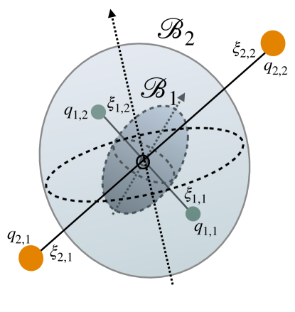
Let us first apply this to the case of the dynamics of coupled rigid bodies. The physical picture we have in mind consists of several rigid bodies attached rigidly in space at their centers of mass, but free to rotate about the centers of mass. They interact using, for example, electrostatic interaction. The physical problem is illustrated in Figure 1. The system consists of two rigid bodies , which can rotate freely about a common point in space. Each rigid body , , has a moment of inertia and contains several charges , , which are located in the coordinates in the body frame and are fixed with respect to that particular body or . Two charges on each body are shown in this illustration.
4.2 Equations of motion
The equations of motion for this system are found by specifying the general system (21) to the Lie group and taking the Hamiltonian of the coupled rigid bodies, given by the following expression:
| (30) |
see B for the derivation. These equations are given as:
| (31) | ||||
see (79) in B. Here, we have used the standard notation associating a antisymmetric matrix to a -vector in such a way that for any . In components, the hat map is
| (32) |
It is easy to verify from the last equation of (31) that , so if , then we have for all . This shows that if , then for all times.
For simulations, we take two charges on the body , positioned at , where and . The charges at are and the charges at are . The moments of inertia for the bodies are and .
4.3 Casimirs
Let us consider the more general system
| (33) | ||||
for an arbitrary Hamiltonian . Here, in our case, see (79) in B, but it could be an arbitrary internal force not necessarily coming from the derivative of with respect to .
Let us consider the quantity . Then we have
| (34) | ||||
Thus,
| (35) |
so the Casimir has the form
| (36) |
Physically, can be understood as the absolute value of the angular momentum seen from either the first or the second rigid body. This Casimir is a particular case of the class given in (74), applied to the Lie group .
4.4 Explicit expressions for the Poisson transformations and CLPNets
The algorithm defined in Section 3, which derives explicit expressions for transformations forming the neural network, proceeds as follows. Suppose we have data pairs, each one corresponding to the beginning and the end of the trajectory of length . At each time step, we have the initial and final angular momenta and the relative rotation at the initial and final point . We choose three sub-steps with the time allocated to each step to be , where is the total time difference between the steps.
-
Step 1.
Take the Hamiltonian to be for and . The equations of motion are:
(37) Remember that const during the motion. The evolution of is a rotation around the axis with a certain constant angular velocity given by . In order to compute the evolution equation for on the first step, let us investigate how the change in affects any vector . We compute:
(38) so rotates with a given angular velocity about , and thus the result of the rotation is the same as the rotation of . This consideration leads to the intermediary values
(39) where is the rotation matrix about the normalized axis by the angle .
Practical implementation: On each step, we choose three subsequent transformations: , where , are the basis vectors in the space of . Then, and the rotation matrices in (39) are simply rotations about the basis axes , . Each of the transformations corresponds to the choice of Hamiltonians
(40) where , and are parameters to be determined and is the activation function.
-
Step 2.
Take the Hamiltonian to be , for and . The equations of motion are:
(41) leading to the intermediary values
(42) where and with the linear operator mapping the initial to the final conditions of the linear ODE . In order to find this operator, we notice that the equation of motion for is just a rotation since at this step
(43) for any vector . So is rotating with a fixed angular velocity and thus
(44) We take since at the next step, there will be no more changes in .
Practical implementation: On each step, we choose three subsequent transformations: , so . Each of the transformations corresponds to the choice of Hamiltonians
(45) where, again, , and are parameters to be determined and is the activation function.
-
Step 3.
Since is a matrix, we take the following expression for the Hamiltonian :
(46) where all the indices run from to . The explicit form of the transformations for Step 3 is obtained directly from (28) as
(47)
4.5 Particular case of (31) with a common axis of rotation
Let us now consider the case when both rigid bodies rotate about a common axis, taken to be . This solution is possible if all charges are in the plane of both rigid bodies, and the axes for both rigid bodies are aligned with the axis of rotation . While this solution is indeed a specific solution of the equations (31), the application of CLPNets to this problem enables an understanding of how these particular transformations act.
The matrices are defined as rotations about the -axis:
| (48) |
where we have defined to be the relative angle. Since the rotations are about the axis, and are also parallel to the axis, the first terms on the right-hand sides of the first two equations of (31) vanish. All the applied forces are in the direction, and therefore all the torques are in the direction. Therefore, the equations of motion take the form
| (49) |
with being some torque. The indices above the variable denote which variable it refers to, and the subscript denotes the component of each variable. A little algebra shows that the equations can be cast into the form
| (50) |
with defined as
| (51) |
We can further simplify (50) as
| (52) |
By differentiating the -equation of the above system once, the equations reduce to a single equation for computed as
| (53) |
The rigid bodies can either rotate about the common axis if the initial momenta are high enough, or wobble around each other initially, so remains bounded. We shall now explore how to find the same reduced solution in the full space using CLPNets.
Remark 4.1 (On the canonical structure of the equations)
One could write (53) in the canonical form for the variables with and Hamiltonian , where . Thus, one could use the SympNets (Jin et al., 2020) to solve the canonical form of the system (53). However, this form is not generalizable to the arbitrary dynamics of coupled Lie group systems, so we will not use it here.
4.6 Applications of CLPNets to a particular solution of (31)
Note that we are going to use the data that were generated for the general system (31), and not the reduced system (52), as to test the ability of our method to find particular solutions of the equations.
-
1.
We test Hamiltonians of the type , with , and with being the activation function. Since the rotations about the axis commute with given by (48), the LPNets just changes the angle
(54) and leaves the momenta unchanged.
-
2.
We consider two matrices and with four parameters in each matrix:
(55) and the Hamiltonian:
(56) which is a particular case of (46) with a restricted form for and . Here , with being the chosen activation function, and thus
The evolution equation for this Hamiltonian leaves unchanged and modifies as follows:
(57) Thus, the adjustment of the value of momenta occurs in this step.
Note that the Casimir (36) is, in this case, given simply as and is conserved to machine precision.
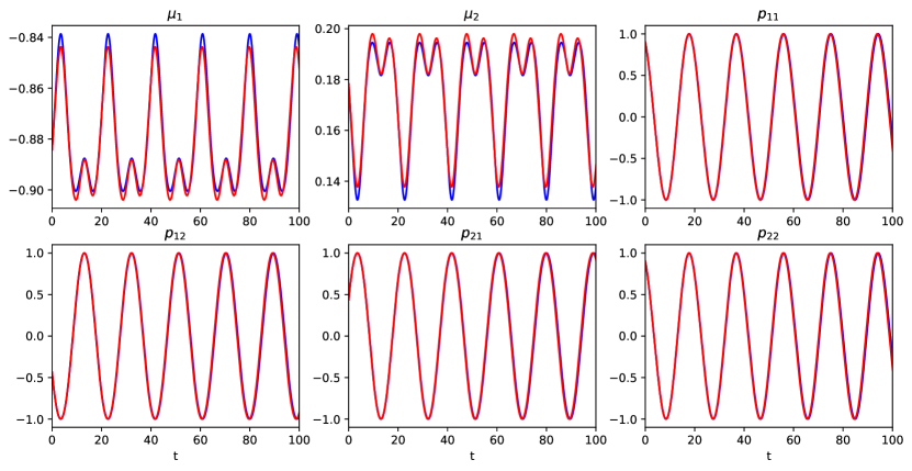
We present the results of the simulations of the vertical components of momenta and the meaningful components of the variables in Figure 2, for a simulation over 5000 steps ( with ). We used only 20 trajectories with 51 time steps each, i.e., 1000 data pairs, to learn the dynamics of the whole phase space. The initial conditions for , and the initial rotation angle for are chosen from a uniform random distribution in the interval for the angular momenta and for the angle. The initial trajectory for testing is chosen with initial momenta taken from a uniform distribution in the interval and an initial angle of relative rotation in the interval . The description of each rotation by the network involves three parameters. The terms in involve eight parameters, so each cycle contains 14 parameters. A network consisting of three repeated applications of these transformations involves 42 parameters. At the beginning of the learning procedure, all parameters are initialized randomly with a uniform distribution in the interval .
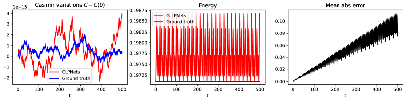
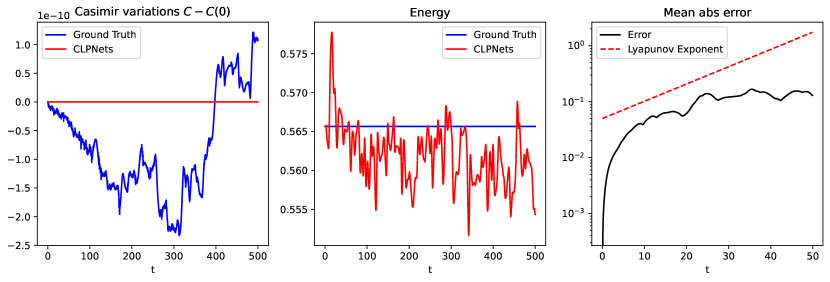
In Figure 3, we present the comparison of the Casimir from our solution vs the ground truth, the value of the energy, and the value of the mean absolute error. The Casimir is conserved to machine precision in both our case and the ground truth case obtained by the BDF algorithms. It is interesting that since the Casimir is a linear function, namely , it also happens to be conserved by the BDF algorithm. However, this is an exceptional case and is not true in general. The energy, while not being conserved as well as in the ground truth, remains oscillatory and is preserved well on average.
4.7 General dynamics for couple groups using CLPNets
The full three-dimensional motion described by equations (31) is not integrable and requires the full capability of our network, as defined by the substeps (39), (42) and (47).
-
1.
For the -rotation, we utilize rotations around the axis with the the Hamiltonian
(58) where , with being the activation function. The motion is simply the rotation about -axis by the angle .
-
2.
For the -rotation, we take
(59)
where, as usual, and is the activation function. The CLPNets are applied in the following sequence: first, as given by (58), then using the same formula, and finally as described by (46). This sequence of cycles is repeated times at each time step.
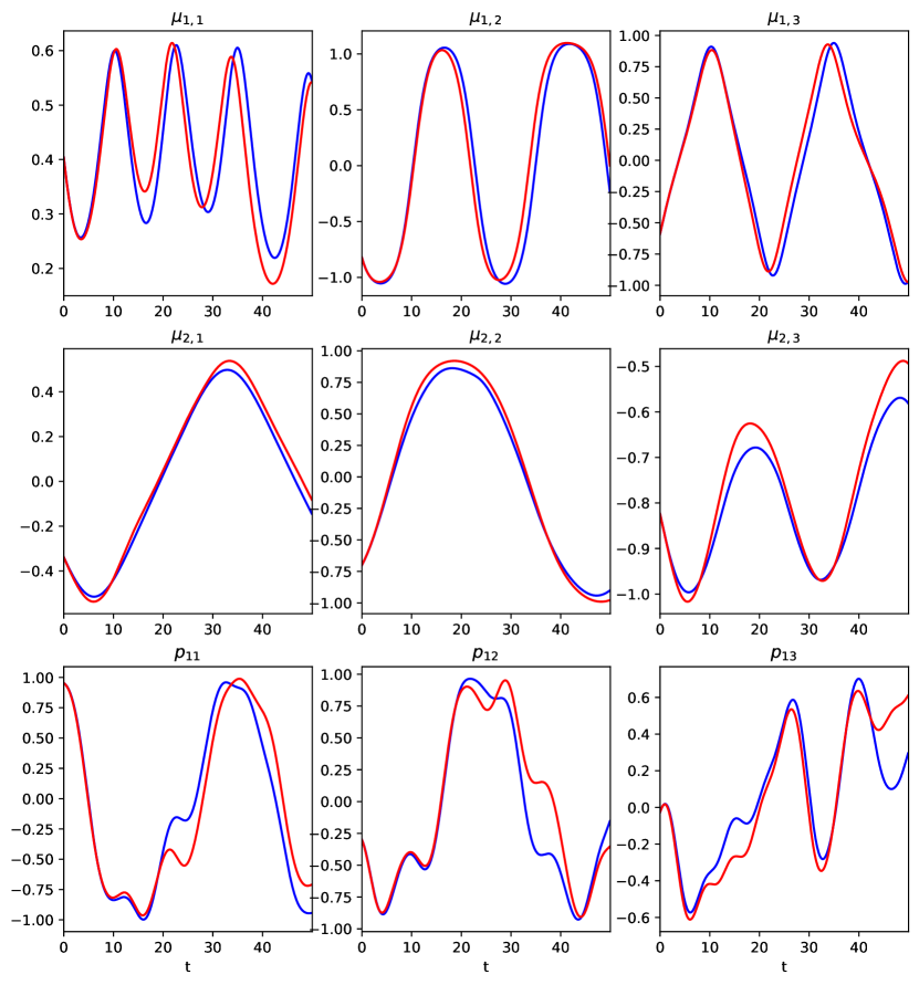
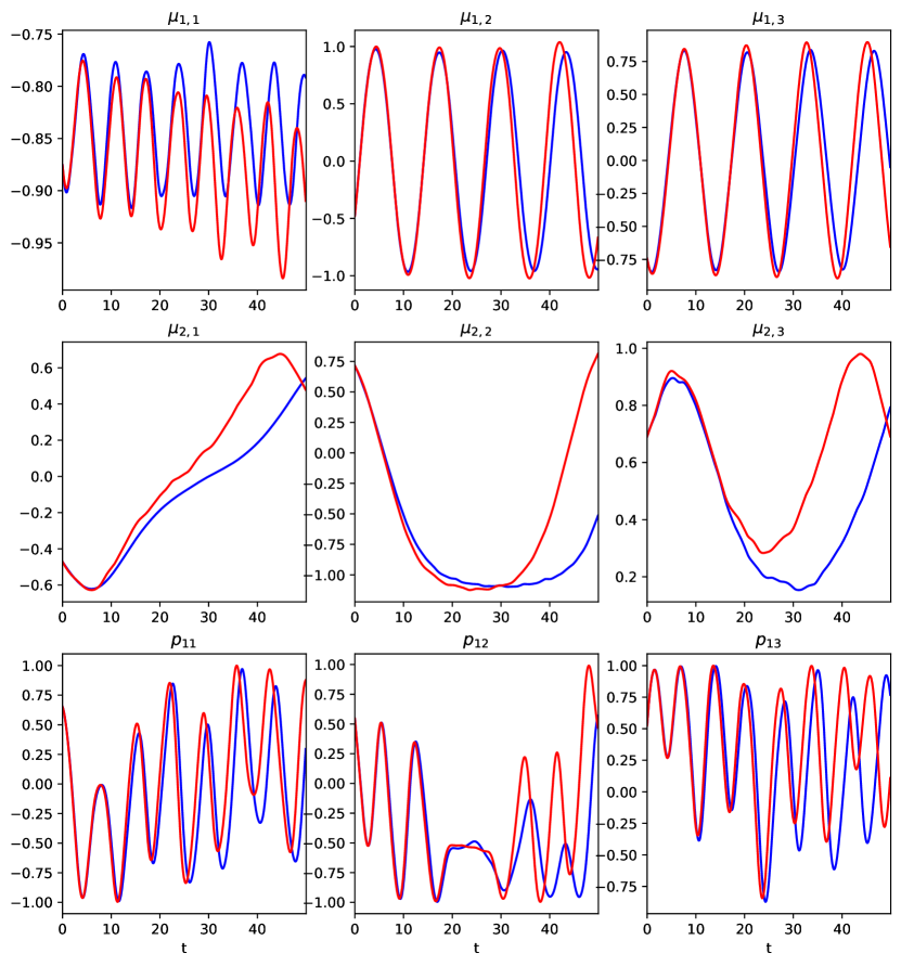
The learning is obtained from 20 trajectories of 51 points each, corresponding to 1000 data pairs. Note that this is exactly the same number of data points as the reduced case described above; however, the case is effectively -dimensional, whereas the case of full coupled rotations is -dimensional. The initial conditions for these trajectories are chosen at random in a cube of size , so , and are each taken from a random distribution on the interval , while the corresponding initial value of is obtained as a rotation matrix about a random unit vector, with an angle randomly chosen in the interval . The total number of parameters of the network in this setting is 108. At the beginning of the learning procedure, all parameters are initialized randomly with a uniform distribution in the interval . The Adam algorithm is performed for optimization. The loss, taken to be MSE of all components, is reduced from about to after 2000 epochs in the realization shown. The initial learning rate is , decreasing exponentially to . The results of simulations and their comparison with the ground truth are shown in Figure 4.
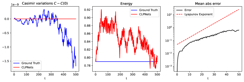
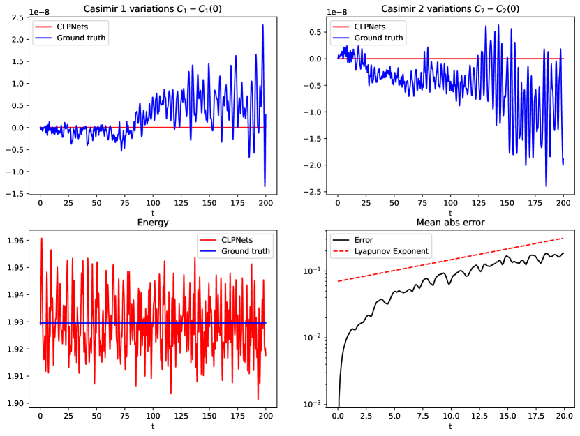
The conservation of Casimirs and energy by the ground truth simulation vs our data is shown on the left and central panels of Figure 5, respectively. Note that the Casimir is preserved by our method with machine precision, better than the ground truth. In contrast, the energy is conserved less accurately than the ground truth. For some initial conditions, the preservation of energy is quite accurate on average, although in the case presented here, the error in energy grows approximately linearly in time. Since the solution of equations (31) are generally chaotic, the distance between nearby trajectories that are initially close diverges exponentially with time , where is the (leading) Lyapunov exponent. We measure the value of the Lyapunov exponent from direct simulations. The growth of error proportional to is the lowest one can expect in chaotic systems. The growth of mean absolute error (MAE) is demonstrated on the right panel of Figure 5 as a solid black line, along with the dashed line showing exponential growth according to the Lyapunov exponent .
4.8 Results for more general Hamiltonians
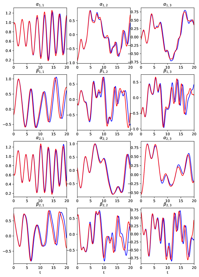
In the Hamiltonian (30), we used the functional form of the sum of squares of momenta, dictated by physical arguments. To demonstrate that our method is applicable to general Hamiltonians, we simulated the equations with an altered (unphysical) Hamiltonian , where is a parameter and is given by (30). Note that each individual trajectory of this new system is obtained by a rescaling in the original system (31). However, the time scale depends on the value of that trajectory’s Hamiltonian, so the phase flow mapping in the phase space deforms compared to the original system, while still remaining a Poisson transformation. The Casimir is, of course, independent of the Hamiltonian and is still given by the expression (36). We present the results of our simulations for , showing the values of momenta and orientations in Figure 6, and the conservation of the Casimir, energy, and error growth in Figure 7. The results for are very similar to those shown in Figures 4 and 5, with the loss converging to small values, typically about , within 2000 epochs. This demonstrates that our algorithm can also handle more complex functional forms of the Hamiltonians. For larger , such as , the convergence appears to worsen, with the loss, while decaying, remaining at around after 2000 epochs, which is about ten times worse than for smaller values of . We attribute this loss of accuracy to large variations in the potential energy terms in (30) due to the dynamics of electrostatic charges. These variations cause significant slowdowns or speedups in solutions with the Hamiltonian compared to the original Hamiltonian in (30). This discrepancy in time scales is challenging to capture with the regular activation functions considered here. Due to the lack of physical relevance of this type of Hamiltonian and the challenging nature of the question of capturing dynamics in phase space with different time scales using a neural network, we do not pursue this line of thought further here and defer the discussion to future work on the subject.
5 Coupled systems on : rotational and translational dynamics
5.1 Lie group definitions, operators and equations of motion
We now proceed to the consideration of equations of motion for the Lie group of rotations and translations, which is important for the computation of discretization of elastic bodies, such as geometrically exact rods (Demoures et al. (2015); Gay-Balmaz and Putkaradze (2016)). This case is the most complex example we will consider.
We start with some definition of the semidirect product group of rotations and translations . For a rotation and translation , we form a matrix , with corresponding multiplication and inverse
| (60) |
where is the row of zeros. The momenta of are six-dimensional and consist of three-dimensional angular momenta and linear momenta . Thus, the evolution equation in the Hamiltonian representation contains the variables and the relative orientation and position . The equations of motion are derived from the general expression (21) in C. They are given as follows:
| (61) |
We choose the following Hamiltonian to compute the training data for (61):
| (62) | ||||
with the tensors of inertia , , the masses , and the tensors and associated with the potential energy.
5.2 CLPNets for dynamics
For the Lie group , the algorithm defined in Section 3 proceeds via the following 6 steps.
-
Step 1.
Take the Hamiltonian to be , for . One can readily see that const. Denoting, as usual, by the rotation matrix with unit axis and angle , the equations of motion are
(63) Here we defined as before .
Practical implementation: On each step, we choose three subsequent transformations: , where , are the basis vectors in the space. Again, just as in (39), the rotation matrices in (63) are simply rotations about the basis axes in the space, with . Each of the transformations corresponds to the choice of Hamiltonians
(64) where , , and are parameters to be determined and is the activation function.
-
Step 2.
Take the Hamiltonian to be , for . One can again readily see that const. The equations of motion for this step are
(65) Practical implementation: Similarly to Step 1, we take three sequential sub-steps with the choice of vectors . Then, we choose
where , and are parameters to be determined and is the activation function.
-
Step 3.
Take the Hamiltonian to be , for . The equations of motion are
(66) with .
Practical implementation: Similarly to Step 1, we choose three subsequent transformations: , where , are the basis vectors in the space. Then, . Again, just as in (39), the rotation matrices in (63) are simply rotations about the basis axes in the space, with . Each of the transformations corresponds to the choice of Hamiltonians
(67) where , and are parameters to be determined and is the activation function.
-
Step 4.
Take the Hamiltonian to be , for . The equations of motion are
(68) Practical implementation: Similarly to Step 2, we take three sequential sub-steps with . Then, we choose
where , and are parameters to be determined and is the activation function.
-
Step 5.
Take the Hamiltonian to be . The equations of motion are
(69) Practical implementation: For , we choose the neural network parameterization exactly as in (59), since we are describing the rotational part of the group.
-
Step 6.
Take the Hamiltonian to be . The equations of motion are
(70) Practical implementation: We take three sub-steps defined by some functions , . Then, we choose
where , and are some constants and is the activation function.
Note that steps 5 and 6 above can be combined into a single step since the equations for these Hamiltonians are explicitly solvable.
5.3 Results of application of CLPNets algorithm for the whole space learning
The results of the simulations are presented in Figure 8, showing the angular and linear momenta , , which exhibit reasonable agreement. The learning was conducted with 1000 data pairs, coming from trajectories of length data points each, with initial conditions randomly positioned in phase space. Specifically, the initial conditions for the trajectory data pairs are chosen randomly within the cube , ; the initial rotation for the data pair is a rotation about a random axis with an angle randomly selected in the interval , and the initial conditions for are also chosen randomly within the cube . All random distributions are uniform. The ground truth solutions are computed using a high-precision BDF algorithm for .
The CLPNets algorithm is comprised of transformations of types 1-6 described above. The sequence of transformations performed is . This sequence is repeated three times, resulting in a total of 189 parameters. The Adam algorithm is used for optimization, resulting in a reduction of the loss, which is taken to be the Mean Square Error (MSE), from about to in 2000 epochs for the example shown here. The initial learning rate is chosen to be , decreasing exponentially to by the end of the learning procedure. The values of all parameters of the neural network are initialized randomly with a uniform distribution in the range .
After the learning is completed, we perform simulations starting with a random initial point, which we have chosen at random in a cube , ; the initial rotation for the data pair is again taken to be a rotation about a random axis with an angle randomly chosen in the interval , and initial conditions for are chosen randomly from the cube . Thus, this particular trajectory was never observed by the system during learning, and our algorithm is capable of learning the dynamics in the whole phase space.
Remark 5.1 (On resisting the curse of dimensionality by CLPNets)
We remind the reader that the phase space for the coupled system considered here is 18-dimensional, with each momentum belonging to a linear space of dimension 6, and the group elements also described by 6 parameters. It is thus even more surprising that the dynamics of the whole phase space can be described by such a low number of data points. Thus, one can say that our method resists the curse of dimensionality. We conjecture that the method can be highly computationally efficient for higher-dimensional problems, such as those arising from the discretization of realistic elasticity models.
While we do not observe a perfect match like we did for some simpler integrable systems, we note that since the system is chaotic, a perfect match should not be expected. On Figure 9, we show the results of the conservation of the Hamiltonian and the Casimir (left panel) and the error growth vs Lyapunov’s exponent (right panel). The error growth matches the results of Lyapunov’s exponent, which is the best result one can hope to achieve for the prediction of a chaotic system.
While the results on Figure 8 and Figure 9 do not show perfect matching expected for more simple systems, we remind the reader that the learning was done on an 18-dimensional manifold using only 189 parameters and 1000 data points. Thus, we find the application of CLPNets to the coupled system to be quite effective.
On the top part of the figure, we present the conservation of two Casimirs for the system. They are obtained from the general class of Casimirs given in Lemma from A.1 following (Krishnaprasad and Marsden, 1987): if is a Casimir of the motion on just the Lie algebra part of the dynamics, then is a Casimir for the extended part of the dynamics. In our case, if is a Casimir of the -dynamics, then will be the corresponding Casimir for the full dynamics.
5.4 Casimirs
The regular Lie-Poisson motion on has two Casimirs, as is well established in the corresponding theory related to Kirchhoff’s equations modeling underwater vehicles (Leonard and Marsden, 1997; Holmes et al., 1998). In terms of the angular and linear momenta, these two Casimirs are written as and . The general formula (74) yields two Casimirs for the coupled bodies:
| (71) |
These Casimirs are plotted in the top panels of Figure 9. Once again, the Casimirs in our scheme are conserved with machine precision, whereas the Casimirs provided by the ground truth are only conserved up to accuracy. In the bottom panels, we plot the energy conservation (left panel) and the growth of error (right panel). We see that the energy is conserved by our scheme with less precision than the ground truth, as expected, although the energy in this particular case is conserved quite well on average. Additionally, the growth of MAE in all components is consistent with the expected best case given by the Lyapunov exponent. The exact nature of conservation and growth of errors in components and energy depends on the specific point chosen in the phase space, but the Casimirs in our case are always conserved with machine precision, much better than the ground truth solutions.
6 Conclusions and future work
In this paper, we have derived a novel algorithm – CLPNets – that is capable of learning the whole space dynamics (more precisely, the dynamics of a large portion of the phase space) for systems containing several interacting parts. The learning procedure involves constructing a network from a sequence of transformations with parameters. These transformations, derived from specific functional forms of test Hamiltonians and taken in sequence, faithfully reproduce the structure of dynamics in the phase space. We demonstrate that learning the dynamics in phase space requires only a modest number of data points, and the network includes a relatively small number of parameters, even when the system’s total dimension is high. The efficient operation of the CLPNets network enables future expansion of this method to compute highly efficient, structure-preserving, data-based solutions to challenging problems, such as those in nonlinear elasticity and continuum mechanics. In particular, in follow-up work, we will study a model of an elastic rod, which consists of a chain of coupled elements as described in Section 5. It will also be interesting to see if alternative data-based, structure-preserving methods suggested recently (Vaquero et al., 2023, 2024) can offer similar performance for the higher-dimensional coupled systems considered here.
7 Acknowledgements
We are grateful to Anthony Bloch, Pavel Bochev, Eric Cyr, David Martin de Diego, Sofiia Huraka, Justin Owen, Brad Theilman, and Dmitry Zenkov for fruitful and engaging discussions. FGB was partially supported by a start-up grant from the Nanyang Technological University. VP was partially supported by the NSERC Discovery grant.
This article has been co-authored by an employee of National Technology & Engineering Solutions of Sandia, LLC under Contract No. DE-NA0003525 with the U.S. Department of Energy (DOE). The employee owns right, title, and interest in and to the article and is responsible for its contents. The United States Government retains and the publisher, by accepting the article for publication, acknowledges that the United States Government retains a non-exclusive, paid-up, irrevocable, world-wide license to publish or reproduce the published form of this article or allow others to do so, for United States Government purposes. The DOE will provide public access to these results of federally sponsored research in accordance with the DOE Public Access Plan https://www.energy.gov/downloads/doe-public-access-plan.
References
- Amirouche (1986) Amirouche, M., 1986. Dynamic analysis of ‘tree-like’structures undergoing large motions–a finite segment approach. Engineering analysis 3, 111–117.
- Antman (2005) Antman, S.S., 2005. General theories of rods. Nonlinear Problems of Elasticity , 603–658.
- Arnol’d (2013) Arnol’d, V.I., 2013. Mathematical Methods of Classical Mechanics. volume 60. Springer Science & Business Media.
- Bajārs (2023) Bajārs, J., 2023. Locally-symplectic neural networks for learning volume-preserving dynamics. Journal of Computational Physics 476, 111911.
- Banavar et al. (2007) Banavar, J.R., Hoang, T.X., Maddocks, J.H., Maritan, A., Poletto, C., Stasiak, A., Trovato, A., 2007. Structural motifs of biomolecules. Proceedings of the National Academy of Sciences 104, 17283–17286.
- Baydin et al. (2018) Baydin, A.G., Pearlmutter, B.A., Radul, A.A., Siskind, J.M., 2018. Automatic differentiation in machine learning: a survey. J. of Mach. Learn. Research 18, 1–43.
- Bi et al. (2023) Bi, K., Xie, L., Zhang, H., Chen, X., Gu, X., Tian, Q., 2023. Accurate medium-range global weather forecasting with 3d neural networks. Nature , 1–6.
- Burby et al. (2020) Burby, J.W., Tang, Q., Maulik, R., 2020. Fast neural Poincaré maps for toroidal magnetic fields. Plasma Physics and Controlled Fusion 63, 024001.
- Calhoun et al. (2019) Calhoun, M.A., Bentil, S.A., Elliott, E., Otero, J.J., Winter, J.O., Dupaix, R.B., 2019. Beyond linear elastic modulus: viscoelastic models for brain and brain mimetic hydrogels. ACS Biomaterials Science & Engineering 5, 3964–3973.
- Chen and Tao (2021) Chen, R., Tao, M., 2021. Data-driven prediction of general Hamiltonian dynamics via learning exactly-symplectic maps, in: International Conference on Machine Learning, PMLR. pp. 1717–1727.
- Chen et al. (2020) Chen, Z., Zhang, J., Arjovsky, M., Bottou, L., 2020. Symplectic recurrent neural networks. International Conference on Learning Representations .
- Chirikjian (1994) Chirikjian, G.S., 1994. Hyper-redundant manipulator dynamics: A continuum approximation. Advanced Robotics 9, 217–243.
- Cranmer et al. (2020) Cranmer, M., Greydanus, S., Hoyer, S., Battaglia, P., Spergel, D., Ho, S., 2020. Lagrangian neural networks. arXiv preprint arXiv:2003.04630 .
- Cuomo et al. (2022) Cuomo, S., Di Cola, V.S., Giampaolo, F., Rozza, G., Raissi, M., Piccialli, F., 2022. Scientific machine learning through physics-informed neural networks: Where we are and what’s next. arXiv preprint arXiv:2201.05624 .
- David and Méhats (2021) David, M., Méhats, F., 2021. Symplectic learning for Hamiltonian neural networks. arXiv preprint arXiv:2106.11753 .
- Demoures et al. (2015) Demoures, F., Gay-Balmaz, F., Leyendecker, S., Ober-Blöbaum, S., Ratiu, T.S., Weinand, Y., 2015. Discrete variational Lie group formulation of geometrically exact beam dynamics. Numerische Mathematik 130, 73–123.
- Dubinkina and Frank (2007) Dubinkina, S., Frank, J., 2007. Statistical mechanics of Arakawa’s discretizations. Journal of Computational Physics 227, 1286–1305. URL: https://www.sciencedirect.com/science/article/pii/S0021999107003944, doi:https://doi.org/10.1016/j.jcp.2007.09.002.
- Eldred et al. (2024) Eldred, C., Gay-Balmaz, F., Huraka, S., Putkaradze, V., 2024. Lie-Poisson neural networks (LPNets): Data-based computing of Hamiltonian systems with symmetries. Neural Networks , 106162.
- Ellis et al. (2010) Ellis, D.C., Gay-Balmaz, F., Holm, D.D., Putkaradze, V., Ratiu, T.S., 2010. Symmetry reduced dynamics of charged molecular strands. Archive for rational mechanics and analysis 197, 811–902.
- Gay-Balmaz et al. (2012) Gay-Balmaz, F., Holm, D.D., Putkaradze, V., Ratiu, T.S., 2012. Exact geometric theory of dendronized polymer dynamics. Advances in Applied Mathematics 48, 535–574.
- Gay-Balmaz and Putkaradze (2016) Gay-Balmaz, F., Putkaradze, V., 2016. Variational discretizations for the dynamics of fluid-conveying flexible tubes. Comptes Rendus Mécanique 344, 769–775.
- Greydanus et al. (2019) Greydanus, S., Dzamba, M., Yosinski, J., 2019. Hamiltonian neural networks. Advances in neural information processing systems 32.
- Hall and Leok (2015) Hall, J., Leok, M., 2015. Spectral variational integrators. Numerische Mathematik 130, 681–740.
- Han et al. (2021) Han, C.D., Glaz, B., Haile, M., Lai, Y.C., 2021. Adaptable Hamiltonian neural networks. Physical Review Research 3, 023156.
- Holmes et al. (1998) Holmes, P., Jenkins, J., Leonard, N.E., 1998. Dynamics of the Kirchhoff equations i: Coincident centers of gravity and buoyancy. Physica D: Nonlinear Phenomena 118, 311–342.
- Ider and Amirouche (1989) Ider, S., Amirouche, F., 1989. Influence of geometric nonlinearities in the dynamics of flexible treelike structures. Journal of Guidance, Control, and Dynamics 12, 830–837.
- Jiang et al. (2015) Jiang, Y., Li, G., Qian, L.X., Liang, S., Destrade, M., Cao, Y., 2015. Measuring the linear and nonlinear elastic properties of brain tissue with shear waves and inverse analysis. Biomechanics and modeling in mechanobiology 14, 1119–1128.
- Jin et al. (2022) Jin, P., Zhang, Z., Kevrekidis, I.G., Karniadakis, G.E., 2022. Learning Poisson systems and trajectories of autonomous systems via Poisson neural networks. IEEE Transactions on Neural Networks and Learning Systems .
- Jin et al. (2020) Jin, P., Zhang, Z., Zhu, A., Tang, Y., Karniadakis, G.E., 2020. SympNets: Intrinsic structure-preserving symplectic networks for identifying Hamiltonian systems. Neural Networks 132, 166–179.
- Karniadakis et al. (2021) Karniadakis, G.E., Kevrekidis, I.G., Lu, L., Perdikaris, P., Wang, S., Yang, L., 2021. Physics-informed machine learning. Nature Reviews Physics 3, 422–440.
- Kim and Lee (2024) Kim, D., Lee, J., 2024. A review of physics informed neural networks for multiscale analysis and inverse problems. Multiscale Science and Engineering , 1–11.
- Krishnaprasad and Marsden (1987) Krishnaprasad, P.S., Marsden, J.E., 1987. Hamiltonian structures and stability for rigid bodies with flexible attachments. Archive for Rational Mechanics and Analysis 98, 71–93.
- Krishnapriyan et al. (2021) Krishnapriyan, A., Gholami, A., Zhe, S., Kirby, R., Mahoney, M.W., 2021. Characterizing possible failure modes in physics-informed neural networks. Advances in Neural Information Processing Systems 34, 26548–26560.
- Leok and Shingel (2012) Leok, M., Shingel, T., 2012. General techniques for constructing variational integrators. Frontiers of Mathematics in China 7, 273–303.
- Leonard and Marsden (1997) Leonard, N.E., Marsden, J.E., 1997. Stability and drift of underwater vehicle dynamics: mechanical systems with rigid motion symmetry. Physica D: Nonlinear Phenomena 105, 130–162.
- Marsden and Ratiu (2013) Marsden, J., Ratiu, T., 2013. Introduction to Mechanics and Symmetry: a basic exposition of classical mechanical systems. volume 17. Springer Science & Business Media.
- Marsden et al. (1999) Marsden, J.E., Pekarsky, S., Shkoller, S., 1999. Discrete Euler–Poincaré and Lie–Poisson equations. Nonlinearity 12, 1647.
- Marsden and West (2001) Marsden, J.E., West, M., 2001. Discrete mechanics and variational integrators. Acta numerica 10, 357–514.
- Mengaldo et al. (2022) Mengaldo, G., Renda, F., Brunton, S.L., Bächer, M., Calisti, M., Duriez, C., Chirikjian, G.S., Laschi, C., 2022. A concise guide to modelling the physics of embodied intelligence in soft robotics. Nature Reviews Physics 4, 595–610.
- Mihai et al. (2017) Mihai, L.A., Budday, S., Holzapfel, G.A., Kuhl, E., Goriely, A., 2017. A family of hyperelastic models for human brain tissue. Journal of the Mechanics and Physics of Solids 106, 60–79.
- Nieuwenhuis et al. (2018) Nieuwenhuis, R., Kubota, M., Flynn, M.R., Kimura, M., Hikihara, T., Putkaradze, V., 2018. Dynamics regularization with tree-like structures. Applied Mathematical Modelling 55, 205–223.
- Pathak et al. (2022) Pathak, J., Subramanian, S., Harrington, P., Raja, S., Chattopadhyay, A., Mardani, M., Kurth, T., Hall, D., Li, Z., Azizzadenesheli, K., et al., 2022. Fourcastnet: A global data-driven high-resolution weather model using adaptive Fourier neural operators. arXiv preprint arXiv:2202.11214 .
- Raissi et al. (2019) Raissi, M., Perdikaris, P., Karniadakis, G.E., 2019. Physics-informed neural networks: A deep learning framework for solving forward and inverse problems involving nonlinear partial differential equations. Journal of Computational physics 378, 686–707.
- de Rooij and Kuhl (2016) de Rooij, R., Kuhl, E., 2016. Constitutive modeling of brain tissue: current perspectives. Applied Mechanics Reviews 68, 010801.
- Simo et al. (1988) Simo, J.C., Marsden, J.E., Krishnaprasad, 1988. The hamiltonian structure of nonlinear elasticity: The material and convective representation of solids, rods, and plates. Archive for Rational Mechanics and Analysis 104, 125–183.
- Šípka et al. (2023) Šípka, M., Pavelka, M., Esen, O., Grmela, M., 2023. Direct Poisson neural networks: Learning non-symplectic mechanical systems. arXiv preprint arXiv:2305.05540 .
- Tao (2016) Tao, M., 2016. Explicit symplectic approximation of nonseparable Hamiltonians: Algorithm and long time performance. Physical Review E 94, 043303.
- Vaquero et al. (2023) Vaquero, M., Cortés, J., de Diego, D.M., 2023. Symmetry preservation in Hamiltonian systems: Simulation and learning. arXiv preprint arXiv:2308.16331 .
- Vaquero et al. (2024) Vaquero, M., de Diego, D.M., Cortés, J., 2024. Designing Poisson integrators through machine learning. arXiv preprint arXiv:2403.20139 .
- Xiong et al. (2020) Xiong, S., Tong, Y., He, X., Yang, S., Yang, C., Zhu, B., 2020. Nonseparable symplectic neural networks. arXiv preprint arXiv:2010.12636 .
Appendix A Mathematical background on the dynamics of coupled bodies
A.1 Notations for systems on Lie groups
We quickly explain here the notations used throughout the paper for the treatment and derivation of the equations of motion for systems on Lie groups.
Let us denote by , the action by conjugation. The adjoint action is , defined by with a curve tangent to at and the Lie algebra of . The Lie bracket is found as , for , with the same curve as before. Given a duality pairing between and its dual , the coadjoint action is , defined by , for all and . Then, the coadjoint operator appearing in the equations (16), (17), (21) is defined by
and satisfies .
Given a Lagrangian as in (18), its partial derivatives and are defined by
with a curve with and where the duality pairing is between the tangent and cotangent spaces and at . The expression appearing in equations (16) and (17) is defined by
| (72) |
with defined by with a curve with and . The partial derivatives and appearing in (21) are defined similarly.
A.2 Poisson brackets, Casimirs functions, and symplectic leaves
We recall that Poisson brackets on a manifod are bilinear skewsymmetric maps satisfying the Leibniz rule and the Jacobi identity , for all . The fact that the bracket (22) for coupled systems defines a Poisson bracket on follows from Poisson reduction by symmetry of the canonical Poisson bracket on . More precisely, the quotient map
associated to the left action of on , relates the bracket (22) to the canonical Poisson bracket on as follows:
From this and general results in Poisson reduction, it immediately follows that (22) is a Poisson bracket, see Marsden and Ratiu (2013).
Due to its non-canonical nature, this bracket admits Casimir functions, i.e. functions which satisfy
A class of Casimir functions is given in the following Lemma, in which we also consider the Lie-Poisson bracket on given by
| (73) |
for . Recall that this bracket also emerges by Poisson reduction, in the simpler situation of the quotient map
associated to the left action of on .
Lemma A.1
Let be a Casimir function of the Lie-Poisson bracket on , i.e.,
Then the function defined by
| (74) |
is a Casimir function for the Poisson bracket (22).
Proof. As a Casimir for (73), the function satisfies
| (75) |
The partial derivatives of are
where we used (75) in the last equality, as well as the formulas
for the variatons with respect to . Inserting these expressions in (22), we get
where we used (75) in the last equality, with .
The class of Casimir functions given in (74) is a particular case of the class considered in (Krishnaprasad and Marsden, 1987) for coupled systems.
Finally, from a general result on Poisson structures, it follows that the phase space of the Poisson bracket (22) is foliated into symplectic leaves, on which the flow of the Hamiltonian system (21) restricts and becomes symplectic, Marsden and Ratiu (2013). More precisely, given a symplectic leaf , there exists a unique symplectic form on such that the Poisson bracket, when restricted to , becomes associated to the symplectic form :
where is the Hamiltonian vector field associated to the function on the symplectic manifold , i.e. . Note that Casimir functions are constant on symplectic leaves.
As we have shown, the CLPNets algorithms preserve the symplectic leaves and hence the Casimir functions.
Appendix B Derivation of the equations of motion for two coupled rigid bodies
Notations and preliminaries
The Lie group to be considered in this case is with Lie algebra given by antisymmetric matrices. We identify the dual with by using the duality pairing , , . We further identify antisymmetric matrices with vectors by using the hat isomorphism , , defined by , for all . The inverse is written , satisfying , for all . With this identification, we have
| (76) |
The operator is extended from to arbitrary matrices , by considering its skewsymmetric part as follows , for all . With this extension, we have the identity
| (77) |
which will be used below. The pairing between and is
| (78) |
and is left and right invariant. With this setting, by specifying the general equations (21) to the group or rotations, we get:
| (79) |
Physical system and equations of motion
The physical setup of the problem is as follows. Let us consider two rigid bodies with their fixed point coinciding at . Each of the rigid bodies and has charges of value , with the coordinates in each body frame. If the orientation of each rigid body is given by , then the distance between the charges (body 1) and (body 2) are
| (80) |
Assuming the tensors of inertia for each of the rigid body are , the physical Hamiltonian of this problem is given by
| (81) |
The computations of the derivatives proceed as follows:
| (82) |
where we recall that we use the pairing (78). Then from (77) and using , we get
| (83) | ||||
Clearly, the force from charges acting on the first rigid body is the negative of the force acting on the second rigid body, multiplied by , as expected. Substituting (82) and (83) into (79), we obtain the final equations of motion for two coupled rigid bodies (31).
Appendix C Derivation of equations of motion for two coupled bodies
The coadjoint action is computed following the definition in A.1. For any two elements , we have
| (84) |
The -action is computed by considering a curve at the identity and taking the derivative at . If we denote , then
| (85) | ||||
where we have defined the element of the Lie algebra by two components, collecting the meaningful non-zero terms in the matrix. Note that since , (85) can be written equivalently in vector form
| (86) |
The -action is then computed by additionally by considering and taking the derivative of that quantity at . Again, with , we obtain, in the matrix and vector forms, respectively:
| (87) | ||||
Let us consider the pairing between an element and a dual element defined by
| (88) |
Then, with (88), we can derive the expression for the coadjoint action as follows:
| (89) | ||||
| (90) |
We now compute the variations with respect to in order to derive the terms coming from the partial derivative in the equations of motion for . Denote the variations as , where and are angular and linear momentum variations, respectively. We proceed as follows:
| (91) | ||||
The terms proportional to yield the terms in the equation for , while those proportional to contribute to the equation for .