Hybrid Type-II and Type-III seesaw model for the muon anomaly
Abstract
In this work, we investigate the muon anomalous dipole moment in a model that extends the Standard Model with a scalar triplet and a vector-like lepton triplet. Different from previous studies, we find that there is still viable parameter space in this model to explain the discrepancy . While being consistent with the current data of neutrino mass, precision electroweak measurements and the perturbativity of couplings, our model can provide new physics contribution to cover the central region of with new scalar and fermion mass as low as around TeV. This mass scale is allowed by the current collider searches for doubly charged scalars and vector-like leptons, and they can be tested at future high energy and/or high luminosity colliders.
I Introduction
The anomalous magnetic moment (AMM) of muon, denoted as , has been theoretically predicted in the Standard Model (SM) and experimentally measured both to very high precision. Since the experiment E821 performed at Brookhaven National Laboratory (BNL) released its data about two decades ago [1], a discrepancy has been existing and triggered rich phenomenological studies (see review [2, 3] and and references therein). Recently, on the theoretical side, a comprehensive summary of the most accurate SM prediction for is provided in [4] where the value is reported as . On the experimental side, the Muon Experiment at Fermilab released its Run-1 dataset in 2021 and the experimental result was [5] when combining the data from Fermilab Run-1 and BNL. This resulted in a deviation from the SM prediction of with a significance of . In 2023, Fermilab released data from Run-2 and Run-3 leading to a new result after being combined with Run-1 and the BNL data as [5]. In this case the deviation from the SM prediction achieved a significance of . These results inspired phenomenological investigations in various new physics models [6, 7, 8, 9] 111Recently, there have been some discussions on the discrepancies in the calculation of the hadronic vacuum polarization contribution to between the lattice QCD calculations and experimental data in measurements of , which seems to reduce to some extend [10, 11, 12]. .
In the framework of simplified models, contributions to can be generated at the 1-loop level by introducing several new physics fields with various spins and quantum numbers under the electroweak gauge group . For discussions involving one, two, or three new fields, see the recent reviews [13, 14, 15, 16] and the references therein. The chiral structure of the can be described by the following effective tensor operator
| (1) |
in which the SM charged lepton should be understood as muon flavor. We can see that both the left-handed (LH) and the right-handed (RH) of muon are involved. More specifically, if one considers the new physical contribution to at 1-loop level, proper chiral flip is needed along the fermion line. This chiral flip can take place either in the external muon line realized by the SM Yukawa interaction outside the loop or in the internal fermion line inside the loop [15].
To explain it generally requires either new fields with light masses to avoid too much loop suppression or heavy particles inside the loop to generate chiral enhancement to the amplitude. However, light new fields are often constrained by electroweak precision observables, flavor physics, and collider searches, typical examples of which include the two-Higgs-doublet model [17] and the dark photon model [18]. Given the aformentioned experimental constraints many models are viable only in the parameter space where the new particles are heavy. Therefore, proper chiral enhancement is typically necessary to adequately explain .
As pointed out in recent reviews [13, 16], many models fail to explain either due to the absence of chiral enhancement or the wrong sign of in the prediction (e.g. minimal seesaw models [19, 20]). Chiral enhancement can be achieved, for instance, through a chiral flip occurring on a fermionic field within the loop as manifested in supersymmetric models [21, 22]. These fermionic fields can also appear as charm/top quark in SM or vector-like quarks in leptoquark-extended models [23, 24, 25], or more generally as new physics fermions being Dirac, Majorana, or Weyl nature.
It has been found in recent studies [14, 15, 16] that simplified models introducing two new fields with different spins to the SM are unable to generate the necessary chiral enhancement within the 1-loop structure of . As a result, these models tend to confine the new particles to a low and compressed mass region in order to explain while avoiding collider constraints. However, an important consideration has been overlooked in the aforementioned analyses: the Yukawa interaction involving the SM Higgs doublet and the newly introduced fermion. The Yukawa interaction, a four-dimensional operator, naturally exists and can induce mass mixing between fermions in the SM and the new physics sector.
In this work, we demonstrate that by incorporating the SM Higgs Yukawa interaction into the analysis, simplified models introducing two new fields to the SM can effectively explain . As a concrete example, we consider a simplified model that extends the SM with a scalar triplet and a vector-like lepton (VLL) triplet under the electroweak gauge group . These two particles have been scrutinized in neutrino mass generation mechanisms as Type-II [26, 27, 28, 29, 30, 31] and Type-III [32, 33] seesaw models, respectively. However, in this work concentrating on the physics of , we do not require our model to produce the experimentally suggested texture of neutrino mass matrix, but instead ensure the theoretically predicted neutrino mass remains to be negligibly small and close to zero.
II Model setup and parameters
II.1 Model setup
In our model we extend the SM with a scalar triplet and a vector-like lepton (VLL) triplet , of which the representation under the SM electroweak gauge group are
| (2) |
and the component fields are
| (7) |
We consider the following mass and Yukawa terms in the Lagrangian which are most relevant to the physics of
| (8) | ||||
in which is the SM scalar doublet and () is the LH (RH) lepton doublet (singlet) in SM with denoting the generation index. denotes the charge conjugation of the field satisfying with . Note that in our notation the operator also acts on the representation space of SM gauge group.
After performing the expansion we can derive the following neutrino and charged lepton mass matrices
| (9) | ||||
Then, the Yukawa interactions can be written as
| (10) | ||||
For simplicity, we consider the scenario that only the second generation exist in Eq. (8), i.e. the mass mixing in Eq. (9) and Eq. (10) would generate mass eigenstates of physical charged lepton and neutrino for muon flavor, as well as heavy neutral and charged leptons in the new physics sector. Therefore, the indices will be dropped in the following. We can diagonalize the previous mass matrices through the following rotations
| (11) | ||||
In the above, the and are abbreviations of and when applicable. After the transformations in Eq. (11) we obtain the following Yukawa interactions in terms of mass eigenstates
| (12) |
| (13) | ||||
| (14) | ||||
| (15) | ||||
Then, the related Yukawa interactions are collected and simplified as
| (16) | ||||
In general, there are interactions in the scalar sector involving and [34] as follows
| (17) |
which would generate the mixing between and and result in the physical mass eigenstates including the SM Higgs scalar and heavy scalars in the new physics sector. Similar to Eq. (11) we can diagnolize the scalar mass matrix by performing the following rotation
| (18) |
in which are abbreviations of following the similar convention as Eq. (11). The physical masses of will be labelled as in later analysis.
II.2 Relations of parameters
When diagnolizing the neutrino mass matrix in Eq. (9), we have the following relations
| (19) |
Similarly, when diagnolizing the charged lepton mass matrix in Eq. (9), we have the following relations
| (20) |
In Eq. (II.2) and Eq. (II.2), there are different equalities on and . Therefore, we can have the following identities
| (21) | ||||
Considering that the current status of SM neutrino mass measurements from cosmology suggest [35, 36], we would apply as a constraint on the model parameters in the above relations. As for the SM charged lepton masses we utilize the non-zero value provided by Particle Data Group [36] in numerical calculations. However, one can still apply to obtain more compact analytical relations. For Eq. (II.2) we have
| (22) |
and for Eq. (II.2) we have
| (23) |
Similarly, applying and would reduce Eq. (21) to the following simple form
| (24) |
Based on the above discussion we have the following consideration on parameter setup.
-
•
characterizing the mixing of SM neutrino with is constrained by the electroweak precision measurements, for the muon flavor to be [37],
(25) which can yield the following approximations with small mixing angle in the LH lepton sector
(26) This implies that nearly linear correlation exist between the above physical quantities which should be took into consideration when choosing independent input parameters.
-
•
characterizing the mixing of RH component of SM charged lepton with can be solved from Eq. (22) and Eq. (II.2) and turns out to be the following in the parameter regions chosen for our numerical calculation222Note that in other models the suppression of compared to can be different from our model. Taking Type-III seesaw model as an example, the suppression is [37, 38].
(27) which means that the small angle approximation also holds for (see Eq. (• ‣ II.3) and Eq. (• ‣ II.3) later for more details). Therefore, in our model we have
(28) - •
II.3 Independent input parameters
Now we determine the physically reasonable choice of independent input parameters of our model.
In the scalar sector shown in Eq. (II.1), despite the rich parameters and phenomenology about (see e.g. [41] for collider signal searches), we concentrate on the following input parameters which are the most relevant quantities to
| (30) |
Our requirements include the following ones.
- •
-
•
To avoid the constraints from the electroweak precision observables [46], in our numerical calculation we choose
(32) -
•
Under the previous two conditions which leads to , we can utilize the approximations between the model parameter in Eq. (II.1) and the masses of physical scalars , i.e. [34, 41]. Hereafter we would use as the notation to denote
(33) Considering that the current doubly charged scalar search sets a lower limit of mass to be around assuming decaying to SM leptons [47, 48], we take the following benchmark throughout this work
(34) - •
In the fermion sector shown in Eq. (8), we can convert the five parameters in the Lagrangian
| (36) |
to physical quantities in terms of mass eigenstates as follows
| (37) |
Despite there are seven quantities listed above, two of them are not independent as shown in Eq. (24). As for the five independent parameters, three of them can be naturally chosen as
| (38) |
Similar to Eq. (33), hereafter we would use as the notation
| (39) |
to denote the numerical approximations while keeping in mind they can be independent quantities in principle as discussed above. As discussed in Eq. (40), in this work we would take
| (40) |
As for the choice of the other two parameters, given the almost linear correlation shown in Eq. (26), we should not choose them simultaneously. In this work, we consider the following two different schemes.
- •
- •
As we will discuss later, the and schemes are physically suitable for the illustration of the decoupling behavior and the illustration of chiral enhancement effects in the predictions of our model, respectively.
To sum up the above discussion, the input parameters in our analysis are arranged as
| Fixed | ||||
| Varying | (43) |
II.4 Perturbativity requirement
Based on the discussion in Section II.3 it is easy to study the perturbativity behavior of the Yukawa couplings in our model.
-
•
In the scheme, we have the following approximations from Eq. (• ‣ II.3)
(44) In this work we focus on and , thus the requirement of perturbativity can be easily satisfied. Note that Eq. (25) and Eq. (• ‣ II.3) also imply a lower bound of satisfying
(45) which will be manifested in our numerical results discussed later (see e.g. Fig. 2).
- •
III Analytical and numerical results
In this section we present our main results. We cross check our formulae by implementing our model in Eq. (8) to FeynRules [51, 52] interfaced to FeynArts [53] and FormCalc [54] to perform loop calculations. Then we extract from the amplitude to obtain the expressions of , i.e. the new physics contribution to in our model, and further reduce the loop functions to simple expressions via Package-X [55, 56].
III.1 Analytical results
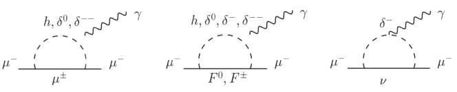
In Fig. 1 we show the Feynman diagrams contributing to the in our model. They are divided into three classes according to the fermions appearing in the loop. Originating from the left, middle and right panel, respectively, the analytical results of generated by our model can be decomposed to
| (47) |
Note that in Fig. 1 the leptons should be understood to carry specifically the muon flavor as .
To write down our analytical results, we first define the following expressions as the reduced form of loop functions (see [57] for a more complete list).
-
•
In calculating from the left panel of Fig. 1 which satisfies , we define
(48) -
•
In calculating from the middle panel of Fig. 1 which satisfies , we define
(49) -
•
In calculating from the right panel of Fig. 1 which satisfies , we define
(50)
The explicit form of originating from the left panel of Fig. 1 is
| (51) |
Note that we have subtracted the SM Higgs contribution from to meet the definition of generated from new physics sector. Moreover, the symmetry factor from the coupling of has been properly considered in as pointed out in Ref. [58].
The explicit form of originating from the middle panel of Fig. 1 is
| (52) |
The explicit form of originating from the right panel of Fig. 1 is
| (53) |
One can clearly see that for each one of the four pieces consisting , the chiral enhancement indicated by or appears in the numerator of the second line. As a result of this enhancement, in Eq. (47) turns out to play the absolutely dominant role compared to and , i.e.
| (54) |
Furthermore, for the different contributions to in Eq. (III.1) , we find that and contribute the dominant and sub-dominant part, respectively.
To simplify our analytical results and highlight the chiral enhancement, we utilize the small mixing condition discussed in Section II.2 and II.3 and extract the most relevant terms in Eq. (III.1) as follows
| (55) |
Considering and we can have the following simple expressions
| (56) |
Based on our calculation we can also reproduce the results of models including only one scalar triplet or one fermion triplet corresponding to Type-II and Type-III seesaw models, respectively. More details can be found in Appendix A.
III.2 Numerical results
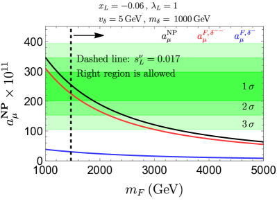
In Fig. 2 we show the new physics contribution predicted by our model in Eq. (47) aiming at interpreting the current deviation of between the experimental measurement and the SM prediction with green color of dark, medium and light opacity indicating the ranges of . Solid black lines denote in Eq. (III.1) which numerically satisfies according to Eq. (III.1). Solid red and blue lines correspond to and in Eq. (III.1) which are the dominant and sub-dominant parts of .
In the left panel of Fig. 2 we impose the scheme described in Eq. (• ‣ II.3) as input parameters. We take as benchmark point and it can be seen that predicted by our model can easily cover the central region of with . In more details, () indicated by red (blue) line contribute about () to the total in the mass range of shown in Fig. 2. Note that according to Eq. (45), only region of is allowed for to satisfy , i.e. the constraints on SM muon neutrino mixing with heavy neutral lepton as discussed in [37]. We can also see that the decoupling behavior of with increasing is clearly manifested. This can be expected from Eq. (• ‣ II.3) since fixed Yukawa couplings with larger would yield smaller mixings and smaller loop function values. More specifically, in the heavy region of we can have the following trending behavior of Eq. (56) after utilizing the approximated form of loop functions in Eq. (• ‣ III.1)
| (57) |
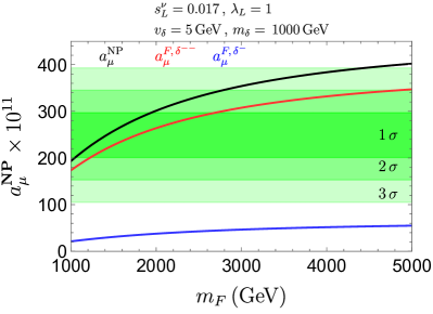
which can be easily seen to decrease with a certain chosen value of and increasing . In the right panel of Fig. 2 we impose the scheme described in Eq. (• ‣ II.3) as input parameters and take as benchmark point. Aside from the observation that can cover the central region of with in this parameter setup, noticeable chiral enhancement is manifested by enhanced when increases.
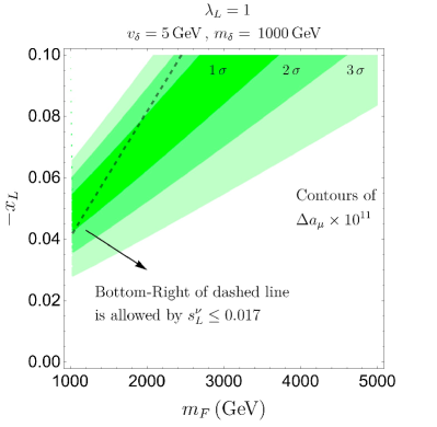
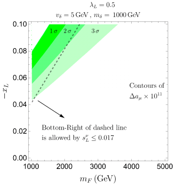
In Fig. 3 we show on the plane of versus in which the left (right) panel has (). The green color of dark, medium and light opacity indicate the ranges of . This figure can be view as the extended illustration of the left panel of Fig. 2 by making to vary. The dashed line denotes with respect to which the bottom-right region is allowed. We can see that in the left panel, the region with and can generate on the edge of region of . In the right panel with , however, the same parameter space with can only generate on the edge of region and thus has little capability of explaining .
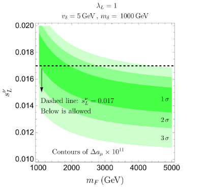
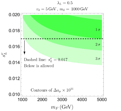
In Fig. 4 we show on the plane of versus in which the left (right) panel has (). This figure can be view as the extended illustration of the right panel of Fig. 2 by making to vary. The dashed line is with respect to which the region below is allowed. We can see that in the left panel, the region with and can generate within the range of . Region with smaller value of would require heavier and thus more significant chiral enhancement to achieve the same level of . The right panel, however, can only generate on the edge of range of with quite heavy fermion mass with . We also checked that all Yukawa couplings in our model satisfy the requirement of perturbativity on the shown range of Fig. 4 which can be easily seen through Eq. (• ‣ II.3).
III.3 Phenomenological discussions
In this section we briefly discuss the phenomenological aspects of our model. Note that the scalar triplet and VLL triplet have been scrutinized in neutrino mass generation mechanisms as Type-II [26, 27, 28, 29, 30, 31] and Type-III [32, 33] seesaw models, respectively. However, in this work we only concentrate on the physics of and do not require our model to produce the experimentally suggested texture of neutrino mass matrix. Instead, we require our model parameters to ensure the theoretically predicted neutrino mass to be negligibly small and close to zero. Aside from the neutrino physics, recently it has been found that the Type-II seesaw model can also address the problem of baryon asymmetry of the universe (see e.g. [59, 60, 61, 62]).
For the new physics leptons , Eq. (39) indicates that the VLL triplet masses are almost degenerate. Originating from the electroweak gauge interactions, can be singly or pairly produced. The main decay channels of the VLL triplet are and . If the mass spectrum satisfies which is assumed in the analysis of this work, there are additional decay channels , . Similarly, for the new physics scalars , Eq. (33) indicates that the scalar triplet mass are also nearly degenerate. The scalar triplet can be pairly or singly produced through the -channel mediation of SM gauge bosons . The fermionic decay channels of the scalar triplet to SM leptons include , , and . The bosonic decay channels of the scalar triplet to SM bosons include , , and , of which the partial decay widths are proportional to . If the mass spectrum satisfies , there are additional decay channels , , and . Detailed collider analysis is beyond the scope of this paper, and recent discussions on the prospects of searches for scalar triplet around TeV at future high luminosity LHC and 100 TeV collider can be found in [63] and [41], respectively.
IV Conclusions
In this work, we investigated the muon anomalous dipole moment in a model that extends the SM with a scalar triplet and a vector-like lepton triplet. We identify an important ingredient overlooked in previous studies, i.e. the Yukawa interaction involving the SM Higgs doublet and the newly introduced lepton triplet. This interaction is a four-dimensional operator and thus can naturally exist. We show that this Yukawa interaction can not only induce mass mixing between leptons in the SM and the new physics sector, but also provide an additional source of chiral flipping to . We find that there is still viable parameter space in this model to explain , which is different from the observation reported in the existing literature. More specifically, while being consistent with the current data of neutrino mass, precision electroweak measurements and the perturbativity of couplings, our model can provide new physics contribution to cover the central region of with new scalar and fermion mass as low as around TeV. This mass scale is allowed by the current collider searches for doubly charged scalars and vector-like leptons, and they can be tested at future high energy and/or high luminosity colliders.
Acknowledgements.
This work was supported by National Key R&D Program of China under grant Nos. 2023YFA1606100. CH is supported by the Sun Yat-Sen University Science Foundation. SH is supported by the research start-up fund of Taiyuan University of Technology. SH would also like to acknowledge the hospitality of Center for High Energy Physics, Peking University, where he spent three months as a visitor. PW acknowledges support from Natural Science Foundation of Jiangsu Province (Grant No. BK20210201), Fundamental Research Funds for the Central Universities, Excellent Scholar Project of Southeast University (Class A), and the Big Data Computing Center of Southeast University.Appendix A Reproduced results in models including only one scalar triplet or one VLL triplet
If keeping only the scalar triplet or the VLL triplet in Section III.1 by turning off relevant interactions, we can reproduce the analytical results of predicted in Type-II and Type-III seesaw models.
- •
-
•
By taking , the vanishes automatically and we would reproduce the results in Type-III seesaw model as follows
(59)
References
- [1] Muon g-2 collaboration, G. W. Bennett et al., Final Report of the Muon E821 Anomalous Magnetic Moment Measurement at BNL, Phys. Rev. D 73 (2006) 072003 [hep-ex/0602035].
- [2] F. Jegerlehner and A. Nyffeler, The Muon g-2, Phys. Rept. 477 (2009) 1 [0902.3360].
- [3] F. Jegerlehner, The Anomalous Magnetic Moment of the Muon, vol. 274. Springer, Cham, 2017, 10.1007/978-3-319-63577-4.
- [4] T. Aoyama et al., The anomalous magnetic moment of the muon in the Standard Model, Phys. Rept. 887 (2020) 1 [2006.04822].
- [5] Muon g-2 collaboration, B. Abi et al., Measurement of the Positive Muon Anomalous Magnetic Moment to 0.46 ppm, Phys. Rev. Lett. 126 (2021) 141801 [2104.03281].
- [6] P. Cox, C. Han and T. T. Yanagida, Muon g-2 and coannihilating dark matter in the minimal supersymmetric standard model, Phys. Rev. D 104 (2021) 075035 [2104.03290].
- [7] P. Cox, C. Han, T. T. Yanagida and N. Yokozaki, Gaugino mediation scenarios for muon and dark matter, JHEP 08 (2019) 097 [1811.12699].
- [8] C. Han, M. L. López-Ibáñez, A. Melis, O. Vives, L. Wu and J. M. Yang, LFV and (g-2) in non-universal SUSY models with light higgsinos, JHEP 05 (2020) 102 [2003.06187].
- [9] C. Han, Muon g-2 and CP violation in MSSM, 2104.03292.
- [10] Muon g-2 collaboration, G. Venanzoni, New results from the Muon g-2 Experiment, PoS EPS-HEP2023 (2024) 037 [2311.08282].
- [11] S. Kuberski, M. Cè, G. von Hippel, H. B. Meyer, K. Ottnad, A. Risch et al., Hadronic vacuum polarization in the muon g 2: the short-distance contribution from lattice QCD, JHEP 03 (2024) 172 [2401.11895].
- [12] A. Boccaletti et al., High precision calculation of the hadronic vacuum polarisation contribution to the muon anomaly, 2407.10913.
- [13] A. Freitas, J. Lykken, S. Kell and S. Westhoff, Testing the Muon g-2 Anomaly at the LHC, JHEP 05 (2014) 145 [1402.7065].
- [14] K. Kowalska and E. M. Sessolo, Expectations for the muon g-2 in simplified models with dark matter, JHEP 09 (2017) 112 [1707.00753].
- [15] L. Calibbi, R. Ziegler and J. Zupan, Minimal models for dark matter and the muon g2 anomaly, JHEP 07 (2018) 046 [1804.00009].
- [16] P. Athron, C. Balázs, D. H. J. Jacob, W. Kotlarski, D. Stöckinger and H. Stöckinger-Kim, New physics explanations of aμ in light of the FNAL muon g 2 measurement, JHEP 09 (2021) 080 [2104.03691].
- [17] A. Cherchiglia, D. Stöckinger and H. Stöckinger-Kim, Muon g-2 in the 2HDM: maximum results and detailed phenomenology, Phys. Rev. D 98 (2018) 035001 [1711.11567].
- [18] M. Pospelov, Secluded U(1) below the weak scale, Phys. Rev. D 80 (2009) 095002 [0811.1030].
- [19] W. Chao, The Muon Magnetic Moment in the TeV Scale Seesaw Models, 0806.0889.
- [20] C. Biggio, The Contribution of fermionic seesaws to the anomalous magnetic moment of leptons, Phys. Lett. B 668 (2008) 378 [0806.2558].
- [21] T. Moroi, The Muon anomalous magnetic dipole moment in the minimal supersymmetric standard model, Phys. Rev. D 53 (1996) 6565 [hep-ph/9512396].
- [22] D. Stockinger, The Muon Magnetic Moment and Supersymmetry, J. Phys. G 34 (2007) R45 [hep-ph/0609168].
- [23] S.-P. He, Leptoquark and vectorlike quark extended models as the explanation of the muon anomaly, Phys. Rev. D 105 (2022) 035017 [2112.13490].
- [24] S.-P. He, Leptoquark and vector-like quark extended model for simultaneous explanation of W boson mass and muon g–2 anomalies*, Chin. Phys. C 47 (2023) 043102 [2205.02088].
- [25] S.-P. He, Scalar leptoquark and vector-like quark extended models as the explanation of the muon g–2 anomaly: bottom partner chiral enhancement case*, Chin. Phys. C 47 (2023) 073101 [2211.08062].
- [26] M. Magg and C. Wetterich, Neutrino Mass Problem and Gauge Hierarchy, Phys. Lett. B94 (1980) 61.
- [27] J. Schechter and J. W. F. Valle, Neutrino Masses in Theories, Phys. Rev. D22 (1980) 2227.
- [28] C. Wetterich, Neutrino Masses and the Scale of B-L Violation, Nucl. Phys. B187 (1981) 343.
- [29] G. Lazarides, Q. Shafi and C. Wetterich, Proton Lifetime and Fermion Masses in an SO(10) Model, Nucl. Phys. B181 (1981) 287.
- [30] R. N. Mohapatra and G. Senjanovic, Neutrino Masses and Mixings in Gauge Models with Spontaneous Parity Violation, Phys. Rev. D23 (1981) 165.
- [31] T. P. Cheng and L.-F. Li, Neutrino Masses, Mixings and Oscillations in Models of Electroweak Interactions, Phys. Rev. D22 (1980) 2860.
- [32] R. Foot, H. Lew, X. G. He and G. C. Joshi, Seesaw Neutrino Masses Induced by a Triplet of Leptons, Z. Phys. C 44 (1989) 441.
- [33] E. Ma and D. P. Roy, Heavy triplet leptons and new gauge boson, Nucl. Phys. B 644 (2002) 290 [hep-ph/0206150].
- [34] A. Arhrib, R. Benbrik, M. Chabab, G. Moultaka, M. C. Peyranere, L. Rahili et al., The Higgs Potential in the Type II Seesaw Model, Phys. Rev. D 84 (2011) 095005 [1105.1925].
- [35] M. Sajjad Athar et al., Status and perspectives of neutrino physics, Prog. Part. Nucl. Phys. 124 (2022) 103947 [2111.07586].
- [36] Particle Data Group collaboration, R. L. Workman et al., Review of Particle Physics, PTEP 2022 (2022) 083C01.
- [37] F. del Aguila, J. de Blas and M. Perez-Victoria, Effects of new leptons in Electroweak Precision Data, Phys. Rev. D 78 (2008) 013010 [0803.4008].
- [38] A. Abada, C. Biggio, F. Bonnet, M. B. Gavela and T. Hambye, mu — e gamma and tau — l gamma decays in the fermion triplet seesaw model, Phys. Rev. D 78 (2008) 033007 [0803.0481].
- [39] CMS collaboration, A. M. Sirunyan et al., Search for vector-like leptons in multilepton final states in proton-proton collisions at = 13 TeV, Phys. Rev. D 100 (2019) 052003 [1905.10853].
- [40] ATLAS collaboration, G. Aad et al., Search for type-III seesaw heavy leptons in leptonic final states in pp collisions at with the ATLAS detector, Eur. Phys. J. C 82 (2022) 988 [2202.02039].
- [41] Y. Du, A. Dunbrack, M. J. Ramsey-Musolf and J.-H. Yu, Type-II Seesaw Scalar Triplet Model at a 100 TeV Collider: Discovery and Higgs Portal Coupling Determination, JHEP 01 (2019) 101 [1810.09450].
- [42] J. F. Gunion, H. E. Haber, G. L. Kane and S. Dawson, The Higgs Hunter’s Guide, vol. 80. 2000, 10.1201/9780429496448.
- [43] M. Aoki, S. Kanemura, M. Kikuchi and K. Yagyu, Radiative corrections to the Higgs boson couplings in the triplet model, Phys. Rev. D 87 (2013) 015012 [1211.6029].
- [44] ATLAS collaboration, G. Aad et al., Observation of a new particle in the search for the Standard Model Higgs boson with the ATLAS detector at the LHC, Phys. Lett. B 716 (2012) 1 [1207.7214].
- [45] CMS collaboration, S. Chatrchyan et al., Observation of a New Boson at a Mass of 125 GeV with the CMS Experiment at the LHC, Phys. Lett. B 716 (2012) 30 [1207.7235].
- [46] P. S. B. Dev, C. M. Vila and W. Rodejohann, Naturalness in testable type II seesaw scenarios, Nucl. Phys. B 921 (2017) 436 [1703.00828].
- [47] CMS collaboration, A search for doubly-charged Higgs boson production in three and four lepton final states at , .
- [48] ATLAS collaboration, G. Aad et al., Search for doubly charged Higgs boson production in multi-lepton final states using 139 fb-1 of proton–proton collisions at = 13 TeV with the ATLAS detector, Eur. Phys. J. C 83 (2023) 605 [2211.07505].
- [49] ATLAS collaboration, Combined measurements of Higgs boson production and decay using up to fb-1 of proton-proton collision data at TeV collected with the ATLAS experiment, (2021) .
- [50] CMS collaboration, Combined Higgs boson production and decay measurements with up to 137 fb-1 of proton-proton collision data at = 13 TeV, (2020) .
- [51] N. D. Christensen and C. Duhr, FeynRules - Feynman rules made easy, Comput. Phys. Commun. 180 (2009) 1614 [0806.4194].
- [52] A. Alloul, N. D. Christensen, C. Degrande, C. Duhr and B. Fuks, FeynRules 2.0 - A complete toolbox for tree-level phenomenology, Comput. Phys. Commun. 185 (2014) 2250 [1310.1921].
- [53] T. Hahn, Generating Feynman diagrams and amplitudes with FeynArts 3, Comput. Phys. Commun. 140 (2001) 418 [hep-ph/0012260].
- [54] T. Hahn, S. Paßehr and C. Schappacher, FormCalc 9 and Extensions, PoS LL2016 (2016) 068 [1604.04611].
- [55] H. H. Patel, Package-X: A Mathematica package for the analytic calculation of one-loop integrals, Comput. Phys. Commun. 197 (2015) 276 [1503.01469].
- [56] H. H. Patel, Package-X 2.0: A Mathematica package for the analytic calculation of one-loop integrals, Comput. Phys. Commun. 218 (2017) 66 [1612.00009].
- [57] S.-P. He, Handbook of the analytic and expansion formulae for the muon anomaly, 2308.07133.
- [58] F. S. Queiroz and W. Shepherd, New Physics Contributions to the Muon Anomalous Magnetic Moment: A Numerical Code, Phys. Rev. D 89 (2014) 095024 [1403.2309].
- [59] N. D. Barrie, C. Han and H. Murayama, Affleck-Dine Leptogenesis from Higgs Inflation, Phys. Rev. Lett. 128 (2022) 141801 [2106.03381].
- [60] N. D. Barrie, C. Han and H. Murayama, Type II Seesaw leptogenesis, JHEP 05 (2022) 160 [2204.08202].
- [61] C. Han, S. Huang and Z. Lei, Vacuum stability of the type II seesaw leptogenesis from inflation, Phys. Rev. D 107 (2023) 015021 [2208.11336].
- [62] C. Han, Z. Lei and J. M. Yang, Type-II Seesaw Leptogenesis along the Ridge, 2312.01718.
- [63] P. D. Bolton, J. Kriewald, M. Nemevšek, F. Nesti and J. C. Vasquez, On Lepton Number Violation in the Type II Seesaw, 2408.00833.
- [64] M. Lindner, M. Platscher and F. S. Queiroz, A Call for New Physics : The Muon Anomalous Magnetic Moment and Lepton Flavor Violation, Phys. Rept. 731 (2018) 1 [1610.06587].