Measuring using DESI Legacy Imaging Surveys Emission-Line Galaxies and Planck CMB Lensing, and the Impact of Dust on Parameter Inference
Abstract
Measuring the growth of structure is a powerful probe for studying the dark sector, especially in light of the tension between primary CMB anisotropy and low-redshift surveys. This paper provides a new measurement of the amplitude of the matter power spectrum, , using galaxy-galaxy and galaxy-CMB lensing power spectra of Dark Energy Spectroscopic Instrument Legacy Imaging Surveys Emission-Line Galaxies and the Planck 2018 CMB lensing map. We create an ELG catalog composed of million galaxies and with a purity of , covering a redshift range , with . We implement several novel systematic corrections, such as jointly modeling the contribution of imaging systematics and photometric redshift uncertainties to the covariance matrix. We also study the impacts of various dust maps on cosmological parameter inference. We measure the cross-power spectra over with a signal-to-background ratio of up to . We find that the choice of dust maps to account for imaging systematics in estimating the ELG overdensity field has a significant impact on the final estimated values of and , with far-infrared emission-based dust maps preferring to be as low as , and stellar-reddening-based dust maps preferring as high as . The highest preferred value is at tension with the Planck primary anisotropy results. These findings indicate a need for tomographic analyses at high redshifts and joint modeling of systematics.
1 Introduction
The discovery of the accelerated expansion of the Universe [1, 2] with the help of Type Ia supernovae, the cosmic microwave background (CMB) acoustic peaks [3, 4], and the Baryonic Acoustic Oscillation (BAO) in the large-scale structure [5] established dark energy as the leading explanation for the observed cosmic acceleration. These cosmology experiments identify the existence of dark energy by measuring the Hubble constant, .
The negative pressure of dark energy inhibits the growth of large-scale structures, countering the force of gravitation [6], which has led to the measurement of structure growth as a power probe of dark energy complimentary to that from distance measurements. Suppression of the growth of large-scale structure is best measured with experiments that focus on weak gravitational lensing (galaxy-galaxy, cosmic shear, or CMB lensing), galaxy cluster counting, and redshift space distortions [7]. These experiments essentially measure the combination of the amplitude of the matter power spectrum, , and the cosmic matter density, , by using matter tracers such as lensing fields, galaxy clusters, or spectroscopic surveys.
These probes and the individual experiments have shown remarkable agreement with the CDM paradigm. However, we have seen statistically significant disagreements between cosmological parameters inferred from CMB and late-time experiments in recent years. For example, the inferred measurement of from CMB experiments such as Planck [8] and the Atacama Cosmology Telescope (ACT) [9] are at about odds with Type Ia Supernovae probes [10]. Similarly, the inferred measurement of from CMB experiments such as Planck and ACT are at about odds with late-Universe probes such as weak lensing [11, 12, 13, 14], spectroscopic galaxy clustering [15], redshift space distortions [16] and galaxy cluster counting [17, 18].
The presence of these so-called tensions between the early Universe and the late Universe is tantalizing; it may indicate the existence of new unknown physics, such as modification of gravity or dark energy (a detailed discussion can be found at [19]). However, a more down-to-earth explanation could be that previously unquantified systematic uncertainties induce these tensions. Cross-correlation of matter tracers with very different systematic properties could address this explanation [6]. The aforementioned weak lensing experiments often take a approach where they measure the auto-correlation of individual tracers and also their cross-correlation to mitigate the effect of systematics and to break parameter degeneracy. More recently, such techniques have also been used to combine galaxy clustering measurements with CMB lensing [20, 21, 22, 23, 24, 25]; some of these studies have shown mild tension in the parameter space when compared to Planck. The bulk of the growth of structure studies has been conducted with tracers at ; thus, the tension we observe is between the and Universe. This fact leads to the question of whether the answer lies in the intermediate redshift () Universe because if CDM is assumed to be accurate, then it is around when the dark energy density, became the same order of magnitude as the matter density, , for the first time in the cosmic history. Thus, there may be observable effects during this turnover period.
Interestingly, some recent studies that use the Atacama Cosmology Telescope (ACT) data [22, 26] do not find this tension. Thus, it has become even more critical to understand the physics of the Universe to ascertain whether the deviations seen by earlier works are due to cosmology, astrophysics or systematics.
The Dark Energy Spectroscopic Instrument (DESI) Legacy Imaging Surveys [27] and the ongoing DESI spectroscopic survey111”DESI Collaboration Key Paper”. Part of Key Project 1, convener: Paul Martini [28] have provided a new window to exploring the epoch of our Universe using galaxy clustering. DESI is a highly multiplexed spectroscopic surveyor that can obtain simultaneous spectra of almost objects over a field [29, 30, 31], is currently conducting a five-year survey of about a third of the sky. This campaign will obtain spectra for approximately million galaxies and quasars [32].
Both the Legacy Imaging Surveys and the DESI spectroscopic survey use emission-line galaxies (ELGs) as matter tracers to probe the Universe with the highest number density and sky coverage to-date. As the cosmic star formation rate peaks around [33], so does the number density of these star-forming ELGs. Thus, ELGs provide a unique window to the intermediate redshift Universe. Ongoing and future galaxy surveys such as Euclid, Roman, and the Rubin Observatory will use ELG-like galaxies to push beyond . The Legacy Surveys is the photometric catalog for DESI; it covers of the sky and contains million objects deemed as ELGs, thus making it the largest photometric ELG catalog to date.
In this paper, for the first time, we use the ELG targets from the Legacy Surveys and cross-correlate them with the Planck CMB lensing map to constrain the growth of structure by measuring the ELG auto- and ELG-CMB lensing cross-power spectra. Given the size of the Legacy Surveys catalog, this is the most extensive analysis of ELGs as a cosmological tracer in a cross-correlation study. Additionally, we thoroughly analyze various systematics, especially how the choice of dust maps to correct foreground systematics affects cosmological parameter inference.
We structure this paper as follows: Section 2 describes the Legacy Surveys, DESI Survey Validation, and the Planck CMB lensing datasets. Section 3 discusses how we selected our ELG sample and estimated the redshift distribution. In Section 4 we discuss the various modeling aspects of our analysis. Section 5 discusses our choices for the likelihood inference framework as well as how we estimated the associated covariance matrix. In Section 6, we showcase the validation of our analysis pipeline. Section 7 presents the key findings of our paper, and in Section 8 contextualizes the results. Finally in Section 9 we summarize the results.
2 Data
The overlapping footprint of the Planck CMB lensing and the Legacy Surveys maps is about of the entire sky, allowing us to take relatively large modes into account for our analysis, compared to previous studies.
For this analysis, we select galaxies that make it through the DESI Survey Validation 3 (SV3) color cuts in the g - r versus r - z parameter space (DESI-like ELGs). Here g, r, and z refer to green at nm, red at nm, and extended infrared at nm. DESI-like ELGs are a natural choice for this analysis because DESI has already made many observations during its Survey Validation phase and internally released reduced spectra and spectroscopic redshifts of about ELGs. These spectroscopic redshifts are invaluable in calibrating the photometric redshift distribution that we use in our analysis and for deciding which ELGs belong to which tomographic bins.
In the following sections, we briefly describe the three key datasets for our analysis – the Planck CMB lensing map in Section 2.1, the Legacy Surveys DR9 catalog in Section 2.2 and the DESI SV3 fuji catalog in Section 2.3.
2.1 Planck CMB lensing map
The Planck collaboration published the PR3 CMB lensing map in 2018 [34]. The CMB lensing map traces the distortion of the CMB photons along the line of sight as they encounter the gravitational potential of masses. Depending on the geometry between the surface of the last scattering and the observer, the gravitational potential can deflect the CMB photons, distorting the observed temperature and polarization anisotropies. By carefully studying the statistical patterns of these distortions, one can reconstruct the intervening projected gravitational potential kernel, which tells us the projected distribution of mass between us and the surface of the last scattering. Hence, the CMB lensing map traces the matter distribution exactly and is an unbiased tracer of matter density distribution in the Universe.
For this analysis, we use the minimum-variance lensing estimates from the SMICA DX12 CMB maps222https://wiki.cosmos.esa.int/planck-legacy-archive/index.php/Lensing. We specifically use the com_lensing_4096_r3.00 dataset that provides the baseline lensing convergence estimates in spherical harmonics basis, up to . The observed lensing convergences are measured using temperature and polarization maps. In addition, the dataset contains the Planck convergence reconstruction approximate noise, , and the survey mask.
Note that the Planck CMB lensing reconstruction is noise-dominated at almost every scale, especially at high-. It becomes especially problematic when using a pseudo- estimator because the finite survey size causes mode-mode coupling and the noise from high- can leak into low- scales of interest (see Section 4). Hence, we first process the data with a low-pass filter. This function allows us to smoothly truncate the power to above a specific scale; we set and to be and respectively as we constrain our analysis in the range . The low-pass-filtered is given by:
We then rotate the filtered and the Planck mask from the Galactic coordinate basis to the Equatorial coordinate basis since we perform our analysis in Equatorial coordinates. In the new basis, we apodize the provided mask to allow it to go smoothly to in real space. We specifically use the “C2” apodization scheme from the package NaMaster [35] with an apodization scale of deg which is optimal for the size of holes in the Planck mask [23].
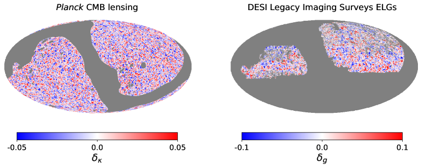
The final CMB lensing map is in Figure 1, where we have smoothed the map with a Gaussian for visualization.
2.2 Legacy Surveys DR9 catalogue
The Legacy Surveys333https://www.legacysurvey.org/ is an inference model catalog of three different surveys – the Dark Energy Camera Legacy Survey (DECaLS), the Beijing-Arizona Sky Survey (BASS) and the Mayall -band Legacy Survey – that jointly cover about deg2 of the sky visible from the Northern hemisphere in -, - and -bands as well as four WISE infrared bands [27]. The main motivation for the Legacy Surveys was to serve as the photometric input catalog of the DESI experiment; to achieve and maximize its scientific goals, DESI requires reliable photometry with sufficient depth to select target objects a priori. The average galaxy depth for the -, - and -bands are , and AB magnitudes respectively.
Because of its exact footprint overlap with the DESI Survey Validation, the DESI main survey, and the wide area coverage, the Legacy Surveys serve as the ideal photometric dataset for our cross-correlation analysis. Specifically, since the same cuts on the color and magnitude spaces that have been applied to select the DESI Survey Validation ELG targets can be applied to the full Legacy Surveys dataset, we can ensure that we are selecting galaxy populations with similar properties. As a result, we can robustly rely on using the spectroscopic redshift distribution, , as the redshift calibrator for our photometric sample and make tomographic bin assignments.
The ninth data release444https://www.legacysurvey.org/dr9/description/ of the Legacy Surveys (hereafter DR9) is the final data release of the Legacy Surveys, which brings all three separate surveys under one reduction pipeline and produces uniform photometry across the three surveys, making it a robust galaxy catalog to probe large-scale modes. The DR9 catalog contains about million objects photometrically deemed ELGs.
2.3 DESI SV3 fuji catalogue
The fuji spectroscopic catalog is an internal data release within the DESI collaboration that contains all the commissioning and survey validation data. The goal of DESI is to determine the nature of dark energy by measuring the expansion of the Universe [36]. The sheer scale of the DESI experiment requires an extensive spectroscopic reduction pipeline [37], a template-fitting pipeline to derive classifications and redshifts for each targeted source [38], a pipeline to tile the survey and to plan and optimize observations as the campaign progresses [39], a pipeline to select targets for spectroscopic follow-up [40], and Maskbit to generate ”clean” photometry [41].
The primary motivation of the survey validation (SV) phase555“DESI Collaboration Key Paper”. Part of Key Project 1, conveners: Kyle Dawson and Christophe Yèche [42] of the project was to ensure that the DESI instrument met its spectroscopic performance goals, the requirements as a Stage-IV dark energy experiment, fine-tune the target selection algorithms.
The fuji SV3 catalog contains objects that were photometrically deemed as ELGs, covering about deg2 of the sky. After rejecting objects whose observed spectra were flagged by the spectral pipeline, we obtained a total of ELGs, giving the SV3 sample a number density of about per deg2. Additionally, compared to the ongoing DESI survey, the SV dataset has much deeper spectroscopy, and the ELGs were given equal priority in fiber assignment, making it a suitable dataset for ELG redshift distribution calibration. All the fuji ELGs are included in the Early DESI Data Release666“DESI Collaboration Key Paper”. Part of Key Project 1, conveners: Anthony Kremin and Stephen Bailey [43].
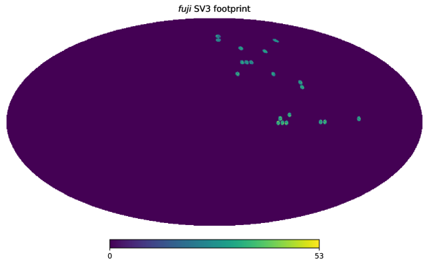
Additionally, the SV3 dataset is ideal for dealing with the issue of sample variance. Sample variance in this context refers to the problem of obtaining spectroscopic to photometric redshift calibration from a small patch of the sky. Suppose the galaxy population living in a small patch of the sky does not represent the galaxy population at large. In that case, if the patch traces an underdense or an overdense region in the large-scale structures, the redshift calibration we obtain will be biased. However, as shown in Figure 2, the SV3 footprint is spread out in different small patches of the sky, reducing the impact of sample variance.
3 Preparation of ELG sample
We select the final ELG sample based on photometric features in the DR9 catalog. We initially take the DESI ELG target selection function [44, 45, 46] and apply further selection cuts to increase the purity of the final ELG sample. Our selection uses features – flux_g, flux_r and flux_z corresponding to the model flux in the , and bands, and colors and fiberflux_g, fiberflux_r and fiberflux_z corresponding to the expected fiber magnitude of the target sources assuming a diameter fiber with a Gaussian seeing. The fluxes and the fiber fluxes are converted to magnitudes and corrected for Milky Way transmission using the features mw_transmission_g, mw_transmission_r and mw_transmission_z. We refer to the fiber magnitudes as , , and , respectively. In the following sections, we discuss the various choices we make in preparing the final sample.
3.1 Selection of galaxy sample based on photometric and spectroscopic properties
As we use the fuji spectroscopic sample to select ELGs from the DR9 catalog, we run several quality checks on the fuji catalog to define what magnitude and color cuts will define our final sample. These quality checks are necessary to understand whether there are contaminants such as stars, QSOs, and low-redshift interlopers, whose photometric properties are similar to ELGs in the desired redshift range. How these contaminants cluster in the color-magnitude-fiber magnitude space is essential to removing them from our final sample. In addition, these quality checks also help us determine which parts of the data have reliable spectroscopic redshifts to ensure accurate photometric redshift calibration.
Our quality checks took two forms: 1) for objects based on photometric properties such as the targets’ colors, magnitudes or shapes, we apply the same quality cuts on the photometric sample; 2) for objects whose quality cuts depend on spectroscopic properties such as the signal-to-noise of the [O ii] doublet lines, we look for how galaxies with undesirable properties cluster in the color magnitude space. We train a Random Forest classifier [47] on these clustering properties to delineate where the undesirable galaxies live in this -dimensional space and use the Random Forest on the photometric sample to remove galaxies with similar properties.
When processing the fuji catalog, we remove all targets that have been flagged by the DESI spectral pipeline. These quality checks are listed below:
-
•
We select targets with good photometry. Targets with bad photometry are masked in the column photsys.
-
•
We select targets that the pipeline considers to have reliable co-added spectra for spectroscopic redshift measurement; we accomplish this task by selecting targets whose coadd_fiberstatus .
With the above selection applied, a clean catalog is obtained in which further cuts are made on the photometric properties:
-
•
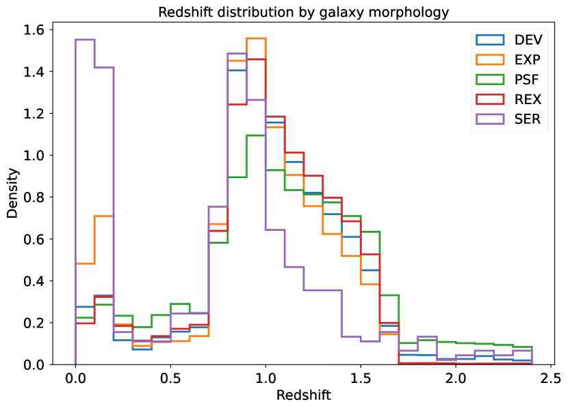
We remove targets whose morphology corresponds to the Sersic profile according to the DR9 catalog pipeline; we accomplish this task by selecting targets with morphtype ser. We remove Sersic profile targets because when we look at the spectroscopic redshift distribution of the targets as a function of their morphology, we find that more than half of the Sersic profile targets are low-redshift interlopers (Figure 3). In addition, the Sersic profile targets form only of the overall catalog. Hence, removing them does not affect the overall number density by any discernible amount.
-
•
We remove targets with shape_r arcsec. shape_r refers to the half-light radius of galaxies with extended morphologies. We find that targets with larger half-light radii make up only of the total sample. Therefore, calibration concerning these galaxies will be more prone to shot noise.
-
•
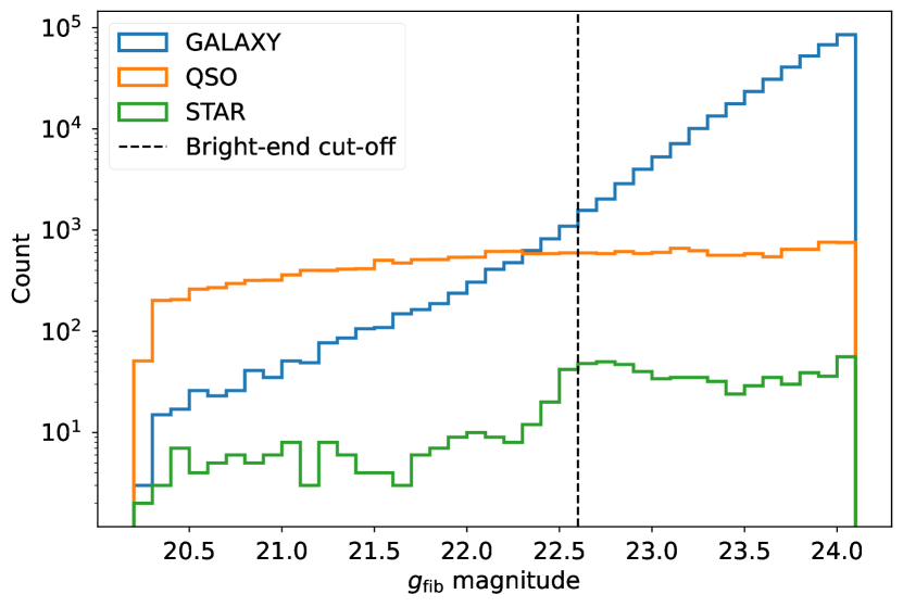
We apply a fiber magnitude bright end cut of because below this threshold, a large fraction of ELG targets are deemed as QSOs by the DESI pipeline (Figure 4). Specifically, the fraction of QSO contaminants is and below and above the threshold, respectively. Since the QSOs may have a different linear bias than the ELGs, we apply this cut to obtain a purer sample. As a result, we discard of the fuji sample.
-
•
We look at the histograms of the different photometric features and apply cuts to select the most sampled region in the color-magnitude-fiber magnitude space with the following: , , , , , and .
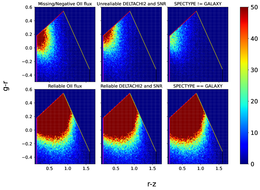
Next, we look at how the targets that the spectroscopic pipeline flags as contaminants cluster in the color-magnitude-fiber magnitude space. There are three sources of contamination – (i) ELG targets with spectroscopic redshift because these do not fall into our redshift range sample, (ii) ELG targets that the spectroscopic pipeline flags as not galaxies, (iii) targets present in fuji whose spectroscopic properties make them unreliable for spectroscopic redshift measurements.
To isolate these contaminants from the good targets, we train a Random Forest Classifier that draws decision boundaries in the color-magnitude-fiber magnitude space based on labels for each ELG target in the fuji sample. We denote ELGs that have spectroscopic redshifts in the range as Label , low-redshift interlopers belonging to category (i) as label and contaminants belonging to categories (ii) and (iii) as label . Thus, with each target assigned a label in the fuji catalog, the Random Forest Classifier learns to identify which parts of the feature space belong to our desired category, i.e., , and which ones belong to the ones we do not want in our sample, i.e., and .
We identify these contaminants as follows:
-
•
We look at the column spectype in the fuji catalogue. This column indicates whether the DESI pipeline deemed the target galaxy, a QSO, or a star. We select targets that meet the requirement spectype galaxy. We find that and of the ELG targets in fuji are QSOs and stars, respectively. These latter contaminants are assigned as Label .
-
•
We consider any ELG targets with no or negative [O ii] flux as bad because [O ii] doublet is the key signature the DESI pipeline uses to measure spectroscopic redshift. These targets are also assigned as Label .
-
•
Reference [44] showed that there is a relationship between the reliability of spectroscopic redshift measured by the DESI pipeline and the two spectroscopic features, foii_snr and deltachi2. foii_snr refers to the signal-to-noise of the measured [O ii] flux and deltachi2 refers to the difference between the best-fit template and the second-best-fit template. Based on visual inspection of ELGs in the SV sample, Reference [44] shows that ELGs that have reliable spectroscopic redshift obey the following relationship: . We apply this same criterion to the fuji ELGs and assign Label to any targets that fail this criterion.
-
•
Finally, we look at the spectroscopic redshifts of the galaxies that pass the three criteria mentioned above. Any targets with are assigned the Label , and the rest are assigned the Label .
These contaminants cluster in a specific way on the color-magnitude-fiber magnitude space. We show this clustering on the versus space as an example in Figure 5, where we show D histograms of these contaminants.
3.2 Random Forest Classifier training
Once all the targets in the fuji catalog are assigned labels, we train a random forest classifier to determine which regions in the color-magnitude-fiber magnitude space are unreliable for spectroscopic redshift calibration. We make a split to prepare the training and test sets.
We make this split by fields rather than by randomly selecting of the data as the training set. Figure 2 shows ELG fields observed in the fuji catalog; we choose fields without replacement as training sets, and the rest of fields are the test sets. We split in this specific way to deal with the so-called sample variance of the calibration set; if a particular field by chance lies on a highly fluctuating region, e.g., a void or a galaxy cluster, then calibrating against it would introduce bias [48]. Hence, the split by fields ensures we are accounting for such variances.
However, with a bin width of , the total number of bins we are estimating is , while the number of independent fields we have is . Thus, to have the number of training sets in the same order of magnitude as the number of histogram parameters, we further divide the ELG fields into equal halves to create a total of fields. As a result, we ultimately use fields for training and for testing. Since the Random Forest Classifier has many hyperparameters, we tune the hyperparameters using the scikit-learn [49] function RandomSearchCV. The tuned hyperparameters are listed in Table 1.
| Hyperparameters | Values |
|---|---|
| class_weight | [0: 0.325, 1: 0.35, 2: 0.325] |
| max_features | sqrt |
| min_samples_leaf | 10 |
| min_samples_split | 10 |
| n_estimators | 20 |
This procedure selects about million ELGs from the parent ELG sample in the Legacy Surveys, yielding an overall ELG number density of about deg-2.
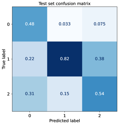
Overall, the training sample is composed of , and of Label , and respectively. The Random Forest Classifier training results are shown in Figure 6; the columns are normalized to reflect what fraction of the Classifier predicted labels are false positives. Compared to the baseline, we have a improvement in identifying label objects. Although the Classifier predicts of the Label objects as Label , we can model these objects into our analysis since we know their spectroscopic redshifts. In contrast, the Classifier predicts of the Label objects as Label objects. We discuss in-depth how we model these objects in Section 3.3.
3.3 Modeling Redshift Distribution of Unknown Galaxies
The confusion matrix plot (Figure 6) shows that the Classifier misclassifies of Label objects as Label objects, i.e., galaxies that the Classifier considers to be in the redshift range , but do not have secured spectroscopic redshift measurements. Thus, while these galaxies contribute to the angular clustering measurements, without knowing their redshifts, it is not easy to assess their contribution to the overall power spectra. Therefore, we develop a model to estimate the redshift distribution of these Label galaxies misclassified as being Label . Note that the integral of the density normalized redshift histogram of the known galaxies and these unknown galaxies should add up to because these two types of galaxies make up all the samples in the defined color-magnitude-fiber magnitude space. Keeping this in mind, we make some assumptions about their distributions:
-
•
We assume that a fraction of these unknown galaxies are ; hence, DESI could not locate any [O ii] doublets to get secured redshift measurements. This assumption is valid because galaxies just above have similar color-magnitude-fiber magnitude properties to those just below the redshift threshold. However, since we do not know what this fraction is, we assign a sampling variable, , between and the failure rate, .
-
•
We further assume that the fraction of objects is in our desired tomographic range, except for stochastic reasons, we could not estimate their redshifts. Thus, we rescale the known redshift bins by that fraction.
-
•
Finally, we assume that the objects fall off exponentially with redshift, meaning that it is more likely that we have ELGs in the bin than in the bin . Our assumption implies that galaxies from a vastly different redshift would have characteristically different color-magnitude-fiber magnitude properties. Since we know the bin values below , and represents the area under the curve for of the redshift distribution, we have a unique exponential decay curve for each of the bootstrapped redshift distributions. We go up to and get the final curves in Figure 7. We derive the functional form of the exponential tail of the redshift distribution in Appendix A.
As an illustrative example, consider a bootstrap run where the Random Forest Classifier misclassified of Label objects as being ; we have to model the redshift distribution of this . First, we uniformly sample a number, . We rescale the known redshift bins by . Afterwards, since we know the value of the last bin, it serves as the first point of the exponential decay curve. The total area under this curve has to be equal to . The first point of the decay curve and the total area under it uniquely define it. Thus, we obtain the redshift distribution of all the galaxies.
This estimation is, of course, inherently noisy due to the assumptions made. However, in the absence of deep spectroscopic samples that we can use to calibrate the misclassified objects, our method is robust enough to handle this problem. We explicitly account for the uncertainty coming from this method in the covariance matrix; we produce correlated Gaussian mocks with these bootstrapped values to estimate the final covariance matrix, following the approach outlined in Reference [50].
3.4 Estimating Redshift Distribution Uncertainty

We use the bootstrap resampling method [51] to estimate the redshift distribution uncertainty. We do this by splitting the fields into two sets of and fields, respectively; these form the basis for the training and the test sets. Then, we resample the indices of the training fields and the test fields with replacements. We use the resampled training fields to train the Random Forest Classifier with the same hyperparameters as Table 1 to estimate the redshift distribution. We do this times shown by the black curves in Figure 7, and the cyan curve represents the photometric redshift distribution based on the training of the Random Forest Classifier without replacement. The spread of the black curves indicates the uncertainty. Based on the redshift distribution, the mean redshift, , is .
4 Method
Our analysis is based on forward-modelling the matter power spectrum, at redshifts of our interest to the observed angular pseudo-power spectra and . We use the skylens package introduced in [52] to achieve our goal. skylens is a package that can quickly evaluate angular power spectra of tracers using the Limber approximation [53] by solving the following integral:
| (4.1) |
where is the angular power spectra between tracers and , and denote the redshift range over which the angular power spectra are being measured, is the line-of-sight comoving distance at redshift , is the radial kernel of tracer and is the matter power spectrum at redshift . Note that for CMB lensing, represents the CMB kernel given by:
| (4.2) |
where refers to the line-of-sight co-moving distance to the surface of the last scattering.
On the other hand, the galaxy radial kernel, , consists of both clustering and lensing magnification bias terms, , given by:
| (4.3) | ||||
| (4.4) |
where, is the galaxy bias, is the normalized redshift distribution, is the redshift of the last scattering surface, and is the slope of the galaxy number count at the flux density limit of the survey [25].
Furthermore, skylens can consider the effect of survey geometry and quickly evaluate pseudo angular power spectra on fractional sky coverage. Because spherical harmonic signals are defined over the entire sphere, but the observed spherical harmonics are measured from only a fraction of the whole sphere, we must account for mode coupling induced by the survey geometry to make proper inferences. More importantly, rather than just using a binary survey geometry mask (a binary function) that tells us whether a portion of the sky is observed or not, skylens can handle a user-defined survey window function (a continuous function) that represents how to apply weights to different pixelized portions of the sky to account for various systematics effects properly. skylens achieves this by solving the following:
where is the pseudo angular power spectrum up to multipole , is the power spectrum shown in Equation 4.1 up to multipole , is the coupling matrix representing how to transform from the basis of full-sky power spectra to fractional-sky power spectra, represents the angular auto power spectrum of the window function up to multipole , and the last matrix represents the Wigner- symbol that accounts for the normalization [54].
Thus, given user-provided models of the matter power spectrum, galaxy bias, galaxy redshift distribution, slope of the galaxy number count, and the window function (accounting for properties such as imaging systematics), skylens forward models what the expected observed pseudo angular power spectra should look like. In the rest of this section, we discuss the modeling of these user-defined parameters.
4.1 Galaxy bias
Galaxies are biased tracers of the underlying matter density field. Consequently, galaxy clustering is also a biased tracer of the underlying matter power spectrum. In linear theory, the galaxy auto-power, , and the galaxy-CMB lensing cross-power spectra, , are related to the matter power spectrum via:
| (4.5) | ||||
| (4.6) |
where, is the galaxy linear bias and is the variance of the matter density field at Mpc h-1 scale. Thus, we need a model for for accurate modeling of galaxy clustering. In this work, we use a simple model of the form:
| (4.7) |
where, is the bias constant and is the growth function, normalized to at (as opposed to the general convention of defining ). Note that in this formalism, we implicitly assumed that the galaxy linear bias is scale-independent, but for a more thorough investigation, one should consider scale-dependence.
4.2 Magnification Bias
In a flux-limited survey, the galaxy number count can be modulated based on the impact of weak gravitational lensing induced by intervening matter between the observer and the farthest galaxies in the sample. The weak lensing effect can reduce the number of galaxies observed by stretching space around lenses and, at the same time, can increase the number of galaxies by amplifying the flux of galaxies outside the flux limit due to magnification. Both of these effects together are known as magnification bias; they must be taken into our modeling of galaxy auto power spectrum and galaxy-CMB lensing cross power spectrum because this effect induces an additional signal in the power spectra, as shown in Equations 4.1 and 4.3.
We notice in Equation 4 that the parameter that determines the impact of magnification bias is the parameter, which represents the slope of cumulative number count distribution evaluated at the magnitude of the faint-end cut. For a single-band faint-end cut selection, is given as [55]:
| (4.8) |
However, our selection function is complex, depending on both magnitudes and fiber magnitudes in all three bands. The fiber magnitudes cut makes it more complicated because a decrease in total flux does not necessarily correspond to a decrease in fiber flux. Instead, the total and fiber flux relationship depends on the galaxy morphology. Reference [56] calculated a look-up table to convert between total flux and fiber flux depending on DR9 morphology and used this table to define a more robust approach for measuring magnification bias, and we use this look-up table in our analysis. In this procedure, we first apply our trained Random Forest Classifier on the entire DR9 ELG catalog and count how many are assigned label . We then reduce the galaxies’ observed total flux by and the corresponding fraction of the observed fiber flux according to the look-up table from [56]. We reapply the Random Forest Classifier and count the number of ELGs with the label . Finally, we use Equation 4.8 and a finite-difference method to calculate .
4.3 Survey Geometry
The survey geometry defines the survey footprint of the analysis. The first-order survey geometry is defined by the scope of the survey itself, which may depend on the observatory location (for terrestrial telescopes), target selection, and survey tiling strategies, but also may depend on the closeness to the plane of the Milky Way, and closeness to bright stars. The latter factors are important for cosmological surveys that are detecting objects right around the flux-limit because if a particular patch of the sky has more reddening due to its proximity to the Milky Way, then we will not be able to count all the galaxies up to the flux-limit. This heterogeneity can induce spurious signals in the power spectra and, by proxy, parameter estimation. One strategy to deal with such problematic parts of the survey footprint is to mask them out completely.
However, liberally masking the footprint comes at the expense of losing higher signal-to-noise measurements. We investigated this question by using different foreground imaging systematics maps, namely Galactic extinction, based on [57], point spread function (PSF) size in , and bands based on the Legacy Surveys, and the galaxy depth in , and bands based on the Legacy Surveys. We found that the following cuts preserve the maximum area of the survey while masking out the most problematic pixels:
Afterward, we apply another layer of masking taking bright stars and foreground galaxies into account. Our initial assessment showed that the stellar and foreground galaxy masks used in the official DR catalog were not robust; stray light coming from bright stars and the foreground blue galaxies created artificial ELG targets. As a result, we were seeing spurious spikes of ELG number count closer to certain stars and foreground galaxies than expected. To fix this issue, we apply a more conservative correction by increasing the radius of masks around bright stars and galaxies. This correction results in a more accurate final analysis and we obtain our final survey geometry, shown in non-gray on the right-hand side of Figure 1). A more detailed discussion about this can be found in Appendix B.
4.4 Window Function or Imaging Systematics Weights
Apart from the survey mask, we must account for the foreground systematics in the footprint because even the reliable pixels inside the survey footprint are affected by large-scale variations of imaging systematics. Such variation affects the number count per pixel, as explained in Section 4.3. If this number variation effect is not considered, then the observed power spectra measurement will be biased by the contribution of such foreground imaging systematics.
As this is a purely data-level systematics issue, we must use the data to model these variations and remove their impact. In this case, our fundamental assumption is that what happens in the foreground should not affect the large-scale distribution of the ELGs. In other words, we expect a zero correlation between foreground systematics and the ELG number density. An observed correlation tells us how the observed galaxy density field is affected by foreground systematics, and by applying weights, we can correct against this correlation until we recover the zero correlation. We use multiple foreground imaging systematics features and run a regression analysis between their values and the observed ELG number count; this weighting map is the galaxy window function. We model the window function for our ELG sample using imaging systematics maps – Galactic extinction, stellar number density, point-spread function (PSF) size, PSF depth, and galactic depth; the latter three systematics maps are each measured separately in , and bands. This analysis uses a feed-forward neural network architecture [58]. We also investigated the importance of marginalizing over the estimation of the window function and modeled how the simple regression method can result in additive biases in the parameter space. We use these corrections to both debias the power spectra measurements and obtain a better estimate of the covariance matrix. We present a detailed discussion on the entire process in a companion paper [50].
Briefly, we estimate the windowed galaxy overdensity field as:
| (4.9) |
where is the galaxy window function weight as a function of pixel number , and is the unwindowed galaxy overdensity field.
Rather than dividing the estimator in Equation 4.9 by , we explicitly model the power spectra of the windowed overdensity field in our analysis; Reference [52] showed that that this is a more optimal estimator of the galaxy overdensity field. For this estimator, Reference [52] also derives the windowed galaxy shot-noise term as:
| (4.10) |
where is the mean of the galaxy window function over the entire sky, and is the galaxy number density in units of per steradian.
4.4.1 Sagittarius Stream
During our analysis, we found excess large-scale power in the ELG auto-power spectrum that could not be explained by the foreground systematics used in the main DESI analyses. A further investigation revealed that the Sagittarius Stream is also contributing to the ELG foreground systematics. The Sagittarius Stream is a sizeable stellar complex that wraps around the Milky Way and crosses the Galactic poles closely. As such, we consider the possibility of the Stream contaminating our ELG catalog since the blue stars in the Stream could be misclassified as ELGs. The DESI QSO target selection paper [59] has already shown that the blue stars in the Stream affect the QSO DR9 catalog.
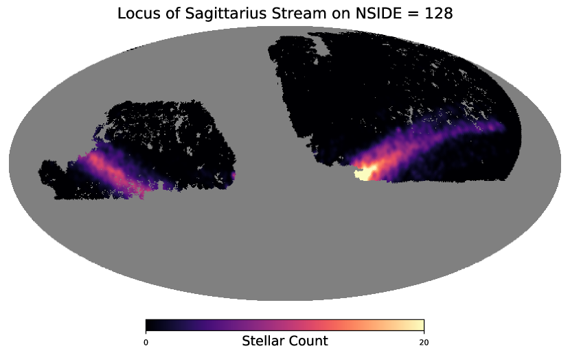
To best model the extent of the Sagittarius Stream, we consider the catalog produced by [60]777Data accessed: http://cdsarc.u-strasbg.fr/viz-bin/cat/J/A+A/666/A64 where they produce a sample of about candidate stars using the Gaia Early Data Release 3. However, only about stars fall within our footprint. As such, the locus of the Stream, as defined by these stars, is rather noisy. As such, we apply a Gaussian smoothing with on the Sagittarius Stream map and consider the smoothed map as one of our features, as shown in Figure 8.
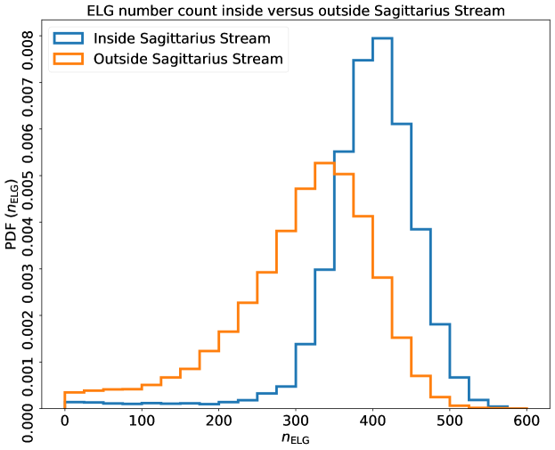
Figure 9 shows that the Stream affects the ELG number count; the ELG number density skews towards the right compared to the number density histogram outside the Stream. We also performed an Anderson-Darling test [61] to check whether the two samples were drawn from the same underlying distribution; the null hypothesis was rejected with a p-value . We use the Sagittarius Stream as one of the features in estimating the ELG galaxy window function.
4.5 Multiplicative Bias in Planck CMB Lensing
The Planck 2018 CMB lensing paper [34] mentions five main steps in lensing reconstruction; the final step refers to applying a multiplicative correction factor — this multiplicative correction factor arises due to some approximations and assumptions made in the prior steps. Below, we discuss the the approximations and assumptions of steps 3 and 4 which are relevant to this analysis.
In step 3, the Planck team subtracts the mean field and normalizes the lensing map. Masks and anisotropies bias the lensing reconstruction estimator. This bias, known as the mean field, is the map-level signal expected from the mask, noise, and other anisotropic features of the map in the absence of lensing. It is estimated using the quadratic estimator, also used for lensing reconstruction. Once subtracted, the map is normalized using an approximate isotropic normalization; this isotropic normalization is based on an analytic derivation for the whole sky [62]. Afterward, in step 4, the Planck team measured the lensing potential power spectrum of the reconstructed map and subtracted three separate sources of noise – that refers to the Gaussian noise even in the absence of lensing, that refers to the non-Gaussian noise, and the noise induced by point sources.
However, the approximate isotropic normalization applied prior to the noise subtraction is suboptimal (For further discussion, refer to Sections 2.1 and 2.3 of [34]) because the noise results in significant anisotropy. The isotropic approximations made earlier in Step 3 become a significant enough factor downstream. To fix this issue, the Planck team uses inhomogeneous filtering on their polarization data during reconstruction, drastically improving the lensing map. However, the inhomogeneous anisotropic filter results in a position-dependent (survey mask-dependent) normalization, or the multiplicative bias factor that we correct for when measuring the power spectrum.
We calculate the multiplicative renormalization factor using the method outlined in Reference [22]. In this procedure, we use the pairs of Planck lensing simulations that come with the CMB lensing data; each of these pairs has one simulation that is based on the pure CMB lensing convergence signal, while the other is a reconstruction of the lensing convergence signal in the presence of masks, noises, and other systematics. We can then apply the ELG mask on both the pure lensing convergence map and the reconstructed map and then take their ratio to estimate by how much the cross-power spectrum is biased per bin, i.e.,
| (4.11) |
where is a pure lensing convergence field simulation and is the corresponding reconstructed lensing convergence field.
Since is a ratio estimator, taking the mean of the ratio from the simulations is far noisier than taking the ratio of the mean of the pairs of power spectra. We describe in Section C the result of the multiplicative bias factor, , for different choices of the Galactic extinction map to correct the ELG overdensity. We multiply the measured power spectrum with this correction vector to obtain the debiased cross-power spectra.
In Appendix C, we show a detailed study to validate that the variance arising from estimating this multiplicative bias factor is subdominant to other systematics, such as photometric redshift uncertainty; as a result, we do not propagate the variance of estimating the multiplicative bias factor into our final covariance matrix.
Beyond the Monte Carlo norm correction there are two additional biases that may contribute to the cross-power spectrum measurement – 1) the bias and 2) the extragalactic foreground contamination in CMB lensing reconstruction. The bias refers to the contribution of the bispectrum induced by the non-linear growth of the large-scale structures and post-Born lensing; however the contribution of this bias at redshift around and also in the Planck lensing reconstruction is sub-percent level, [63] which is why we do not consider it. On the other hand, extragalactic foreground such as the cosmic infrared background and Sunyaev-Zeldovich clusters can affect the CMB lensing reconstruction estimator; however these biases are order of magnitudes smaller than the Planck CMB lensing primary noise [64], which is why we do not consider this bias either in our analysis.
5 Inference of Cosmological Parameters and The Covariance Matrix
Ultimately, we use the power spectra measurements to infer two cosmological and two galaxy bias parameters. The problem can be expressed in terms of Bayes’ Theorem:
| (5.1) |
where, is the data (in our case the two power spectra measurements), are the parameters we are interested in inferring (, and or ), is the posterior probability, is the likelihood function, and represents the prior probability of the parameters of interest.
The priors of the parameters are:
| (5.2) | ||||
| (5.3) | ||||
| (5.4) |
where and refer to uniform and Gaussian distributions respectively. We use broad uniform priors for , , and ; we set the bounds so that existing literature values are within the range. Note that we fix other cosmological parameters, i.e., , , , , , , , , , , and constant according to Table 2. The estimated magnification bias parameter, , is also fixed based on Section 4.2. Finally, the galaxy shot noise is also estimated using Equation 4.10 by taking the ensemble average over the window functions.
On the other hand, we model the likelihood as Gaussian because, according to the Central Limit Theorem, the likelihood will become Gaussian for scales much smaller than the survey size. As the DESI Legacy Imaging Surveys is about deg2, and the largest mode we use in our analysis is (or deg), the Gaussian likelihood is a good approximation. Thus, the logarithm of the likelihood is:
| (5.5) | ||||
where, refers to the binned pseudo- measurements of both galaxy-galaxy and galaxy-CMB lensing power spectra in a single vector, refers to the binned theoretical models and refers to the binned covariance matrix of the . The analysis is done in the range with equally spaced bins in the logarithmic space. We choose because that is the recommended small-scale cut used in the official Planck lensing paper. We also restrict our galaxy-galaxy power spectrum analysis to the same -space range to not be affected by mismodeling of non-linear effects at high-. The models, , are calculated using skylens, which in turn uses the power spectrum code camb [65] to calculate . For the non-linear correction, we use halofit [66] inside camb. Note that halofit agrees at the level of with state-of-the-art emulators and N-body simulations at Mpc-1 [67, 68]; it is the smallest scale probed by our analysis at the effective redshift of . At this scale, the non-linear correction is about compared to the linear matter power spectrum.
Note that the prefactor in front of the is the Hartlap correction [69] to obtain an unbiased estimate of the precision matrix (inverse of the covariance matrix), where refers to the number of simulations and refers to the number of bins. In this analysis, we set and since we have bins per power spectra.
| Fiducial Parameter | Value |
|---|---|
| [, , ] eV | |
| K | |
| Magnification Bias | |
| Shot noise | |
| 1.4 |
We estimate the covariance matrix using a simulation-based approach based on the method outlined in Reference [50]. We opt for a simulation-based approach rather than using a Gaussian analytic covariance matrix because we want to account for the variance of the galaxy window function and photometric redshifts so that we can marginalize over them. Briefly, we simulate pairs of correlated Gaussian mocks of the galaxy overdensity field and the CMB lensing convergence field and apply the ELG mask described in Section 4.3 and the CMB lensing mask provided by Planck.
While all of these simulations have the same baseline cosmology and galaxy biases (shown in Table 2), the individual simulations each have a different galaxy window function and redshift distribution, . We sample these window functions by taking snapshots of the neural network per training epoch, and we sample the as described in Section 3.4. Note that shown in Equation 4.10, a different realization of the galaxy window function yields a different estimate of the galaxy shot noise.
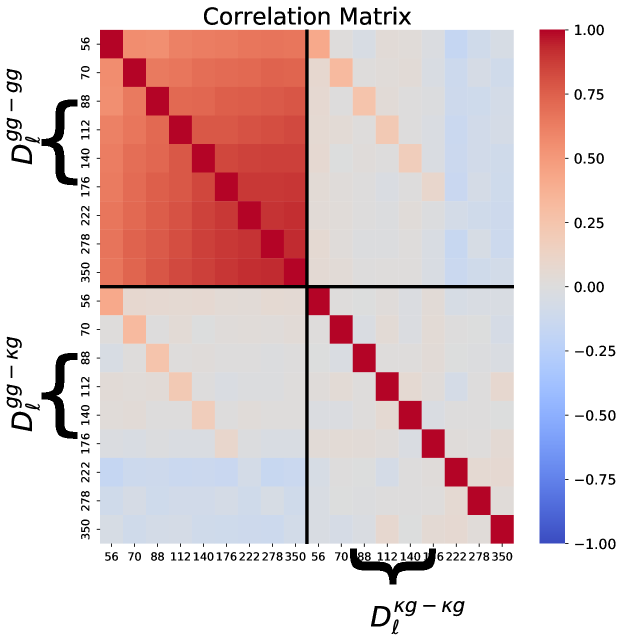
We then measure the and per simulation and calculate the covariance from these pairs of power spectra. Each of the measurements are also corrected for by its corresponding shot noise as discussed above. We show the corresponding correlation matrix of this covariance matrix in Figure 10 — the galaxy-galaxy power spectra portion of the covariance matrix exhibits high mode-mode coupling due to photometric redshift uncertainty. However, the covariance matrix is well-behaved with a condition number of about .
6 Validation with Gaussian Simulations
As we saw in Section 4, the analysis pipeline for the pseudo- measurements of the galaxy-galaxy and galaxy-CMB lensing power spectra are complicated. As a result, we must ensure that the final outputs of our pipeline are reasonable and make sense.
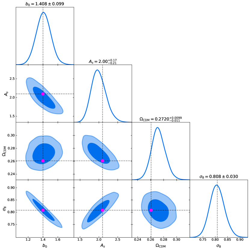
We use the correlated Gaussian mocks discussed in Section 5 to do this. These simulations have the same baseline cosmology and galaxy bias properties (shown in Table 2) but vary in galaxy window functions and photometric redshifts. We use the mean of these simulations as our validation mock. The posterior of the parameters of interest (Equation 5.1) is sampled using the Markov Chain Monte Carlo sampler emcee. The sampled posterior is shown in Figure 11; the dark-blue and the light-blue regions show the and the contours, respectively, while the dashed black lines and the magenta dots represent the truths. We see that the analysis pipeline can recover all the parameters of interest, with parameters , and having precisions of , and .
7 Results
We measure the galaxy-galaxy and galaxy-CMB lensing power spectra in the range with equally-spaced bins in logarithmic space. In our initial analysis, we used the Reference [57] (hereafter SFD) dust map as the tracer of Milky Way extinction in our foreground systematics modeling. However, during this time, we became aware of concerns that the SFD dust map might not be best suited for cosmological analyses, especially with ELGs, because the SFD map uses far-infrared emission to model Galactic extinction. However, the cosmic infrared background (CIB) is also bright in the far infrared. The CIB is a powerful tracer of high-redshift dusty galaxies such as ELGs. Hence, the SFD map may have some intrinsic signal that traces the ELG density field.
To better understand this effect, we reran our entire analysis using four additional dust maps – Reference [70] that uses the Sloan Digital Sky Survey to remove large-scale structure signals from the SFD dust map, Reference [71] thermal dust emission map, Reference [72] that uses stellar reddening from Pan-STARRS1 and 2MASS surveys, and Reference [73] that uses stellar reddening from Year DESI spectroscopic observations of halo stars. Although there are additional Galactic extinction maps, we chose these four because of their wide-area coverage and relatively high resolution. Hence, we report all our results in the following subsections by considering the different dust maps.
7.1 Power Spectra Analysis
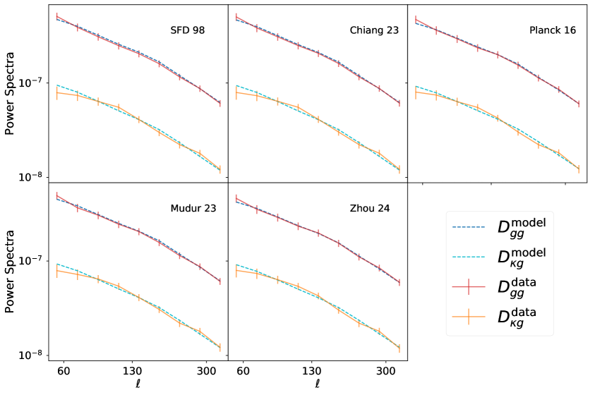
The measured power spectra, and , are shown in with solid lines in red and orange respectively in Figure 12, and the corresponding maximum a posteriori (MAP) estimated models are shown with dashed lines in navy and light blue. Each panel shows the MAP estimate as a function of the dust map used to estimate the galaxy window function. We note that the lowest bin, corresponding to the largest scale, generally has a poorer fit to the models compared to the rest of the power spectra. Section 8 offers possible explanations of what may be happening.
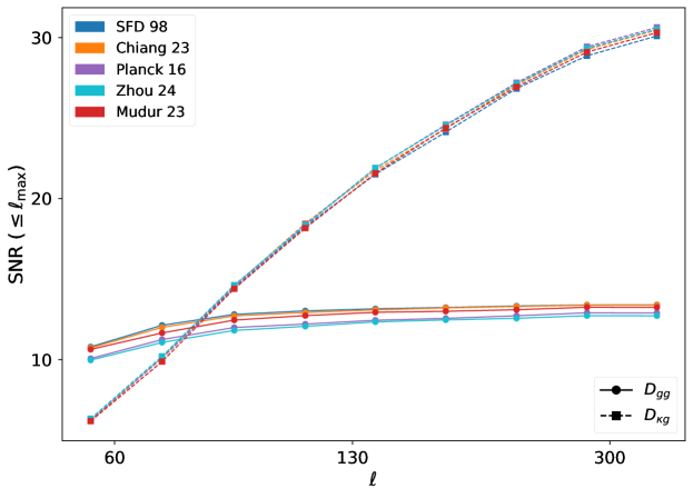
The corresponding cumulative detection significance can be seen in Figure 13, and we report a detection significance of ELG-ELG auto power spectra and a detection significance of ELG-CMB lensing cross power spectra. We calculated the detection significance as follows:
| (7.1) |
where refer to the power spectra measurements from the bin to the bin, and refer to the submatrix of the original covariance matrix (Figure 10) running from the bin to the bin in each direction.
The galaxy auto-power spectra significantly suffer due to the impact of photometric redshift uncertainty affecting the galaxy-galaxy auto-power spectra part of the covariance matrix. We confirmed this by measuring the cumulative signal-to-noise with a covariance matrix that does not have the photometric redshift uncertainty included in it; we saw that for such a covariance matrix, the galaxy-galaxy signal-to-noise can increase by an order of magnitude. Thus, our analysis shows that a robust marginalization of photometric redshift is paramount to get a high signal-to-noise measurement of the galaxy-galaxy power spectra.
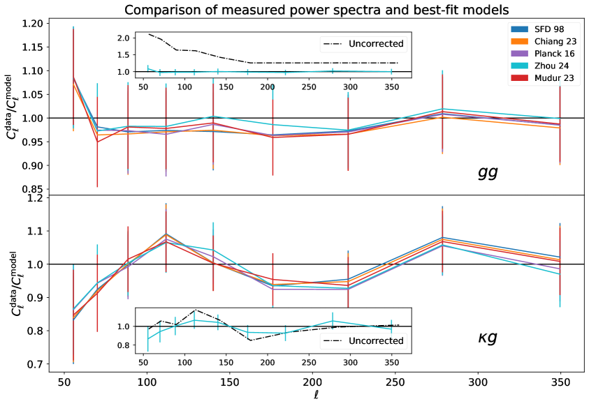
We also note that for galaxy-galaxy clustering, the galaxy window function or imaging systematics correction, were significant. Figure 14 shows a comparison of power spectra with respect to the best-fit models for the different dust maps. It also shows in the insets what the power spectra would look like if we had not corrected for the galaxy window function; in this case, the galaxy-galaxy auto-power spectrum is significantly affected at all scales, while the galaxy-CMB lensing cross-power spectrum is unaffected. As we discuss in detail in Section 8.2, not correcting for the galaxy window function affects most substantially. For the same , if the measured is higher than some reference value, then the inferred galaxy bias will also be higher and consequently, the inferred will be lower.
7.2 Parameter Inference
| Dust map | ||||
|---|---|---|---|---|
| SFD 98 [57] | ||||
| Chiang 23 [70] | ||||
| Planck 16 [71] | ||||
| Mudur 23 [72] | ||||
| Zhou 24 [73] |
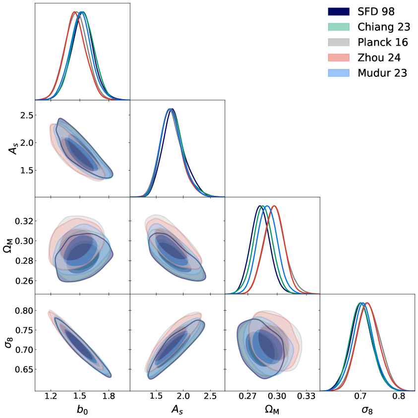
We show the final results and the posterior distributions in Figure 15. The sampling of the posterior is done in the , , parameter space while and are derived quantities from every MCMC proposal. We derive by adding the sampled to the fixed value of baryon density, , which is the best-fit value derived from Big Bang Nucleosynthesis measurement of ; here we fixed to the value shown in Table 2. Additionally, we fix other cosmological parameters constant to the fiducial model in Table 2 because the growth of structure measurements are the most sensitive to galaxy biases and a combination of and .
We measure the ELG galaxy bias to be in the range at . On the other hand, we measure cosmological parameters and to be in the ranges and respectively. The uncertainty on the inference of is roughly .
8 Discussions
In this section, we contextualize our findings with a few existing results in the literature and comment on how different systematics may play a role in the apparent tension that is persistent in the literature.
8.1 Comparing Result with Existing Measurements
One of the significant points of contention in the tension debate has to do with the high values that CMB experiments such as Planck and ACT have measured in comparison to low-redshift weak lensing and galaxy clustering surveys such as the Dark Energy Survey.
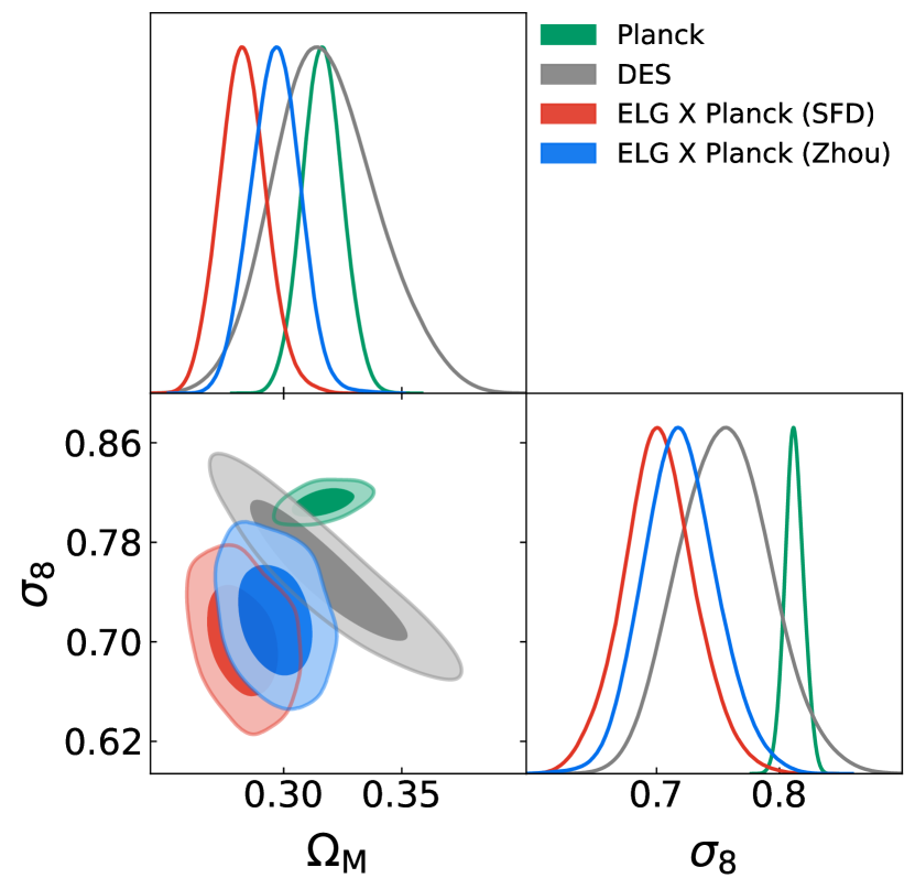
For context, the Planck 2018 paper reports ; this measurement is based on joint analysis of temperature, polarization, temperature cross polarization, and low multipole polarization data (TT, TE, EE + lowE). On the other hand, the DES Year paper reports ; this measurement is based on a joint analysis of -point correlation function using cosmic shear, galaxy clustering, and cross-correlation of cosmic shear with galaxy-galaxy lensing, BAO, and supernovae. Here we use the DES result as a representative result of other low-redshift surveys. The comparison of these results is shown in Figure 16. While the three surveys closely align on the estimation of , the picture is different for . Additionally, Figure 16 includes our measurements, specifically a contour where we used the SFD dust map to model the galaxy window function and another contour where we used the [73] dust map to model the same.
Two important things stand out from this plot. First, while our measurement of is not competitive with early-Universe experiments such as Planck (), our precision () is competitive with that of the Dark Energy Survey Year cosmology (), showcasing that future analyses with better ELG photometric redshift or spectroscopic redshift will have the ability to measure much more precisely.
Second, the choice of dust map has a noticeable effect on pulling the contour towards the Planck results. Since the posterior we are comparing with Planck primary anisotropy is two-dimensional ( plane), we can use the Mahalanobis distance [74], which is analogous to propagating errors for calculating differences in one-dimension:
| (8.1) |
where refer to the central values and refer to the parameter covariances. Since the problem is multidimensional, does not directly translate to the usual convention used in cosmology to quantify tension. Fortunately, follows the usual distribution, and we can use the numbers of degrees of freedom to calculate the associated -value and the associated value. Note that in this case, the answers the question: if I assume the value to be with the covariance , then how extreme is the point along the line that connects the two central values? Unlike the usual one-dimensional that only accounts for variances accounts for the often-ignored covariance information too.
| Data A | Data B | ||
|---|---|---|---|
| ELG Planck CMB lensing: SFD 98 [57] corrected | Planck Primary Anisotropy [8] | ||
| ELG Planck CMB lensing: Zhou 24 [73] corrected | Planck Primary Anisotropy [8] | ||
| DES Year [75] | Planck Primary Anisotropy [8] | ||
| ELG Planck CMB lensing: SFD 98 [57] corrected | DES Year [75] | ||
| ELG Planck CMB lensing: Zhou 24 [73] corrected | DES Year [75] | ||
| ELG Planck CMB lensing: Zhou 24 [73] corrected | ELG Planck CMB lensing: SFD 98 [57] corrected |
With this in mind, we report the discordance between parameters inferred using the SFD 98 [57] and the Zhou 24 [73] corrected ELG overdensity maps, and the Planck primary anisotropy [8] and DES Year [75] results in Table 4. We see that the choice of the Galactic extinction correction of the ELG overdensity field has a significant impact on our interpretation of whether there is a cosmological “tension” on the plane; SFD 98 based correction points towards a significantly higher discrepancy with Planck primary anisotropies compared to Zhou 24. Moreover, SFD 98 based correction also shows a noticeable tension with the DES Year results, while Zhou 24 based correction measurements do not.
Additional recent papers to compare to are the cross-correlation of the DESI luminous red galaxies photometric sample and ACT CMB lensing [20, 21], cross-correlation of the unWISE galaxy sample with Planck and ACT CMB lensing [22], the original unWISE cross-correlation with Planck CMB lensing [24] and the cross-correlation of the DESI-like luminous red galaxies (LRGs) sample from the Legacy Surveys with Planck CMB lensing [23]. Philosophically, these papers use ideas similar to ours in that they cross-correlate galaxy overdensity fields with CMB lensing maps. However, we note that the pipeline for this study was developed independently of these other papers. These papers use tomography to measure at different effective redshifts, with unWISE leaning towards a higher redshift than our sample and LRGs leaning towards a lower redshift than ours.
The most comparable sub-samples from unWISE and LRGs are the ”Green” and the pz_bin4 samples. The unWISE Green sample has a broad redshift kernel with a peak around , and the LRG pz_bin4 sample also has a broad redshift kernel with a peak around . [22] (ACT DR6 × unWISE + Planck PR4 × unWISE + BAO) and [24] (fixed ) measured using the unWISE Green sample to be and respectively. [23] measured to be (fixed ).
In all these examples, they prefer a much higher compared to our ELG-based measurements, and especially Reference [22] finds no tension with Planck. While the peculiarity between our results and these earlier works may be attributed to mismodeling galaxy-halo connection, our analysis is restricted to reasonably large scales ( implies at ). The agreement between the data and the best-fit models at smaller scales is strong.
One of our work’s major limitations is that we could not do a tomographic analysis because of sizeable photometric redshift calibration uncertainties. An important step forward to check whether the tension we have found in this paper is cosmological in origin or not, is by re-analyzing the CMB lensing and DESI ELG cross-correlation using spectroscopic redshifts, which we leave for a future paper.
8.2 Impact of Systematics on parameter inference
| Potential Systematics | Impacts ? | Impacts ? | Impact on and |
|---|---|---|---|
| Unaccounted LSS signal in dust map | Yes | Yes | Possible non-linear impact. See Appendix D.1 |
| Unaccounted local dust components in dust map | Yes | No | Infer to be higher and to be lower. See Appendix D.3 |
| Unaccounted stellar (stream) contaminants | Yes | No | Infer to be higher and to be lower. See Appendix D.3 |
| Not considering the full distribution of imaging systematics or the galaxy window function | Yes | No | Infer to be higher and to be lower. See [50] |
| CMB Lensing Monte Carlo Norm Correction | No | Yes | Infer to be lower and to be higher. See Appendix D.4 |
| Mismodeling of magnification bias | Yes | Yes | Possible non-linear impact. See Appendix D.2 |
As we saw in Figure 16, the choice of dust maps to modulate the galaxy window function has a significant impact on the inference of . Our careful studies of various systematics also indicate that different systematics can affect the observed galaxy-galaxy and galaxy-CMB lensing power spectra in specific ways, consequently affecting the inferred values of and .
To first order, we can use Equations 4.5 and 4.6 to understand how getting one (or both) of the power spectra modeling wrong affects the galaxy bias and . At least out of the systematics summarized in Table 5 show that they can lead to a lower inferred value of . We show derivations of these effects in Appendix D.
As cosmological surveys get more precise, previously unaccounted-for effects are becoming the dominant source of modeling mismatch, making the determination of cosmological parameters more challenging. First, observational systematics are best modeled using data-driven approaches. As these foreground systematics maps are generated using the maximum likelihood estimator approach, it has become crucial to marginalize over their probability distribution rather than considering only one value. Equally importantly, understanding the mutual information between the foreground systematics map made using different methods or datasets is also becoming necessary for uncertainty quantification. For example, both [70] and [73] are efforts to improve upon the SFD map, but they lead to different estimates of . Additionally, specific contaminants such as stellar streams are poorly constrained because our best model of them is limited by the number of stars associated with them. Hence, understanding these local, inter-Milky Way contaminants will be significant when we try to constrain cosmological models with galaxies at the flux limit of the telescopes.
Although we do not have quantitative evidence, Figure 12 hints that the lowest bin has the highest discrepancy with the best-fit models. Imaging systematics such as stellar streams and dust maps are typically large-scale, resulting in steeper observed power spectra at low values. Thus, we will need more comprehensive and robust foreground imaging systematics maps in the future if we want to use information from large scales. We also note that in the pseudo- framework, the worry is not restricted only to large scales; due to mode-mode coupling signal from large scales, it can also affect small scales.
Second, while many of these systematics have been treated independently of each other in the past, there is now a more pressing need for joint simulations to model them together. As discussed in Appendix C, we found non-zero covariances between the CMB lensing Monte Carlo norm correction factor and the galaxy window function. Although we could avoid modeling the covariance terms exactly since the errors are subdominant to photometric redshift uncertainties, any future survey with smaller photometric redshift uncertainties or spectroscopic redshifts may eventually need to account for this effect. Thus, we encourage the field to consider building joint correlated simulations of surveys to facilitate accurate cross-survey analysis.
9 Conclusions
In this paper, we have presented the first-ever cross-correlation analysis of CMB lensing with Emission-Line Galaxies to measure , and the ELG linear bias, . We find that the choice of Galactic Extinction map has a noticeable effect on pulling the contour towards the Planck results. Our analysis based on ELGs from the DESI Legacy Imaging Surveys and Planck CMB lensing showcase that ELG-type tracers will allow us to probe cosmological parameters in the high-redshift Universe with high precision. Technological and survey innovations such as the Legacy Surveys, DESI, and Planck have finally made this approach of probing the growth of structure viable.
This paper provides some important methodological developments in dealing with various sources of systematics that affect these kinds of cross-correlation analyses, namely:
-
•
We developed a fully forward-model pipeline that can use generative models of systematics to infer cosmological parameters using SkyLens.
-
•
We investigated various data-level systematics to obtain the cleanest ELG sample consisting of million galaxies.
-
•
We showcased a thorough analysis of ELG photometric redshift and their uncertainties using deep DESI Survey Validation data.
-
•
We showed that the Sagittarius Stream is a significant contaminant source in photometric ELG sample and we correct for its effect by using it as a template to model the galaxy window function.
-
•
We derived a simulation-based covariance matrix that considers various systematics, including marginalizing over the galaxy window function.
-
•
We devised a method to jointly estimate the covariance between the Monte Carlo norm correction systematics and the galaxy window functions.
-
•
We showcased how , , and are susceptible to the choice of dust maps used to estimate the galaxy window function.
The outcome of these advancements allowed us to measure competitively with other major weak lensing cross-correlation surveys such as DES. Our key results are:
-
•
The posterior estimate of the plane based on SFD correction indicates a tension with Planck, which is reduced to when we used the DESI stellar-reddening based correction. However, even using these maps results in tension with Planck, indicating that while dust can somewhat alleviate tension, it cannot do so completely.
- •
-
•
The detection significance of the galaxy-galaxy power spectrum was severely affected by photometric redshift uncertainties.
While we tried our best to account for various systematics and uncertainties, our experience has also taught us about things that can be improved upon in the future and can help ELG-based photometric surveys with their analysis design. The main limitations of our work are as follows:
-
•
We were ultimately affected the most by photometric redshift uncertainties in our modeling. The DESI Legacy Imaging Surveys have only three broadband filters, so we could do little to improve this. Additionally, we could not account the redshift distribution of about of our sample which led to us using a long-tail redshift distribution. Our work shows the need for spectroscopic analysis for galaxies with a limited number of identifiable lines in the observed frame wavelength. It also shows that narrow-band photometry is paramount to reducing the impact of photometric redshift uncertainty in cosmological analyses.
-
•
We also have used a relatively simple galaxy linear bias model for ELGs as we restricted our analysis to relatively large scales. However, recent studies that use more massive galaxies such as luminous red galaxies have shown that one can use Lagrangian Perturbation Theory and the Effective Field Theory of the Large-Scale Structures to extract information from much smaller scales [21, 22, 80, 23]. However, initial data from DESI has shown that the small-scale clustering of ELGs are affected by conformity bias and a higher satellite velocity dispersion [81]. Hence, extending either the Perturbation Theory or the Halo-Occupation Distribution approaches to DESI ELGs will require careful modeling of small-scale clustering, especially if the goal is to use next-generation CMB lensing maps such as the ACT CMB lensing map. We leave this task for a future paper.
-
•
Computational resources limited our estimation of the window function posterior. On the computation side, it took us a week to sample unique window realizations from the neural networks. We would like to use many more realizations to reduce the noise due to a finite number of realizations. Additionally, sampling the posterior of a neural network is still an active area of research, and many different methods are in use. As these methods improve, the galaxy window functions’ modeling quality will also improve.
-
•
We used Gaussian simulations to estimate the covariance matrix. Although our method is robust because it considers effects such as photometric redshift and window function uncertainties, it does not account for non-Gaussian contributions to the covariance due to the nature of our baseline simulation. A similar covariance estimation based on -body simulations will capture non-Gaussian components we currently fail to capture.
-
•
We used five different dust maps to get cosmological parameter estimates, but we did not make any scientific judgments on which dust map is the “best” one.
Ultimately, the ELGs have opened up a new era of cosmological analysis. With ongoing and future ELG-based surveys such as DESI, Euclid [82], Roman [83], SPHEREx [84] and the Rubin Observatory [85], as well as CMB lensing surveys such as the Simons Observatory [86] and CMB-S4 [87], it is only a matter of time before we begin to explore the growth of structure in multiple high redshift epochs tomographically.
Appendix A Functional Form of the Exponential Decay Function
In this section, we will derive the functional form of an exponential decay function whose first point and the overall area under the curve are given.
Let be the first point (correspond to the midpoint bin value and the histogram value of the last histogram of the redshift distribution curve obtained using Random Forest Classifier), and be the area under the exponential decay distribution. Thus, we can write the usual form of exponential decay distribution as:
We need to solve for the parameter . If is the area under the curve of , then we can write the following:
| (A.1) |
We will now apply a change of variable such that . This changes the Equation A.1 to:
Thus, if the last bin value and the area under the exponential curve are known, we can write the functional form of the exponential decay distribution as:
| (A.2) |
Appendix B Stellar and Foreground Galaxy Masks
Large-scale structure surveys have to use masks to block out areas around stars and bright foreground galaxies because they can introduce artificial signals in the power spectrum measurement. Bright foreground objects can preferentially block out fainter background objects, distorting the galaxy number count and number density. As a result, a certain amount of area around these objects is completely masked out when preparing large-scale structure catalogs. A similar step was taken with the DR9 Legacy Surveys ELG catalog when identifying potential DESI targets based on galaxy photometry.
However, when we ran our regression analysis to model the galaxy window function, we found that specific outlier pixels confused the regression model because there were an unusually large number of ELGs in these pixels. We isolated some of the most extreme pixels and visually inspected these fields using the pixel right ascension and declination. We used the Legacy Survey Viewer888https://www.legacysurvey.org/viewer, which is a website built by the Legacy Surveys team containing imaging of the entire Legacy Surveys footprint and also includes value-added catalogs such as all the DESI-like ELG targets.
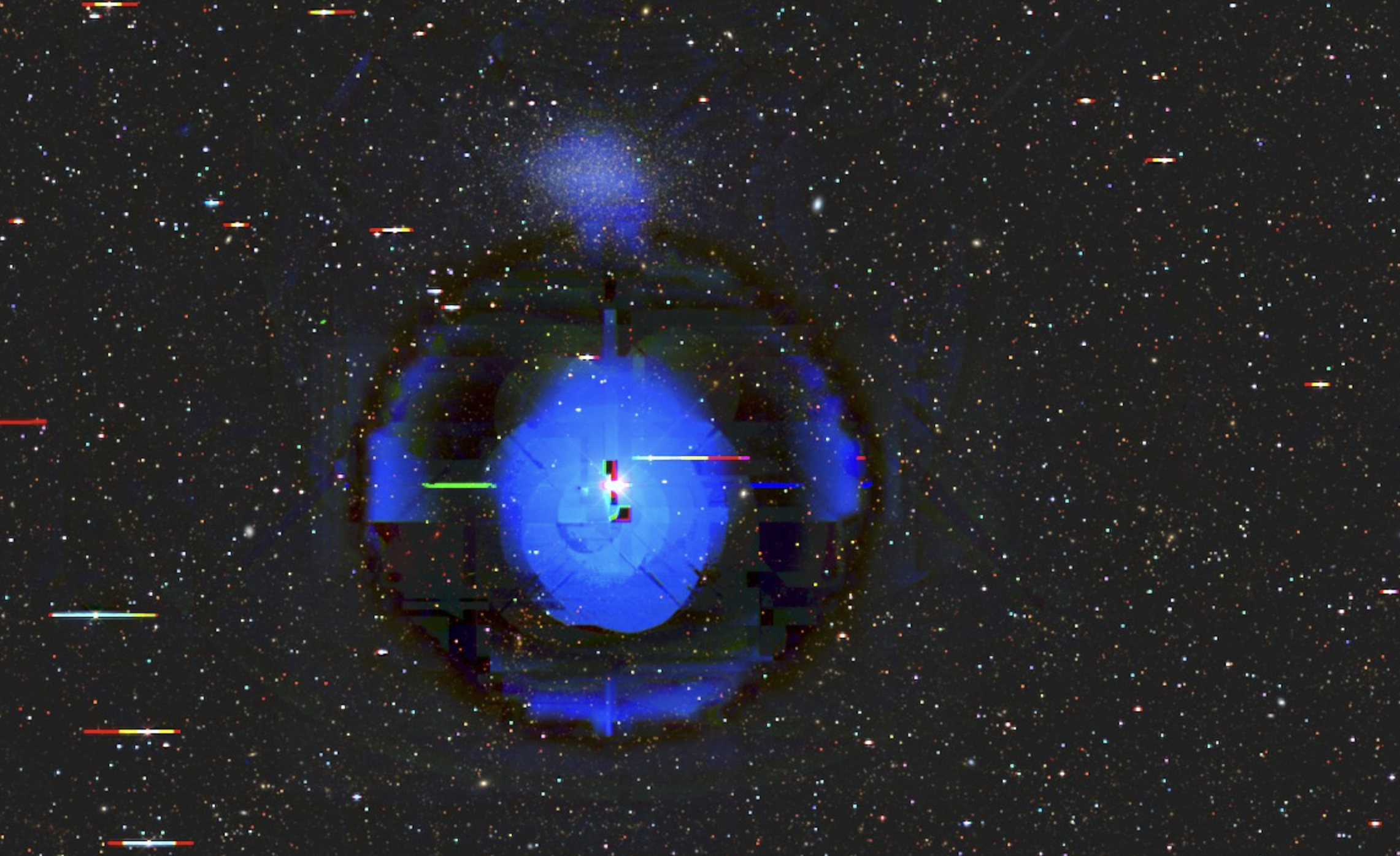
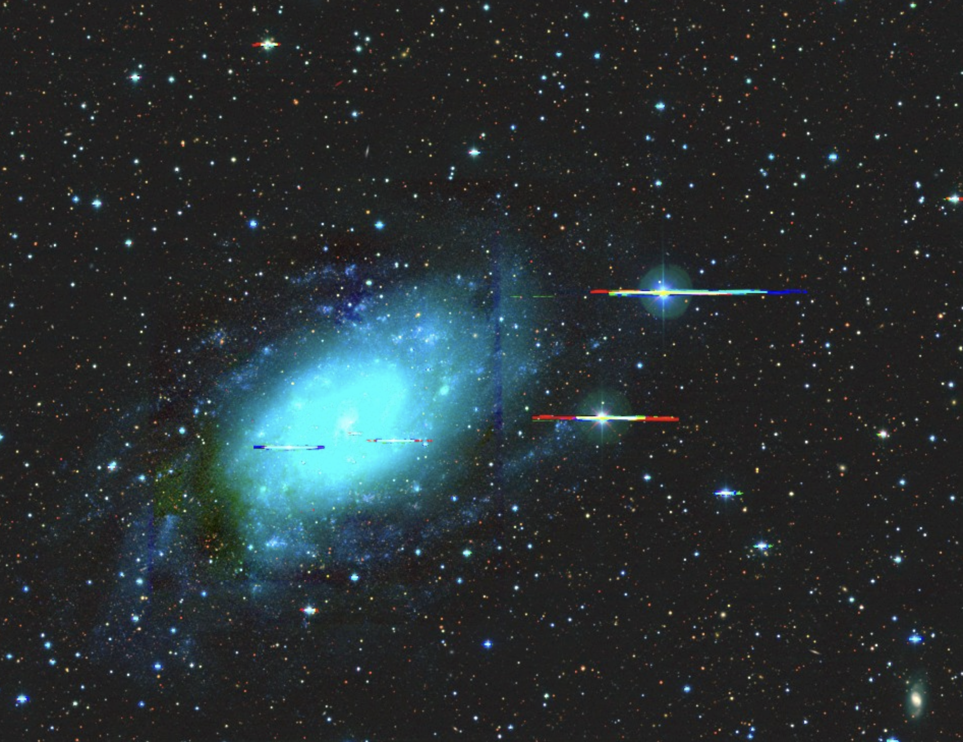
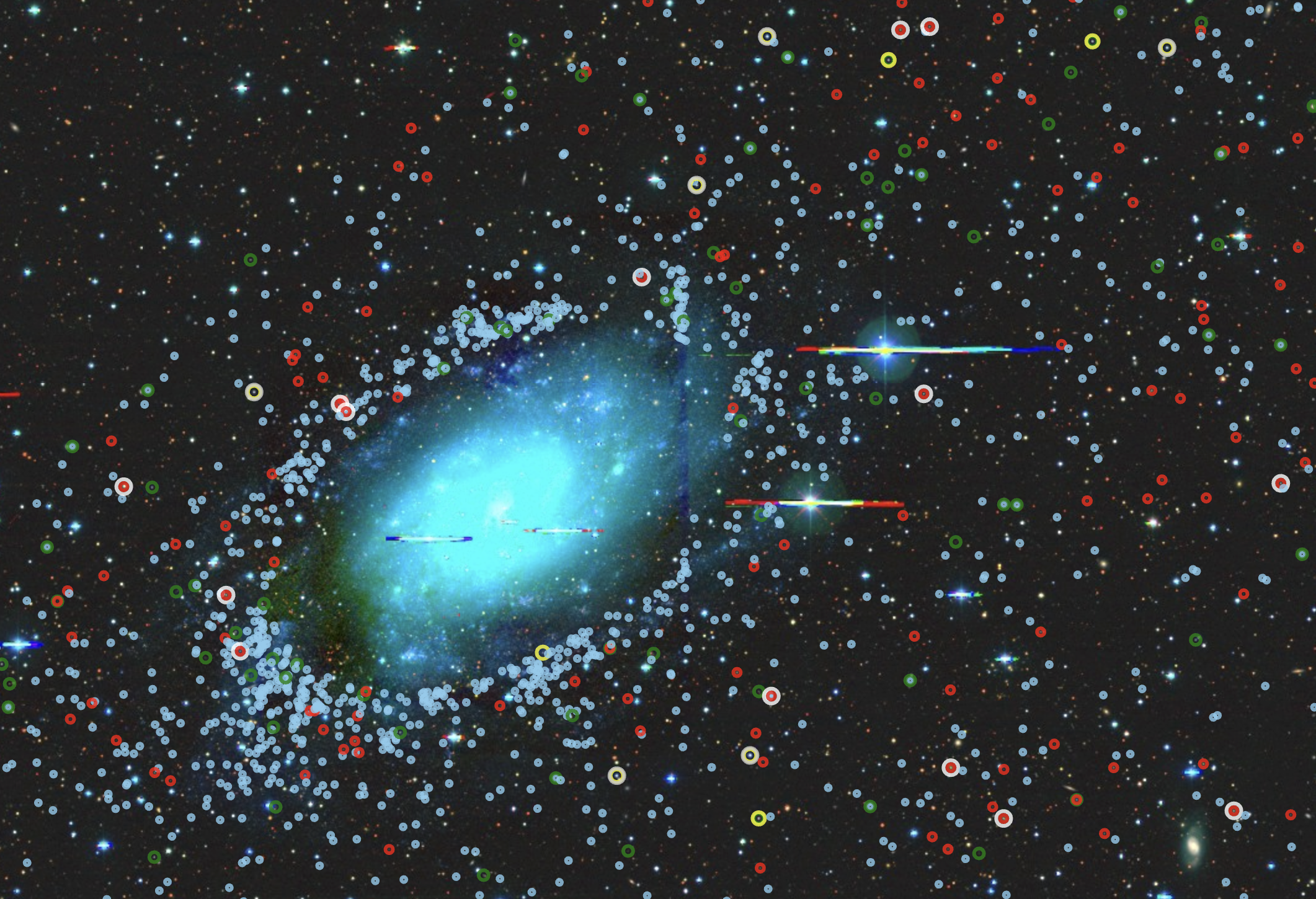
Figure 17 shows two such examples. Here, we show a bright star, *alf Leo, and an overlapping diffuse galaxy, Z 64-73, in the top panel and a bright foreground galaxy, NGC 2403, in the bottom. Ideally, the DESI target catalog would have masked out these objects properly. However, the right column in the figure clearly shows ELG targets (shown in blue circles) inside the diffraction arc of the star. The diffuse light of both galaxies mimics ELG targets, exemplifying a case where the large-scale structure catalog is affected by artificial ELGs, leading us to investigate this issue statistically and implement more conservative stellar and foreground galaxy masks.
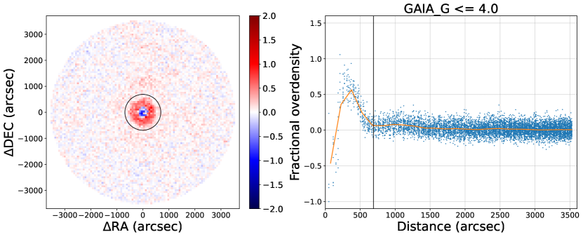

We used the Gaia [88] and the Siena Galaxy Atlas999https://www.legacysurvey.org/sga/sga2020/ [41] to identify stars and foreground galaxies in our footprint. We built the new stellar and galactic masks separately, but the analysis procedure was the same. To build the new masks, we binned the objects by their band magnitude, and the width of the bin was magnitude. We then centered all of these binned objects and stacked them together. Afterward, we picked radii of arcsec, depending on the brightness of the bin. We then calculate the fractional overdensity of ELG targets inside this radius. The expectation is that the ELG overdensity field around foreground objects should be a function of radius. If we detect a radial dependency, we increase the mask size for that bin until we do not see any radial dependency outside of the mask. Figure 18 shows an example of the brightest stars () from the Gaia catalog. It shows that we must apply to masks as large as in radius to remove such artificial number density fluctuations.
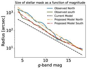
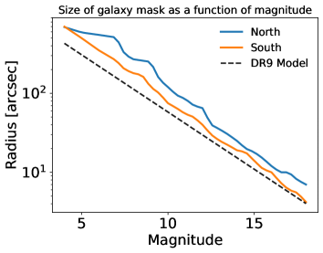
We show the summary of this exercise in Figure 19, which shows the relationship between mask size and the magnitude of the stellar and foreground galaxy contaminants. Notably, the DR9 mask size (in the black dashed line) is inadequate for large-scale structure analysis. The resulting radius vs. g-band mag curves fit the data better, and we use these models to construct our survey mask.
Appendix C Uncertainty of the Multiplicative Bias Estimator due to Planck CMB Lensing
As explained in Section 4.5, the Planck Collaboration (also other experiments such as the Atacama Cosmology Telescope [22]) make some assumptions about the CMB lensing noise properties which makes cross-power spectrum unbiased as long as the galaxy mask is the same as the CMB lensing mask. However, this is not true for almost all cases, including ours, so we must estimate the correction factor by considering a new galaxy mask. Because the noise property that the lensing reconstruction is optimized for is a function of sky position, we change the optimality of the default Planck lensing reconstruction by masking additional parts of the sky.
Suppose we know our CMB lensing and galaxy masks. In that case, we can use the pairs Planck CMB lensing simulations where each pair consists of one simulation with a pure CMB lensing convergence signal, , and one simulation of the associated reconstruction of the lensing signal by taking into account various noise properties, denoted as . The correction factor, is then given by:
| (C.1) |
Since the actual Planck CMB lensing map is a lensing reconstruction, we have to multiply the correction factor, , to get an estimation of what the true cross-power spectra, , ought to be. Note that both the numerator and the denominator are estimators since the field and the associated reconstructed field are estimated using the simulations. As such, is a ratio estimator, and estimating by taking ratios over all simulations and then taking the mean has a high variance. Instead, we choose to estimate by taking the ratio of the means of all the simulations, i.e.,
| (C.2) |
However, beyond this issue, the subtlety in our paper is that we treat the galaxy window function, , or the imaging weights as the effective mask such that our galaxy mask is no longer binary but has a continuous value in the range . In Section 4.4 and in our companion paper [50], we show how the estimation of can have biases and the uncertainty in estimating must be marginalized over to get the proper covariance matrix. As a result, the numerators and the denominators in Equation C.2, and consequently , vary not only due to the variance in and , but also due to the variance in the galaxy mask. Thus, we have to properly account for the covariance between realizations of and the galaxy window function to understand the noise properties of the estimator.
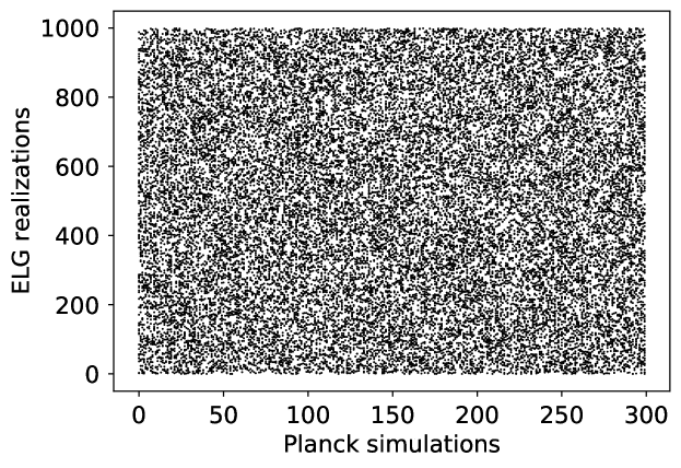
To explore this problem, we consider bootstrapped realizations of ; in each bootstrap realization, we randomly sample with replacements Planck and simulations with replacement as well as realizations of the galaxy window function, . We then use Equation C.2 to estimate . The bootstrapped realizations have enough coverage along both the Planck simulations of the ELG window function realizations to yield a robust answer, as shown in Figure 20.
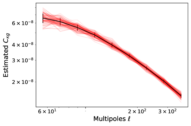
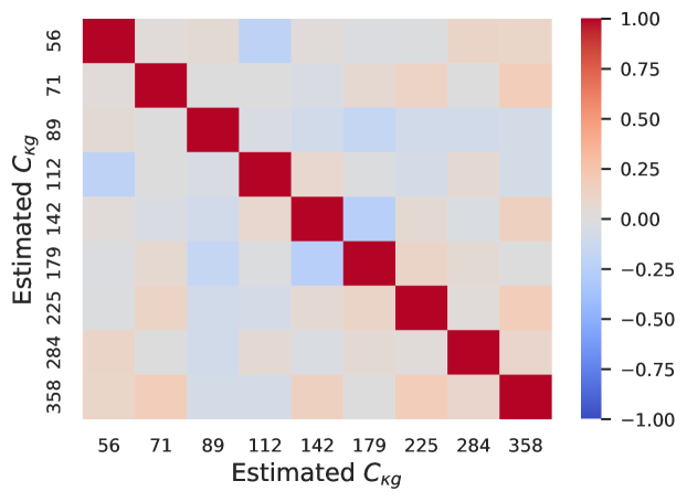
Finally, we need to convert the estimations of to estimations of to get a sense of how varying the Planck CMB lensing simulations and the ELG galaxy window functions jointly affect the estimator. For each realization, we randomly select one cross-power spectrum between the reconstructed lensing field, and the galaxy window function and estimate the corrected . Figure 21 shows the distribution of the estimated , and the corresponding covariance matrix is shown in Figure 22. The covariance matrix shows non-negligible off-diagonal terms, especially at high . This finding validates the concern that we should consider the joint covariance of the variance in CMB lensing simulations and the galaxy window function.
However, it is difficult to combine this covariance matrix properly with the covariance matrix we estimate in Figure 10 because while in Figure 10, we vary both and , in Figure 22 we vary the Planck CMB lensing simulations and ; for the latter does not directly enter in the analysis. Hence, combining these two covariance matrices becomes an intractable problem without a joint cross-survey simulation. As a side note, this kind of joint systematics analysis will become more critical in future cosmological papers. So, it merits the field to develop joint, correlated cross-survey simulations for proper forward modeling.
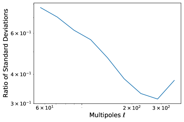
Nonetheless, the variance (and the covariance) due to the multiplicative bias can be avoided as in our analysis because Figure 23 shows that the error bars due to the multiplicative biases are only that of the error bars due to photometric redshift uncertainties. Hence, we do not propagate the error and consider only the average value. We do caution that for spectroscopic surveys where the redshift uncertainty is orders of magnitude smaller, this effect should be reassessed to ensure that it is subdominant; otherwise, one may have artificially smaller error bars than what they ought to be.
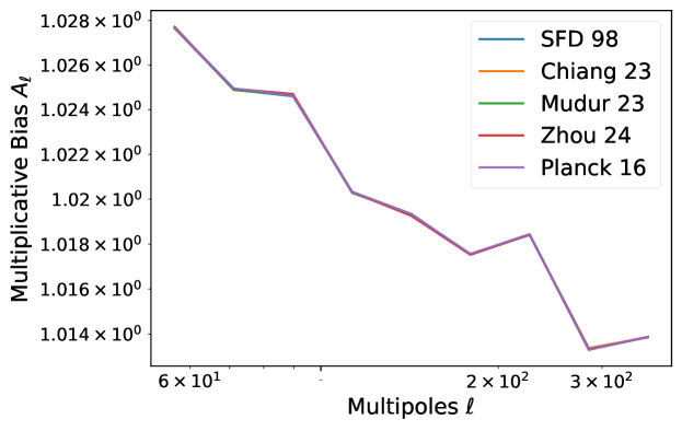
Finally, Figure 24 shows that no matter our choices of the Galactic Extinction map to estimate the galaxy window function, the multiplicative correction factor remains almost the same.
Appendix D Impact of Unaccounted Systematics on galaxy bias and
This appendix shows the theoretical calculations that helped us interpret the various systematics, primarily those described in Table 5.
D.1 Unaccounted LSS signal in foreground dust maps
In this situation, we consider a dust map that may have unaccounted large-scale structures (LSS) signal, e.g., we may have not accounted for large-scale structure due to cosmic infrared background contaminating the SFD dust map.
Here, we assume that our best estimate of the galaxy window function, , is composed of the pure, strictly foreground systematics (), and a part that is correlated with the LSS (). Using this information, we calculate observed power spectra and note from Equations 4.5 and 4.6 that to the first order, the linear bias is a ratio of them.
Hence, the inferred linear bias is:
If we expect the correlated part of the galaxy window function, to be small, we can then Taylor expand around :
Plugging this expansion into we get:
| (D.1) | ||||
| (D.2) | ||||
| (D.3) | ||||
| (D.4) |
we cancel the final term in the second line because the numerator is a minimal term. In the final expression, we see that our inferred linear bias is composed of the linear bias we are interested in measuring plus some linear and non-linear terms of various powers. Depending on the strength of the contamination, the inferred bias could either be higher or lower than the actual bias.
D.2 Unaccounted Magnification Bias signal in field
Next, we consider a situation in which we have not adequately modeled the magnification bias. As a result, our observed galaxy overdensity field is composed of the galaxy overdensity field we modeled properly and an additional term representing the unmodeled galaxies that are still contributing to our density field.
We similarly calculate the power spectra under these assumptions:
Hence, the inferred linear bias is:
As we assumed in the first subsection, if we expected the unmodeled part, to be small, then we can Taylor expand the denominator around :
Plugging this expansion into we get:
we cancel the final term in the second line because the numerator is very small. In the final expression, we see that the inferred bias is composed of the bias we are interested in measuring plus additional terms that can either increase or decrease the inferred value of the bias.
D.3 Unaccounted stellar (stream) or local dust contaminants
In this case, we consider a situation in which we have not adequately modeled stellar contaminants, and as a result, stars with similar colors as our galaxy sample masquerading as galaxies. We also consider a situation in which our dust map does not have leakage from the LSS but has unmodeled parts. For example, a poor modeling of the zodiacal light will leave an imprint of the residual zodiacal light.
As a result, our estimated galaxy overdensity field will be composed of the actual galaxy overdensity field and some additional contaminant field, .
We calculate the observed power spectra:
Hence, the inferred linear bias is:
Here, we see a clear excess signal that makes the inferred linear bias greater than the actual bias. Moreover, if the inferred bias is larger, the inferred will correspondingly be lower.
D.4 Unaccounted MC Norm Correction
In this case, we consider the situation where the Monte Carlo Norm correction is not accounted for when debiasing the observed galaxy-CMB lensing power spectra. As discussed in Appendix C, not accounting for the norm correction bias leads to a slightly lower value of the observed . If we consider the observed to be composed of the true cross-power spectrum and the correction factor, then:
Hence, the inferred bias is:
Thus, the inferred bias will be scaled by the norm correction factor.
Acknowledgments
The authors thank Rongpu Zhao, Gerrit Farren, Lukas Wenzl and Renée Hloz̆ek for their valuable discussions. The authors also thank Noah Sailer, Abhishek Maniyar, James Rohlf and Antonella Palmese for providing valuable feedback during the DESI internal review process.
TK is supported by the Arts & Science Postdoctoral Fellow at the University of Toronto. TK was supported by the National Science Foundation Graduate Research Fellowship under Grant No. DGE - 1745303 and the Barbara Bell Dissertation Fellowship at the Harvard University during part of this project. SS is supported by the McWilliams Fellowship at the Carnegie Mellon University. MR is supported by the U.S. Department of Energy grants DE-SC0021165 and DE-SC0011840.
This material is based upon work supported by the U.S. Department of Energy (DOE), Office of Science, Office of High-Energy Physics, under Contract No. DE–AC02–05CH11231, and by the National Energy Research Scientific Computing Center, a DOE Office of Science User Facility under the same contract. Additional support for DESI was provided by the U.S. National Science Foundation (NSF), Division of Astronomical Sciences under Contract No. AST-0950945 to the NSF’s National Optical-Infrared Astronomy Research Laboratory; the Science and Technology Facilities Council of the United Kingdom; the Gordon and Betty Moore Foundation; the Heising-Simons Foundation; the French Alternative Energies and Atomic Energy Commission (CEA); the National Council of Humanities, Science and Technology of Mexico (CONAHCYT); the Ministry of Science, Innovation and Universities of Spain (MICIU/AEI/10.13039/501100011033), and by the DESI Member Institutions: https://www.desi.lbl.gov/collaborating-institutions. Any opinions, findings, and conclusions or recommendations expressed in this material are those of the author(s) and do not necessarily reflect the views of the U. S. National Science Foundation, the U. S. Department of Energy, or any of the listed funding agencies.
The authors are honored to be permitted to conduct scientific research on Iolkam Du’ag (Kitt Peak), a mountain with particular significance to the Tohono O’odham Nation.
The DESI Legacy Imaging Surveys consist of three individual and complementary projects: the Dark Energy Camera Legacy Survey (DECaLS), the Beijing-Arizona Sky Survey (BASS), and the Mayall z-band Legacy Survey (MzLS). DECaLS, BASS and MzLS together include data obtained, respectively, at the Blanco telescope, Cerro Tololo Inter-American Observatory, NSF’s NOIRLab; the Bok telescope, Steward Observatory, University of Arizona; and the Mayall telescope, Kitt Peak National Observatory, NOIRLab. NOIRLab is operated by the Association of Universities for Research in Astronomy (AURA) under a cooperative agreement with the National Science Foundation. Pipeline processing and analyses of the data were supported by NOIRLab and the Lawrence Berkeley National Laboratory. Legacy Surveys also uses data products from the Near-Earth Object Wide-field Infrared Survey Explorer (NEOWISE), a project of the Jet Propulsion Laboratory/California Institute of Technology, funded by the National Aeronautics and Space Administration. Legacy Surveys was supported by: the Director, Office of Science, Office of High Energy Physics of the U.S. Department of Energy; the National Energy Research Scientific Computing Center, a DOE Office of Science User Facility; the U.S. National Science Foundation, Division of Astronomical Sciences; the National Astronomical Observatories of China, the Chinese Academy of Sciences and the Chinese National Natural Science Foundation. LBNL is managed by the Regents of the University of California under contract to the U.S. Department of Energy. The complete acknowledgments can be found at https://www.legacysurvey.org/.
References
- [1] S. Perlmutter, G. Aldering, G. Goldhaber, R.A. Knop, P. Nugent, P.G. Castro et al., Measurements of and from 42 High-Redshift Supernovae, ApJ 517 (1999) 565 [astro-ph/9812133].
- [2] A.G. Riess, A.V. Filippenko, P. Challis, A. Clocchiatti, A. Diercks, P.M. Garnavich et al., Observational Evidence from Supernovae for an Accelerating Universe and a Cosmological Constant, AJ 116 (1998) 1009 [astro-ph/9805201].
- [3] P. de Bernardis, P.A.R. Ade, J.J. Bock, J.R. Bond, J. Borrill, A. Boscaleri et al., A flat Universe from high-resolution maps of the cosmic microwave background radiation, Nature 404 (2000) 955 [astro-ph/0004404].
- [4] S. Hanany, P. Ade, A. Balbi, J. Bock, J. Borrill, A. Boscaleri et al., MAXIMA-1: A Measurement of the Cosmic Microwave Background Anisotropy on Angular Scales of 10’-5°, ApJ 545 (2000) L5 [astro-ph/0005123].
- [5] D.J. Eisenstein, I. Zehavi, D.W. Hogg, R. Scoccimarro, M.R. Blanton, R.C. Nichol et al., Detection of the Baryon Acoustic Peak in the Large-Scale Correlation Function of SDSS Luminous Red Galaxies, ApJ 633 (2005) 560 [astro-ph/0501171].
- [6] J. Rhodes, S. Allen, B.A. Benson, T. Chang, R. de Putter, S. Dodelson et al., Exploiting Cross Correlations and Joint Analyses, arXiv e-prints (2013) arXiv:1309.5388 [1309.5388].
- [7] D. Huterer, D. Kirkby, R. Bean, A. Connolly, K. Dawson, S. Dodelson et al., Growth of cosmic structure: Probing dark energy beyond expansion, Astroparticle Physics 63 (2015) 23 [1309.5385].
- [8] Planck Collaboration, N. Aghanim, Y. Akrami, F. Arroja, M. Ashdown, J. Aumont et al., Planck 2018 results. I. Overview and the cosmological legacy of Planck, A&A 641 (2020) A1 [1807.06205].
- [9] S. Aiola, E. Calabrese, L. Maurin, S. Naess, B.L. Schmitt, M.H. Abitbol et al., The Atacama Cosmology Telescope: DR4 maps and cosmological parameters, J. Cosmology Astropart. Phys 2020 (2020) 047 [2007.07288].
- [10] A.G. Riess, W. Yuan, L.M. Macri, D. Scolnic, D. Brout, S. Casertano et al., A Comprehensive Measurement of the Local Value of the Hubble Constant with 1 km s-1 Mpc-1 Uncertainty from the Hubble Space Telescope and the SH0ES Team, ApJ 934 (2022) L7 [2112.04510].
- [11] A. Porredon, M. Crocce, J. Elvin-Poole, R. Cawthon, G. Giannini, J. De Vicente et al., Dark Energy Survey Year 3 results: Cosmological constraints from galaxy clustering and galaxy-galaxy lensing using the MagLim lens sample, arXiv e-prints (2021) arXiv:2105.13546 [2105.13546].
- [12] S. Pandey, E. Krause, J. DeRose, N. MacCrann, B. Jain, M. Crocce et al., Dark Energy Survey year 3 results: Constraints on cosmological parameters and galaxy-bias models from galaxy clustering and galaxy-galaxy lensing using the redMaGiC sample, Phys. Rev. D 106 (2022) 043520 [2105.13545].
- [13] M. Asgari, C.-A. Lin, B. Joachimi, B. Giblin, C. Heymans, H. Hildebrandt et al., KiDS-1000 cosmology: Cosmic shear constraints and comparison between two point statistics, A&A 645 (2021) A104 [2007.15633].
- [14] C. Hikage, M. Oguri, T. Hamana, S. More, R. Mandelbaum, M. Takada et al., Cosmology from cosmic shear power spectra with Subaru Hyper Suprime-Cam first-year data, PASJ 71 (2019) 43 [1809.09148].
- [15] M.M. Ivanov, Cosmological constraints from the power spectrum of eBOSS emission line galaxies, Phys. Rev. D 104 (2021) 103514 [2106.12580].
- [16] S. Alam, M. Aubert, S. Avila, C. Balland, J.E. Bautista, M.A. Bershady et al., Completed SDSS-IV extended Baryon Oscillation Spectroscopic Survey: Cosmological implications from two decades of spectroscopic surveys at the Apache Point Observatory, Phys. Rev. D 103 (2021) 083533 [2007.08991].
- [17] T.M.C. Abbott, M. Aguena, A. Alarcon, S. Allam, S. Allen, J. Annis et al., Dark Energy Survey Year 1 Results: Cosmological constraints from cluster abundances and weak lensing, Phys. Rev. D 102 (2020) 023509 [2002.11124].
- [18] A.B. Mantz, A. von der Linden, S.W. Allen, D.E. Applegate, P.L. Kelly, R.G. Morris et al., Weighing the giants - IV. Cosmology and neutrino mass, MNRAS 446 (2015) 2205 [1407.4516].
- [19] E. Abdalla, G.F. Abellán, A. Aboubrahim, A. Agnello, Ö. Akarsu, Y. Akrami et al., Cosmology intertwined: A review of the particle physics, astrophysics, and cosmology associated with the cosmological tensions and anomalies, Journal of High Energy Astrophysics 34 (2022) 49 [2203.06142].
- [20] J. Kim, N. Sailer, M.S. Madhavacheril, S. Ferraro, I. Abril-Cabezas, J.N. Aguilar et al., The Atacama Cosmology Telescope DR6 and DESI: Structure formation over cosmic time with a measurement of the cross-correlation of CMB Lensing and Luminous Red Galaxies, arXiv e-prints (2024) arXiv:2407.04606 [2407.04606].
- [21] N. Sailer, J. Kim, S. Ferraro, M.S. Madhavacheril, M. White, I. Abril-Cabezas et al., Cosmological constraints from the cross-correlation of DESI Luminous Red Galaxies with CMB lensing from Planck PR4 and ACT DR6, arXiv e-prints (2024) arXiv:2407.04607 [2407.04607].
- [22] G.S. Farren, A. Krolewski, N. MacCrann, S. Ferraro, I. Abril-Cabezas, R. An et al., The Atacama Cosmology Telescope: Cosmology from Cross-correlations of unWISE Galaxies and ACT DR6 CMB Lensing, ApJ 966 (2024) 157 [2309.05659].
- [23] M. White, R. Zhou, J. DeRose, S. Ferraro, S.-F. Chen, N. Kokron et al., Cosmological constraints from the tomographic cross-correlation of DESI Luminous Red Galaxies and Planck CMB lensing, J. Cosmology Astropart. Phys 2022 (2022) 007 [2111.09898].
- [24] A. Krolewski, S. Ferraro and M. White, Cosmological constraints from unWISE and Planck CMB lensing tomography, J. Cosmology Astropart. Phys 2021 (2021) 028 [2105.03421].
- [25] F. Bianchini, A. Lapi, M. Calabrese, P. Bielewicz, J. Gonzalez-Nuevo, C. Baccigalupi et al., Toward a Tomographic Analysis of the Cross-Correlation between Planck CMB Lensing and H-ATLAS Galaxies, ApJ 825 (2016) 24 [1511.05116].
- [26] M.S. Madhavacheril, F.J. Qu, B.D. Sherwin, N. MacCrann, Y. Li, I. Abril-Cabezas et al., The Atacama Cosmology Telescope: DR6 Gravitational Lensing Map and Cosmological Parameters, ApJ 962 (2024) 113 [2304.05203].
- [27] A. Dey, D.J. Schlegel, D. Lang, R. Blum, K. Burleigh, X. Fan et al., Overview of the DESI Legacy Imaging Surveys, AJ 157 (2019) 168 [1804.08657].
- [28] DESI Collaboration, B. Abareshi, J. Aguilar, S. Ahlen, S. Alam, D.M. Alexander et al., Overview of the Instrumentation for the Dark Energy Spectroscopic Instrument, AJ 164 (2022) 207 [2205.10939].
- [29] DESI Collaboration, A. Aghamousa, J. Aguilar, S. Ahlen, S. Alam, L.E. Allen et al., The DESI Experiment Part II: Instrument Design, arXiv e-prints (2016) arXiv:1611.00037 [1611.00037].
- [30] J.H. Silber, P. Fagrelius, K. Fanning, M. Schubnell, J.N. Aguilar, S. Ahlen et al., The Robotic Multiobject Focal Plane System of the Dark Energy Spectroscopic Instrument (DESI), AJ 165 (2023) 9 [2205.09014].
- [31] T.N. Miller, P. Doel, G. Gutierrez, R. Besuner, D. Brooks, G. Gallo et al., The Optical Corrector for the Dark Energy Spectroscopic Instrument, arXiv e-prints (2023) arXiv:2306.06310 [2306.06310].
- [32] DESI Collaboration, A. Aghamousa, J. Aguilar, S. Ahlen, S. Alam, L.E. Allen et al., The DESI Experiment Part I: Science,Targeting, and Survey Design, arXiv e-prints (2016) arXiv:1611.00036 [1611.00036].
- [33] P. Madau and M. Dickinson, Cosmic Star-Formation History, ARA&A 52 (2014) 415 [1403.0007].
- [34] Planck Collaboration, N. Aghanim, Y. Akrami, M. Ashdown, J. Aumont, C. Baccigalupi et al., Planck 2018 results. VIII. Gravitational lensing, A&A 641 (2020) A8 [1807.06210].
- [35] D. Alonso, J. Sanchez, A. Slosar and LSST Dark Energy Science Collaboration, A unified pseudo-Cℓ framework, MNRAS 484 (2019) 4127 [1809.09603].
- [36] M. Levi, C. Bebek, T. Beers, R. Blum, R. Cahn, D. Eisenstein et al., The DESI Experiment, a whitepaper for Snowmass 2013, arXiv e-prints (2013) arXiv:1308.0847 [1308.0847].
- [37] J. Guy, S. Bailey, A. Kremin, S. Alam, D.M. Alexander, C. Allende Prieto et al., The Spectroscopic Data Processing Pipeline for the Dark Energy Spectroscopic Instrument, AJ 165 (2023) 144 [2209.14482].
- [38] Bailey et al., Redrock: Spectroscopic Classification and Redshift Fitting for the Dark Energy Spectroscopic Instrument, .
- [39] E.F. Schlafly, D. Kirkby, D.J. Schlegel, A.D. Myers, A. Raichoor, K. Dawson et al., Survey Operations for the Dark Energy Spectroscopic Instrument, AJ 166 (2023) 259 [2306.06309].
- [40] A.D. Myers, J. Moustakas, S. Bailey, B.A. Weaver, A.P. Cooper, J.E. Forero-Romero et al., The Target-selection Pipeline for the Dark Energy Spectroscopic Instrument, AJ 165 (2023) 50 [2208.08518].
- [41] J. Moustakas, D. Lang, A. Dey, S. Juneau, A. Meisner, A.D. Myers et al., Siena Galaxy Atlas 2020, ApJS 269 (2023) 3 [2307.04888].
- [42] DESI Collaboration, A.G. Adame, J. Aguilar, S. Ahlen, S. Alam, G. Aldering et al., Validation of the Scientific Program for the Dark Energy Spectroscopic Instrument, AJ 167 (2024) 62 [2306.06307].
- [43] DESI Collaboration, A.G. Adame, J. Aguilar, S. Ahlen, S. Alam, G. Aldering et al., The Early Data Release of the Dark Energy Spectroscopic Instrument, AJ 168 (2024) 58 [2306.06308].
- [44] A. Raichoor, J. Moustakas, J.A. Newman, T. Karim, S. Ahlen, S. Alam et al., Target Selection and Validation of DESI Emission Line Galaxies, AJ 165 (2023) 126 [2208.08513].
- [45] A. Raichoor, D.J. Eisenstein, T. Karim, J.A. Newman, J. Moustakas, D.D. Brooks et al., Preliminary Target Selection for the DESI Emission Line Galaxy (ELG) Sample, Research Notes of the American Astronomical Society 4 (2020) 180 [2010.11281].
- [46] T. Karim, J.H. Lee, D.J. Eisenstein, E. Burtin, J. Moustakas, A. Raichoor et al., Validation of emission-line galaxies target selection algorithms for the Dark Energy Spectroscopic Instrument using the MMT Binospec, MNRAS 497 (2020) 4587 [2007.14484].
- [47] H.T. Kam et al., Random decision forest, in Proceedings of the 3rd international conference on document analysis and recognition, vol. 1416, p. 278282, Montreal, Canada, August, 1995.
- [48] C. Sánchez, M. Raveri, A. Alarcon and G.M. Bernstein, Propagating sample variance uncertainties in redshift calibration: simulations, theory, and application to the COSMOS2015 data, MNRAS 498 (2020) 2984 [2004.09542].
- [49] F. Pedregosa, G. Varoquaux, A. Gramfort, V. Michel, B. Thirion, O. Grisel et al., Scikit-learn: Machine learning in Python, Journal of Machine Learning Research 12 (2011) 2825.
- [50] T. Karim, M. Rezaie, S. Singh and D. Eisenstein, On the impact of the galaxy window function on cosmological parameter estimation, MNRAS 525 (2023) 311 [2305.11956].
- [51] B. Efron, Bootstrap methods: another look at the jackknife, in Breakthroughs in statistics, pp. 569–593, Springer (1992).
- [52] S. Singh, improved MASTER for the LSS: fast and accurate analysis of the two-point power spectra and correlation functions., MNRAS 508 (2021) 1632 [2105.04548].
- [53] D.N. Limber, The Analysis of Counts of the Extragalactic Nebulae in Terms of a Fluctuating Density Field., ApJ 117 (1953) 134.
- [54] E. Hivon, K.M. Górski, C.B. Netterfield, B.P. Crill, S. Prunet and F. Hansen, MASTER of the Cosmic Microwave Background Anisotropy Power Spectrum: A Fast Method for Statistical Analysis of Large and Complex Cosmic Microwave Background Data Sets, ApJ 567 (2002) 2 [astro-ph/0105302].
- [55] H. Hildebrandt, L. van Waerbeke and T. Erben, CARS: The CFHTLS-Archive-Research Survey. III. First detection of cosmic magnification in samples of normal high-z galaxies, A&A 507 (2009) 683 [0906.1580].
- [56] R. Zhou, S. Ferraro, M. White, J. DeRose, N. Sailer, J. Aguilar et al., DESI luminous red galaxy samples for cross-correlations, J. Cosmology Astropart. Phys 2023 (2023) 097 [2309.06443].
- [57] D.J. Schlegel, D.P. Finkbeiner and M. Davis, Maps of Dust Infrared Emission for Use in Estimation of Reddening and Cosmic Microwave Background Radiation Foregrounds, ApJ 500 (1998) 525 [astro-ph/9710327].
- [58] M. Rezaie, H.-J. Seo, A.J. Ross and R.C. Bunescu, Improving galaxy clustering measurements with deep learning: analysis of the DECaLS DR7 data, MNRAS 495 (2020) 1613 [1907.11355].
- [59] E. Chaussidon, C. Yèche, N. Palanque-Delabrouille, D.M. Alexander, J. Yang, S. Ahlen et al., Target Selection and Validation of DESI Quasars, ApJ 944 (2023) 107 [2208.08511].
- [60] P. Ramos, T. Antoja, Z. Yuan, A. Arentsen, P.A. Oria, B. Famaey et al., The Sagittarius stream in Gaia Early Data Release 3 and the origin of the bifurcations, A&A 666 (2022) A64 [2112.02105].
- [61] T.W. Anderson and D.A. Darling, Asymptotic theory of certain” goodness of fit” criteria based on stochastic processes, The annals of mathematical statistics (1952) 193.
- [62] T. Okamoto and W. Hu, Cosmic microwave background lensing reconstruction on the full sky, Phys. Rev. D 67 (2003) 083002 [astro-ph/0301031].
- [63] G. Fabbian, A. Lewis and D. Beck, CMB lensing reconstruction biases in cross-correlation with large-scale structure probes, J. Cosmology Astropart. Phys 2019 (2019) 057 [1906.08760].
- [64] S.J. Osborne, D. Hanson and O. Doré, Extragalactic foreground contamination in temperature-based CMB lens reconstruction, J. Cosmology Astropart. Phys 2014 (2014) 024 [1310.7547].
- [65] A. Lewis, A. Challinor and A. Lasenby, Efficient computation of CMB anisotropies in closed FRW models, ApJ 538 (2000) 473 [astro-ph/9911177].
- [66] R. Takahashi, M. Sato, T. Nishimichi, A. Taruya and M. Oguri, Revising the Halofit Model for the Nonlinear Matter Power Spectrum, ApJ 761 (2012) 152 [1208.2701].
- [67] L.H. Garrison, D.J. Eisenstein, D. Ferrer, J.L. Tinker, P.A. Pinto and D.H. Weinberg, The Abacus Cosmos: A Suite of Cosmological N-body Simulations, ApJS 236 (2018) 43 [1712.05768].
- [68] A.J. Mead, J.A. Peacock, C. Heymans, S. Joudaki and A.F. Heavens, An accurate halo model for fitting non-linear cosmological power spectra and baryonic feedback models, MNRAS 454 (2015) 1958 [1505.07833].
- [69] J. Hartlap, P. Simon and P. Schneider, Why your model parameter confidences might be too optimistic. Unbiased estimation of the inverse covariance matrix, A&A 464 (2007) 399 [astro-ph/0608064].
- [70] Y.-K. Chiang, Corrected SFD: A More Accurate Galactic Dust Map with Minimal Extragalactic Contamination, ApJ 958 (2023) 118 [2306.03926].
- [71] Planck Collaboration, N. Aghanim, M. Ashdown, J. Aumont, C. Baccigalupi, M. Ballardini et al., Planck intermediate results. XLVIII. Disentangling Galactic dust emission and cosmic infrared background anisotropies, A&A 596 (2016) A109 [1605.09387].
- [72] N. Mudur, C.F. Park and D.P. Finkbeiner, Stellar-reddening-based Extinction Maps for Cosmological Applications, ApJ 949 (2023) 47 [2212.04514].
- [73] R. Zhou, “Galactic reddening map from desi imaging and spectroscopy.” in-prep.
- [74] P.C. Mahalanobis, On the generalized distance in statistics, Sankhyā: The Indian Journal of Statistics, Series A (2008-) 80 (2018) S1.
- [75] T.M.C. Abbott, M. Aguena, A. Alarcon, S. Allam, O. Alves, A. Amon et al., Dark Energy Survey Year 3 results: Cosmological constraints from galaxy clustering and weak lensing, Phys. Rev. D 105 (2022) 023520 [2105.13549].
- [76] DESI Collaboration, A. Aghamousa, J. Aguilar, S. Ahlen, S. Alam, L.E. Allen et al., The DESI Experiment Part I: Science,Targeting, and Survey Design, arXiv e-prints (2016) arXiv:1611.00036 [1611.00036].
- [77] A. Merson, A. Smith, A. Benson, Y. Wang and C. Baugh, Linear bias forecasts for emission line cosmological surveys, MNRAS 486 (2019) 5737 [1903.02030].
- [78] A. Tamone, A. Raichoor, C. Zhao, A. de Mattia, C. Gorgoni, E. Burtin et al., The completed SDSS-IV extended baryon oscillation spectroscopic survey: growth rate of structure measurement from anisotropic clustering analysis in configuration space between redshift 0.6 and 1.1 for the emission-line galaxy sample, MNRAS 499 (2020) 5527 [2007.09009].
- [79] Z. Zhai, Y. Wang, A. Benson, C.-H. Chuang and G. Yepes, Linear bias and halo occupation distribution of emission-line galaxies from Nancy Grace Roman Space Telescope, MNRAS 505 (2021) 2784 [2103.11063].
- [80] S.-F. Chen, M. White, J. DeRose and N. Kokron, Cosmological analysis of three-dimensional BOSS galaxy clustering and Planck CMB lensing cross correlations via Lagrangian perturbation theory, J. Cosmology Astropart. Phys 2022 (2022) 041 [2204.10392].
- [81] A. Rocher, V. Ruhlmann-Kleider, E. Burtin, S. Yuan, A. de Mattia, A.J. Ross et al., The DESI One-Percent survey: exploring the Halo Occupation Distribution of Emission Line Galaxies with ABACUSSUMMIT simulations, J. Cosmology Astropart. Phys 2023 (2023) 016 [2306.06319].
- [82] Euclid Collaboration, Y. Mellier, Abdurro’uf, J.A. Acevedo Barroso, A. Achúcarro, J. Adamek et al., Euclid. I. Overview of the Euclid mission, arXiv e-prints (2024) arXiv:2405.13491 [2405.13491].
- [83] T. Eifler, M. Simet, E. Krause, C. Hirata, H.-J. Huang, X. Fang et al., Cosmology with the Roman Space Telescope: synergies with the Rubin Observatory Legacy Survey of Space and Time, MNRAS 507 (2021) 1514 [2004.04702].
- [84] J. Bock and SPHEREx Science Team, The SPHEREx All-Sky Spectral Survey, in American Astronomical Society Meeting Abstracts #231, vol. 231 of American Astronomical Society Meeting Abstracts, p. 354.21, Jan., 2018.
- [85] Ž. Ivezić, S.M. Kahn, J.A. Tyson, B. Abel, E. Acosta, R. Allsman et al., LSST: From Science Drivers to Reference Design and Anticipated Data Products, ApJ 873 (2019) 111 [0805.2366].
- [86] P. Ade, J. Aguirre, Z. Ahmed, S. Aiola, A. Ali, D. Alonso et al., The Simons Observatory: science goals and forecasts, J. Cosmology Astropart. Phys 2019 (2019) 056 [1808.07445].
- [87] K. Abazajian, G. Addison, P. Adshead, Z. Ahmed, S.W. Allen, D. Alonso et al., CMB-S4 Science Case, Reference Design, and Project Plan, arXiv e-prints (2019) arXiv:1907.04473 [1907.04473].
- [88] Gaia Collaboration, A.G.A. Brown, A. Vallenari, T. Prusti, J.H.J. de Bruijne, C. Babusiaux et al., Gaia Data Release 2. Summary of the contents and survey properties, A&A 616 (2018) A1 [1804.09365].
- [89] C.R. Harris, K.J. Millman, S.J. van der Walt, R. Gommers, P. Virtanen, D. Cournapeau et al., Array programming with NumPy, Nature 585 (2020) 357.
- [90] Astropy Collaboration, T.P. Robitaille, E.J. Tollerud, P. Greenfield, M. Droettboom, E. Bray et al., Astropy: A community Python package for astronomy, A&A 558 (2013) A33 [1307.6212].
- [91] Astropy Collaboration, A.M. Price-Whelan, B.M. Sipőcz, H.M. Günther, P.L. Lim, S.M. Crawford et al., The Astropy Project: Building an Open-science Project and Status of the v2.0 Core Package, AJ 156 (2018) 123 [1801.02634].
- [92] Astropy Collaboration, A.M. Price-Whelan, P.L. Lim, N. Earl, N. Starkman, L. Bradley et al., The Astropy Project: Sustaining and Growing a Community-oriented Open-source Project and the Latest Major Release (v5.0) of the Core Package, ApJ 935 (2022) 167 [2206.14220].
- [93] J.D. Hunter, Matplotlib: A 2d graphics environment, Computing in Science & Engineering 9 (2007) 90.
- [94] A. Zonca, L. Singer, D. Lenz, M. Reinecke, C. Rosset, E. Hivon et al., healpy: equal area pixelization and spherical harmonics transforms for data on the sphere in python, Journal of Open Source Software 4 (2019) 1298.
- [95] K.M. Górski, E. Hivon, A.J. Banday, B.D. Wandelt, F.K. Hansen, M. Reinecke et al., HEALPix: A Framework for High-Resolution Discretization and Fast Analysis of Data Distributed on the Sphere, ApJ 622 (2005) 759 [arXiv:astro-ph/0409513].
- [96] D. Foreman-Mackey, D.W. Hogg, D. Lang and J. Goodman, emcee: The MCMC Hammer, PASP 125 (2013) 306 [1202.3665].
- [97] A. Lewis, GetDist: a Python package for analysing Monte Carlo samples, arXiv e-prints (2019) arXiv:1910.13970 [1910.13970].