A posteriori error estimators for fourth order elliptic problems with concentrated loads
Abstract.
In this paper, we study two residual-based a posteriori error estimators for the interior penalty method in solving the biharmonic equation in a polygonal domain under a concentrated load. The first estimator is derived directly from the model equation without any post-processing technique. We rigorously prove the efficiency and reliability of the estimator by constructing bubble functions. Additionally, we extend this type of estimator to general fourth-order elliptic equations with various boundary conditions. The second estimator is based on projecting the Dirac delta function onto the discrete finite element space, allowing the application of a standard estimator. Notably, we additionally incorporate the projection error into the standard estimator. The efficiency and reliability of the estimator are also verified through rigorous analysis. We validate the performance of these a posteriori estimates within an adaptive algorithm and demonstrate their robustness and expected accuracy through extensive numerical examples.
Key words and phrases:
Dirac delta function; interior penalty method; a posteriori error estimators; adaptive algorithm; efficiency and reliability.1. Introduction
In this paper, we are interested in an adaptive interior penalty method for the biharmonic problem in polygonal domain with a concentrated load [36, 12]
| (1.1) |
The boundary conditions are known as homogeneous Dirichlet boundary conditions or clamped boundary conditions [26], where denotes the outward normal derivative of on . is a Dirac delta function concentrated at a point satisfying
Elliptic problems with Dirac delta source terms are encountered in various applications, such as the electric field generated by a point charge, transport equations for effluent discharge in aquatic media, modeling of acoustic monopoles [24, 2, 28, 19]. The biharmonic problem can be used to study the small deflections of a thin plate, especially the biharmonic problem (1.1) with the Dirac delta source term describes the deflections for thin plates with a concentrated load [36, 12].
The Dirac measure in (1.1) does not belong to , resulting in the solution exhibiting low regularity. Analytical solutions for biharmonic problem (1.1) are typically challenging, though they exist for some special cases of geometry and loads. For example, analytical methods for the biharmonic problem (1.1) have primarily focused on circular and annular domains (see, e.g., [36, 12, 15]). Consequently, numerical methods have garnered widespread attention for solving (1.1), such as the boundary element method [12], the regular hybrid boundary node method [37]. Discussion on various numerical methods for biharmonic problem (1.1) can be found in [37] and the references therein. Among various numerical methods, the finite element method is the most popular.
Finite element methods developed for the general biharmonic equation with Dirichlet boundary conditions can typically be applied to solve the specific biharmonic problem (1.1). The conforming finite element method is one approach, where the presence of high-order derivatives necessitates finite element spaces that belong to , such as the Argyris finite element method [3]. Additionally, the general biharmonic problem can be decomposed into Poisson and Stokes equations, which are then solved using the finite element method [29]. However, whether this decomposition strategy is effective for problem (1.1) remains to be explored since such decomposition requires the source term in or its subset. Another option that utilizes the finite element space, yet can still accommodate singular source terms not in , is the interior penalty method [17]. Its stability is ensured by penalty terms enforced across the mesh cell interfaces.
For the biharmonic problem (1.1), some finite element methods and error analyses are available in the literature. A finite element approximation was proposed in [33], and optimal error estimates were studied on quasi-uniform meshes, in which the error estimate is of order when using polynomials of degree greater than . More recently, a interior penalty method was studied in [27], and a local error estimate of order was given on quasi-uniform meshes. Due to the low regularity of the solution, the convergence rates on quasi-uniform meshes are inherently limited. To improve the convergence rate in the finite element approximation, adopting an adaptive finite element method becomes necessary. Thus, the primary objective of this paper is to develop an adaptive interior penalty method for the biharmonic problem (1.1).
Many adaptive finite element methods are available for second order elliptic equations with Dirac delta source term. Tough is not in and , the finite element method can still approximate the equations. However, direct application of the residual-based a posteriori error estimator using standard energy norms is not viable. In the literature, two typical strategies have been studied to address this issue. One approach is to utilize norms weaker than for error estimation. For instance, Araya et al. [1] derived a posteriori error estimators in norm and seminorms for a Poisson problem with a Dirac delta source term on two-dimensional domains. Gaspoz et al. [21] provided a posteriori error estimates in norm. Additionally, a global upper bound and a local lower bound of residual type a posteriori error estimators in a weighted Sobolev norm with ( is the spatial dimension) for elliptic problems were obtained by Agmon et al. in [4]. Another is to regularize the source term to an function by projecting it onto a polynomial space, potentially introducing a projection error. This regularization allows the application of standard residual-based a posteriori error estimators for general Poisson problems. For further insights, readers are referred to early review articles, such as [23, 31].
Results on a posteriori error estimates of the interior penalty method for biharmonic problems with source terms can be found in [22]. However, no result is available for the fourth order elliptic equation with the Dirac delta source term, which does not belong to , not to mention in . Therefore, to improve the accuracy of the numerical solution while optimizing the distribution of computational resources, we propose two types of residual-based a posteriori error estimators for the biharmonic problem (1.1) to guide mesh adaptive refinement around singular points.
The first type of a posterior error estimator is derived based on the primal equation (1.1). Depending on the location of in the computational element, this error estimator can take different forms. Specifically, if is not a vertex, an additional term that depends on the size of the element will be required. We rigorously prove the upper and lower bounds of the proposed estimator to ensure its reliability and efficiency. Moreover, we extend this residual-type a posteriori error estimator to fourth-order elliptic equations with various boundary conditions.
The second type of a posterior error estimator is proposed based on the projection techniques. We first project onto in the finite element space, and then use this projection to construct a residual-type a posteriori error estimator. This method introduces an additional error between and , which is shown to be of the same order as the finite element approximation. Therefore, it does not compromise the accuracy of the numerical solution. This is further supported by our error analysis and numerical experimental results.
The rest of the paper is organized as follows. In Section 2, we establish the well-posedness and discrete problem of (1.1) by the interior penalty method. The main results are presented in Section 3, where we propose two types of residual-based a posteriori error estimators, upper and lower bounds are proved in order to guarantee the reliability and the efficiency of the proposed estimators. In Section 4, we extend our results to a broader class of fourth-order elliptic equations with various boundary conditions. Section 5 provides numerous numerical examples to illustrate the robustness of our estimators and the corresponding adaptive interior penalty method. Finally, we draw some conclusions in Section 6.
Throughout the paper, the generic constant in our estimates may differ at different occurrences. It will depend on the computational domain, but not on the functions involved or on the mesh level in the finite element algorithms.
2. Preliminaries and interior penalty method
Denote by , is a non-negative integer, the Sobolev space that consists of functions whose th () derivatives are square integrable. Let . Denote by the subspace consisting of functions with zero trace on the boundary . For and , the fractional order Sobolev space consists of distributions () satisfying
where is a multi-index such that and .
2.1. Well-posedness and regularity
We first show the well-posedness of the problem (1.1).
Lemma 2.1.
For any , it follows that the point Dirac delta function and satisfies
Proof.
The variational formulation for problem (1.1) is to find , such that
| (2.1) |
The Sobolev imbedding theorem [30] implies for , thus the variational formulation (2.1) is well-posed.
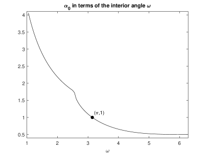
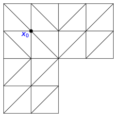
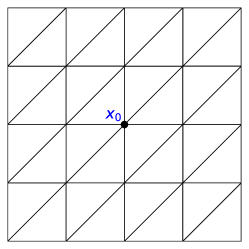
We sketch a drawing of the domain with a singular point in Figure 1. We assume the largest interior angle of the domain associated with the vertex . For simplicity of the analysis, we assume that
| (2.2) |
Let , satisfying be the solutions of the following characteristic equation
| (2.3) |
Then there exists a threshold
| (2.4) |
such that the following regularity result holds.
Lemma 2.2.
For any , let be the solution of the biharmonic problem (1.1). Then it follows with . Moreover, if , it holds ; and if , it holds .
The graph of in terms of the largest interior angle is shown in Figure 2, and some numerical values of are shown in Table 1 [29]. In 2.2, when , the regularity is dominated by the singularity of the Dirac delta source; and when , the regularity is dominated by the singularity of the domain [25, 5, 6, 18]. To design high-order accurate numerical methods, one has to handle the singularities introduced by these two singular sources: domain corner, and Dirac delta source.
| 4.0593 | 2.7396 | 2.0941 | 1.8854 | 1.5339 | 1.2006 | 0.7520 | 0.7178 | 0.6736 | 0.6157 | 0.5445 | 0.5050 |
2.2. interior penalty method
Let be a triangulation of domain satisfying . We denote the sets of interior and boundary edges of by and , respectively. We also set . We further denote the mesh size of by , and denote by . The length of an edge is denoted by . Here special attention has to be paid that the elements of are shape-regularity, it implies that mesh is locally quasi-uniform, i.e., if two elements and satisfy , there exists a constant such that,
| (2.5) |
Throughout the paper, we denote by one element such that the singular point , where is the closure of . If lies on an inner edge, either of the two triangles sharing that edge can be chosen as . Similarly, if is a vertex of several triangles, any one of these triangles can be chosen as . The diameter of is denoted by .
We define the broken Sobolev space associated with the triangulation by
The space equipped with the broken Sobolev norm and seminorm
The finite element space is
| (2.6) |
where is the space of polynomials of degree less than or equal to on element .
For each , we denote and by two adjacent triangles that share one common edge . The unit outward normal vector is oriented from to . We may designate as that with the higher of the indices. When , let be the element with the edge and denote by a unit outward normal vector to . For any , denote by and the two traces of along the edge . For a scalar function and a vector function that may be discontinuous across , we define the following jumps:
and averages
According to above definition, for and , it is clearly that
| (2.7) |
The following identity can be verified by simple algebraic manipulation
| (2.8) |
The interior penalty method for (1.1) is to find such that [32]
| (2.9) |
where the bilinear form
| (2.10) |
Here, the penalty parameter needs to be large enough to ensure the stability of the interior penalty method. Define the energy norm by
| (2.11) |
where
It can be observed that defines a norm on the space .
Recall that is defined in (2.1), we can observe that
| (2.12) |
The statement represents equivalence. Then the following inequalities hold.
2.3. A priori error estimate
Given the regularity outlined in 2.2, we review the following results, which are extensively used in the a priori and a posteriori error estimates.
Lemma 2.4 (Trace inequality [11]).
For any element and , it follows
Lemma 2.5 (Inverse inequality [11]).
For any element , , and , it follows
Lemma 2.6 (Interpolation error estimate [7]).
Let be the standard Lagrange nodal interpolation operator, then it follows
Based on the preparations above and the analysis in [8], the following a priori error estimate can be derived for the solution of the interior penalty method.
3. Residual-based a posteriori error estimators
To improve the convergence rate of the interior penalty method in 2.7, we propose an adaptive interior penalty method in this section. Specifically, we introduce two residual-type a posteriori error estimators for problem (1.1). Based on the derived error estimators and a bisection mesh refinement method, we then develop an adaptive interior penalty algorithm.
3.1. A posteriori error estimation based on primal problem
The first type of error estimator is obtained in a straightforward manner based on the problem (1.1). Theoretically, we establish upper and lower bounds to ensure the reliability and efficiency of the proposed estimator.
Let be the approximation solution obtained by the interior penalty method (2.9) for problem (1.1). For each , represents the set of three edges of element . Denote the set of all mesh nodes of the triangulation by . The number of nodes is equal to the degrees of freedom. For example, includes vertices and edge center points for the quadratic polynomial approximation. We propose the following residual-based a posteriori error estimator on involving the location of the Dirac point in the mesh
| (3.1) |
where
| (3.2) |
with for , for , and
| (3.3) | |||
| (3.4) |
Then the corresponding global error estimator is given by
| (3.5) |
If is not a vertex of the triangulation, an additional term appears in the indicators corresponding to the triangle .
To derive the reliability bound of a posteriori error estimator, we introduce the linear operator mapping elements in onto a conforming macro-elements space of degree . For the detailed definition of this conforming macro-elements, refer to [22, 16]. For the convenience of readers, we provide a brief review of the high-order versions of the classical Hsieh-Clough-Tocher macro-element.
Definition 3.1 ([22]).
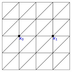
Let element . For , a macro-element of degree is a nodal finite element . Here, the element consists of subtriangles , satisfying as shown in Figure 3(a). The local element space on is defined by
| (3.6) |
The degrees of freedom on consist of all the following values:
-
•
The value and the first (partial) derivatives at the vertices of ;
-
•
The value at distinct points in the interior of each exterior edge of ;
-
•
The normal derivative at distinct points in the interior of each exterior edge of ;
-
•
The value and the first (partial) derivatives at the common vertex of all , where ;
-
•
The value and the normal derivative at distinct points in the interior of each edge of the , where , that is not an edge of ;
-
•
The value at distinct points in the interior of each chosen so that, if a polynomial of degree vanishes at those points, then it vanishes identically.
For example, the macro-element is a extension of the Lagrange element that consists of polynomials. These elements are illustrated in Figure 3, where we use the solid dot () to denote the value of the shape functions, the circle () to denote the value of all the first (partial) derivatives of the shape functions, and the arrow () to denote the value of the normal derivatives.
Denote by the set of elements containing a node , and let denote the number of elements in . We construct by averaging the nodal function values as follows:
| (3.7) |
Here, represents either the nodal value of a shape function, its first partial derivatives, or its normal derivative at , where is any node in the macro-elements space .
Lemma 3.1.
Remark 3.2.
We further introduce the following result.
Lemma 3.3 (Weak continuity).
Let be the solution of the problem (1.1). Then for any ,
| (3.9) | |||
| (3.10) | |||
| (3.11) | |||
| (3.12) |
Proof.
Given that , (3.9) and (3.10) follow immediately. We denote the set of the neighborhoods of the domain corners by and of the singular point by . Then . Therefore, (3.11) and (3.12) hold for any . To this end, we show that they also hold for . In the neighborhood of , the solution can be decomposed as , where and is the fundamental solution of the biharmonic equation with the Dirac delta function . It is straightforward to verify that (3.11) and (3.12) hold for any , and they can be similarly proved for any . ∎
Let be the collection of two adjacent elements that share the common edge . Specially, we define
For any , by (2.5) and the shape regular assumption, there exist positive constants and such that
Next, we are ready to present one of the main results.
Theorem 3.4 (Reliability).
Proof.
Let , the triangle inequality gives
| (3.14) |
By Lemma 3.1, it holds
To this end, it suffices to show that the second term on the right-hand side of (3.14) satisfies
| (3.15) |
By (2.12) and duality argument,
| (3.16) |
Denote the continuous interpolation polynomial of by . By (2.12), (2.1) and (2.9),
| (3.17) |
To estimate the first term on the right-hand side of (3.17), we consider the following three possibilities based on the different locations of . Recall that is the set of all mesh nodes of the triangulation.
(1) If , the values of and are equal at the node , i.e., , then
| (3.18) |
(2) If , but it is located inside one element , it follows
| (3.19) |
(3) If , but it belongs to an internal edge , then
| (3.20) |
According to the definition of and , it is clear that
Recall that . Then is continuous, and for any . By Lemma 3.3, it holds for any . Therefore,
which together with the integration by parts, and (2.8) yields
The sum of the two qualities above gives
Then, we estimate the five terms on the right hand side of the above equation one by one. Using the Cauchy-Schwarz inequality and Lemma 2.6 gives
| (3.22) |
| (3.23) |
and
| (3.24) |
For any , applying Lemma 2.6 and Lemma 2.5 gives
Recall that is equivalent to and . Summing up over all interior edges leads to
Similarly, for any , applying Lemma 2.6 and Lemma 2.5 gives
Then, by using the Cauchy-Schwarz inequality, it holds
| (3.25) |
| (3.26) |
∎
To prove the efficiency of the a posteriori error estimator, we will define four types of “bubble” functions and introduce some properties of these functions that are frequently used in error estimation and analysis. Let be a reference triangular or rectangular element. If is a triangle with the barycentric coordinates and , we denote the standard “bubble” function in by
| (3.27) |
If is a rectangle with the corresponding coordinates and , we denote the “bubble” function in by
| (3.28) |
For a triangle , we define as an affine element mapping, where is the reference triangle. Then the “bubble” function on is defined as
| (3.29) |
Lemma 3.5.
For the element “bubble” function on a triangle , it holds
| (3.30) |
Moreover, for , it follows
| (3.31) |
For each internal edge , let be the largest rhombus contained in that has as one of its diagonals. We define as an affine element mapping, where is the reference rectangle. The “bubble” function on element is defined by
| (3.32) |
where is the closure of .
Lemma 3.6.
For the “bubble” function in rhombus , it holds
| (3.33) | ||||
| (3.34) |
Moreover, for , it follows
| (3.35) |
Remark 3.7.
Inspired by the “bubble” functions in [20], where it is used to estimate the a posterior estimator of the discontinuous Galerkin method for the fourth-order elliptic problem with a source term in . Here we modify the definition of “bubble” functions and to accommodate two specific cases. Compared to [20], we further consider the effects of singularity point . As a result, the new “bubble” functions retain the favorable properties of the original ones and also obtain values of at , which is crucial for the subsequent proof of lower bounds.
Let be an affine function that satisfies and , where is the unit normal to the edge . Using the element “bubble” function definition given above, we define an edge “bubble” function as
| (3.36) |
Lemma 3.8.
For the edge “bubble” function in (3.36), it holds
| (3.37) | |||
| (3.38) | |||
| (3.39) |
Moreover, for , it follows
| (3.40) |
Denote by the collection of elements in that share a common edge or vertex with . Specially, we define the set
| (3.41) |
and the distance of to the boundary of is defined by . We define the smooth “bubble” function associated with the point by convolution of the characteristic function of the set satisfying
Lemma 3.9.
Assume that . For the “bubble” function , it holds,
| (3.42) | |||
| (3.43) |
Then we are ready to present our next main result.
Theorem 3.10 (Efficiency).
For the local indicator defined in (3.1), there exists a positive constant independent of the mesh size satisfying
| (3.44) |
Proof.
We first prove the estimate (3.44) on the element whose closure contains , but . By the definition of the energy norm, it holds
the estimation (3.44) is equivalent to
| (3.45) |
Then, we prove (3.45) in four steps.
(i) To prove . For , using integration by part gives
| (3.46) |
We set in (3.1), where and satisfies in . Additionally, is a polynomial on with . Then, for , it holds that . Consequently, (3.1) yields
According to Lemma 3.5, it holds
Then, by Cauchy-Schwarz inequality and Lemma 2.5,
| (3.47) |
Since is a piecewise polynomial over , according to (3.31) and (3.1), it holds
which implies
| (3.48) |
(ii) To prove . For , denote by . By (2.7), the summation of (3.1) over all elements gives
| (3.49) |
We take in (3.1), where is continuous on , and is a constant function in the normal direction to (i.e., ). By , Lemma 3.3, and Lemma 3.8, the equality (3.1) reduces to
By using Cauchy-Schwarz inequality and Lemma 2.5, the equation above gives
| (3.50) |
We extend from edge to by taking constants along the normal on . The resulting extension is a piecewise polynomial in . Setting , and using (3.35) and (3.40) yield
| (3.51) |
By (3.48), (3.1)-(3.1), it follows
which gives
| (3.52) |
Summing up (3.52) over all edges yields
| (3.53) |
(iii) To prove . We take in (3.1), where is continuous on and . By , 3.3, and 3.6, (3.1) can be written as
| (3.54) |
By (3.54), Cauchy-Schwarz inequality, and Lemma 2.5,
| (3.55) |
We extend to a function , defined over , by taking it to be constants along lines normal to . Setting and using (3.35) yield
| (3.56) |
| (3.57) |
Summing up (3.57) over all edges gives
| (3.58) |
(iv) To prove . By the weak formulation of (1.1) and Lemma 3.9, it can be observed
| (3.59) |
Let . By integration by parts, Cauchy-Schwarz inequality, Lemma 3.9 and Lemma 2.5,
| (3.60) |
Inserting (3.1) into (3.1) yields
| (3.61) |
which, together with (3.48), (3.53), and (3.58), implies
| (3.62) |
The estimate (3.45) follows from (3.48), (3.53), (3.58), and (3.62).
3.2. A posteriori error estimation based on regularized problem
Inspired by the technique of second-order elliptic equations with a Dirac delta source term, as discussed in [23], where the projection of the Dirac delta function is used to produce a regular solution, allowing adaptive procedures based on standard a posteriori error estimators to work efficiently. This regularization approach using projection techniques can also be applied for the problem (1.1).
More specifically, the Dirac delta function can be approximated by , defined as
where satisfying
Therefore, it holds
Let us consider the ensuing auxiliary problem:
| (3.64) |
The interior penalty method for problem (3.64) is to find such that
| (3.65) |
The well-posedness of the scheme (3.65) follows from the Lax-Milgram theorem. Let and be exact solutions for the original problem (1.1) and auxiliary problem (3.64), respectively. Let be corresponding numerical solutions of (3.65). The error estimate can be decomposed into two parts using the triangular inequality
| (3.66) |
The first term represents the regularization error, while the second term represents the discretization error. We estimate the total error by summing the independent contributions from each part.
Based on the regularity of the solution to (3.64), the discretization error can be estimated as [33, 8]
| (3.67) |
where with given in (2.4).
The error estimate (3.66) will be dominated by the regularization error. Referring to [33], the following projection error bound holds
| (3.68) |
where is the degree of the polynomial. Using the elliptic regularity theory and (3.68) yield
| (3.69) |
Lemma 3.11.
Remark 3.12.
Two techniques are empolyed in the interior penalty method to solve problem (1.1): a direct method (2.9) and a method using the projection technique (3.65). By comparing the error estimates of the solutions obtained with the direct method (see 2.7) and with the projection technique (see 3.11), we observe that solutions from both techniques exhibit the same convergence rate on quasi-uniform meshes.
Based on the projection technique, we propose the second residual-based a posteriori error estimator for the interior penalty method solving problem (1.1) as
| (3.70) |
the local indicator is given by
| (3.71) |
where
| (3.72) |
with for , for , and
The corresponding global upper and local lower bounds are given as follows.
Theorem 3.13 (Reliability).
Proof.
By triangular inequality, the left hand side of (3.73) is bounded from above by
Using the elliptic regularity bound, Lemma 3.3 and (3.69), the first term can be estimated as follows
| (3.74) |
Similar to the proof of Theorem 3.4, to prove , it is sufficient to verify that
| (3.75) |
where . Let be the continuous interpolation polynomial of . Then,
| (3.76) |
where
satisfies
| (3.77) |
By the Cauchy-Schwarz inequality and Lemma 2.6, the first term in (3.76) follows
| (3.78) |
which together with (3.74) and (3.77) yields the conclusion. ∎
Theorem 3.14 (Efficiency).
For the local indicator defined in (3.71), there exists a positive constant independent of the mesh size such that
| (3.79) |
Proof.
Let’s first show the element residual term satisfies the estimate (3.79). For , using integration by part gives
| (3.80) |
We set in (3.2), where and satisfies in . Noticing that . Consequently, (3.2) yields
By Lemma 3.5, it holds
We prove the first case in (3.79), i.e., . By Cauchy-Schwarz inequality, Lemma 2.5 and (3.69),
| (3.81) |
which implies
| (3.82) |
Note that for any . Similar to the proof of the first case in (3.79), it follows
| (3.83) |
Verifying other terms in can refer to the proof of Theorem 3.10. ∎
3.3. Adaptive finite element algorithm
The adaptive finite element algorithm based on the residual-based a posteriori error estimator (3.5) or (3.70) is summarized as follows.
Algorithm 1 The adaptive finite element algorithm.
4. Extensions
In this section, we extend our results to cover a broader class of fourth-order elliptic equations with various boundary conditions. Specifically, we generalize the biharmonic operator in (1.1) to a more general fourth order operator that includes low order terms
| (4.1) |
where (for ) are constants. Both residual-based a posteriori error estimators, (3.1) and (3.71), for problem (1.1) can be extended to the new operator. We only present the first type residual-based a posteriori error estimator for simplicity. The proofs of the efficiency and reliability are expected to be similar to those provided in Section 3. Therefore, we will focus solely on presenting the corresponding a posteriori error estimators and leave their performance to be verified numerically.
4.1. Non-homogeneous Dirichlet boundary conditions
Consider the following problem:
| (4.2) |
where and are given functions on the boundary , and is a given function in the domain . We assume that , , and are sufficiently smooth. This problem is a scalar analog of the variational problem for the strain gradient theory in elasticity and plasticity [35] when the coefficients satisfy and .
In [8], a interior penalty method was proposed to solve the general fourth-order elliptic equation without the Dirac delta function term . In the subsequent section, we extend and adapt this method to handle the presence of the Dirac delta function term on the right-hand side of equation (4.2).
We define the space associated with the triangulation by
| (4.3) |
Denote the subspace of by
| (4.4) |
where is a polynomial approximation function of by the interpolation on the boundary.
Unlike the interior penalty method for problems with homogeneous Dirichlet boundary conditions described in (2.9), the modified method (4.1) incorporates additional boundary term. These additional terms account for the non-homogeneous nature of the boundary conditions. The local error estimator on for interior penalty method (4.2) is given by
| (4.6) |
where
| (4.7) |
with , for , for , and
| (4.8) | |||
| (4.9) | |||
| (4.10) |
4.2. Navier boundary conditions
We also extend the results to the fourth order equation with Navier boundary conditions,
| (4.11) |
where and are given functions on the boundary , and is a given function within the domain . We also assume that , , and are sufficiently smooth. The problem (4.11) models a simply supported plate problem [34]. When the Dirac delta function term vanishes, [10] studied a symmetric interior penalty method for a fourth-order singular perturbation elliptic problem with these types of boundary conditions in two dimensions on polygonal domains. The interior penalty method for (4.11) is to find such that
| (4.12) |
where is defined as (2.6). The local error estimator for the interior penalty method (4.12) is given by
| (4.13) |
where
| (4.14) |
the element residual and the edge residuals , , are defined as (4.7). The boundary residual term is defined by
| (4.15) |
4.3. Homogeneous Neumann boundary conditions
For fourth-order elliptic equations with homogeneous Neumann boundary conditions, we consider the following model
| (4.16) |
where represent two distinct points strictly contained in the domain . These boundary-value problems can arise in the Cahn-Hilliard model, which describes phase-separation phenomena [14]. [9] proposed a quadratic interior penalty method for fourth-order boundary value problems with similar types of boundary conditions, assuming the right-hand side function . Under these conditions, a unique solution can be found, satisfying for .
It is straightforward to validate the solvability condition:
To obtain a unique solution, a common approach is to impose an additional constraint
We define a subspace of by
The finite element space associated with the triangulation is defined as
| (4.17) |
The interior penalty method for (4.16) is then to find such that
| (4.18) |
Note that the bilinear in (4.3) h is identical to that in (4.1), with the exception that the finite element space now includes only functions with a zero mean value.
5. Numerical examples
In this section, we present numerical test results to verify the accuracy of the interior penalty method and demonstrate the robustness of the proposed residual-type a posteriori estimators. If the exact solution is given, the convergence rate is calculated by
| (5.1) |
where is the finite element solution on the mesh obtained after th refinements of the initial triangulation . When the exact solution is unavailable or difficult to obtain, we instead use the following numerical convergence rate
| (5.2) |
Due to the lack of regularity, the interior penalty method with high-degree polynomial approximations on quasi-uniform triangular meshes may not achieve optimal convergence rates. To address this, we apply an adaptive interior penalty method to improve the convergence order.
The convergence rate of the a posteriori error estimator (resp. ) for polynomials with is quasi-optimal if
Here and in what follows, we abuse the notation to represent the total number of degrees of freedom.
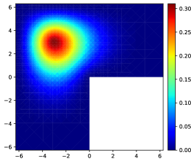
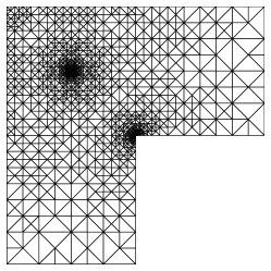
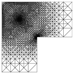
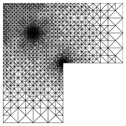
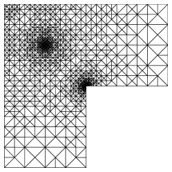
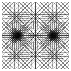
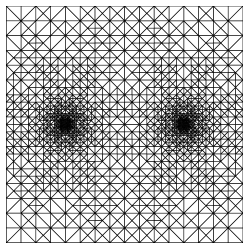
Example 5.1 (L-shape domain).
We consider problem (1.1) with homogeneous clamped boundary conditions in an L-shaped domain with a largest interior interior angle . The Dirac point , then the solution show singularities at two points and . We start with an initial mesh as Figure 4(a).
| j | 4 | 5 | 6 | 7 | 3 | 4 | 5 | 6 | 3 | 4 | 5 | 6 |
|---|---|---|---|---|---|---|---|---|---|---|---|---|
| 0.88 | 0.85 | 0.80 | 0.73 | 1.00 | 0.73 | 0.60 | 0.56 | 0.74 | 0.58 | 0.56 | 0.55 | |
Table 2 shows the convergence history using the -based interior penalty method on quasi-uniform meshes, with . From the results, we observe that the convergence rates are on coarse meshes, and on sufficiently refined meshes. This indicates that the singularity in the solution is primarily influenced by the reentrant corner of the polygonal domain when . The results in Table 2 align with the theoretical expectations outlined in Lemma 2.2.
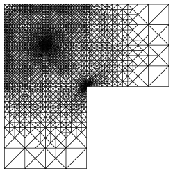
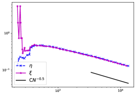
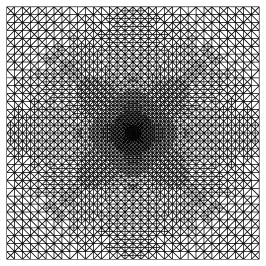
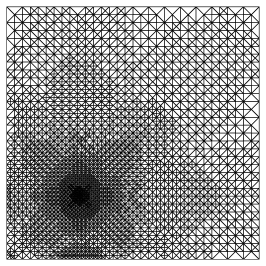
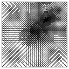
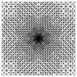
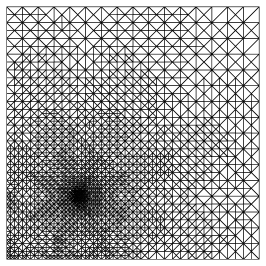
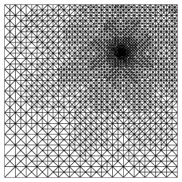
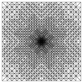
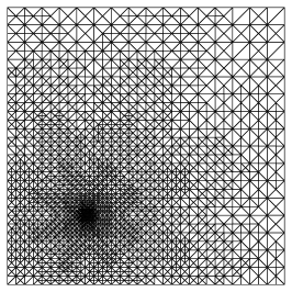
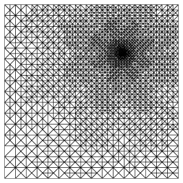
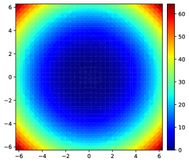
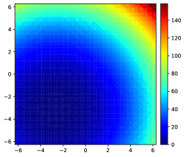
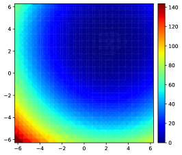
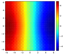
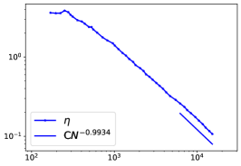
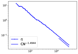
We then assess the efficiency of the a posteriori error estimators. Meshes generated by in (3.5) and in (3.70) are shown Figure 5 and Figure 6, respectively. It is evident that the error estimators effectively guide mesh refinements around the points and , where the solution shows singularities. As shown in Figure 7, the slopes for the estimators are close to when there are sufficient grid points, indicating optimal decay of the error with respect to the number of unknowns. The contours of the corresponding numerical solutions based on and are shown in Figure 4(b)-(c), they are very similar.


Example 5.2 (Non-homogeneous boundary).
In this example, we consider a more general biharmonic equation
| (5.3) |
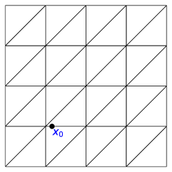
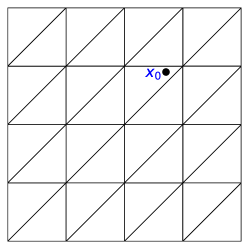
where the location of in are of three different types as shown in Case 1-3. The initial meshes of Cases 1-3 are reported in Figure 8.
-
Case 1:
is a node of the triangulations.
-
Case 2:
belongs to an inter edge .
-
Case 3:
is contained by one element .
We take the function
| (5.4) |
then the exact solution of equation (5.3) is given by
| (5.5) |
We consider (5.3) with two different boundary conditions and the parameters in are taken as .
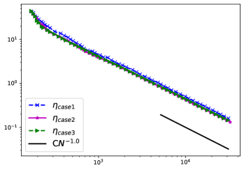
Test 1. We first consider non-homogeneous campled boundary conditions. The convergence rates of the interior penalty method solutions based on and polynomials for Case 1-3 in quasi-uniform meshes are shown in Table 3. The convergence rates are approximately . While the convergence rates for are quasi-optimal, the rates for only achieve suboptimal convergence. This is due to for . Given the low regularity of the solution , these results are the best that can be achieved with quasi-uniform meshes.
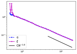
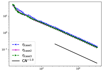
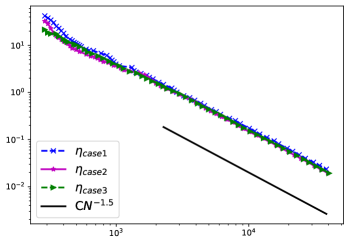
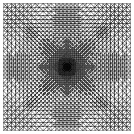
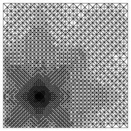
To address this, we apply the adaptive interior penalty method based on the residual-based a posteriori error estimator in (4.6). The corresponding numerical solutions of the adaptive algorithm using the error estimator are presented in Figure 11. Figure 9 and Figure 10 show the adaptive meshes of approximations, respectively. The error estimator effectively guides mesh refinements, particularly around the point . The convergence rates of the error estimator based on polynomials are illustrated in Figures 12(a)-(b), respectively. These results suggest that the convergence rates of are quasi-optimal for all three cases. Furthermore, with mesh refinement, the convergence slopes of the error estimators for Cases 1-3 nearly coincide. This demonstrates the superior performance of the adaptive algorithm based on the a posteriori error indicator presented in this work, especially when compared with uniform refinement.
Test 2. We set the non-homogeneous Navier boundary conditions. Similar to Test 1, we apply both the interior penalty method and the adaptive interior penalty method to this problem. Numerical results on uniform meshes are listed in Table 4. We perform and polynomial approximations using the adaptive interior penalty method, with the numerical results displayed in Figures 13-16. The results obtained are similar to those in Test 1. As mentioned earlier, (i) the convergence rates on uniform meshes are ; (ii) the position of the Dirac point within the cell has a negligible effect on the convergence rates, whether the meshes are adaptively refined or uniformly refined; (iii) refinements are concentrated around the point ; (iv) The convergence rates of are quasi-optimal.
| j | 4 | 5 | 6 | 7 | 3 | 4 | 5 | 6 | 2 | 3 | 4 | 5 |
|---|---|---|---|---|---|---|---|---|---|---|---|---|
| Case 1 | 0.99 | 0.99 | 1.00 | 1.00 | 1.60 | 1.41 | 1.18 | 1.06 | 1.97 | 1.59 | 1.14 | 1.02 |
| Case 2 | 0.98 | 0.99 | 0.99 | 1.00 | 1.67 | 1.72 | 1.20 | 0.96 | 1.72 | 1.59 | 1.35 | 0.87 |
| Case 3 | 0.98 | 0.99 | 0.99 | 1.00 | 1.68 | 1.72 | 1.33 | 1.23 | 1.93 | 1.60 | 1.32 | 0.94 |
| j | 4 | 5 | 6 | 7 | 3 | 4 | 5 | 6 | 2 | 3 | 4 | 5 |
|---|---|---|---|---|---|---|---|---|---|---|---|---|
| Case 1 | 0.99 | 0.99 | 1.00 | 1.00 | 1.60 | 1.41 | 1.18 | 1.06 | 1.97 | 1.59 | 1.14 | 1.02 |
| Case 2 | 0.98 | 1.00 | 0.99 | 1.00 | 1.67 | 1.72 | 1.19 | 0.95 | 1.68 | 1.57 | 1.35 | 0.87 |
| Case 3 | 0.99 | 0.99 | 0.99 | 1.00 | 1.71 | 1.75 | 1.33 | 1.23 | 1.94 | 1.58 | 1.32 | 0.94 |


Example 5.3 (Homogeneous Neumann boundary).
For the final example, we consider problem (4.16) with homogeneous Neumann boundary on convex domain . The right-hand side function is given as , where . An initial uniform triangular mesh is shown in Figure 17(a).
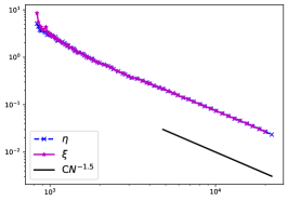
The convergence rates of the interior penalty method solutions based on polynomials on quasi-uniform meshes are shown in Table 5. We observe that . Due to the low global regularity of the solution, the convergence rates on quasi-uniform meshes can not reach the optimal order for polynomial approximations. For enhanced accuracy, the adaptive interior penalty method is better suited for this type of problem. The contour of adaptive interior penalty method approximation based on is shown in Figure 17(a). Figure 17(b)-(c) show the adaptive meshes of polynomial approximations, respectively. We can see clearly that the error estimator guides the mesh refinement densely around the points and . The convergence rates of error estimator based on polynomials are shown Figure 18(b)-(c). These results align with expectations, indicating that the convergence rates of the error estimator are quasi-optimal.
| j | 4 | 5 | 6 | 7 | 3 | 4 | 5 | 6 | 2 | 3 | 4 | 5 |
|---|---|---|---|---|---|---|---|---|---|---|---|---|
| 0.87 | 0.90 | 0.91 | 0.92 | 1.00 | 1.00 | 1.00 | 1.00 | 1.00 | 1.00 | 1.00 | 1.00 | |
6. Conclusion
Two residual-based a posteriori estimators are proposed for biharmonic problem (1.1). The first estimator is directly derived from the model equation, while the second estimator is based on the projection of the Dirac delta function onto the discrete finite element space. The later one introduces an additional projection error, which is included in the error estimator, yielding a similar effect to the first estimator in guiding mesh refinement. For both a posteriori estimators, we rigorously prove that these estimators are efficient and reliable. An adaptive interior penalty algorithm is provided based on the proposed a posteriori estimators. Extensions of the first estimator to more general fourth order elliptic equations are provided, and quasi-optimal convergence rates are numerically observed.
Acknowledgments
Y. Huang was supported in part by NSFC Project (12431014), Project of Scientific Research Fund of Hunan Provincial Science and Technology Department (2020ZYT003). N. Yi was supported by NSFC Project (12071400), Project of Scientific Research Fund of the Hunan Provincial Science and Technology Department (2024ZL5017), and Program for Science and Technology Innovative Research Team in Higher Educational Institutions of Hunan Province of China.
Data availability
Enquiries about data availability should be directed to the authors.
Declarations
The authors declare that they have no conflict of interest.
References
- [1] R. Araya, E. Behrens, and R. Rodríguez. A posteriori error estimates for elliptic problems with Dirac delta source terms. Numerische Mathematik, 105(2):193-216, 2006.
- [2] R. Araya, E. Behrens, and R. Rodríguez. An adaptive stabilized finite element scheme for a water quality model. Computer Methods in Applied Mechanics and Engineering, 196(29-30):2800-2812, 2007.
- [3] J.H. Argyris, I. Fried and D.W. Scharpf. The TUBA family of plate elements for the matrix displacement method. The Aeronautical Journal, 72(692):701-709, 1968.
- [4] J.P. Agnelli, E.M. Garau and P. Morin A posteriori error estimates for elliptic problems with Dirac measure terms in weighted spaces. ESAIM: Mathematical Modelling and Numerical Analysis, 48(6):1557-1581,2014.
- [5] C. Bacuta and J.H. Bramble and J.E. Pasciak. Shift theorems for the biharmonic Dirichlet problem. Springer: 1-26,2002.
- [6] M. Bourlard and M. Dauge and M.S. Lubuma and S. Nicaise. Coefficients of the singularities for elliptic boundary value problems on domains with conical points. III: Finite element methods on polygonal domains. SIAM Journal on Numerical Analysis, 29(1):136-155, 1992.
- [7] S.C. Brenner, T. Gudi, and L.Y. Sung. An a posteriori error estimator for a quadratic -interior penalty method for the biharmonic problem. IMA Journal of Numerical Analysis, 30: 777–798, 2010.
- [8] S.C. Brenner and L.Y. Sung. interior penalty methods for fourth order elliptic boundary value problems on polygonal domains. Journal of Scientific Computing, 23(23): 83-118, 2005.
- [9] S.C. Brenner, S. Gu, T. Gudi and L.Y. Sung. A quadratic interior penalty method for linear fourth order boundary value problems with boundary conditions of the Cahn–Hilliard type. SIAM Journal on Numerical Analysis, 50(4): 2088-2110, 2012.
- [10] S.C. Brenner and M. Neilan. A interior penalty method for a fourth order elliptic singular perturbation problem. SIAM Journal on Numerical Analysis, 49(2): 869-892, 2011.
- [11] S. Brenner and L. Scott. The mathematical theory of finite element methods. Volume 15 of Texts in Applied Mathematics, 3rd edn. Springer, New York, 2008.
- [12] C. V. Camp. A solution of the nonhomogeneous biharmonic equation by the boundary element method. Ph.D. thesis, Oklahoma State University, 1987.
- [13] Philippe G. Ciarlet. The Finite Element Method for Elliptic Problems. Université Pierre et Marie Curie, Paris, France, 1974.
- [14] J. W. Cahn and J. E. Hilliard. Free energy of a nonuniform system-I: Interfacial free energy. The Journal of Chemical Physics, 28(2): 258-267, 1958.
- [15] J.T. Chen, H. Z. Liao and W.M. Lee An analytical approach for the Green’s functions of biharmonic problems with circular and annular domains. Journal of Mechanics, 25(1): 59-74,2011.
- [16] J.J. Douglas, T. Dupont, P. Percell and R. Scott. A family of finite elements with optimal approximation properties for various Galerkin methods for 2nd and 4th order problems. RAIRO Analyse , 13(3):227–255, 1979.
- [17] G. Engel, K. Garikipati, T.J.R. Hughes, M.G. Larson, L. Mazzei and R.L. Taylor. Continuous/discontinuous finite element approximations of fourth-order elliptic problems in structural and continuum mechanics with applications to thin beams and plates, and strain gradient elasticity. Computer methods in applied mechanics and engineering, 191:3669-3750, 2002.
- [18] P. Grisvard. Singularities in Boundary Value Problems, volume 22 of Research Notes in Applied Mathematics. Springer-Verlag, New York, 1992.
- [19] W. Gong, M. Hinze and Z.J. Zhou. A priori error analysis for the finite element approximations of parabolic optimal control problems with pointwise control. SIAM Journal on Control and Optimization, 52(1):97-119, 2014.
- [20] E.H. Georgoulis, P. Houston and J. Virtanen. An aposteriori error indicator for discontinuous Galerkin approximations of fourth-order elliptic problems. IMA Journal of Numerical Analysis, 31:281-298, 2011.
- [21] F.D. Gaspoz, P.Morin and A, Veeser. A posteriori error estimates with point sources in fractional sobolev spaces . Numerical Methods for Partial Differential Equation, 33(4):1018-1042,2016.
- [22] E.H. Georgoulis, P. Houston and J. Virtanen. An a posteriori error indicator for discontinuous Galerkin approximations of fourth-order elliptic problems. IMA Journal of Numerical Analysis, 31(1): 281–298, 2009.
- [23] P. Houston and T. Wihler. Discontinuous Galerkin methods for problems with Dirac delta source. ESAIM: Mathematical Modelling and Numerical Analysis, 46(6):1467-1483, 2012.
- [24] J. D. Jackson. Classical electrodynamics. John Wiley and Sons, Inc., New York-London-Sydney, second edition, 1975.
- [25] V.A. Kozlov, V.G. Maza and J. Rossmann. Spectral problems associated with corner singularities of solutions to elliptic equations. American Mathematical Society, 85,2001.
- [26] S. B. G. Karakoc and M. Neilan. A finite element method for the Biharmonic problem without extrinsic penalization. Numerical Methods for Partial Differential Equations, 30(4),1254-1278,2014.
- [27] D. Leykekhman. Pointwise error estimates for interior penalty approximation of biharmonic problems. Mathematics of Computation, 90(327):41-63, 2020.
- [28] D. Leykekhman and B. Vexler. Optimal a priori error estimates of parabolic optimal control problems with pointwise control. SIAM Journal on Numerical Analysis, 51(5): 2797-2821, 2013.
- [29] H. Li, C. D. Wickramasinghe and P. Yin. A finite element method for the biharmonic problem with Dirichlet boundary conditions in a polygonal domain. arXiv preprint arXiv:2207.03838, 2022.
- [30] W. McLean. Strongly Elliptic Systems and Boundary Integral Equations. Cambridge University Press, 2000.
- [31] F. Millar, I.Muga, S Rojas and K.G. Van der Zee. Projection in negative norms and the regularization of rough linear functionals. Numerische Mathematik, 150: 1087-1121, 2022.
- [32] R. An and X.H. Huang. Constrained finite element methods for biharmonic problem. Abstract and Applied Analysis, 2012(137), 2012.
- [33] R. Scott. Finite element convergence for singular data. Numerische Mathematik, 21:317–327, 1973.
- [34] B. Semper. Conforming finite element approximations for a fourth-order singular perturbation problem. SIAM Journal on Numerical Analysis, 29(4): 1043-1058, 1992.
- [35] J.Y. Shu, W.E. King and N.A. Fleck. Finite elements for materials with strain gradient effects. International Journal for Numerical Methods in Engineering, 44(3): 373-391, 1999.
- [36] S. Timoshenko, S. Woinowsky-krieger. Theory of plates and shells. McGraw-hill New York, 1959.
- [37] F. Tan and Y. L. Zhang. The regular hybrid boundary node method in the bending analysis of thin plate structures subjected to a concentrated load. European Journal of Mechanics A/Solids, 38:79-89, 2013.