Marginal homogeneity tests with panel data††thanks: We thank seminar participants at Duke for helpful comments and discussion. Of course, all errors are our own.
Abstract
A panel dataset satisfies marginal homogeneity if the time-specific marginal distributions are homogeneous or time-invariant. Marginal homogeneity is relevant in economic settings such as dynamic discrete games. In this paper, we propose several tests for the hypothesis of marginal homogeneity and investigate their properties. We consider an asymptotic framework in which the number of individuals in the panel diverges, and the number of periods is fixed. We implement our tests by comparing a studentized or non-studentized -sample version of the Cramér-von Mises statistic with a suitable critical value. We propose three methods to construct the critical value: asymptotic approximations, the bootstrap, and time permutations. We show that the first two methods result in asymptotically exact hypothesis tests. The permutation test based on a non-studentized statistic is asymptotically exact when , but is asymptotically invalid when . In contrast, the permutation test based on a studentized statistic is always asymptotically exact. Finally, under a time-exchangeability assumption, the permutation test is exact in finite samples, both with and without studentization.
-
Keywords and phrases: Marginal homogeneity test, panel data, Cramér-von Mises statistic, Asymptotic approximation, Bootstrap, Permutation tests.
-
JEL classification: C12, C57, C63.
1 Introduction
This paper considers a hypothesis testing problem for panel data, . We assume that the data are independent and identically distributed (i.i.d.) across units , but allow for arbitrary dependence across time. For each period , let denote the common marginal cumulative distribution function (CDF) of . We say that the data generating process satisfies marginal homogeneity if these marginal distributions are homogeneous or time-invariant, i.e.,
| (1.1) |
In this paper, we propose several tests for the hypothesis of marginal homogeneity and investigate their properties.
Marginal homogeneity is relevant in economic models such as dynamic discrete games. In this case, researchers often observe , representing action and state variables for units (individuals, firms, etc.) over periods, respectively. In this context, a standard approach is to assume that the conditional choice probabilities (i.e., ) and state transition probabilities (i.e., ) are homogeneous, and posit a structural model for them. Under standard assumptions, these objects yield a homogeneous structural model for with parameter . This posited structure forms the basis of inference on in dynamic discrete choice games. Notably, this inference does not invoke the marginal homogeneity hypothesis in (1.1). However, if this condition holds, it provides valuable efficiency gains in the estimation of . To see this, note that marginal homogeneity in this context implies that is in a steady state with a marginal CDF , which yields the following structural equation:
| (1.2) |
Imposing (1.2) in the estimation of can deliver substantial efficiency gains relative to the standard method that does not impose it. In this sense, the marginal homogeneity hypothesis in (1.1) is a source of efficiency gains in the structural estimation of dynamic discrete choice games.
Beyond dynamic discrete games, marginal homogeneity tests have been applied to financial data. For example, Ditzhaus and Gaigall (2022) (see also references therein) tests for possible dependence between two stock market indices. In terms of our notation, we can express their data as , where represents the monthly returns of the first stock market (e.g., Nikkei 225 Stock Average) and represents the monthly returns of the second market (e.g., Dow Jones Industrial Average). Invoking classical models for stock prices, Ditzhaus and Gaigall (2022) posit monthly returns to be i.i.d. across (i.e., months), while the interconnectedness of global financial markets implies that there may be dependence across (i.e., stock markets). In this context, the marginal homogeneity hypothesis in (1.1) implies that the various stock markets have equally distributed returns. Finally, we note that their paper focuses on pairs of stock markets (i.e., ), whereas we consider applications with .
An inherent feature of the preceding examples is that the data are likely to exhibit dependence across time periods. In dynamic discrete games, actions and states depend on their past values. In fact, this is precisely what gives the discrete game its dynamic nature. In the application presented in Ditzhaus and Gaigall (2022), stock returns across the globe are likely to be interrelated. Beyond these two examples, dependence over time is common when dealing with panel data. For this reason, the classical goodness-of-fit testing literature focused on independent samples (e.g., Lehmann and Romano, 2022, Section 17.2.1), and its generalization to -sample problems, does not apply.
This paper studies the -sample testing problem with possibly dependent data. Namely, we implement our tests by comparing a studentized or non-studentized -sample version of the Cramér-von Mises statistic with a suitable critical value. We consider three possible methods to construct the critical value: asymptotic approximations, the bootstrap, and time permutations. We show that the first two methods lead to asymptotically exact hypothesis tests, with or without studentization. Results for the permutation test are more nuanced: the permutation test based on a non-studentized statistic is asymptotically exact when , but is asymptotically invalid when . Once studentized, the permutation test is always asymptotically exact. Finally, under a time-exchangeability assumption, the permutation test is exact in finite samples, both with or without studentization. On the other hand, relative to the non-studentized case, the asymptotic analysis of the studentized statistics requires an additional assumption: the variance-covariate matrix used in the studentization must be non-singular, an assumption that can fail in practice. See the related discussion in Section 2.2 and our empirical application in Section 6.
For independent cross-sectional data, the marginal homogeneity hypothesis in (1.1) becomes the standard equality-of-distribution hypothesis for -sample data, which has been thoroughly studied in the literature. In such case, Lehmann and Romano (2022, Theorem 17.2.1) shows that permutation tests of homogeneity are finite-sample exact. Chung and Romano (2013) explores the behavior of permutation tests with studentized test statistics. Relatedly, Bugni and Horowitz (2021) studies the application of permutation tests to functional cross-sectional data. Relatively speaking, the test for marginal homogeneity hypothesis in (1.1) with panel data (i.e., allowing for time dependence) has received less attention. Gaigall (2020) is among the first papers to test for marginal homogeneity in panel data with . In subsequent work, Ditzhaus and Gaigall (2022) broadened the analysis with to paired functional data. These papers show that permutation tests are asymptotically valid with two periods of panel data. Neither of these papers considers the case with , which is common in economic applications. To our knowledge, our paper is the first one to consider testing for marginal homogeneity in panel data models, allowing for . In this respect, one remarkable finding of our paper reveals that the asymptotic validity of the non-studentized permutation test breaks down when we consider .
A related testing problem in dynamic discrete choice games is concerned with evaluating the homogeneity of the state transition probabilities, i.e., for all . See Otsu et al. (2016) and Bugni et al. (2024) for recent contributions on this topic. The homogeneity of state transition probabilities and the marginal homogeneity in (1.1) are non-nested hypotheses, and so our contribution is complementary to but distinct from these references.
In other related work, Pauly et al. (2015) and Friedrich et al. (2017) investigate the validity of permutation tests to evaluate the presence of treatment effects in experiments under factorial designs. There are important differences between these papers and ours. The first key difference is in the class of data permutations used to implement the tests. Pauly et al. (2015) and Friedrich et al. (2017) generate their test by permuting observations in both units and time indices. In contrast, we generate our test by permuting the time index of our observations. We show that the classes of distributions under which the two types of permutation tests are finite-sample valid are non-nested; see Lemma A.2. Another difference is that Pauly et al. (2015) and Friedrich et al. (2017) focus on studentized statistics, while we consider both studentized and non-studentized statistics. In this respect, it is relevant to point out that analyzing studentized statistics requires additional assumptions compared to non-studentized ones; see discussion in Section 2.2. Finally, our Monte Carlo simulations suggest that our permutation test appears more powerful than theirs in finite samples. This is related to the fact that our permutation test only considers time index permutations, which provide a better contrast to detect departures from the marginal homogeneity hypothesis in (1.1).
The remainder of the paper is organized as follows. Section 2 introduces the hypothesis test problem in greater detail. Section 3 contains our main theoretical results. Section 4 discusses the power of the proposed inference methods. In Section 5, we evaluate the finite-sample performance of these tests via Monte Carlo simulations. Section 6 considers an empirical application based on Igami and Yang (2016). Section 7 concludes. The paper’s appendix collects all of the proofs and several auxiliary results.
2 The hypothesis testing problem
As the introduction explains, this paper considers a hypothesis-testing problem for panel data with units and time periods. Inspired by the typical application in economics, we consider an asymptotic framework in which grows and remains fixed. We denote the data by . As explained earlier, we allow the data to be arbitrarily dependent across time , and assume i.i.d. across units . We formalize this assumption next.
Assumption 1.
For all , are i.i.d. with marginal CDF .
Our goal is to test whether the marginal homogeneity hypothesis in (1.1) holds in the data, i.e.,
| (2.1) |
We propose implementing this hypothesis test by rejecting in (2.1) whenever a test statistic exceeds a suitable critical value. That is, for any significant level of , we propose
| (2.2) |
where indicates the test function, denotes the test statistic, and indicates the critical value. In the remainder of this section, we describe the test statistic (Section 2.1) and establish its asymptotic distribution under the null hypothesis of marginal homogeneity (Section 2.2). With these results in place, Section 3 provides three inference methods, each based on a different type of critical values.
2.1 Test statistics
We propose implementing our test using the Cramér-von Mises (CvM) statistic, given by the sample-weighted sum of squared differences of the empirical CDFs for all consecutive periods. For simplicity, we evaluate these differences on a finite number of user-defined points on the real line with . For reasons that will be explained soon, we refer to this as the non-studentized CvM statistic, given by
| (2.3) |
where is the empirical CDF in period , and is the empirical analog of the aggregate probability in the interval , i.e., ,
| (2.4) |
It is easy to see that (2.3) can be reexpressed as follows
where and, for all ,
| (2.5) |
Under in (2.1), our formal arguments (see the proof of Theorem 2.1) reveal that is asymptotically distributed according to , where for each ,
| (2.6) | ||||
and is the aggregate probability in the interval ,
| (2.7) |
As a corollary, has a generalized chi-squared asymptotic distribution under in (2.1), with weights determined by the eigenvalues of . The dependence of the limiting distribution on explains why we refer to as the non-studentized CvM statistic.
If is a non-singular matrix, it is natural to also consider a studentized version of the CvM statistic. To this end, we consider the studentized CvM statistic, given by
| (2.8) |
where is the generalized inverse of the empirical analog of , denoted by . For each , we define as follows:
| (2.9) | ||||
for each . If in (2.1) holds and is a non-singular, has a chi-squared asymptotic distribution with degrees of freedom. The lack of dependence of this limiting distribution on justifies referring to as the studentized CvM statistic.
Remark 2.1 (On the choice of test-statistics).
The test statistics in (2.3) and (2.8) are CvM-type statistics evaluated over a finite set of points . In principle, our analysis extends to other types of test statistics evaluated over these points, such as the Kolmogorov-Smirnov statistic. It is also worth reiterating that can be arbitrarily chosen by the researcher. In this respect, the most important simplifying aspect in (2.3) and (2.8) is that we use a finite number of points rather than an infinite number of points, such as a continuum.
There are several reasons to prefer a finite set over a continuum. First and foremost, it leads to simpler asymptotic analysis regarding the studentization of test statistics. Second, for applications in which the data are discrete and with finite support , one can set without any loss of information (note that equality of marginal distributions for all points in is equivalent to ). Many empirical applications, including the one in Section 6, feature discrete data with finite support. Third, the extension to the continuum case could be implemented along the lines of the Khmaladze (2016) transformation. See also the related work by Chung and Olivares (2021). Having said this, this extension requires new and considerably more complicated arguments, which we consider out of the scope of our paper.
2.2 Asymptotic distribution under the null hypothesis
In this section, we derive the asymptotic distribution of the non-studentized CvM statistic in (2.3) and the studentized version in (2.8). Our characterization of the asymptotic distribution of the studentized CvM statistic relies on the following assumption.
Assumption 2.
is positive definite.
We note that Assumption 2 is required for our asymptotic analysis of the studentized CvM statistic and is not necessary in the case of the non-studentized version. For a suitable choice of , Assumption 2 is widely applicable to many data-generating processes. We now describe scenarios in which this assumption does not hold. First, note that Assumption 2 would fail if includes any point that is “irrelevant” with respect to the support of , i.e., for some . An example of this occurs for any that lies below the support of . In this case, one can always restore the validity of Assumption 2 by removing all of these irrelevant points. Second, one should never include that equals or exceeds the support of . Doing this would result in , leading to , rendering singular. Finally, would be singular if there is no full communication between some states. For example, consider a Markov chain for with for all , where for any ,
This transition matrix implies no communication between the first and last two states. Then, for any , producing a singular .
The next result establishes the asymptotic distribution of the non-studentized and studentized CvM statistics under the marginal homogeneity hypothesis in (2.1).
Theorem 2.1.
Theorem 2.1 shows that under the marginal homogeneity hypothesis, the non-studentized CvM statistic in (2.3) converges to a generalized chi-square distribution with the weights determined by the eigenvalues of . Since is not necessarily positive definite, some eigenvalues may be zero, leading to reduced degrees of freedom. When is positive definite, then the limiting distribution of studentized CvM statistic in (2.8) is chi-square distributed. These results are the basis of the critical values proposed in the following section.
3 Critical values and validity of inference
This section describes three critical values for the CvM test statistics proposed in Section 2.1. Each critical value gives rise to a different hypothesis test according to equation (2.2). We formally study the validity of each one of these methods.
3.1 Asymptotic approximation
In this section, we propose a hypothesis test for (2.1) by approximating the quantiles of the asymptotic distribution in Theorem 2.1. To this end, we now introduce some notations. For any , let denote a random variable with the generalized chi-square distribution of weights equal to , unit vector of degrees of freedom, zero vector of non-centrality parameters, and no constant or normal terms. Also, for any , let denote the CDF of evaluated at . This function can be numerically computed with arbitrary accuracy by simulating its empirical distribution.
For the non-studentized CvM statistic, we propose
| (3.1) |
where denotes the eigenvalues of , and the following hypothesis test:
| (3.2) |
For the studentized CvM statistic, we propose the following hypothesis test:
| (3.3) |
where equals the -quantile of the (standard) chi-squared distribution with degrees of freedom.
3.2 Bootstrap
This section proposes a hypothesis test for (2.1) via the bootstrap. To this end, we repeatedly resample the data with replacement across units to construct a bootstrap sample, denoted by . For each bootstrap sample, the bootstrap analog of the non-studentized and studentized CvM statistics are given by
| (3.4) |
where, for all ,
| (3.5) |
Remark 3.1.
One could also define in (3.4) with replaced by its bootstrap analog. Our main text omits this option for brevity, but we include it in our Monte Carlo simulations.
By repeating the bootstrap sampling sufficiently many times, we can approximate the conditional distributions and with arbitrary accuracy.
For the non-studentized CvM statistic, we propose
| (3.6) |
and the following hypothesis test:
| (3.7) |
For the studentized CvM statistic, we propose
| (3.8) |
and the following hypothesis test:
| (3.9) |
3.3 Permutations
In this section, we propose a hypothesis test for (2.1) by random permutations of the data. Our permutations are motivated by the marginal homogeneity hypothesis in (1.1), and they consist of randomly permuting the time index for each unit .
These tests require the following notation. Let denote the set of all permutations of the indices , and is defined as the set of all possible permutations of the time indices over observations. A typical element of is given by , where denotes the permuted time index of the observation , and is an arbitrary time permutation that belongs to the set . In other words, the permuted version of the data can be written as .
For each permutation , the permutation analog of the non-studentized and studentized CvM statistics are given by
| (3.10) |
where, for all ,
| (3.11) |
and, for all ,
| (3.12) | ||||
where and .
These permutation test statistics can be used to construct permutation-based tests along the lines of Lehmann and Romano (2022, Section 17.2.1). For the non-studentized CvM statistic, we propose a critical value , which is the -quantile over all possible permutations of the non-studentized CvM statistics (denoted by ). The corresponding hypothesis test is defined as:
| (3.13) |
For the studentized CvM statistic, we propose the analogous object but for the studentized CvM statistic. That is, equals to the -quantile over all the possible permutations for the studentized CvM statistics (given by ). The corresponding hypothesis test is given by:
| (3.14) |
Remark 3.2.
The tests in (3.13) and (3.14) are the non-random versions of the standard permutation tests described in Lehmann and Romano (2022, Section 17.2.1). The key difference between the non-random and the random versions lies in the handling of ties between the test statistic and the critical value: the non-random version does not reject, while the random version rejects with a specific probability. While being more conservative, the non-random version is preferred because it involves a simpler decision rule similar to the one used in previous tests.
Theorem 3.3.
We first describe the result for the non-studentized test in (3.13). Part (a) shows that the non-studentized test is asymptotically valid for . This result aligns with the analysis in Gaigall (2020) and Ditzhaus and Gaigall (2022). Part (b) reveals that the previous result fails for . This finding is apparently new in the literature and empirically relevant, as many economic applications involve panel data with more than two periods. To gain intuition about (a) and (b), it is useful to compare the variance-covariance of the th observation, i.e., , before and after permutations. If the variance-covariance remains the same, then the permutation test can be shown to be asymptotically valid. See the proof of Theorem 3.3 for a formal justification. When , the th observation is before the permutation and a mixture of and after the permutation. Under in (2.1), these two random vectors share the same variance-covariance matrix. When , this equivalence breaks down. For example, when , the th observation is before the permutation and a mixture of , , , , , and after the permutation. The variance-covariance matrix of the former and the latter differ even under in (2.1).
Finally, part (c) of Theorem 3.3 shows that the studentized test in (3.14) is asymptotically valid for any . This result is in line with several studies in the literature that prove the asymptotic validity of permutation tests for suitably normalized test statistics, e.g., Janssen (1997); Chung and Romano (2013); DiCiccio and Romano (2017); Chung and Olivares (2021). This result is also related to the earlier discussion regarding variance-covariance matrices of the th observation before and after permutations. Once the data is studentized, the variance-covariance matrix of the th observation is asymptotically invariant to permutations. By the previous paragraph’s logic, the permutation test is asymptotically valid for the studentized test statistic.
An important advantage of the permutation tests over the ones described in previous subsections lies in their finite-sample validity under an important class of distributions that satisfy in (2.1). To explain this clearly, let denote the set of distributions that satisfy time exchangeability, i.e., for any , has the same distribution as for each . The next result describes the finite-sample validity of our test under suitable conditions.
Theorem 3.4.
Theorem 3.4 implies that our permutation tests are finite-sample valid under suitable conditions. Part (a) says that a time-exchangeable distribution satisfies the null hypothesis in (2.1) under our maintained Assumption 1. Under such distribution, the permutation tests provide finite-sample size control. We stress that size control is not exact (i.e., the inequalities in (3.15) might be strict) only because we are using a non-randomized permutation test; see Remark 3.2. That is, if we replaced our permutation test with its random version, these would enjoy exact size control (i.e., both inequalities in (3.15) would hold with equality).
The combination of Theorems 3.3 and 3.4 justifies the use of studentized permutation test in (3.14) (and also the non-studentized one in (3.13) when ). Theorem 3.3 indicates that this test is asymptotically exact, and Theorem 3.4 shows that it is finite-sample valid for an important class of distributions in . As already mentioned, the finite-sample validity makes the permutation test an exceptionally attractive inference method compared to those discussed in previous subsections.
Remark 3.3.
It is worth noting that our class of time permutations differs from the class of “all permutations” that uniformly permute both time periods and units. The latter has been used in the previous literature, such as Friedrich et al. (2017). Naturally, our time permutations form a strict subset of the class of “all permutations”. On the flip side, under our maintained Assumption 1, the class of distributions that satisfy exchangeability over “all permutations” is more restrictive than the set of distributions that satisfy time exchangeability only; see Lemma A.2. In other words, if we used a permutation test based on “all permutations”, we could only demonstrate Theorem 3.4 for a substantially smaller class of distributions than .
4 Power analysis
This section briefly describes the power properties of the various hypothesis-testing procedures considered in this paper. Given the results in Section 3, we restrict attention to the hypothesis tests that are asymptotically valid under Assumptions 1–2:
-
•
The asymptotic approximation-based test, both non-studentized and studentized.
-
•
The bootstrap-based test, both non-studentized and studentized.
-
•
The studentized permutation-based test.
-
•
The non-studentized permutation-based test for .
As explained in Section 2.1, our CvM test statistic is defined to detect differences in marginal CDFs at any point in . We thus focus our power analysis on the following subset of :
| (4.1) |
For all fixed hypotheses in , it is not hard to see that the CvM test statistic in (2.3) and (2.8) diverges. At the same time, one can establish that the critical values described throughout this paper remain bounded in probability. For this reason, all asymptotically valid tests are consistent against any fixed hypothesis in .
We now compare the local power properties of these tests. We consider local alternative hypotheses under , which are sequences of DGPs whose marginal CDFs satisfy with . Under these sequences of distributions, we can repeat the arguments used to prove Theorem 2.1 to establish the asymptotic distribution of the CvM test statistic in (2.3) and (2.8). It is not hard to see that these become the non-central versions of the asymptotic distributions in (2.10) and (2.11) under . Moreover, under these local alternatives, the critical values considered throughout this paper can be shown not to change their asymptotic behavior. As a corollary, the asymptotically valid tests based on the non-studentized statistics share the same local power properties, and the same holds for the asymptotically valid tests based on the studentized statistics.
5 Monte Carlo simulations
This section investigates the finite-sample performance of the various tests for marginal homogeneity tests proposed in this paper. To this end, we repeatedly simulate independent panel datasets where, for each and ,
with
where is a sequence of constants and is a constant positive-definite matrix. By definition, is a random effect and are transient shocks with variance-covariate matrix . We consider two specifications for :
-
•
WN: , i.e., is a white noise process with zero mean and unit variance. The distribution of is time-exchangeable under this specification.
-
•
AR(1): for all with , and , i.e., is an AR(1) process zero mean, variance one, and correlation coefficient . In this case, the distribution of is not time-exchangeable.
We consider two options for , which determines whether the data satisfies marginal homogeneity or not. For simulations under in (2.1), we use for . For simulations under in (2.1), we set for .
To compute the CvM statistics we set equal to the 1/6, 2/6, 3/6, 4/6, and 5/6 empirical quantiles of (thus, ). For each dataset, we implemented the following tests with a significance level of :
We consider simulations with units and periods. The results shown in the tables are obtained from independent panel data draws based on the design described.
Table 1 describes the rejection rates of the various tests under marginal homogeneity, i.e., in (2.1). When , all our proposed hypothesis tests (AA, BS, PT, studentized or not) provide exact size control when is sufficiently large. These results are consistent with our asymptotic analysis. This conclusion also seems to apply to the BS2 and the studentized PT2 tests. On the other hand, the non-studentized PT2 test does not control size. This is consistent with our discussion in Lemma A.2, where we argue that the permutation class used to implement our PT tests is qualitatively different from the one used for the PT2 tests. Our simulations also allow us to examine how our asymptotically valid methods perform when is relatively small. In this respect, one interesting finding is that the non-studentized versions of the AA and BS tests outperform their corresponding studentized ones when is small. On the other hand, the PT test performs equally well with and without studentization for small . The results for are qualitatively similar to those for , except for the PT test. For , our formal results show that the studentized PT test is asymptotically valid, but the non-studentized PT test is not. This is clearly evidenced in our simulations with AR(1) shocks, where the non-studentized PT test exhibits rejection rates close to 13%. However, if data is time-exchangeable as with the WN shocks, then we observe that PT test is finite-sample valid regardless of studentization even if .
| Test type | Critical value | |||||||
|---|---|---|---|---|---|---|---|---|
| WN | Non-stud. | AA | 5.48 | 5.54 | 5.08 | 4.76 | 5.16 | |
| BS | 5.60 | 5.36 | 5.14 | 4.78 | 5.06 | |||
| PT | 4.54 | 4.94 | 4.82 | 4.62 | 5.08 | |||
| PT2 | 1.02 | 0.80 | 0.76 | 0.96 | 1.00 | |||
| Studentized | AA | 14.34 | 8.54 | 6.94 | 6.08 | 4.96 | ||
| BS | 14.24 | 8.56 | 6.98 | 6.00 | 4.86 | |||
| BS2 | 2.56 | 4.66 | 5.02 | 5.30 | 4.54 | |||
| PT | 5.06 | 5.08 | 5.20 | 5.20 | 4.44 | |||
| PT2 | 4.50 | 5.02 | 5.16 | 5.28 | 4.44 | |||
| AR(1) | Non-stud. | AA | 5.12 | 6.02 | 5.12 | 5.24 | 5.22 | |
| BS | 5.36 | 5.90 | 5.12 | 5.22 | 5.10 | |||
| PT | 4.16 | 5.32 | 4.88 | 5.00 | 5.06 | |||
| PT2 | 3.46 | 4.58 | 4.32 | 4.62 | 4.54 | |||
| Studentized | AA | 14.00 | 8.78 | 6.88 | 6.30 | 5.58 | ||
| BS | 14.18 | 8.96 | 6.98 | 6.40 | 5.52 | |||
| BS2 | 3.58 | 4.86 | 5.16 | 5.38 | 5.08 | |||
| PT | 5.12 | 5.36 | 5.16 | 5.34 | 5.00 | |||
| PT2 | 5.10 | 5.32 | 5.40 | 5.42 | 5.16 | |||
| WN | Non-stud. | AA | 5.68 | 4.80 | 5.46 | 5.16 | 5.56 | |
| BS | 5.84 | 4.74 | 5.38 | 5.22 | 5.52 | |||
| PT | 5.30 | 4.66 | 5.38 | 5.00 | 5.38 | |||
| PT2 | 0.88 | 0.72 | 0.60 | 0.94 | 1.10 | |||
| Studentized | AA | 35.82 | 16.74 | 9.88 | 7.04 | 5.80 | ||
| BS | 36.00 | 16.78 | 9.90 | 6.98 | 5.84 | |||
| BS2 | 0.70 | 3.28 | 4.66 | 4.82 | 4.92 | |||
| PT | 5.02 | 5.08 | 4.98 | 4.84 | 4.88 | |||
| PT2 | 3.78 | 4.52 | 4.82 | 4.66 | 4.86 | |||
| AR(1) | Non-stud. | AA | 6.22 | 6.18 | 5.76 | 5.20 | 5.64 | |
| BS | 6.08 | 6.24 | 5.74 | 5.42 | 5.38 | |||
| PT | 12.70 | 13.80 | 13.88 | 13.68 | 12.96 | |||
| PT2 | 6.14 | 7.30 | 6.94 | 6.44 | 6.84 | |||
| Studentized | AA | 33.44 | 17.06 | 10.38 | 7.26 | 5.96 | ||
| BS | 33.94 | 16.92 | 10.12 | 7.22 | 5.80 | |||
| BS2 | 1.78 | 3.14 | 4.26 | 4.80 | 4.98 | |||
| PT | 4.62 | 5.26 | 5.08 | 5.14 | 5.12 | |||
| PT2 | 3.36 | 4.54 | 4.84 | 4.86 | 5.02 |
Table 2 explores the performance of the same test for data configurations that do not satisfy marginal homogeneity. To make the comparison fair, we focus on asymptotically valid inference methods. For , this includes studentized and non-studentized versions of the AA, BS, and PT tests, and studentized BS2. Our results indicate that studentized tests are considerably more powerful than their corresponding non-studentized versions. The main difference in the case of , is that we now have to eliminate the non-studentized PT test. With this exception, the results with are qualitatively similar to those for .
| Test type | Critical value | |||||||
|---|---|---|---|---|---|---|---|---|
| WN | Non-stud. | AA | 8.04 | 11.06 | 16.22 | 32.12 | 65.34 | |
| BS | 8.06 | 11.00 | 16.34 | 32.12 | 65.08 | |||
| PT | 6.66 | 10.20 | 15.78 | 31.68 | 64.98 | |||
| PT2 | 1.30 | 2.14 | 3.44 | 7.64 | 28.86 | |||
| Studentized | AA | 19.88 | 18.74 | 27.12 | 46.40 | 78.66 | ||
| BS | 20.04 | 18.70 | 27.14 | 46.50 | 78.86 | |||
| BS2 | 4.92 | 10.96 | 22.38 | 43.90 | 77.68 | |||
| PT | 8.32 | 11.96 | 22.60 | 43.94 | 77.72 | |||
| PT2 | 7.66 | 11.74 | 22.42 | 43.82 | 77.84 | |||
| AR(1) | Non-stud. | AA | 6.50 | 7.64 | 9.54 | 18.14 | 39.56 | |
| BS | 6.58 | 7.76 | 9.22 | 18.14 | 39.70 | |||
| PT | 5.36 | 7.08 | 8.90 | 17.80 | 39.40 | |||
| PT2 | 4.48 | 6.10 | 7.90 | 15.68 | 36.88 | |||
| Studentized | AA | 18.82 | 17.60 | 22.52 | 40.96 | 72.34 | ||
| BS | 18.96 | 17.76 | 22.50 | 40.90 | 72.24 | |||
| BS2 | 5.16 | 10.96 | 18.26 | 38.30 | 71.30 | |||
| PT | 7.48 | 11.48 | 18.48 | 38.36 | 71.06 | |||
| PT2 | 7.46 | 11.52 | 18.52 | 38.44 | 71.22 | |||
| WN | Non-stud. | AA | 6.98 | 8.50 | 12.70 | 27.70 | 72.42 | |
| BS | 7.16 | 8.54 | 12.64 | 27.78 | 72.56 | |||
| PT | 6.32 | 8.14 | 12.18 | 27.26 | 72.44 | |||
| PT2 | 1.00 | 1.34 | 1.58 | 3.78 | 18.86 | |||
| Studentized | AA | 51.14 | 46.10 | 62.68 | 89.28 | 99.66 | ||
| BS | 51.22 | 45.94 | 62.56 | 89.20 | 99.68 | |||
| BS2 | 1.86 | 16.14 | 47.42 | 85.40 | 99.60 | |||
| PT | 11.30 | 21.28 | 48.82 | 85.74 | 99.60 | |||
| PT2 | 9.20 | 19.60 | 47.88 | 85.52 | 99.54 | |||
| AR(1) | Non-stud. | AA | 6.38 | 7.16 | 7.56 | 10.44 | 21.30 | |
| BS | 6.34 | 7.10 | 7.64 | 10.58 | 21.28 | |||
| PT | 14.26 | 16.64 | 19.74 | 28.10 | 65.38 | |||
| PT2 | 6.42 | 8.42 | 9.38 | 12.98 | 28.18 | |||
| Studentized | AA | 62.84 | 72.54 | 94.60 | 99.94 | 100.00 | ||
| BS | 63.34 | 72.50 | 94.60 | 99.94 | 100.00 | |||
| BS2 | 6.24 | 33.40 | 86.92 | 99.88 | 100.00 | |||
| PT | 16.30 | 45.90 | 89.34 | 99.88 | 100.00 | |||
| PT2 | 13.00 | 43.08 | 88.52 | 99.88 | 100.00 |
Tables 1 and 2 offer interesting conclusions regarding the finite sample properties of the asymptotically valid tests. When the sample size is relatively small, the non-studentized tests appear to provide better size control than their studentized counterparts, though at the expense of lower power. As the sample size increases, the studentized tests improve their size control. As a result, the studentized tests seem to be a better option for larger sample sizes: they offer adequate size control and relatively higher power compared to their non-studentized versions.
6 Empirical application
This section applies our marginal homogeneity tests to the state variable in the dynamic discrete choice game in Igami and Yang (2016). In this paper, the authors develop and estimate a dynamic entry model oligopoly game among Canada’s five main hamburger chains: A&W, Burger King, Harvey’s, McDonald’s, and Wendy’s. They use yearly data from 400 geographical markets111The paper defines a market as a cluster of stores located within a 0.5-mile radius at any point of their sample period. Markets in downtown areas are omitted as these experience a different nature of competition. located in seven major Canadian cities between 1970 and 2004, i.e., and . For each market-year pair , they observe the number of stores for each chain, population, and income.
The state variable used in Igami and Yang (2016) is a discrete categorical variable whose value represents the number of stores of each chain, population, and income of a given market-year pair. We now briefly explain its construction, and defer to their Igami and Yang (2016, Section 4.1) for details. The paper restricts the number of stores per chain to three, and divides population and income into quartiles.
For each period and market , is uniquely determined by the number of stores (up to three) for each chain , , the population quartile , and the income quartile . So, indicates that for all , , and , indicates that for all , , and , and so on, until indicates that for all , , and . While could take up to possible values, it only takes distinct values in the entire dataset.
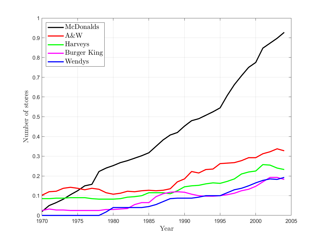
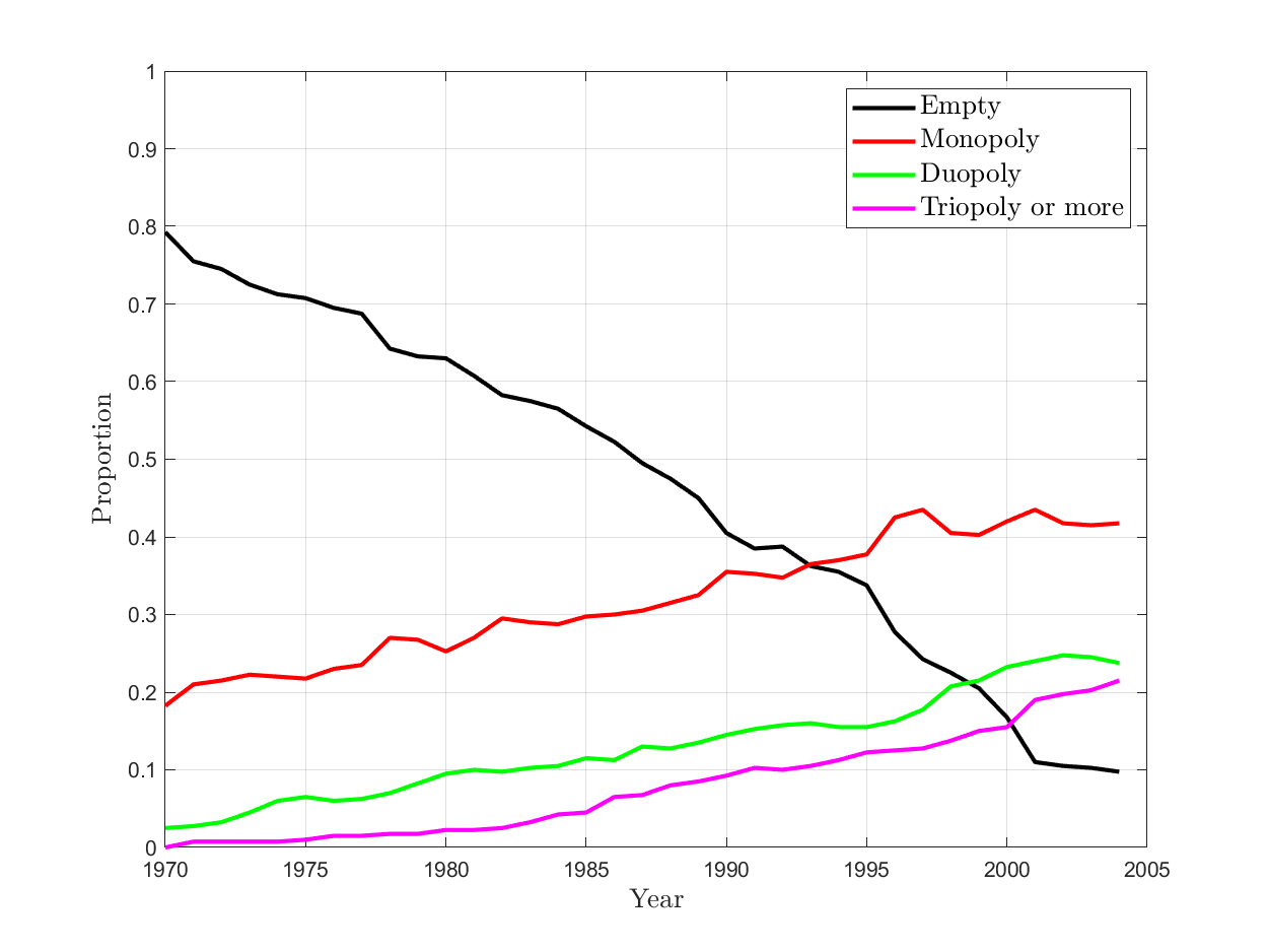
The data spans an extensive period in which the Canadian fast-food industry grew considerably. As Igami and Yang (2016, Section 3.2) reports, the average number of shops per market was less than 0.5 during 1970’s to approximately 1.8 in the early 2000’s. We now provide further evidence about the evolution of this industry. Figure 1 shows the average number of stores per market over time desegregated by chain. This figure shows that the average number of stores per market has increased across all chains, with the most significant increase observed for McDonald’s compared to the other chains. Figure 2 shows the average number of competitors per market over time. This figure reveals that the frequency of empty markets decreased steadily between 1970 and 2000, while the frequencies of monopoly, duopoly, and triopoly or more steadily increased over the same period. In contrast, during 2000-2004, the frequency of each market type has remained relatively stable. This evidence suggests that the Canadian fast-food industry has been evolving between 1970 and the early 2000’s, and may have reached a steady state during the last years of the sample. The hypothesis tests developed in this paper can be used to evaluate whether the state distribution is homogeneous over any of the periods in the sample.
As explained in Section 1, the marginal homogeneity of the state variable can be a source for efficiency gains in the estimation of dynamic discrete games. With this motivation in mind, we now apply our marginal homogeneity tests to our panel data of the state variable. Given the large number of values that the variable takes, Assumption 2 does not hold over the sample period. For this reason, we only consider non-studentized tests. We implement our tests for two subsets of periods. Since we consider panel data with , the non-studentized asymptotic approximation and bootstrap tests are valid, but the permutation test is not. Table 3 presents the results of our hypothesis tests for two subsets of sample periods. First, we consider a subset of our data every five years, i.e., 1970, 1975, 1980, 1985, 1990, 1995, and 2000. In this case, our tests strongly reject the hypothesis of marginal homogeneity. This result is expected, as it is consistent with the informal discussion in the previous paragraph regarding the growth of the Canadian fast-food industry between 1970 and 2000. Second, we repeat the analysis for the last four years in the sample period, i.e., 2001, 2002, 2003, and 2004. In this case, our tests do not reject the hypothesis of marginal homogeneity. These results suggest that the Canadian fast-food industry may be in a steady state in the latter part of the sample period.
| Sample | Test type | Test statistic | Critical Value with | ||
|---|---|---|---|---|---|
| Asy. approx. | Bootstrap | Permutation | |||
| Pre-2000 | Non-stud. | 10.76 | 0.88 | 0.82 | 2.35 |
| Post-2000 | Non-stud. | 0.08 | 0.13 | 0.13 | 0.23 |
7 Conclusions
This paper proposes hypothesis tests to evaluate whether panel data satisfies the hypothesis of marginal homogeneity. As we argue in the paper, marginal homogeneity is a relevant property in economic settings such as dynamic discrete games.
Our asymptotic framework for panel data considers a diverging number of units and a fixed number of periods . We implement our tests by comparing a studentized or non-studentized -sample version of the Cramér-von Mises statistic with a suitable critical value. Relative to the non-studentized case, the asymptotic analysis of the studentized statistics requires an additional assumption: the variance-covariate matrix used in the studentization must be non-singular. It is relevant to note that this condition can fail in practice. In fact, it failed in our empirical application.
We investigate three methods to construct the critical value: asymptotic approximations, the bootstrap, and time permutations. We prove that the asymptotic approximation and bootstrap tests are asymptotically valid, regardless of whether we use studentized or non-studentized test statistics. The permutation test based on a non-studentized statistic is asymptotically exact when , but is asymptotically invalid when . In contrast, the permutation test based on a studentized statistic is always asymptotically exact. Finally, under a time-exchangeability assumption, the permutation test is valid in finite samples, both with and without studentization.
We also study the power of the various methods. The asymptotically valid tests we consider are consistent and have non-trivial asymptotic power under suitable local alternatives. Moreover, the asymptotically valid tests based on the non-studentized statistics share the same local power properties, and the same holds for the asymptotically valid tests based on the studentized statistics.
Our Monte Carlo simulations investigate the finite sample behavior of our tests. The non-studentized tests exhibit better finite-sample size control than their studentized counterparts, though this comes at the cost of lower power. Finally, we apply our test to the state variable of the dynamic oligopoly model of the Canadian fast-food industry in Igami and Yang (2016). Our findings suggest that the industry evolved between 1970 and 2000, and appears to have reached a steady state since then.
Appendix A Proofs
Throughout this appendix, we use RHS, LLN, CMT, CLT, PSD, PD, and to abbreviate “right-hand side”, “law of large numbers”, “continuous mapping theorem”, “central limit theorem”, “positive semi-definite”, and “positive definite”, respectively. We also define the sequence of random vectors with
| (A.1) |
where is the aggregated probability given in (2.7).
Let denote a PSD matrix with a vector of eigenvalues . By the Principal-Axis Theorem (Scheffe, 1959, pp. 397, 418), with , has the same distribution as defined in Section 3.1. That is, has a generalized chi-square distribution of weights equal to , unit vector of degrees of freedom, zero vector of non-centrality parameters, and no constant or normal terms. Throughout this appendix, we use to denote the -quantile of .
Proof of Theorem 2.1.
For any and , the -component of satisfies
| (A.3) |
where (1) holds by , which is implied by , and (2) by and , which are implied by the CLT and LLN, respectively.
To complete the proof, it then suffices to show that RHS of (A.4) can be expressed as (2.10). To this end, consider an orthogonal decomposition of , where is an orthogonal matrix (i.e., ) and is the diagonal matrix of eigenvalues of . The desired result then holds by the following derivation:
| (A.5) |
where (1) holds for which implies , and (2) by , and so for .
Proof of Theorem 3.1.
Part (a). We divide the argument into two cases.
Case 1: . Let denote the vector of eigenvalues of . Since is a continuous function of and holds, the CMT implies that . Since is positive semi-definite, implies that .
Note that is continuous in for any and . To see why, consider an arbitrary and sequence . The characteristic function of is
and satisfies for all . From this and Levy’s Continuity Theorem (e.g., see Davidson (1994, Theorem 22.17)) we deduce that . This is equivalent to since is continuously distributed (as ). Since the choices of and were arbitrary, the desired result follows.
Given the continuity of for all , the CMT gives . In turn, since and are weakly increasing and bounded, and is continuous (as ), an argument along the lines of van der Vaart (1998, Lemma 2.11) implies that
| (A.7) |
We now show that
| (A.8) |
Fix arbitrarily. Since the CDF of is continuous and strictly increasing at , such that
| (A.9) |
Then, let be defined by
Under , we have
where (1) holds by , and (2) by (3.1), as it implies . This yields
| (A.10) |
From here, we can get
| (A.11) |
where (1) holds by (A.10) and (2) by the first condition in (A.9). Also under , we have
where (1) holds by , and (2) by . This implies that
| (A.12) |
From here, we can get
| (A.13) |
where (1) holds by (A.12) and (2) by the second condition in (A.9). By combining (A.11) and (A.13), we conclude that . From this argument, we deduce that
| (A.14) |
Since by (A.7), we conclude from (A.14) that . Since the choice of was arbitrary, (A.8) follows.
For any , consider the following argument.
| (A.16) | |||
| (A.19) | |||
| (A.22) | |||
| (A.23) |
where (1) and (2) hold by . By taking sequential limits on (A.23) as and , and combined with (A.8), Theorem 2.1(a), and the fact that is continuously distributed, we conclude that , as desired.
Proof of Theorem 3.2.
Part (a). We divide the argument into two cases.
Case 1: . For each , , and , let
and let and . By van der Vaart and Wellner (1996, Theorem 3.6.2),
| (A.24) |
Let with as in (3.5). For any and , then conditional on , the -component of satisfies
| (A.25) |
where (1) holds by van der Vaart and Wellner (1996, Theorem 3.6.2) (which implies that a.s.) and that by LLN.
Then, consider the following derivation. Conditional on ,
| (A.26) |
where (1) holds by and (2) by (A.24) and (A.25). As a corollary of (A.26) and also by the condition that is a nonzero matrix, we deduce that for all points . From this point onward, the rest of the proof is identical to that of part (a) in Theorem 3.1.
Case 2: . This result holds by the same argument as in Theorem 3.1, except that and are replaced by and , respectively.
Part (b). By the proof of part (b) in Theorem 3.1, . Then, conditional on ,
| (A.27) |
We can then repeat the arguments in part (a) to get that, conditional on ,
| (A.28) |
From here, the desired result follows from the next derivation. Conditional on ,
| (A.29) |
where (1) holds by , and (2) by (A.27) and (A.28). As a corollary of (A.29), we have that for all . From this point onward, the rest of the proof follows from arguments in part (a) in Theorem 3.1.
Theorem A.1.
Proof.
We divide the proof into several steps.
Step 1. Introduce suitable notation.
For each and , let
| (A.32) |
Also, let
| (A.33) |
where denotes the Kronecker product. Note that for all .
Let denote a fixed permutation. For any and , the -permutation analogs of and
| (A.40) |
We note that is invariant to . To see why, note that for each , and ,
| (A.41) |
where (1) holds because the sum over is invariant across the permutation.
Step 2. For any and , we define the matrix described in the statement and establish the following representation:
| (A.42) |
This result follows from expressing as a particular linear combination of . To see why, fix arbitrarily. If , then we have
where the ones are located at time periods corresponding to . Conversely, if , then we have
where the minus ones are located at time periods corresponding to . Since and were arbitrarily chosen, we can define a matrix such that . By collecting results for , and setting
| (A.43) |
(A.42) follows. Finally, by repeating this operation for all , we define the collection of matrices .
Step 3. Establish the Hoeffding’s condition for , where denotes a randomly chosen permutation in . That is,
| (A.44) |
where and denote two mutually independent random permutations chosen uniformly from and independent of the data, and and are i.i.d. .
We establish (A.44) using the Cramér-Wold device. That is, for arbitrary , (A.44) follows from showing that
| (A.45) |
We begin the argument by showing that is an i.i.d. sequence. To see why, note that is i.i.d. by Assumption 1. Also, since and are defined as i.i.d. sequences, we conclude that and are also i.i.d. By combining these facts, we get that is an i.i.d. sequence.
As a next step, we now show that
| (A.46) |
Since , it suffices to show that . For each , denote the ’th row of , denoted , can be expressed as follows:
where the sequence of ones appears in the positions through . From here, we get that , as the occurrence of in the sum over cancels with the corresponding when and are reversed.
Next, we show that for all . To see why, fix arbitrarily and note that
| (A.47) |
where (1) holds because and are equally distributed, (2) because there are possible permutations of , all equally likely, and (3) by (A.46). Then, for all ,
| (A.48) |
where (1) holds by and (2) by (A.47).
From here, note that for all ,
| (A.49) |
where (1) holds by and , (2) by (A.47) and that , and (3) by (A.31) and that there are possible permutations of , and all are equally likely.
To conclude the step, note that (A.45) follows from the CLT, as was shown to be an i.i.d. sequence that satisfies (A.48) and (A.49).
Step 4. Use the previous steps to conclude the proof.
By Chung and Romano (2016, Lemma A.1), (A.30) is equivalent to showing that satisfies the following Hoeffding condition:
| (A.50) |
where and are permuted according to and , respectively, which are two mutually independent random permutations chosen uniformly from and independent of the data, and and are i.i.d. according to .
Before proving the desired result, we establish three preliminary results. First, by repeating the arguments in step 3 but with replaced by , we have that
| (A.51) |
Second, note that Assumption 1, the LLN, and the CMT imply that
| (A.52) |
Third, note that for any permutation , we have
| (A.53) |
Proof of Theorem 3.3.
Throughout the proof, we continuously invoke the results and notations from Theorem A.1. Recall that this result derives the asymptotic distribution of as in (3.11), where is a uniformly chosen random permutation in . Recall from this theorem that , which equals under in (2.1); , defined in (A.31), represents the asymptotic variance of randomization distribution; , defined below (A.43) for , denotes a known matrix taking values in . With these notations in mind, we present the proof below.
Part (a). We divide the argument into two cases.
Case 1: . By , there are permutations of , hence . Following the construction in step 2 of Theorem A.1, and . Therefore,
where (1) holds by the definition of , (2) holds by the definition of , and (3) follows by under in (2.1).
Theorem A.1 then implies that for all such that is continuous, where . Then, the continuous mapping theorem from Chung and Romano (2016, Lemma A.6) implies that for non-studentized statistic:
| (A.54) |
for all , where is as in (2.10). This convergence relies on the fact that , which implies is continuous for all . From this point onward, the rest of the proof follows from arguments in part (a) of Theorem 3.1.
Case 2: . By the same arguments as in Theorem 3.1, we have that a.s. for all and , and so a.s. Furthermore, for all , we have that a.s. for all , . This implies that a.s., and so . The desired result follows from this and the construction of the test in (3.13).
Part (b). We construct an example with . For , we focus on a Markov chain with two states, and , and a transition matrix given by
In the steady state, the marginal distribution is such that for all ,
| (A.55) |
To assess the marginal homogeneity of this Markov chain on only two support points, it suffices to test the hypothesis at one of the two points (as the other is just its complement). For this reason, we construct our test statistic with and . It follows then
By , the permutations of are . Following the construction in step 2 of Theorem A.1, we have
and
It is not hard to verify that is PD and . By the same arguments as in part (a), we conclude that
| (A.56) |
for all , where with being i.i.d. , and are the eigenvalues of . From this point onward, we can repeat arguments in part (a) of Theorem 3.1 to show that
| (A.57) |
where with equal to the eigenvalues of . Since , we have that and therefore . To show the asymptotic overrejection, it suffices to find examples of parameters in which . For instance, by choosing , we obtain
with the following asymptotic overrejection:
Proof of Theorem 3.4.
Part (a). Fix arbitrarily, and let be any permutation that interchanges and . For any ,
where (1) holds by and (2) by the specification of . Since and were arbitrary, in (2.1) holds.
To see that the reverse implication fails, consider the following example: i.i.d. with and . It is not hard to verify that this distribution satisfies Assumption 1 but does not belong to .
Part (b). Let denote the sample permuted according to an arbitrary permutation . Then,
| (A.58) |
where (1) and (3) hold by Assumption 1, and (2) by . We note that (A.58) implies that the randomization hypothesis (i.e., Lehmann and Romano (2022, Definition 17.2.1)) holds. From here, Lehmann and Romano (2022, Theorem 17.2.1) implies that the permutation test described in Lehmann and Romano (2022, Section 17.2.1) satisfies (3.15) with equality. In turn, this implies that our permutation test (i.e., the non-random version of the test in Lehmann and Romano (2022, Section 17.2.1)) satisfies (3.15).
Lemma A.1.
Under Assumption 1,
Proof.
This proof relies on notation and arguments in the proof of Theorem A.1. First, we show that
| (A.59) |
By similar arguments as in step 3 of Theorem A.1, we note that is i.i.d. with
where (1) holds by and , and (2) by (A.31) and the fact that is uniformly distributed in . From these observations and the LLN, (A.59) follows.
Second, we note that
| (A.60) |
These can be shown by the arguments that yield (A.59), except that is replaced by , , and , respectively.
Lemma A.2.
Let denote the class of distributions that are “fully” exchangeable over units and time periods, i.e., has the same distribution as where denotes an arbitrary permutation of units and time periods. Under Assumption 1, the following statements hold:
-
(a)
If , .
-
(b)
If , .
Proof.
Part (a) is straightforward, so we prove part (b). We begin by showing a useful intermediate result: implies that its CDF can be written as
| (A.61) |
where is the CDF of . Since Assumption 1 already implies independence across units:
| (A.62) |
where is the CDF of the vector . Then the desired result (A.61) follows immediately from (A.62) provided that are i.i.d. with marginal CDF . We now establish this result in two steps.
First, we show is an independent sequence. To this end, fix arbitrarily. For any , consider the following permutation: for and for , for and for , and for all and . Then,
| (A.65) | |||
| (A.68) | |||
| (A.71) | |||
| (A.72) |
where (1) holds by , (2) by the specification of , and (3) by Assumption 1. By taking limits of (A.72) as , we get
| (A.73) |
Since (A.73) holds for all , we can combine it with (A.72) to get
| (A.74) |
The desired result follows by considering (A.74) sequentially for , , and so on.
Second, we show that is an identically distributed sequence. To this end, fix arbitrarily. For any , consider the following permutation: , , and otherwise. Then,
| (A.75) |
where (1) holds by and (2) by the specification of . Since (A.75) holds for all , and have the same distribution. Since the choice of was arbitrary, the desired result follows.
Finally, we conclude the proof by finding a distribution but so the inclusion is strict. Consider the following example: with , , where , , and are i.i.d. . It is trivial to see that this distribution satisfies Assumption 1 and , however .
References
- Bugni et al. (2024) Bugni, F. A., J. Bunting, and T. Ura (2024): “Testing homogeneity in dynamic discrete games in finite samples,” arXiv preprint arXiv:2010.02297.
- Bugni and Horowitz (2021) Bugni, F. A. and J. L. Horowitz (2021): “Permutation tests for equality of distributions of functional data,” Journal of Applied Economics, 36, 861–877.
- Chung and Olivares (2021) Chung, E. and M. Olivares (2021): “Permutation test for heterogeneous treatment effects with a nuisance parameter,” Journal of Econometrics, 225, 148–174.
- Chung and Romano (2013) Chung, E. and J. Romano (2013): “Exact and Asymptotically Robust Permutation Tests,” The Annals of Statistics, 41, 484–507.
- Chung and Romano (2016) ——— (2016): “Multivariate and multiple permutation tests,” Journal of Econometrics, 193, 76–91.
- Davidson (1994) Davidson, J. (1994): Stochastic Limit Theory, Oxford University Press.
- DiCiccio and Romano (2017) DiCiccio, C. J. and J. P. Romano (2017): “Robust permutation tests for correlation and regression coefficients,” Journal of the American Statistical Association, 112, 1211–1220.
- Ditzhaus and Gaigall (2022) Ditzhaus, M. and D. Gaigall (2022): “Testing marginal homogeneity in Hilbert spaces with applications to stock market returns,” TEST: An Official Journal of the Spanish Society of Statistics and Operations Research, 31, 749–770.
- Friedrich et al. (2017) Friedrich, S., E. Brunner, and M. Pauly (2017): “Permuting longitudinal data in spite of the dependencies,” Journal of Multivariate Analysis, 153, 255–265.
- Gaigall (2020) Gaigall, D. (2020): “Testing marginal homogeneity of a continuous bivariate distribution with possibly incomplete paired data,” Metrika, 83, 437–465.
- Igami and Yang (2016) Igami, M. and N. Yang (2016): “Unobserved heterogeneity in dynamic games: Cannibalization and preemptive entry of hamburger chains in Canada,” Quantitative Economics, 7, 483–521.
- Janssen (1997) Janssen, A. (1997): “Studentized permutation tests for non-iid hypotheses and the generalized Behrens-Fisher problem,” Statistics & probability letters, 36, 9–21.
- Khmaladze (2016) Khmaladze, E. (2016): “Unitary transformations, empirical processes and distribution free testing,” Bernoulli, 22, 563–588.
- Lehmann and Romano (2022) Lehmann, E. L. and J. P. Romano (2022): Testing Statistical Hypothesis: Fourth edition, Springer.
- Otsu et al. (2016) Otsu, T., M. Pesendorfer, and Y. Takahashi (2016): “Pooling data across markets in dynamic Markov Games,” Quantitative Economics, 7, 523–559.
- Pauly et al. (2015) Pauly, M., E. Brunner, and F. Konietschke (2015): “Asymptotic permutation tests in general factorial designs,” Journal of the Royal Statistical Society Series B: Statistical Methodology, 77, 461–473.
- Scheffe (1959) Scheffe, H. (1959): The Analysis of Variance, John Wiley & Sons.
- van der Vaart (1998) van der Vaart, A. (1998): Asymptotic Statistics, Cambridge University Press.
- van der Vaart and Wellner (1996) van der Vaart, A. and J. Wellner (1996): Weak Convergence and Empirical Processes, Springer.