Inherently Robust Economic Model Predictive Control Without Dissipativity

Abstract

We establish sufficient conditions for the terminal cost and constraint such that economic model predictive control (MPC) is robustly recursively feasible and economically robust to small disturbances without any assumptions of dissipativity. Moreover, we demonstrate that these sufficient conditions can be satisfied with standard design methods. A small example is presented to illustrate the inherent robustness of economic MPC to small disturbances.

1 Introduction

For successful implementation, model predictive control (MPC) must be robust to disturbances such that arbitrarily small perturbations and modeling errors produce similarly small deviations in performance. For setpoint tracking problems, in which the stage cost is positive definite with respect to this setpoint, nominal MPC ensures a nonzero margin of inherent robustness to disturbances and prediction errors (Yu et al., 2014; Allan et al., 2017).

For economic MPC problems, in which the stage cost is not necessarily positive definite with respect to a setpoint, asymptotic stability of a specific steady-state can be guaranteed via an assumption of strict dissipativity (Diehl et al., 2010; Angeli et al., 2011; Amrit et al., 2011). Without terminal costs/constraints, strict dissipativity is used to establish practical asymptotic stability of an optimal, but potentially unknown, steady-state (Grüne, 2013; Faulwasser and Bonvin, 2015; Grüne and Müller, 2016). Gradient-correcting end penalties can also be used to ensure asymptotic stability without terminal constraints for sufficiently long horizons (Zanon and Faulwasser, 2018). These results all rely on strict dissipativity to “rotate” the economic MPC problem such that tools and results from tracking MPC can be applied. Thus, extending the guarantees of inherent robustness for tracking MPC to strictly dissipative economic MPC formulations is straightforward. Verifying strict dissipativity of a specific steady state is nontrivial, but there are systematic methods available that use sum-of-squares techniques (Pirkelmann et al., 2019).

Unfortunately, this assumption of strict dissipativity does not always hold for a specific steady state. Thus, purely economic stage costs are often modified to ensure strict dissipativity and thereby compromise potential economic gains for guaranteed stability of a chosen steady-state target. For example, Zanon et al. (2016) present an approach to design an asymptotically stable tracking MPC formulation that is locally equivalent to the original economic MPC problem. To encourage steady-state operation, Alamir and Pannocchia (2021) include a rate-of-change penalty for the open-loop state trajectory.

In some applications, however, economic performance is more important than tracking a specific setpoint for the system and dynamic operation of the system may improve economic performance (e.g., production scheduling, HVAC, energy systems). While an optimal (periodic) trajectory can be used instead of a steady-state, verifying strict dissipativity for this trajectory is quite difficult (Müller and Grüne, 2016; Grüne and Pirkelmann, 2020). For polynomial optimal control problems, sum-of-squares techniques can also be used to systematically check for strictly dissipative periodic trajectories (Berberich et al., 2020). However, these methods can be computationally expensive and a strictly dissipative periodic trajectory may not exist for some optimal control problems of interest.

Without dissipativity, little is known about the inherent robustness of economic MPC and the results from tracking MPC are not directly applicable. In previous work, we addressed the inherent robustness of economic MPC subject to large and infrequent disturbances, but avoided the issue of recursive feasibility by assuming that the economic MPC problem was recursively feasible by design (McAllister and Rawlings, 2023). Robust EMPC formulations guarantee recursive feasibility via constraint tightening and can thereby establish robust performance guarantees (Bayer et al., 2016; Dong and Angeli, 2020; Schwenkel et al., 2020). However, these constraint-tightening procedures are nontrivial for nonlinear systems. To the best of our knowledge, there are no results that guarantee the inherent robustness of economic MPC without either constraint tightening or dissipativity.

Contribution: In this work, we focus on economic MPC problems in which a reasonable steady state for the system is available to serve as a baseline, but operating near this steady-state is not required. The main contribution of this work is a set of requirements for the terminal cost and constraint (Assumption 8) that are sufficient to guarantee that economic MPC is robustly recursively feasible and inherently robust to small disturbances in terms of economic performance (Theorem 10) without any assumptions of dissipativity or constraint tightening. We then demonstrate how standard procedures to construct terminal costs and constraints for economic MPC, first presented in Amrit et al. (2011), can satisfy these requirements. We conclude with a small example to demonstrate the implications of this analysis.

Notation: Let $\mathbb{R}$ denote the reals with subscripts and superscripts denoting the restrictions and dimensions (e.g., $\mathbb{R}_{\geq 0}^{n}$ for nonnegative reals of dimension $n$). Let $|\cdot|$ denote Euclidean norm. Let $\varepsilon\mathbb{B}:=\{x\in\mathbb{R}^{n}\mid|x|\leq\varepsilon\}$. The function $\alpha:\mathbb{R}_{\geq 0}\rightarrow\mathbb{R}_{\geq 0}$ is in class $\mathcal{K}$ if it is continuous, strictly increasing, and $\alpha(0)=0$. The function $\alpha(\cdot)$ is in class $\mathcal{K}_{\infty}$ if $\alpha(\cdot)\in\mathcal{K}$ and $\lim_{s\rightarrow\infty}\alpha(s)=\infty$. Let $\nabla f(x)$ ($\nabla^{2}f(x)$) denote the gradient (Hessian) of $f(\cdot)$ at $x$.

2 Problem formulation and preliminaries

We consider the discrete-time system

$$x^{+}=f(x,u,w)\qquad f:\mathbb{X}\times\mathbb{U}\times\mathbb{W}\rightarrow\mathbb{X}$$

in which $x\in\mathbb{X}\subseteq\mathbb{R}^{n}$ is the state, $u\in\mathbb{U}\subseteq\mathbb{R}^{m}$ is the input, $w\in\mathbb{W}\subseteq\mathbb{R}^{q}$ is the disturbance, and $x^{+}\in\mathbb{X}$ is the successor state. In the economic MPC problem, we use the nominal model:

$$x^{+}=f(x,u,0)$$ (1)

For the horizon $N\geq 1$, let $\hat{\phi}(k;x,\mathbf{u})$ denote the state of the dynamical system in 1 at time $k\in\{0,\dots,N\}$ given the initial state $x\in\mathbb{X}$ and input trajectory $\mathbf{u}:=(u(0),\dots,u(N-1))\in\mathbb{U}^{N}$.

Fundamental physical limits of the system (e.g., temperature cannot be below 0 K) can be enforced via the function $f(\cdot)$ and thereby represented by $\mathbb{X}$, i.e., the range of $f(\cdot)$. In many applications of economic MPC, desired state (mixed) constraints are also relevant, i.e., we want

$$(x,u)\in\mathbb{Z}_{g}:=\{(x,u)\in\mathbb{X}\times\mathbb{U}\mid g(x,u)\leq 0\}$$ (2)

for some continuous function $g:\mathbb{X}\times\mathbb{U}\rightarrow\mathbb{R}$. In general, nominal MPC cannot guarantee that this general class of constraints is satisfied for a perturbed system. Thus, enforcing $(x,u)\in\mathbb{Z}_{g}$ as a hard constraint in the MPC optimization problem can easily lead to infeasible optimization problems and therefore undefined control laws. Instead, these constraints are softened via a penalty function and the stage cost becomes

$$\ell(x,u):=\ell_{e}(x,u)+\lambda\max\{g(x,u),0\}$$ (3)

in which $\ell_{e}:\mathbb{X}\times\mathbb{U}\rightarrow\mathbb{R}$ is the economic cost and $\lambda>0$ defines the weighting of the penalty function.

While we do not permit a general class of hard state constraints, we do enforce a hard constraint on the terminal state in the prediction horizon, i.e.,

$$\hat{\phi}(N;x,\mathbf{u})\in\mathbb{X}_{f}$$

in which $\mathbb{X}_{f}\subseteq\mathbb{X}$. Unlike the desired constraint $\mathbb{Z}_{g}$, however, this terminal constraint must satisfy specific assumptions (e.g., Assumption 8) and is only enforced on the final state in the open-loop trajectory. We also define the terminal cost $V_{f}:\mathbb{X}\rightarrow\mathbb{R}$.

With only input constrains and a terminal constraint, we denote the set of admissible control trajectories as

$$\mathcal{U}(x):=\left\{\mathbf{u}\in\mathbb{U}^{N}\ \middle|\ \hat{\phi}(N;x,\mathbf{u})\in\mathbb{X}_{f}\right\}$$

and the set of all feasible initial states as

$$\mathcal{X}:=\{x\in\mathbb{X}\mid\mathcal{U}_{N}(x)\neq\emptyset\}$$

We define cost function

$$V(x,\mathbf{u}):=\sum_{k=0}^{N-1}\ell(\phi(k;x,\mathbf{u}),u(k))+V_{f}(\phi(N;x,\mathbf{u}))$$

The optimal MPC problem is then

$$\ V^{0}(x):=\min_{\mathbf{u}\in\mathcal{U}(x)}V(x,\mathbf{u})$$

and the optimal solution(s) are defined as $\mathbf{u}^{0}(x):=\arg\min_{\mathbf{u}\in\mathcal{U}(x)}V(x,\mathbf{u})$.

The control law $\kappa:\mathcal{X}\rightarrow\mathbb{U}$ is defined as $\kappa(x):=u^{0}(0;x)$ in which $u^{0}(0;x)$ is the first input in the trajectory $\mathbf{u}^{0}(x)$. The closed-loop systems is therefore

$$x^{+}=f(x,\kappa(x),w)$$ (4)

Let $\phi(k;x,\mathbf{w}_{\infty})$ denote the closed-loop state of 4 at time $k\geq 0$ given the initial state $x\in\mathcal{X}$ and disturbance trajectory $\mathbf{w}_{\infty}=(w(0),w(1),\dots)\in\mathbb{W}^{\infty}$. Let $\lVert\mathbf{w}_{\infty}\rVert:=\sup_{k\geq 0}|w(k)|$ and define the following terms.

Definition 1 (Positive invariant)

A set $X$ is positive invariant for $x^{+}=f(x)$ if $f(x)\in X$ for all $x\in X$

Definition 2 (Robustly positive invariant)

A set $X$ is robustly positive invariant (RPI) for $x^{+}=f(x,w)$, $w\in W$ if $f(x,w)\in X$ for all $x\in X$ and $w\in W$.

Definition 3 (Lyapunov function)

The function $V:X\rightarrow\mathbb{R}_{\geq 0}$ is a Lyapunov function for $x^{+}=f(x)$ on the positive invariant set $X\subseteq\mathbb{R}^{n}$ with respect to the steady-state $x_{s}$ if there exist $\alpha_{1}(\cdot),\alpha_{2}(\cdot),\alpha_{3}(\cdot)\in\mathcal{K}_{\infty}$ such that

$$\alpha_{1}(|x-x_{s}|)\leq V(x)\leq\alpha_{2}(|x-x_{s}|)$$ (5a)

$$V(f(x))\leq V(x)-\alpha_{3}(|x-x_{s}|)$$ (5b)

for all $x\in X$.

3 Main technical results

To construct a terminal cost and constraint, we first select a high-quality (low cost) steady-state pair $(x_{s},u_{s})\in\mathbb{Z}_{g}$ for the system to serve as a reference. For example,

$$(x_{s},u_{s})\in\arg\min\left\{\ell(x,u)\ \middle|\ x=f(x,u,0),\ (x,u)\in\mathbb{Z}_{g}\right\}$$

We consider the following standard regularity assumption.

Assumption 4 (Continuity and closed-sets)

The system $f:\mathbb{X}\times\mathbb{U}\times\mathbb{W}\rightarrow\mathbb{X}$ and stage cost $\ell:\mathbb{X}\times\mathbb{U}\rightarrow\mathbb{R}$ are continuous. The set $\mathbb{U}$ is compact, $\mathbb{X}$ is closed, and $\mathcal{X}$ is bounded. The pair $(x_{s},u_{s})\in\mathbb{X}\times\mathbb{U}$ satisfies $x_{s}=f(x_{s},u_{s},0)$.

Remark 5 (Bounded $\mathcal{X}$)

If $\mathbb{X}_{f}$ and $\mathbb{U}$ are compact and the set $f^{-1}(S):=\{(x,u)\in\mathbb{X}\times\mathbb{U}\mid f(x,u,0)\in S\}$ is bounded for all bounded $S\subseteq\mathbb{X}$, then $\mathcal{X}$ is also bounded (Rawlings et al., 2020, Prop. 2.10d). The requirement that $f^{-1}(S)$ is bounded for all bounded $S\subseteq\mathbb{X}$ is a mild requirement if $f(\cdot)$ is the discrete time version of a continuous system (see (Rawlings et al., 2020, p. 111)).

3.1 Nominal performance guarantees

The standard assumption for the terminal cost and constraint is as follows.

Assumption 6 (Standard terminal cost and constraint)

The terminal set $\mathbb{X}_{f}\subseteq\mathbb{X}$ is compact and $x_{s}\in\mathbb{X}_{f}$. The terminal cost $V_{f}:\mathbb{X}\rightarrow\mathbb{R}$ is continuous. There exists a terminal control law $\kappa_{f}:\mathbb{X}_{f}\rightarrow\mathbb{U}$ such that $f(x,\kappa_{f}(x),0)\in\mathbb{X}_{f}$ and

$$V_{f}(f(x,\kappa_{f}(x),0))\leq V_{f}(x)-\ell(x,\kappa_{f}(x))+\ell(x_{s},u_{s})$$

for all $x\in\mathbb{X}_{f}$.

We note that selecting a terminal cost and constraint according to Assumption 6 is simple. For example, one can choose $\mathbb{X}_{f}=\{x_{s}\}$, $V_{f}(x_{s})=0$, and $\kappa_{f}(x_{s})=u_{s}$ to satisfy Assumption 6. This assumption is sufficient to establish the following nominal performance guarantee.

Theorem 7 (Nominal performance (Angeli et al., 2011))

Let Assumptions 4 and 6 hold. Then we have that $\mathcal{X}$ is positive invariant for 4 with $w=0$ and

$$\limsup_{T\rightarrow\infty}\frac{1}{T}\sum_{k=0}^{T-1}\ell(x(k),u(k))\leq\ell(x_{s},u_{s})$$

in which $x(k)=\phi(k;x,\mathbf{0})$, $u(k)=\kappa(x(k))$ for all $x\in\mathcal{X}$.

Theorem 7 ensures that the long-term performance, in terms of the stage cost, for the closed-loop system generated by economic MPC is no worse than the steady-state reference $\ell(x_{s},u_{s})$. Note that Theorem 7 does not guarantee asymptotic stability of this steady-state. The closed-loop trajectory may instead follow a periodic (or an aperiodic) orbit. Nonetheless, the guarantee in Theorem 7 ensures that economic MPC does not generate unnecessarily poor closed-loop performance, even for small values of $N$. This guarantee is particularly important when the dynamics $f(\cdot)$ are complicated and/or high dimensional, in which case using long horizons in the optimization problem may not be tractable.

3.2 Inherent robustness

Unfortunately, Assumption 6 may not provide any inherent robustness to the controller (see Grimm et al. (2004) for examples). In particular, arbitrarily small disturbances $w$ may render the economic MPC problem infeasible if a terminal equality constraint is used, i.e., $\mathbb{X}_{f}=\{0\}$. To ensure a nonzero margin of inherent robustness for the economic MPC controller, we use a stronger version of Assumption 6. Specifically, we assume that the terminal control law $\kappa_{f}(\cdot)$ is stabilizing and the terminal set $\mathbb{X}_{f}$ is defined as a sublevel set of a local Lyapunov function.

Assumption 8 (Robust terminal cost and constraint)

There exists a terminal control law $\kappa_{f}:\mathbb{X}_{s}\rightarrow\mathbb{U}$ and continuous Lyapunov function $V_{s}:\mathbb{X}\rightarrow\mathbb{R}_{\geq 0}$ for the system $x^{+}=f(x,\kappa_{f}(x),0)$ in the positive invariant set $\mathbb{X}_{s}\subseteq\mathbb{X}$ with respect to the steady-state $x_{s}\in\mathbb{X}_{s}$. The terminal set is defined as

$$\mathbb{X}_{f}:=\{x\in\mathbb{X}\mid V_{s}(x)\leq\tau\}$$ (6)

with $\tau>0$ chosen such that $\mathbb{X}_{f}\subseteq\mathbb{X}_{s}$. The function $V_{f}:\mathbb{X}\rightarrow\mathbb{R}$ is continuous and satisfies

$$V_{f}(f(x,\kappa_{f}(x),0))\leq V_{f}(x)-\ell(x,\kappa_{f}(x))+\ell(x_{s},u_{s})$$ (7)

for all $x\in\mathbb{X}_{f}$.

Note that the terminal constraint in 6 is similar to the terminal constraint required to establish the robustness of nominal MPC with a positive definite stage cost (compare with Yu et al. (2014); Allan et al. (2017)). Unlike nominal MPC, however, we do not set the terminal cost equal to this local Lyapunov function, i.e., we allow for $V_{s}(x)\neq V_{f}(x)$. The terminal cost is instead defined to satisfy the cost decrease condition in 7. Thus, the key novel feature of Assumption 8 is that this assumption partially separates the design of the terminal cost and constraint.

Remark 9 (Reduction to tracking MPC)

If there exists $\alpha_{\ell}(\cdot)\in\mathcal{K}$ such that $\ell(x,u)\geq\alpha_{\ell}(|x-x_{s}|)$ and $\ell(x_{s},u_{s})=0$, we recover a tracking MPC formulation. In this case, 7 is equivalent to 5b and $V_{f}(\cdot)$ is effectively required to be a local Lyapunov function for $x^{+}=f(x,\kappa_{f}(x),0)$. Thus, choosing $V_{s}(x)=V_{f}(x)$ satisfies Assumption 8.

We now establish the main result of this paper.

Theorem 10 (Inherently robust economic performance)

Let Assumptions 4 and 8 hold. Then there exist $\delta>0$ and $\gamma(\cdot)\in\mathcal{K}$ such that $\mathcal{X}$ is RPI for 4 with $w\in\{w\in\mathbb{W}\mid|w|\leq\delta\}$ and

$$\limsup_{T\rightarrow\infty}\frac{1}{T}\sum_{k=0}^{T-1}\ell(x(k),u(k))\leq\ell(x_{s},u_{s})+\gamma\left(\lVert\mathbf{w}_{\infty}\rVert\right)$$ (8)

in which $x(k)=\phi(k;x,\mathbf{w}_{\infty})$ and $u(k)=\kappa(x(k))$ for all $x\in\mathcal{X}$ and $\mathbf{w}_{\infty}\in\{w\in\mathbb{W}\mid|w|\leq\delta\}^{\infty}$.

Theorem 10 ensures that arbitrarily small disturbances:

1. Do not render the EMPC optimization problem infeasible ($\mathcal{X}$ is RPI)

2. Produce a similarly small degradation in the nominal performance guarantee, given by $\gamma(\lVert\mathbf{w}_{\infty}\rVert)$

We note that the function $\gamma(\cdot)$ is typically too conservative to provide useful quantitative information about the closed-loop system. Nonetheless, Theorem 10 ensures that such a function exists and thereby prevents arbitrarily poor closed-loop performance systems with for small disturbances. In other words, the EMPC controller is not fragile in a practical setting.

[Proof of Theorem 10] Since $f(\cdot)$ is continuous and $\mathcal{X}\times\mathbb{U}$ is bounded, we have from (Allan et al., 2017, Prop. 20) that there exists $\sigma_{f}(\cdot)\in\mathcal{K}_{\infty}$ such that

$$|f(x,u,w)-f(x,u,0)|\leq\sigma_{f}(|w|)$$

for all $(x,u)\in\mathcal{X}\times\mathbb{U}$ and $w\in\mathbb{W}$. Since $f(\cdot)$ and $V_{s}(\cdot)$ are continuous, $V_{s}(\hat{\phi}(N;x,\mathbf{u}))$ is continuous. From (Allan et al., 2017, Prop. 20), there exists $\sigma_{s}(\cdot)\in\mathcal{K}_{\infty}$ such that

$$\rvert V_{s}(\hat{\phi}(N;x_{1},\mathbf{u}))-V_{s}(\hat{\phi}(N;x_{2},\mathbf{u}))\lvert\leq\sigma_{s}\left(\lvert x_{1}-x_{2}\rvert\right))$$

for all $x_{1}\in\mathbb{X}$, $x_{2}\in\{f(x,u,0)\mid x\in\mathcal{X},\ u\in\mathbb{U}\}$, and $\mathbf{u}\in\mathbb{U}^{N}$. Substituting $x_{1}=f(x,\kappa(x),w)$ and $x_{2}=f(x,\kappa(x),0)$, we have

$$\rvert V_{s}(\hat{\phi}(N;f(x,\kappa(x),w),\mathbf{u}))-V_{s}(\hat{\phi}(N;f(x,\kappa(x),0),\mathbf{u}))\lvert\\ \leq\sigma_{s}\left(\lvert f(x,\kappa(x),w)-f(x,\kappa(x),0)\rvert\right)\leq\sigma(|w|)$$ (9)

in which $\sigma(\cdot):=\sigma_{s}\circ\sigma_{f}(\cdot)\in\mathcal{K}_{\infty}$ for all $x\in\mathcal{X}$, $\mathbf{u}\in\mathbb{U}^{N}$ and $w\in\mathbb{W}$.

For any $x\in\mathcal{X}$ and $w\in\mathbb{W}$, define $\mathbf{u}^{0}=\mathbf{u}^{0}(x)$, $x^{+}=f(x,\kappa(x),w)$, $\hat{x}^{+}=f(x,\kappa(x),0)$ and $x(N):=\hat{\phi}(N;x,\mathbf{u}^{0}(x))$. With the terminal control law in Assumption 8, we construct the candidate trajectory

$$\tilde{\mathbf{u}}^{+}:=(u^{0}(1),\dots,u^{0}(N-1),\kappa_{f}(x(N)))$$

Denote $\hat{x}^{+}(N):=\hat{\phi}(N;\hat{x}^{+},\tilde{\mathbf{u}}^{+})$, $x^{+}(N):=\hat{\phi}(N;x^{+},\tilde{\mathbf{u}}^{+})$. Note that $\hat{x}^{+}(N)=f(x(N),\kappa_{f}(x(N)),0)$ by the definition of $\tilde{\mathbf{u}}^{+}$. From Assumption 8 and 5b, there exists $\alpha_{3}(\cdot)\in\mathcal{K}_{\infty}$ such that

$$V_{s}(\hat{x}^{+}(N))\leq V_{s}(x(N))-\alpha_{3}(|x(N)-x_{s}|)$$

and by using 9 we have

$$V_{s}(x^{+}(N))\leq V_{s}(x(N))-\alpha_{3}(|x(N)-x_{s}|)+\sigma(|w|)$$

Moreover, there exist $\alpha_{1}(\cdot),\alpha_{2}(\cdot)\in\mathcal{K}_{\infty}$ such that

$$\alpha_{1}(|x(N)-x_{s}|)\leq V_{s}(x(N))\leq\alpha_{2}(|x(N)-x_{s}|)$$

Since $x(N)\in\mathbb{X}_{f}$, we have that $V_{s}(x(N))\leq\tau$. If $V_{s}(x(N))\leq\tau/2$ and $|w|\leq\sigma^{-1}(\tau/2)$, then

$$V_{s}(x^{+}(N)) \leq\tau/2-\alpha_{3}(|x(N)-x_{s}|)+\sigma(|w|)$$

$$\leq\tau/2+\sigma(|w|)\leq\tau$$

and therefore $x^{+}(N)\in\mathbb{X}_{f}$. If $V_{s}(x(N))\in[\tau/2,\tau]$ and $|w|\leq\sigma^{-1}(\alpha_{3}(\alpha_{2}^{-1}(\tau/2)))$, then

$$V_{s}(x^{+}(N)) \leq\tau-\alpha_{3}(|x(N)|)+\sigma(|w|)$$

$$\leq\tau-\alpha_{3}(\alpha_{2}^{-1}(V_{s}(x(N))))+\sigma(|w|)$$

$$\leq\tau-\alpha_{3}(\alpha_{2}^{-1}(\tau/2))+\sigma(|w|)\leq\tau$$

and therefore $x^{+}(N)\in\mathbb{X}_{f}$. Thus, we define $\delta:=\min\{\sigma^{-1}(\tau/2),\sigma^{-1}(\alpha_{3}(\alpha_{2}^{-1}(\tau/2)))\}>0$. For all $|w|\leq\delta$, we have that $x^{+}(N)\in\mathbb{X}_{f}$. Therefore, $\tilde{\mathbf{u}}^{+}\in\mathcal{U}(x^{+})$ and $x^{+}\in\mathcal{X}$, i.e., $\mathcal{X}$ is RPI for 4 with $|w|\leq\delta$.

We now consider the evolution of the cost function $V(\cdot)$. From Assumption 8, we have that

$$V(\hat{x}^{+},\tilde{\mathbf{u}}^{+})\leq V^{0}(x)-\ell(x,\kappa(x))+\ell(x_{s},u_{s})$$ (10)

for all $x\in\mathcal{X}$. Note that $V(\cdot)$ is continuous and $\hat{x}^{+}\in\mathcal{X}$, which is a compact set. From (Allan et al., 2017, Prop. 20), there exists $\sigma_{V}(\cdot)\in\mathcal{K}$ such that

$$\lvert V(x^{+},\tilde{\mathbf{u}}^{+})-V(\hat{x}^{+},\tilde{\mathbf{u}}^{+})\rvert\leq\sigma_{V}(|x^{+}-\hat{x}^{+}|)\leq\gamma(|w|)$$ (11)

in which $\gamma(\cdot):=\sigma_{V}\circ\sigma_{f}(\cdot)\in\mathcal{K}$ for all $x\in\mathcal{X}$ and $w\in\mathbb{W}$. By combining 10, 11, and $V^{0}(x^{+})\leq V(x^{+},\tilde{\mathbf{u}}^{+})$ we have

$$V^{0}(x^{+})\leq V^{0}(x)-\ell(x,\kappa(x))+\ell(x_{s},u_{s})+\gamma(|w|)$$ (12)

for all $x\in\mathcal{X}$ and $w\in\mathbb{W}$.

Choose any $x\in\mathcal{X}$, $\mathbf{w}_{\infty}\in\{w\in\mathbb{W}\mid|w|\leq\delta\}^{\infty}$. Denote $x(k)=\phi(k,x,\mathbf{w}_{\infty})$, and $u(k)=\kappa(x(k))$. Since $\mathcal{X}$ is RPI for the system $x^{+}=f(x,\kappa(x),w)$ and all $|w|\leq\delta$, we have that $x(k)\in\mathcal{X}$ for all $k\geq 0$. Therefore, $u(k)$ is well defined. From 12 and $|w(k)|\leq\lVert\mathbf{w}_{\infty}\rVert$, we have

$$\ell(x(k),u(k))\leq V^{0}(x(k))-V^{0}(x(k+1))\\ +\ell(x_{s},u_{s})+\gamma(\lVert\mathbf{w}_{\infty}\rVert)$$

We sum both sides of this inequality from $k=0$ to $T\geq 1$, divide by $T$, and rearange to give

$$\frac{1}{T}\sum_{k=0}^{T-1}\ell(x(k),u(k))\leq\frac{V^{0}(x(0))-V^{0}(x(T))}{T}\\ +\ell(x_{s},u_{s})+\gamma(\lVert\mathbf{w}_{\infty}\rVert)$$

Since $\mathcal{X}\times\mathbb{U}^{N}$ is bounded and $V(\cdot)$ is continuous, $V^{0}(x(0))-V^{0}(x(k))$ is bounded. Thus, we take the limit supremum as $T\rightarrow\infty$ to give 8.

4 Designing terminal costs and constraints

We now demonstrate that Assumption 8 can be satisfied by designing the terminal cost and constraint via methods presented in Amrit et al. (2011, section 4). We restate this approach with some modifications here to demonstrate consistency with Assumption 8. We subsequently assume, without loss of generality, that

$$(x_{s},u_{s})=(0,0)$$

and consider the following assumption.

Assumption 11 (Stabilizable)

The functions $f(\cdot)$ and $\ell(\cdot)$ are twice continuously differentiable in the interior of $\mathbb{Z}_{g}$, and the linearized system $x^{+}=Ax+Bu$ with $A:=\frac{\partial f}{\partial x}(0,0,0)$ and $B:=\frac{\partial f}{\partial u}(0,0,0)$ is stabilizable. The sets $\mathbb{U}$ and $\mathbb{Z}_{g}$ contain the origin in their interior.

We now construct the terminal constraint and cost. Choose $K\in\mathbb{R}^{m\times n}$ such that $A_{K}:=(A+BK)$ is Schur stable. For some $\tilde{Q}\succ 0$, define $\tilde{P}\succ 0$ to solve the Lyapunov equation:

$$A_{K}^{\prime}\tilde{P}A_{K}-\tilde{P}+\tilde{Q}=0$$ (13)

We define the candidate Lyapunov function

$$V_{s}(x):=x^{\prime}\tilde{P}x$$ (14)

and for some $\tau>0$ we define the terminal constraint

$$\mathbb{X}_{f}:=\{x\in\mathbb{X}\mid V_{s}(x)\leq\tau\}$$ (15)

such that $Kx\in\mathbb{U}$ and $(x,Kx)\in\mathbb{Z}_{g}$ for all $x\in\mathbb{X}_{f}$.

For the terminal cost, we define

$$\bar{\ell}(x):=\ell(x,Kx)-\ell(0,0)$$

and $q=\nabla\bar{\ell}(0)$. From Amrit et al. (2011, Lemma 22), there exists a symmetric (possibly indefinite) matrix $Q\in\mathbb{R}^{n\times n}$ such that

$$x^{\prime}(Q-\nabla^{2}\bar{\ell}(x))x\geq 0\quad\forall\ x\in\mathbb{X}_{f}$$

We define the function

$$V_{e}(x):=x^{\prime}Px+p^{\prime}x$$

in which $P$ and $p$ satisfy

$$A_{K}^{\prime}PA_{K}-P+Q=0$$ (16)

$$p^{\prime}=q^{\prime}(I-A_{K})^{-1}$$ (17)

For $\mu\geq 0$, the terminal cost is defined as

$$V_{f}(x):=\mu V_{s}(x)+V_{e}(x)$$ (18)

Remark 12 (Comparison to Amrit et al. (2011))

In contrast to Amrit et al. (2011, Assumption 19), we require $\ell(\cdot)$ to be twice continuously differentiable only in the interior of $\mathbb{Z}_{g}$ to permit stage costs such as 3 that include softened constraints. Also, unlike Amrit et al. (2011, See below equation (22)), we do not modify $Q$ to ensure that $P$ is positive definite. Thus, $V_{f}(x)$ is not necessarily convex or positive definite with respect to $x=-P^{-1}p$.

For sufficiently small $\tau>0$ and sufficiently large $\mu\geq 0$, this terminal cost and constraint satisfy Assumption 8.

Lemma 13 (Constructing terminal costs and constraints)

If Assumptions 4 and 11 hold, then there exist $\tau>0$ and $\mu\geq 0$ such that $\kappa_{f}(x)=Kx$, 14, 15, and 18 satisfy Assumption 8.

Proof 4.1

Choose $\tilde{\tau}_{1}>0$ such that $\tilde{\mathbb{X}}_{1}:=\{x\in\mathbb{X}\mid V_{s}(x)\leq\tilde{\tau}_{1}\}\subset\{x\mid Kx\in\mathbb{U},\ (x,Kx)\in\mathbb{Z}_{g}\}$. We now show that there exists some sufficiently small $\tau\in(0,\tilde{\tau}_{1}]$ such that $V_{s}(\cdot)$ is a Lyapunov function for the system $x^{+}=f(x,\kappa_{f}(x),0)$ on the set $\mathbb{X}_{f}$ defined in 15. From 13, there exists $c_{2}>0$ such that

$$V_{s}(x^{+})-V_{s}(x)\leq-c_{2}|x|^{2}+V_{s}(x^{+})-V_{s}(A_{K}x)$$

Define $e(x):=f(x,Kx,0)-A_{K}x$ so that

$$V_{s}(x^{+})-V_{s}(A_{K}x)=2(A_{K}x)^{\prime}\tilde{P}e(x)+e(x)^{\prime}\tilde{P}e(x)$$ (19)

Since $f(x,Kx,0)$ is twice continuously differentiable for all $x\in\tilde{\mathbb{X}}_{1}$ and $\tilde{\mathbb{X}}_{1}$ is bounded, there exists $c_{\delta}$ such that $|e(x)|\leq c_{\delta}|x|^{2}$ for all $x\in\tilde{\mathbb{X}}_{1}$ (Rawlings et al., 2020, pg. 141). From 19 and this bound on $|e(x)|$, there exist $c_{3},c_{4}>0$ such that

$$V_{s}(x^{+})-V_{s}(A_{K}x)\leq c_{3}|x|^{3}+c_{4}|x|^{4}$$

for all $x\in\tilde{\mathbb{X}}_{1}$. Choose $\tilde{\varepsilon}>0$ such that

$$c_{3}|x|^{3}+c_{4}|x|^{4}\leq(c_{2}/2)|x|^{2}\quad\forall x\in\tilde{\varepsilon}\mathbb{B}$$

and therefore

$$V_{s}(x^{+})\leq V_{s}(x)-(c_{2}/2)|x|^{2}$$ (20)

for all $x\in\tilde{\mathbb{X}}_{1}\cap\tilde{\varepsilon}\mathbb{B}$. Since $\tilde{P}\succ 0$, we can choose $\tau\in(0,\tilde{\tau}_{1}]$ such that $\mathbb{X}_{f}=\{x\in\mathbb{X}\mid V_{s}(x)\leq\tau\}\subseteq\tilde{\varepsilon}\mathbb{B}$. Since $\tau\leq\tilde{\tau}_{1}$, we also have $\mathbb{X}_{f}\subseteq\tilde{\mathbb{X}}_{1}$. Thus, 20 holds for all $x\in\mathbb{X}_{f}$ ensuring that $\mathbb{X}_{f}$ is positive invariant ($V_{s}(x^{+})\leq V_{s}(x)$). Moreover, $V_{s}(x)$ is a Lyapunov function in $\mathbb{X}_{s}=\mathbb{X}_{f}$ with respect to the origin $x_{s}=0$.

We now address the terminal cost. From Amrit et al. (2011, Lemma 23) and the definition of $V_{s}(x)$ and $V_{e}(x)$, we have

$$V_{f}(x^{+})-V_{f}(x)\leq-\bar{\ell}(x)-\frac{\mu}{2}c_{2}|x|^{2}+V_{e}(x^{+})-V_{e}(A_{K}x)$$

Again, we have

$$V_{e}(x^{+})-V_{e}(A_{K}x)=2(A_{K}x)^{\prime}Pe(x)+e(x)^{\prime}Pe(x)+p^{\prime}e(x)$$

Since $f(x,Kx,0)$ is twice continuously differentiable, there again exist $a_{3},a_{4}>0$ such that

$$V_{e}(x^{+})-V_{e}(A_{K}x)\leq a_{3}|x|^{3}+a_{4}|x|^{4}$$

for all $x\in\mathbb{X}_{f}$. Since $\mathbb{X}_{f}$ is bounded, we can choose $\mu\geq 0$ such that

$$a_{3}|x|^{3}+a_{4}|x|^{4}\leq\frac{\mu}{2}c_{2}|x|^{2}\quad\forall\ x\in\mathbb{X}_{f}$$

and therefore 7 holds.

Remark 14 ($\mu=0$)

Lemma 13 permits $\mu=0$ if $a_{3}=a_{4}=0$, i.e., if $V_{e}(A_{K}x)$ overestimates the value of $V_{e}(x^{+})$ for all $x\in\mathbb{X}_{f}$. As shown in Section 5, we can choose $\mu=0$ for nonlinear systems while still satisfying Assumption 8.

5 Example: CSTR

We consider a first-order, irreversible chemical reaction ($A\rightarrow B$) in an isothermal CSTR, as discussed in Diehl et al. (2010); Amrit et al. (2011). The dynamics are

$$\frac{dc_{A}}{dt} =\frac{q_{f}}{10}(1+w-c_{A})-0.4c_{A}$$

$$\frac{dc_{B}}{dt} =-\frac{q_{f}}{10}(c_{B})+0.4c_{A}$$

in which $c_{A},c_{B}\in[0,1]$ are the concentration of species $A$, $B$ in the reactor, $q_{f}\in[0,10]$ is the inlet flow rate, and $w\in[-0.2,0.2]$ represents a disturbance in the inlet concentration of species $A$. The system is discretized with a sample time of $\Delta=0.25$. The economic stage cost is

$$\ell(c_{A},c_{B},q_{f})=-2q_{f}c_{B}+(1/2)q_{f}$$

The optimal steady state for this cost is $c_{A}=c_{B}=0.5$ and $q_{f}=4$. We define $x=\begin{bmatrix}c_{A}-0.5&c_{B}-0.5\end{bmatrix}^{\prime}$ and $u=q_{f}-4$. Therefore, $\mathbb{X}=\{x\mid-0.5\leq x\leq 0.5\}$ and $\mathbb{U}=\{u\mid-4\leq u\leq 6\}$.

We also consider the following regularized stage cost from Amrit et al. (2011), which guarantees strict dissipativity:

$$\ell_{d}(c_{A},c_{B},q_{f})=-2q_{f}c_{B}+(1/2)q_{f}+0.1(q_{f}-4)^{2}$$

We subsequently compare economic MPC formulations with nondissipative $\ell(\cdot)$ and dissipative $\ell_{d}(\cdot)$ stage costs.

We construct the terminal cost and constraint according to the approach in Section 4 with $K=\begin{bmatrix}-0.012&-0.037\end{bmatrix}$. We have that $V_{s}(x)=x^{\prime}\tilde{P}x$ is a Lyapunov function for the system on $\mathbb{X}$, in which $\tilde{P}$ satisfies $A_{K}\tilde{P}A_{K}-\tilde{P}+I=0$.

We define 18 with $\mu=0$ (see Remark 14). For the purely economic stage cost $\ell(\cdot)$, we have $V_{f}(x)=x^{\prime}Px+p^{\prime}x$ with

$$P=\begin{bmatrix}-9.47\times 10^{-5}&4.56\times 10^{-2}\\ 4.56\times 10^{-2}&4.49\times 10^{-1}\end{bmatrix}\quad p=\begin{bmatrix}-39.9\\ -84.1\end{bmatrix}$$

For the dissipative stage cost $\ell_{d}(\cdot)$, we have

$$P_{d}=\begin{bmatrix}-5.14\times 10^{-5}&4.58\times 10^{-2}\\ 4.58\times 10^{-2}&4.5\times 10^{-1}\end{bmatrix}\quad p_{d}=\begin{bmatrix}-39.9\\ -84.1\end{bmatrix}$$

Note that neither of these terminal cost functions are convex. In both cases, we verify that Assumption 8 holds for $\tau=\max_{x\in\mathbb{X}}V_{s}(x)$ and therefore $\mathbb{X}_{f}=\mathbb{X}$. We choose a horizon of $N=16$ to emphasize the ability of terminal costs/constraints to handle problems with short horizons.

In Figure 1, we plot the nominal ($w=0$) closed-loop trajectory for both stage costs starting from $c_{A}=c_{B}=0$. Note that the nondissipative stage cost follows a (seemingly) periodic trajectory while the dissipative stage cost stabilizes the specified steady state. If frequent actuation of $q_{f}$ is not acceptable, then the dissipative stage cost is preferable. However, if frequent actuation of $q_{f}$ is not a significant issue for the process, then dynamic operation via the nondissipative stage cost is economically superior.

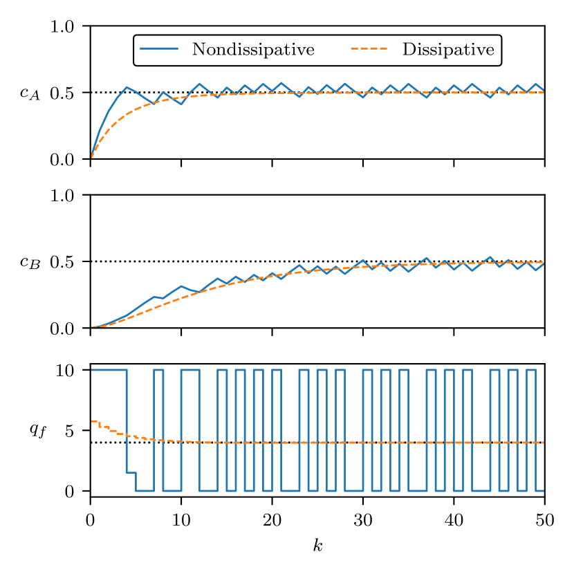
Figure 1: Nominal closed-loop trajectories for CSTR example with nondissipative and dissipative stage costs.

In Figure 2, we plot the closed-loop performance for 30 realizations of the disturbance trajectory. We define the closed-loop performance of these trajectories via the average economic stage cost:

$$\mathcal{J}_{T}=\frac{1}{T}\sum_{k=0}^{T-1}\ell(x(k),u(k))$$

in which $x(k)=\phi(k;x,\mathbf{w}_{\infty})$ and $u(k)=\kappa(x(k))$. Note that we evaluate the performance of both economic MPC formulations via only the economic (nondissipative) stage cost. For large $T$, we observe that the nondissipative stage cost produces better economic performance than the dissipative stage cost even when subject to perturbations.

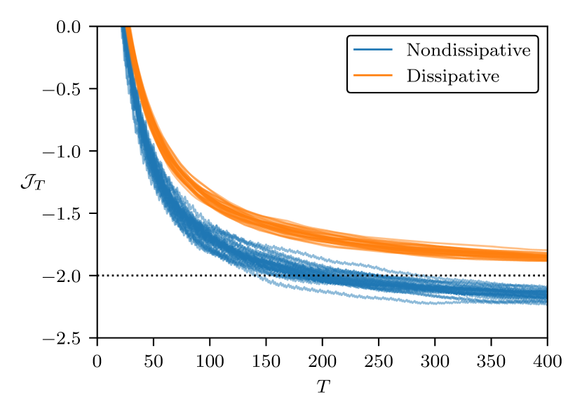
Figure 2: Closed-loop average economic performance for 30 realizations of disturbance trajectory with nondissipative and dissipative stage costs.

6 Future extensions

We plan to extend these results to suboptimal economic MPC algorithms that can be deployed online with limited computation time for high dimensional systems. Moreover, we can extend these results to time-varying systems and reference trajectories to address a wider class of problems. Many time-varying economic MPC applications do not require stability of a target reference trajectory and are instead primarily concerned with economic performance, e.g., HVAC or production scheduling.

References

• Alamir and Pannocchia (2021) Alamir, M. and Pannocchia, G. (2021). A new formulation of economic model predictive control without terminal constraint. Automatica, 125, 109420.
• Allan et al. (2017) Allan, D.A., Bates, C.N., Risbeck, M.J., and Rawlings, J.B. (2017). On the inherent robustness of optimal and suboptimal nonlinear MPC. Systems & Control Letters, 106, 68–78.
• Amrit et al. (2011) Amrit, R., Rawlings, J.B., and Angeli, D. (2011). Economic optimization using model predictive control with a terminal cost. Annual Reviews in Control, 35(2), 178–186.
• Angeli et al. (2011) Angeli, D., Amrit, R., and Rawlings, J.B. (2011). On average performance and stability of economic model predictive control. IEEE transactions on automatic control, 57(7), 1615–1626.
• Bayer et al. (2016) Bayer, F.A., Lorenzen, M., Müller, M.A., and Allgöwer, F. (2016). Robust economic model predictive control using stochastic information. Automatica, 74, 151–161.
• Berberich et al. (2020) Berberich, J., Köhler, J., Allgöwer, F., and Müller, M.A. (2020). Dissipativity properties in constrained optimal control: A computational approach. Automatica, 114, 108840.
• Diehl et al. (2010) Diehl, M., Amrit, R., and Rawlings, J.B. (2010). A lyapunov function for economic optimizing model predictive control. IEEE Transactions on Automatic Control, 56(3), 703–707.
• Dong and Angeli (2020) Dong, Z. and Angeli, D. (2020). Homothetic tube-based robust offset-free economic model predictive control. Automatica, 119, 109105.
• Faulwasser and Bonvin (2015) Faulwasser, T. and Bonvin, D. (2015). On the design of economic NMPC based on approximate turnpike properties. In 2015 54th IEEE Conference on Decision and Control (CDC), 4964–4970. IEEE.
• Grimm et al. (2004) Grimm, G., Messina, M.J., Tuna, S.E., and Teel, A.R. (2004). Examples when nonlinear model predictive control is nonrobust. Automatica, 40(10), 1729–1738.
• Grüne (2013) Grüne, L. (2013). Economic receding horizon control without terminal constraints. Automatica, 49(3), 725–734.
• Grüne and Müller (2016) Grüne, L. and Müller, M.A. (2016). On the relation between strict dissipativity and turnpike properties. Systems & Control Letters, 90, 45–53.
• Grüne and Pirkelmann (2020) Grüne, L. and Pirkelmann, S. (2020). Economic model predictive control for time-varying system: Performance and stability results. Optimal Control Applications and Methods, 41(1), 42–64.
• McAllister and Rawlings (2023) McAllister, R.D. and Rawlings, J.B. (2023). A suboptimal economic model predictive control algorithm for large and infrequent disturbances. IEEE Transactions on Automatic Control.
• Müller and Grüne (2016) Müller, M.A. and Grüne, L. (2016). Economic model predictive control without terminal constraints for optimal periodic behavior. Automatica, 70, 128–139.
• Pirkelmann et al. (2019) Pirkelmann, S., Angeli, D., and Grüne, L. (2019). Approximate computation of storage functions for discrete-time systems using sum-of-squares techniques. IFAC-PapersOnLine, 52(16), 508–513.
• Rawlings et al. (2020) Rawlings, J.B., Mayne, D.Q., and Diehl, M. (2020). Model predictive control: theory, computation, and design. Nob Hill Publishing Madison, WI.
• Schwenkel et al. (2020) Schwenkel, L., Köhler, J., Müller, M.A., and Allgöwer, F. (2020). Robust economic model predictive control without terminal conditions. IFAC-PapersOnLine, 53(2), 7097–7104.
• Yu et al. (2014) Yu, S., Reble, M., Chen, H., and Allgöwer, F. (2014). Inherent robustness properties of quasi-infinite horizon nonlinear model predictive control. Automatica, 50(9), 2269–2280.
• Zanon and Faulwasser (2018) Zanon, M. and Faulwasser, T. (2018). Economic MPC without terminal constraints: Gradient-correcting end penalties enforce asymptotic stability. Journal of Process Control, 63, 1–14.
• Zanon et al. (2016) Zanon, M., Gros, S., and Diehl, M. (2016). A tracking MPC formulation that is locally equivalent to economic MPC. Journal of Process Control, 45, 30–42.