On the impact of coordinated fleets size on traffic efficiency

Abstract

We investigate a traffic assignment problem on a transportation network, considering both the demands of individual drivers and of a large fleet controlled by a central operator (minimizing the fleet’s average travel time). We formulate this problem as a two-player convex game and we study how the size of the coordinated fleet, measured in terms of share of the total demand, influences the Price of Anarchy (PoA). We show that, for two-terminal networks, there are cases in which the fleet must reach a minimum share before actually affecting the PoA, which otherwise remains unchanged. Moreover, for parallel networks, we prove that the PoA is monotonically non-increasing in the fleet share.

I Introduction

Traffic assignment problems typically assume that traffic demand consists of drivers exhibiting selfish behavior to minimize travel time. However, technological advancements have introduced new services (ride-sourcing services, navigation apps) that, due to their widespread adoption, can influence the behavior of a substantial portion of drivers, potentially leading to a paradigm shift. Specifically, the providers of such services may leverage their position to minimize overall fleet metrics, such as total travel time, rather than optimizing individual user experiences. This approach, while potentially disadvantaging some users, aims to attract and retain users by providing lower travel times on average. In the following, we refer to groups of vehicles controlled by a central operator aiming to minimize the fleet’s average travel time as coordinated fleets. This work aims to study the impact that the presence of a coordinated fleet has on traffic efficiency in terms of the price of anarchy (PoA).

Contribution

We formulate the problem as a two-player game, with one player associated with the individual users and the other with the coordinated fleet. We study this game by using a well-known reformulation in terms of solution to a Variational Inequality (VI) (see [1, 2]). Specifically, we establish conditions ensuring that the operator of the VI associated to our game is strongly monotone. On the one hand, strong monotonicity ensures equilibrium uniqueness. On the other hand, through this property we are able to provide meaningful insights about the relationship between traffic efficiency and the share of the coordinated fleet in two-terminal networks. Using the Price of Anarchy (PoA) as a measure of traffic efficiency [3], we prove that the unique equilibrium and the PoA are Lipschitz continuous functions of the fleet share. Additionally, we derive sufficient conditions for the existence of a minimum share below which the presence of a coordinated fleet has no effect on traffic efficiency. Finally, for parallel networks, we show that the PoA, the flow of individual users, and the shortest travel time at equilibrium are monotonically non-increasing functions of the fleet share, suggesting improved efficiency for larger fleet share.

Related work

The multi-class traffic assignment problem was initially defined in [4]. Coordination among users of the same class was introduced in [5], where sufficient conditions for equilibrium existence and uniqueness are established, and then extended to more general settings in [6]. The impact on efficiency of coordinated classes was first considered in [7] for a three-class problem with:

• individual users, aiming at reducing individual travel time;

• a coordinated fleet, aiming at reducing overall fleet travel time; and

• a system-optimal fleet, aiming at reducing the system’s average travel time.

Numerical simulations in [7] show that sufficiently large coordinated and system-optimal fleets can lead to system optimality even in the presence of individual users.

Two-class problems are considered in [8, 9, 10, 11, 12]. Specifically, [8, 9, 10] consider a two-class problem, with individual users and a system-optimal fleet: [8] and [9] derived methods to compute the minimum share of system-optimal users necessary to induce system optimality, while [10] studied the trade-off between the magnitude of the improvement and the cost of deployment for the network manager.

More closely related to our contribution, [11] and [12] both consider a two-class problem with individual users and one coordinated fleet. In [11], sufficient conditions for equilibrium existence and uniqueness are derived. Such conditions are slightly weaker than the ones we use in this paper and are not sufficient to ensure strong monotonicity, which is instead crucial in our analysis. Their work also proposes two algorithms for the computation of the equilibrium and a control scheme to converge to the equilibrium in a dynamical framework.

Similarly to our work, in [12], the authors study the impact of coordinated fleets on traffic efficiency. First, they provide an example on a network with multiple origin-destination pairs and show that coordinated fleets can have detrimental effects on efficiency. Then, they investigate the minimum fleet size necessary to achieve system optimality and the maximum fleet size for which the user equilibrium persists, developing mathematical programs to compute them. They also provide analytical results about the threshold effect associated with the coordinated fleet size on efficiency, but only for parallel networks. In our work, instead, conditions under which a minimum size of the coordinated fleet is needed to affect the PoA are provided for general networks with a single origin-destination pair. Moreover, we derive results about the monotonicity of the PoA in the case of parallel networks.

Paper organization

The model and the main concepts are defined in Section II. Strong monotonicity, existence and uniqueness conditions are given in Section III. Section IV discusses the effect of a coordinated fleet on traffic efficiency as a function of the fleet size. Section V contains numerical studies illustrating our theoretical findings and providing interesting insights about extending this work to more general settings. Section VI contains concluding remarks and future perspectives.

II A two-class routing game

The transportation network is modeled as a directed graph $\mathcal{G}=(\mathcal{N},\mathcal{L})$, with node set $\mathcal{N}$ and link set $\mathcal{L}$, with links representing roads of the network and nodes representing junctions between them. Let $\mathcal{O}\subseteq\mathcal{N}$, called origins, be the subset of nodes from which exogenous traffic demands can access the network. Analogously, let $\mathcal{D}\subseteq\mathcal{N}$, called destinations, be the subset of nodes through which traffic can exit the network. Define the set of origin-destination pairs (OD pairs) $\mathcal{K}=\{(o,d)\,|\,o\in\mathcal{O},d\in\mathcal{D}\}$. Let $\mathcal{P}_{k}$ denote the set of paths associated with OD pair $k$ and let $\mathcal{P}:=\cup_{k\in\mathcal{K}}\mathcal{P}_{k}$. Let $N$, $L$, $K$, $P_{k}$ and $P$ be the cardinalities of $\mathcal{N}$, $\mathcal{L}$, $\mathcal{K}$, $\mathcal{P}_{k}$ and $\mathcal{P}$, respectively. Let $A$ be the link-path incidence matrix defined as

$$A_{lp}=\begin{cases}1,&l\in p\\ 0,&l\notin p\end{cases}.$$ (1)

Suppose now that $\mathcal{G}$ supports two classes of demand, namely class $S$ and class $C$. Class $S$ consists of selfish individual users, whereas class $C$ consists of a coordinated fleet. Let $D^{i}$ be the total demand of class $i,\ i=S,\,C$. Each OD pair $k$ is associated with a fraction $D^{i}_{k}>0,\ i=S,\,C$, of the total demand, i.e, $\sum_{k\in\mathcal{K}}D^{i}_{k}=D^{i}$. Let $D:=D^{S}+D^{C}$ be the total demand. For each class $i\in\{S,\,C\}$, we define the flow vector of class $i$ $z^{i}\in\mathbb{R}_{\geq 0}^{P}$ representing the traffic assignment of traffic demand $D^{i}$ over the network paths. The set of feasible flows of class $i$ is

$$\mathcal{Z}^{i}:=\biggl{\{}z^{i}\in\mathbb{R}_{\geq 0}^{P}\,:\,\sum_{p\in\mathcal{P}_{k}}z_{p}^{i}=D_{k}^{i},\ \forall k\in\mathcal{K}\biggl{\}}$$

and let $\mathcal{Z}=\mathcal{Z}^{S}\times\mathcal{Z}^{C}$. Each flow vector $z^{i}$ is associated with the load vector of class $i$ ($f^{i}:=Az^{i},\ i=S,\,C$) representing the load of each link of the network for class $i$. Then, the set of feasible loads of class $i$ is

$$\mathcal{F}^{i}:=\{f^{i}\in\mathbb{R}_{\geq 0}^{L}\,:\,f^{i}=Az^{i},\text{ for some }z^{i}\in\mathcal{Z}^{i}\}$$

and let $\mathcal{F}=\mathcal{F}^{S}\times\mathcal{F}^{C}$. Let the flow vector $z:=(z^{S},z^{C})$ and the load vector $f:=(f^{S},f^{C})$ be the concatenations of the flow and load vectors of the two classes and let $Z:=z^{S}+z^{C}$, $F:=f^{S}+f^{C}$ be the aggregate flow and load vectors, respectively. The assignment of the two classes of vehicles is determined by the delay functions characterizing the network links.

Definition 1 (Delay functions)

For every $l\in\mathcal{L}$, the delay $d_{l}:\mathbb{R}_{\geq 0}\rightarrow\mathbb{R}_{\geq 0}$ of link $l$ is a non-negative, strictly increasing and $C^{2}([0,+\infty))$ function with $d_{l}^{\prime}(0)>0$, depending on the aggregate flow $F_{l}$ on link $l$ only. Moreover, for every $p\in\mathcal{P}$, the function $d_{p}:\mathbb{R}^{L}_{\geq 0}\rightarrow\mathbb{R}_{\geq 0}$ is the delay of path $p$ and corresponds to the sum of the delays of the links included in $p$:

$$d_{p}(F)=\sum_{l\in\mathcal{L}}A_{lp}d_{l}(F_{l}).$$ (2)

The fact that link delays depend only on the aggregate load means that the two classes of vehicles affect the link delays in the same way.

We are interested in characterizing the equilibrium loads of the traffic assignment problem emerging from the interaction of the vehicle classes $S$ and $C$. To do this, we reformulate the problem as a two-player game, by associating each class to a strategic player. The strategy of each player corresponds to the load vector $f^{i}$ with strategy set $\mathcal{F}^{i},\ i=S,\,C$, respectively. The cost functions that player $S$ and player $C$ have to minimize in order to attain the goals of the traffic assignment problem are the following:

$$U^{S}(f):=\sum_{l\in\mathcal{L}}\,\int_{0}^{{f_{l}^{S}}}d_{l}(r+{f_{l}^{C}})dr,$$ (3)

$$U^{C}(f):=\sum_{l\in\mathcal{L}}\,f_{l}^{C}\cdot d_{l}(F_{l}).$$ (4)

In deriving the cost function for player $S$ we used a well-know reformulation of the Wardrop equilibrium of strategic agents in class $S$ as an optimization problem (with potential function as in (3)),[13, Chapter 3]. The cost of the player $C$ instead is the total travel time of vehicles in class $C$.

Definition 2 (Equilibria)

An equilibrium load of the two-class congestion game is a load vector $f^{*}=({f^{S}}^{*},{f^{C}}^{*})$ such that

$${f^{S}}^{*} :=\operatorname*{arg\,min}_{f^{S}\in\mathcal{F}^{S}}\ U^{S}(f^{S},{f^{C}}^{*}),\quad$$ (5)

$${f^{C}}^{*} :=\operatorname*{arg\,min}_{f^{C}\in\mathcal{F}^{S}}\ U^{C}({f^{S}}^{*},f^{C}).$$

All the feasible flows $z^{*}=({z^{S}}^{*},{z^{C}}^{*})$ such that $f^{*i}=Az^{*i},\ i=S,\,C$ are called equilibrium flow.

Note that from the fundamental theorem of calculus,

$$f_{l}^{C}\cdot d_{l}(F_{l})=\int_{0}^{f_{l}^{C}}(d_{l}({f_{l}^{S}}+r)+r\cdot d_{l}^{\prime}({f_{l}^{S}}+r))\,dr.$$

Hence (4) can be rewritten as

$$U^{C}(f)=\sum_{l\in\mathcal{L}}\,\int_{0}^{f_{l}^{C}}(d_{l}({f_{l}^{S}}+r)+r\cdot d_{l}^{\prime}({f_{l}^{S}}+r))\,dr.$$ (6)

The functions inside the integral in (6), that is,

$$m_{l}(f_{l}):=d_{l}(F_{l})+f_{l}^{C}\cdot d_{l}^{\prime}(F_{l}).$$ (7)

are known as marginal delay functions [3, Chapter 18].

We prove that under appropriate assumptions on the marginal delays $m_{l}(f_{l})$, the game in (5) is convex.

Lemma 1

$U^{S}(f)$ is convex in $f^{S}$ for any $f^{C}$. Moreover, if

$$\frac{\partial m_{l}(f_{l})}{\partial f_{l}^{C}}>0,\quad\forall f_{l}^{S},\,f_{l}^{C}\geq 0,\ \forall l\in\mathcal{L},$$ (8)

then $U^{C}(f)$ is convex in $f^{C}$ for any $f^{S}$.

Proof:

First, since $d_{l}$ is twice continuously differentiable, $\forall l\in\mathcal{L}$, the same is true for $U^{s}$. The Hessian matrix of $U^{S}$ with respect to $f^{S}$ is

$$\nabla^{2}U^{S}(f)=\mathrm{diag}\left(d_{l}^{\prime}(F_{l})\right)\succ 0$$

Hence, $U^{s}$ is convex in $f^{S}$, for any $f^{C}$. As for $U^{C}$, condition (8) ensures that its Hessian matrix with respect to $f^{C}$ is positive definite:

$$\nabla^{2}U^{C}(f)=\mathrm{diag}\left(\frac{\partial m_{l}(f_{l})}{\partial f_{l}^{C}}\right)\succ 0$$

Hence, $U^{C}$ is convex in $f^{C}$, for any $f^{S}$. ∎

Remark 1

The convexity of the cost functions (3) and (4) implies that any equilibrium flow $z^{*}$ must satisfy the following Wardrop conditions [13, Chapter 3]:

$${z^{S}_{p}}^{*}>0\Rightarrow\sum_{l\in\mathcal{L}}A_{lp}d_{l}(F_{l}^{*})\leq\sum_{l\in\mathcal{L}}A_{lr}d_{l}(F_{l}^{*}),\ \forall r\in\mathcal{P},$$ (9)

$${z^{C}_{p}}^{*}>0\Rightarrow\sum_{l\in\mathcal{L}}A_{lp}m_{l}(f_{l}^{*})\leq\sum_{l\in\mathcal{L}}A_{lr}m_{l}(f_{l}^{*}),\ \forall r\in\mathcal{P}.$$ (10)

In words, at equilibrium, each vehicle in class $S$ uses a path among those of shortest delay, whereas each vehicle in class $C$ uses a path among those of shortest marginal delay. Conditions (9) and (10) will be of key importance when proving the results in Section IV.

III Variational Inequality formulation and strong monotonicity

Under condition (8), the two-class routing game is convex and is equivalent to the following variational inequality (VI) [1, Proposition 1.4.2]:

$$(\phi-f^{*})^{\top}H(f^{*})\geq 0,\quad\forall\phi\in\mathcal{F},$$ (11)

where

$$H(f)=\left((d_{l}(F_{l}))_{l\in\mathcal{L}},(m_{l}(f_{l}))_{l\in\mathcal{L}}\right),$$ (12)

that is, equilibria of the two-class routing game correspond to solutions of (11).

The main result of this section consists in providing sufficient conditions for the operator $H$ of such VI to be strongly monotone on $\Omega:=[0,D]^{2L}\supset\mathcal{F}$, that is, for guaranteeing that

$$\exists c>0\,:\,(H(x)-H(y))^{\top}(x-y)\geq c||x-y||^{2},\ \forall x,y\in\Omega.$$ (13)

The strong monotonicity of $H$ not only ensures the uniqueness of the solution of (11) [1, Theorem 2.3.3], but also allows us to assess the impact of the fleet size onto traffic efficiency, as we shall demonstrate in the next section.

Proposition 1

The operator $H$ in (12) is strongly monotone on $\Omega$ if (8) holds and

$$d^{\prime}_{l}(F_{l})>\frac{1}{4}\frac{\partial m_{l}(f_{l})}{\partial f_{l}^{C}},\quad\forall f_{l}^{S},\,f_{l}^{C}\geq 0,\ \forall l\in\mathcal{L}.$$ (14)

Proof:

From [1, Proposition 2.3.2], we know that the operator $H$ is strongly monotone on an open set $\mathcal{U}$ if and only if its jacobian matrix is uniformly positive definite on $\mathcal{U}$, i.e.,

$$\exists\eta>0:\ \phi^{\top}J_{H}(f)\phi\geq\eta||\phi||^{2},\ \forall\phi\in\mathbb{R}_{+}^{2\cdot|\mathcal{L}|},\ \forall f\in\mathcal{U}.$$

The condition above is equivalent to

$$\exists\eta>0:\ J_{H}(f)-\eta I\succeq 0,\ \forall f\in\mathcal{U}.$$ (15)

Our proof proceeds in two steps: i) using the fact above we show that (14) implies that $H$ is strongly monotone on $\mathrm{int}(\Omega)$, ii) we show that strong monotonicity extends to $\Omega$ by continuity.

i) We study the positive semi-definiteness of $J_{H}-\eta I$ by examining its symmetric part $J_{H}^{\mathrm{sym}}(f)-\eta I$, where $J_{H}^{\mathrm{sym}}(f)$ is the symmetric part of $J_{H}$. Define

$$\Sigma_{1}(f):=\operatorname{diag}(d_{l}^{\prime}(F_{l}))-\eta I,$$

$$\Sigma_{2}(f):=\operatorname{diag}\left(\frac{1}{2}\frac{\partial m_{l}(f_{l})}{\partial f_{l}^{C}}\right),$$

$$\Sigma_{3}(f):=\operatorname{diag}\left(\frac{\partial m_{l}(f_{l})}{\partial f_{l}^{C}}\right)-\eta I,$$

then

$$J_{H}^{\operatorname{sym}}(f)-\eta I=\begin{pmatrix}\Sigma_{1}(f)&\Sigma_{2}(f)\\ \Sigma_{2}(f)&\Sigma_{3}(f)\end{pmatrix},$$

where we used the identity $d_{l}^{\prime}(F_{l})+\frac{\partial m_{l}(f_{l})}{\partial f_{l}^{S}}=\frac{\partial m_{l}(f_{l})}{\partial f_{l}^{C}}$. If $\Sigma_{1}(f)$ is positive definite, then $J_{H}^{\operatorname{sym}}(f)-\eta I$ is positive semi-definite if and only if its Schur complement $\Sigma(f):=\Sigma_{3}(f)-(\Sigma_{1}(f))^{-1}\Sigma_{2}^{2}(f)$ is. $\Sigma_{1}(f)$ and $\Sigma(f)$ are positive definite and positive semi-definite in $\mathrm{int}(\Omega)$, respectively, if the following conditions hold for all $l\in\mathcal{L}$:

$$d_{l}^{\prime}(F_{l})-\eta>0,\quad\forall f_{l}^{S},\,f_{l}^{C}\in(0,D),$$ (16)

$$\frac{\partial m_{l}(f_{l})}{\partial f_{l}^{C}}-\eta-\frac{\left(\frac{\partial m_{l}(f_{l})}{\partial f_{l}^{C}}\right)^{2}}{4(d_{l}^{\prime}(F_{l})-\eta)}\geq 0,\quad\forall f_{l}^{S},\,f_{l}^{C}\in(0,D).$$ (17)

By Definition 2,

$$\exists\eta_{1}>0\,:\,\eta_{1}<\min_{l\in\mathcal{L}}\min_{f_{l}^{S},\,f_{l}^{C}\in[0,D]}d_{l}^{\prime}(F_{l}).$$

Hence (16) holds for any $\eta\leq\eta_{1}$. Now, let

$$K_{l}(\eta,f_{l})=\frac{\partial m_{l}(f_{l})}{\partial f_{l}^{C}}-\eta-\frac{\left(\frac{\partial m_{l}(f_{l})}{\partial f_{l}^{C}}\right)^{2}}{4(d_{l}^{\prime}(F_{l})-\eta)},$$

$$K(\eta):=\min_{l\in\mathcal{L}}\min_{f_{l}^{S},\,f_{l}^{C}\in[0,D]}K_{l}(\eta,f_{l}).$$

We aim at proving that $K(\eta)>0$ for $\eta$ small enough, as that would imply (17). To this end, observe that given (8), (14) is equivalent to

$$\frac{\partial m_{l}(f_{l})}{\partial f_{l}^{C}}-\frac{\left(\frac{\partial m_{l}(f_{l})}{\partial f_{l}^{C}}\right)^{2}}{4d_{l}^{\prime}(F_{l})}>0,\quad\forall f_{l}^{S},\,f_{l}^{C}\geq 0,\ \forall l\in\mathcal{L}.$$

Since the l.h.s of the above condition is continuous in $f_{l}$ and the condition holds strictly for every $l\in\mathcal{L}$ and any $f_{l}^{S},\,f_{l}^{C}\in[0,D]$, then $K(0)>0$. We next prove that $K(\eta)$ is continuous in $\eta\in I=[0,\eta_{1})$ by showing that

$$K_{l}(\eta):=\min_{f_{l}^{S},\,f_{l}^{C}\in[0,D]}K_{l}(\eta,f_{l})$$

is continuous, for every $l$. By continuity in both arguments of $K_{l}(\eta,f_{l})$, for every $\epsilon>0$,

$$\exists\delta>0\,:\,|\eta-\mu|+||f_{l}-g_{l}||<\delta\Rightarrow|K_{l}(\eta,f_{l})-K_{l}(\mu,g_{l})|<\epsilon.$$ (18)

Take $\eta_{3},\,\eta_{4}\in I$ such that $|\eta_{3}-\eta_{4}|<\delta$ and define the minimizers $f_{l}^{\eta_{i}}\in[0,D]^{2}:K_{l}(\eta_{i},f_{l}^{\eta_{i}})=K_{l}(\eta_{i})$. Then, by (18) with $f_{l}=g_{l}=f_{l}^{\eta_{i}}$ we obtain

$$0\leq|K_{l}(\eta_{i},f_{l}^{\eta_{i}})-K_{l}(\eta_{j},f_{l}^{\eta_{i}})|<\epsilon,\ \ i=3,4,\ i\neq j.$$

Hence,

$$K_{l}(\eta_{i},f_{l}^{\eta_{i}})>K_{l}(\eta_{j},f_{l}^{\eta_{i}})-\epsilon\geq K_{l}(\eta_{j})-\epsilon,\ i=3,4,\ i\neq j.$$

The above implies

$$K_{l}(\eta_{i})>K_{l}(\eta_{j})-\epsilon,\quad i=3,4,\ i\neq j.$$

Combining the two conditions above we get

$$|K_{l}(\eta_{3})-K_{l}(\eta_{4})|<\epsilon.$$

Hence, $K_{l}(\eta)$ is continuous, $\forall l\in\mathcal{L}$, thus $K(\eta)$ is continuous, as it is point-wise minimum of continuous functions.

The continuity of $K(\eta)$ together with $K(0)>0$, implies that there exists $\eta_{2}$ such that (17) is satisfied for all $l\in\mathcal{L}$, for any $\eta\in[0,\eta_{2})$. The existence of $\eta_{1}$ and $\eta_{2}$ ensure the existence of $\eta>0$ such that (16) and (17) hold for all $l\in\mathcal{L}$. Therefore, there exists a $\eta$ small enough such that (15) holds on $\mathrm{int}(\Omega)$, thus $H$ is strongly monotone in $\mathrm{int}(\Omega)$:

$$\exists c>0\,:\,(H(\tilde{x})-H(\tilde{y}))^{\top}(\tilde{x}-\tilde{y})\geq c||\tilde{x}-\tilde{y}||^{2},\ \forall\tilde{x},\tilde{y}\in\mathrm{int}(\Omega).$$ (19)

ii) Now, observe that $\mathrm{cl}(\mathrm{int}(\Omega))=\Omega$. Then, consider any $x,y\in\Omega$ and let $\{x^{(n)}\},\,\{y^{(n)}\}\subset\mathrm{int}(\Omega)$ be two sequences converging to $x$ and $y$, respectively. Then,

$$(H(x^{(n)})-H(y^{(n)}))^{\top}(x^{(n)}-y^{(n)})\geq c||x^{(n)}-y^{(n)}||^{2},\ \forall n.$$

By taking the limit and using the continuity of $H$,

$$(H(x)-H(y))^{\top}(x-y)\geq c||x-y||^{2}.$$

This means that strong monotonicity of $H$ extends to $\Omega$. ∎

The strong monotonicity of $H$ ensures the uniqueness of the solution of (11), that is, of the equilibrium load $f^{*}$. In [11], weaker conditions similar to (14) were derived to ensure the uniqueness of the equilibrium load. Our slightly stronger conditions are needed to guarantee that $H$ is strongly monotone and that thus the following assumption holds.

Assumption 1

Suppose that the operator $H$ in (12) is Lipschitz and strongly monotone in $\Omega=[0,D]^{2L}$.

Again, we remark that sufficient conditions for strong monotonicity to hold are given in Proposition 14, whereas Lipschitz continuity follows from the smoothness of delay and marginal delay functions (defined on a compact set).

Remark 2

A class of delay functions that satisfy conditions (8) and (14), thereby ensuring strong monotonicity of (12), consists of polynomial functions of degree at most $3$ with non-negative coefficients and strictly positive derivatives on $[0,+\infty)$, see [11] for similar examples. This demonstrates that assuming strong monotonicity is not too restrictive, as this property holds for a relevant class of delay functions.

IV Price of Anarchy

The total delay experienced by all the vehicles travelling across the network is defined as

$$T(f):=\sum_{l\in\mathcal{L}}F_{l}\cdot d_{l}(F_{l}).$$ (20)

A feasible load minimizing $T(f)$ is called an optimal load (denoted by $F^{\omega}\in\mathcal{F}$). Then, the Price of Anarchy is defined as the ratio between the total delay attained at the (unique under Assumption 1) equilibrium $f^{*}$ and the minimum total delay:

$$\operatorname*{PoA}:=\frac{\sum_{l\in\mathcal{L}}F_{l}^{*}\cdot d_{l}(F_{l}^{*})}{\sum_{l\in\mathcal{L}}F_{l}^{\omega}\cdot d_{l}(F_{l}^{\omega})}\geq 1.$$ (21)

We aim to study how the size of the coordinated fleet affects the $\mathrm{PoA}$. From now on, we focus our attention on two-terminal networks.

Assumption 2

The network has a single OD pair. Let $D^{S}=(1-\alpha)D$ and $D^{C}=\alpha D$ represent the demand of class $S$ and $C$ entering the network from its unique origin, where $\alpha$ is the share of class $C$, which we refer to as the fleet share.

We provide three main results in this section. First, we prove that the equilibrium load and the PoA are Lipschitz continuous functions of the fleet share $\alpha$. Second, we derive a sufficient condition for the existence of a minimum fleet share below which the coordinated fleet has no impact on the PoA. Finally, we show that the PoA of the equilibrium load is a non-increasing function of $\alpha$ for the case of parallel networks. To make explicit their dependence on $\alpha$, we will indicate the feasible set by $\mathcal{F}(\alpha)$ the equilibrium load as $f^{*}(\alpha)$ and we will indicate as $\mathrm{PoA}(\alpha),\ d_{l}(\alpha),\ m_{l}(\alpha)$ the PoA and the associated delay and marginal delay functions at equilibrium.

IV-A Lipschitz continuity

Proposition 2

Let Assumptions 1 and 2 hold. The equilibrium load $f^{*}(\alpha)$ is Lipschitz continuous in $\alpha$, i.e., there exists $k>0$ such that

$$\forall\alpha_{1},\alpha_{2},\quad||f^{*}(\alpha_{2})-f^{*}(\alpha_{1})||\leq k|\alpha_{2}-\alpha_{1}|.$$ (22)

Proof:

Assume w.l.o.g. that $\alpha_{1}<\alpha_{2}$. Define $v:=(-v^{S},v^{C})$, where

$$v^{S}:=\frac{\alpha_{2}-\alpha_{1}}{1-\alpha_{1}}{f^{S}}^{*}(\alpha_{1}),\quad v^{C}:=\frac{\alpha_{2}-\alpha_{1}}{\alpha_{2}}{f^{C}}^{*}(\alpha_{2}),$$

are scaled versions of ${f^{S}}^{*}(\alpha_{1})$ and ${f^{C}}^{*}(\alpha_{2})$, respectively, both associated with a total demand equal to $(\alpha_{2}-\alpha_{1})D$ and such that

$$0\leq v^{S}\leq{f^{S}}^{*}(\alpha_{1}),\quad 0\leq v^{C}\leq{f^{C}}^{*}(\alpha_{2}).$$

Since $v^{S}$ and $v^{C}$ are both associated with a total demand equal to $(\alpha_{2}-\alpha_{1})D$, it must hold that

$$0\leq v^{i}_{l}\leq(\alpha_{2}-\alpha_{1})D,\quad\forall l\in\mathcal{L},\ i=S,\,C,$$

which implies that $||v||^{2}\leq 2LD^{2}(\alpha_{2}-\alpha_{1})^{2}.$ Hence $||v||\leq k^{\prime}|\alpha_{2}-\alpha_{1}|$, with $k^{\prime}=\sqrt{2L}D$. Now, define

$$f^{(1)}=f^{*}(\alpha_{2})-v\in\mathcal{F}(\alpha_{1}),\quad f^{(2)}=f^{*}(\alpha_{1})+v\in\mathcal{F}(\alpha_{2}).$$

By (11), one can write

$$(f^{(i)}-f^{*}(\alpha_{i}))^{\top}H(f^{*}(\alpha_{i}))\geq 0,\quad i=1,2.$$

By summing these two inequalities and using the definition of $f^{(i)}$, one gets

$$(H(f^{*}(\alpha_{2}))-H(f^{*}(\alpha_{1})))^{\top}v\geq$$ (23)

$$(H(f^{*}(\alpha_{2}))-H(f^{*}(\alpha_{1})))^{\top}(f^{*}(\alpha_{2})-f^{*}(\alpha_{1}))\geq$$

$$c||f^{*}(\alpha_{2})-f^{*}(\alpha_{1})||^{2},$$

where the last line follows from strong monotonicity of $H$ over $\Omega$ (notice that $\mathcal{F}(\alpha_{i})\subset\Omega,\ i=1,2$). From Cauchy-Schwartz inequality and (23)

$$c||f^{*}(\alpha_{2})-f^{*}(\alpha_{1})||^{2}\leq||H(f^{*}(\alpha_{1}))-H(f^{*}(\alpha_{2}))||\,||v||\leq$$

$$\leq Q\cdot||f^{*}(\alpha_{1})-f^{*}(\alpha_{2})||\cdot k^{\prime}|\alpha_{2}-\alpha_{1}|,$$

where $Q$ is the Lipschitz constant of $H$. The proof is complete by picking $k=Qk^{\prime}/c$. ∎

Since the PoA is Lipschitz continuous in the equilibrium load and the flows are defined on a bounded set, the PoA is also a Lipschitz continuous function of $\alpha$.

IV-B Critical fleet share

A first question that one may ask is if introducing a coordinated fleet always helps in reducing the PoA. In this section, we show that this is not the case. Specifically, we derive a sufficient condition under which there is a positive minimum critical fleet size needed to induce changes in the PoA.

Theorem 1 (Critical fleet size)

Let $\mathcal{P}^{i}(z(\alpha))$ indicate the set of paths used by class $i$ at the equilibrium flow $z(\alpha)$, $i=C,S$, respectively. Let Assumptions 1 and 2 hold. Suppose that $\exists\tilde{\alpha}\in(0,1)$ such that $f^{*}(\tilde{\alpha})$ admits an equilibrium flow $z^{*}(\tilde{\alpha})$ such that $\mathcal{P}^{C}(z^{*}(\tilde{\alpha}))\subseteq\mathcal{P}^{S}(z^{*}(\tilde{\alpha}))$. Then,

$$f^{*}(\alpha)=\left({f^{S}}^{*}(\tilde{\alpha})+\frac{\tilde{\alpha}-\alpha}{\tilde{\alpha}}{f^{C}}^{*}(\tilde{\alpha}),\frac{\alpha}{\tilde{\alpha}}{f^{C}}^{*}(\tilde{\alpha})\right),$$ (24)

and $\mathrm{PoA}(\alpha)=\mathrm{PoA}(0),\ \forall\alpha\in[0,\tilde{\alpha}]$.

Proof:

Consider the equilibrium load $f^{*}(\tilde{\alpha})$ and the associated equilibrium flow $z^{*}(\tilde{\alpha})$. Clearly,

$${z_{p}^{S}}^{*}(\tilde{\alpha})>0\Rightarrow\sum_{l\in\mathcal{L}}A_{lp}d_{l}(\tilde{\alpha}) \leq\sum_{l\in\mathcal{L}}A_{l\gamma}d_{l}(\tilde{\alpha}),\ \forall\gamma\in\mathcal{P},$$ (25)

$${z_{p}^{C}}^{*}(\tilde{\alpha})>0\Rightarrow\sum_{l\in\mathcal{L}}A_{lp}m_{l}(\tilde{\alpha}) \leq\sum_{l\in\mathcal{L}}A_{l\gamma}m_{l}(\tilde{\alpha}),\ \forall\gamma\in\mathcal{P}.$$

Consider the following feasible flow (obtained by moving part of the flow from C to S):

$$z^{*}(\alpha)=\left({z^{S}}^{*}(\tilde{\alpha})+\frac{\tilde{\alpha}-\alpha}{\tilde{\alpha}}{z^{C}}^{*}(\tilde{\alpha}),\,\frac{\alpha}{\tilde{\alpha}}{z^{C}}^{*}(\tilde{\alpha})\right).$$ (26)

We show that $z^{*}(\alpha)$ is an equilibrium flow when the fleet share is $\alpha$, i.e.,

$${z_{p}^{S}}^{*}(\alpha)>0\Rightarrow\sum_{l\in\mathcal{L}}A_{lp}d_{l}(\alpha) \leq\sum_{l\in\mathcal{L}}A_{l\gamma}d_{l}(\alpha),\ \forall\gamma\in\mathcal{P},$$ (27)

$${z_{p}^{C}}^{*}(\alpha)>0\Rightarrow\sum_{l\in\mathcal{L}}A_{lp}m_{l}(\alpha) \leq\sum_{l\in\mathcal{L}}A_{l\gamma}m_{l}(\alpha),\ \forall\gamma\in\mathcal{P}.$$

We prove each of the above conditions. The first easily follows after noticing that i) $z^{*}(\alpha)$ and $z^{*}(\tilde{\alpha})$ induce the same aggregate load, i.e., $F_{l}^{*}(\alpha)=F_{l}^{*}(\tilde{\alpha})$, so none of the path delays has changed, and ii) the set of paths used by vehicles in class $S$ is the same, i.e., $\mathcal{P}^{S}(z^{*}(\tilde{\alpha}))=\mathcal{P}^{S}(z^{*}(\alpha))$ (since $\mathcal{P}^{C}(z^{*}(\tilde{\alpha}))\subseteq\mathcal{P}^{S}(z^{*}(\tilde{\alpha}))$ ). Hence, the first inequality in (25) ensures that all vehicles in class $S$ still use shortest delay paths. As for the second condition, similarly, one has to prove that vehicles in class $C$ still use shortest marginal delay paths. Because of the expression of (26), one can observe that:

• $\mathcal{P}^{C}(z^{*}(\alpha))=\mathcal{P}^{C}(z^{*}(\tilde{\alpha}))\subseteq\mathcal{P}^{S}(z^{*}(\tilde{\alpha}))$;

• for every $p\in\mathcal{P}$, since the aggregate loads have not changed, the marginal delay is

  $$m_{p}(\alpha)=\sum_{l\in\mathcal{L}}A_{lp}\left(d_{l}(\tilde{\alpha})+\frac{\alpha}{\tilde{\alpha}}{f_{l}^{C}}^{*}(\tilde{\alpha})d_{l}^{\prime}(\tilde{\alpha})\right),$$

By multiplying the first inequality in (25) by $1-\alpha/\tilde{\alpha}$, the second one by $\alpha/\tilde{\alpha}$, then summing them, one obtains

$$m_{p}(\alpha) =\sum_{l\in\mathcal{L}}A_{lp}\left(d_{l}(\tilde{\alpha})+\frac{\alpha}{\tilde{\alpha}}{f_{l}^{C}}^{*}(\tilde{\alpha})d_{l}^{\prime}(\tilde{\alpha})\right)\leq$$ (28)

$$\leq\sum_{l\in\mathcal{L}}A_{l\gamma}\left(d_{l}(\tilde{\alpha})+\frac{\alpha}{\tilde{\alpha}}{f_{l}^{C}}^{*}(\tilde{\alpha})d_{l}^{\prime}(\tilde{\alpha})\right)=m_{\gamma}(\alpha),$$

$\forall p\in\mathcal{P}^{C}(z^{*}(\alpha)),\ \forall\gamma\in\mathcal{P}$. Hence, every $\mathcal{P}^{C}(z^{*}(\alpha))$ is still a shortest marginal delay path. Therefore, $z^{*}(\alpha)$ is a equilibrium flow when the fleet share is equal to $\alpha$. The equilibrium load associated with $z^{*}(\alpha)$ is

$$f^{*}(\alpha)=\left({f^{S}}^{*}(\tilde{\alpha})+\frac{\tilde{\alpha}-\alpha}{\tilde{\alpha}}{f^{C}}^{*}(\tilde{\alpha}),\frac{\alpha}{\tilde{\alpha}}{f^{C}}^{*}(\tilde{\alpha})\right),$$

which must correspond to the unique equilibrium of the problem.

To conclude, notice that for all $\alpha\in[0,\tilde{\alpha}]$ all links have the same aggregate load. Hence $\mathrm{PoA}(\alpha)=\mathrm{PoA}(0)$ for all $\alpha\in[0,\tilde{\alpha}]$. ∎

IV-C PoA monotonicity for Parallel Networks

In this section, we show that the PoA is non-increasing in the fleet share $\alpha$ under the following assumptions.

Assumption 3

$\mathcal{G}$ is a parallel network, that is, it consists of an OD pair connected by finitely many links directed from the origin node to the destination node. Again let $\alpha$ be the fleet share.

Assumption 4

The delay function $d_{l}$ is convex, $\forall l\in\mathcal{L}$.

The assumption of parallel networks simplifies the analysis as, in that case, the notion of link and path coincides. The convexity of the delay functions instead ensures that $d^{\prime}_{l}(F_{l})$ is non-decreasing in $F_{l}$. Note that in particular this implies the following monotonicity property

$$\bar{F}_{l}>F_{l}\ \textup{and}\ \bar{f}^{C}_{l}>f^{C}_{l}\quad\Rightarrow\quad m_{l}(\bar{f}_{l})>m_{l}(f_{l}).$$ (29)

Let $\theta(\alpha)$ and $\mu(\alpha)$ indicate the minimum delay and the minimum marginal delay realised at equilibrium when the fleet share is $\alpha$, respectively. Observe that, since links and paths coincide, the equilibrium condition implies

$$l\in\mathcal{L}^{S}(\alpha)\Rightarrow d_{l}(F_{l}^{*}(\alpha))=\theta(\alpha),$$

$$l\in\mathcal{L}^{C}(\alpha)\Rightarrow m_{l}(f_{l}^{*}(\alpha))=\mu(\alpha).$$

Proposition 3

Let Assumptions 1, 3 and 4 hold. Suppose there exists $\alpha_{1},\alpha_{2}\in(0,1)$ such that $\alpha_{1}<\alpha_{2}$ and $\mathcal{L}^{S}(\alpha_{1})=\mathcal{L}^{S}(\alpha_{2})$ and $\mathcal{L}^{C}(\alpha_{1})=\mathcal{L}^{C}(\alpha_{2})$. Then,

1. $\theta(\alpha_{1})\geq\theta(\alpha_{2})$;

2. $\mu(\alpha_{1})\leq\mu(\alpha_{2})$;

3. ${f_{l}^{S}}^{*}(\alpha_{1})\geq{f_{l}^{S}}^{*}(\alpha_{2}),\ \forall l\in\mathcal{L}$;

4. ${f_{l}^{C}}^{*}(\alpha_{1})\leq{f_{l}^{C}}^{*}(\alpha_{2}),\ \forall l\in\mathcal{L}$.

Proof:

Since $\mathcal{L}^{i}(\alpha_{1})=\mathcal{L}^{i}(\alpha_{2}),\ i=S,\,C$, let us indicate both as $\mathcal{L}^{i},\ i=S,\,C$ for convenience. Along with them, consider also the set $\mathcal{L}^{C\setminus S}:=\mathcal{L}^{C}\setminus(\mathcal{L}^{S}\cap\mathcal{L}^{C})$, corresponding to the set of links used by class $C$ only. Notice that also this set remains constant in passing from $\alpha_{1}$ to $\alpha_{2}$. Also, since it is used by vehicles of class $C$ only,

$${f_{l}^{C}}^{*}(\alpha_{i})=F_{l}^{*}(\alpha_{i}),\ \forall l\in\mathcal{L}^{C\setminus S},\ i=1,2.$$ (30)

We distinguish two cases: If $\mathcal{L}^{C\setminus S}=\emptyset$ the conclusion follows from Theorem 1. We next discuss the case in which $\mathcal{L}^{C\setminus S}\neq\emptyset$.
1) By contradiction, suppose that $\theta(\alpha_{1})<\theta(\alpha_{2})$. This implies that the aggregate load increased on all links in $\mathcal{L}^{S}$, i.e., $F_{l}^{*}(\alpha_{1})<F_{l}^{*}(\alpha_{2}),\ \forall l\in\mathcal{L}^{S}$. Now, since the demand of class $S$ decreased, there must exist a link $j\in\mathcal{L}^{S}$ such that the load of class $S$ on it decreased, i.e., ${f_{j}^{S}}^{*}(\alpha_{1})>{f_{j}^{S}}^{*}(\alpha_{2})$. The latter fact, combined with the increase of the aggregate loads on all link in $\mathcal{L}^{S}$, implies that the load of class $C$ on link $j$ increased, i.e., ${f_{j}^{C}}^{*}(\alpha_{1})<{f_{j}^{C}}^{*}(\alpha_{2})$. By (29), the increase of both the aggregate load and the load of class $C$ on link $j$ implies that its marginal delay increased. Hence, $\mu(\alpha_{1})<\mu(\alpha_{2})$.

On the other hand, the fact that the aggregate load increased on all links in $\mathcal{L}^{S}$ implies that the aggregate demand directed toward the set $\mathcal{L}^{S}$ increased, which is equivalent to say that the aggregate demand toward the set $\mathcal{L}^{C\setminus S}$ decreased. Then, there must be at least one link $e\in\mathcal{L}^{C\setminus S}$ whose aggregate load decreased, i.e., $F_{e}^{*}(\alpha_{1})>F_{e}^{*}(\alpha_{2})$. From (30), this is equivalent to ${f_{e}^{C}}^{*}(\alpha_{1})>{f_{e}^{C}}^{*}(\alpha_{2})$, which implies that $\mu(\alpha_{1})>\mu(\alpha_{2})$, contradicting what proved above. Therefore, $\theta(\alpha_{1})\geq\theta(\alpha_{2})$.
2) From 1), $\theta(\alpha_{1})\geq\theta(\alpha_{2})$, which implies that the aggregate load on none of the links in $\mathcal{L}^{S}$ can increase. This implies that the aggregate demand toward $\mathcal{L}^{S}$ cannot increase, which is equivalent to say that the aggregate demand toward $\mathcal{L}^{C\setminus S}$ cannot decrease. From (30), this means that the demand associated with class $C$ directed toward $\mathcal{L}^{C\setminus S}$ did not decreased. Hence, there exists $e\in\mathcal{L}^{C\setminus S}$ such that ${f_{e}^{C}}^{*}(\alpha_{1})\leq{f_{e}^{C}}^{*}(\alpha_{2})$. Hence, $\mu(\alpha_{1})\leq\mu(\alpha_{2})$.

3) By contradiction, suppose that $\exists l\in\mathcal{L}^{S}\ |\ {f^{S}_{l}}^{*}(\alpha_{1})<{f^{S}_{l}}^{*}(\alpha_{2})$. Since on all links in $\mathcal{L}^{S}$ the aggregate load did not increase ($F_{l}(\alpha_{1})\geq F_{l}(\alpha_{2})$), the above implies that ${f^{C}_{l}}^{*}(\alpha_{1})>{f^{C}_{l}}^{*}(\alpha_{2})$. This implies $\mu(\alpha_{1})>\mu(\alpha_{2})$, contradicting point 2).
4) Suppose that there $\exists l\in\mathcal{L}^{C}\,|\,{f_{l}^{C*}(\alpha_{1})}>{f_{l}^{C*}(\alpha_{2})}$. By point 3) we also know that ${f_{l}^{S*}(\alpha_{1})}\geq{f_{l}^{S*}(\alpha_{2})}$. Hence ${F_{l}(\alpha_{1})}>{F_{l}(\alpha_{2})}$. By (29), this implies $\mu(\alpha_{1})>\mu(\alpha_{2})$, which contradicts 2). ∎

Remark 3

The result above and its proof implicitly assumes that $(\mathcal{L}^{S}\cap\mathcal{L}^{C})\neq\emptyset$. To see that this is always true, assume by contradiction that $(\mathcal{L}^{S}\cap\mathcal{L}^{C})=\emptyset$. Then, it follows

$$\forall l\in\mathcal{L}^{S}(\alpha),\quad m_{l}(f_{l}^{*}(\alpha))=d_{l}(F_{l}^{*}(\alpha))=\theta(\alpha),$$

$$\forall e\in\mathcal{L}^{C}(\alpha),\quad m_{e}(f_{e}^{*}(\alpha))>d_{e}(F_{e}^{*}(\alpha))\geq\theta(\alpha),$$

which is impossible as vehicles in class $C$ at equilibrium must use links of minimal marginal delay.

Proposition 4

Let Assumptions 1, 3 and 4 hold. Suppose there exists $\alpha_{1},\alpha_{2}\in(0,1)$ such that $\alpha_{1}<\alpha_{2}$ and $\mathcal{L}^{S}(\alpha_{1})=\mathcal{L}^{S}(\alpha_{2})$ and $\mathcal{L}^{C}(\alpha_{1})=\mathcal{L}^{C}(\alpha_{2})$. Then, $\mathrm{PoA}(\alpha_{1})\geq\mathrm{PoA}(\alpha_{2})$.

Proof:

First of all, notice that it suffices to consider only the numerator (20) of $\mathrm{PoA}$, as its denominator is constant. The numerator (20) can be written as follows:

$$T(f^{*}(\alpha)) =\sum_{l\in\mathcal{L}}{f^{S}_{l}}^{*}(\alpha)\cdot d_{l}(\alpha)+\sum_{l\in\mathcal{L}}{f^{C}_{l}}^{*}(\alpha)\cdot d_{l}(\alpha)=:$$

$$:=T^{S}(f^{*}(\alpha))+T^{C}(f^{*}(\alpha)).$$

From 1) of Proposition 3,

$$T^{S}(f^{*}(\alpha_{2})) =\sum_{l\in\mathcal{L}}{f^{S}_{l}}^{*}(\alpha_{2})\cdot d_{l}(F^{*}_{l}(\alpha_{2}))=$$ (31)

$$=\theta(\alpha_{2})\sum_{l\in\mathcal{L}}{f^{S}_{l}}^{*}(\alpha_{2})\leq$$

$$\leq\theta(\alpha_{1})\sum_{l\in\mathcal{L}}{f^{S}_{l}}^{*}(\alpha_{2})=$$

$$=\sum_{l\in\mathcal{L}}{f^{S}_{l}}^{*}(\alpha_{2})\cdot d_{l}(F_{l}^{*}(\alpha_{1})).$$

Moreover, because of 3) of Proposition 3, one can observe that

$${f^{C}}^{*}(\alpha_{1})+({f^{S}}^{*}(\alpha_{1})-{f^{S}}^{*}(\alpha_{2}))\in\mathcal{F}^{C}(\alpha_{2}).$$

Therefore, if one defines $\varphi:={f^{S}}^{*}(\alpha_{1})-{f^{S}}^{*}(\alpha_{2})\geq 0$:

$$T^{C}(f^{*}(\alpha_{2})) =\sum_{l\in\mathcal{L}}{f^{C}_{l}}^{*}(\alpha_{2})\cdot d_{l}(F^{*}_{l}(\alpha_{2}))\leq$$ (32)

$$\leq\sum_{l\in\mathcal{L}}({f_{l}^{C}}^{*}(\alpha_{1})+\varphi)\cdot d_{l}(F_{l}^{*}(\alpha_{1})),$$

where the inequality follows from the fact ${f^{C}_{l}}^{*}(\alpha_{2})$ minimizes $\sum_{l\in\mathcal{L}}f^{C}_{l}\cdot d_{l}({f^{S}_{l}}^{*}(\alpha_{2})+f^{C}_{l})$. The proof is concluded after noticing that summing the inequalities (31) and (32) one gets

$$T(f^{*}(\alpha_{2})) \leq\sum_{l\in\mathcal{L}}({f_{l}^{S}}^{*}(\alpha_{1})+{f_{l}^{C}}^{*}(\alpha_{1}))\cdot d_{l}(F_{l}^{*}(\alpha_{1}))=$$

$$=\sum_{l\in\mathcal{L}}F_{l}^{*}(\alpha_{1})\cdot d_{l}(F_{l}^{*}(\alpha_{1}))=T(f^{*}(\alpha_{1})).$$

∎

Theorem 2 (PoA monotonicity)

Let Assumptions 1, 3 and 4 hold. $\mathrm{PoA}(\alpha)$ is non-increasing in the fleet share $\alpha$.

Proof:

Proposition 22 establishes that the equilibrium load $f^{*}(\alpha)$ is a Lipschitz continuous function of $\alpha$ and Proposition 4 ensures that on any interval over which the support of the two vehicles classes is constant, the flow of links used by class $S$ can only decrease and that of class $C$ can only increase. Hence it must be that for any $\alpha_{1}<\alpha_{2}$, $\mathcal{L}^{S}(\alpha_{2})\subseteq\mathcal{L}^{S}(\alpha_{1})$ and $\mathcal{L}^{C}(\alpha_{1})\subseteq\mathcal{L}^{C}(\alpha_{2})$. Since there are a finite number of links, there are a finite number of points in which the support of either class S or C changes. Since: i) the $\mathrm{PoA}$ is Lipschitz continuous, ii) it is non-increasing with $\alpha$ for any interval in which the support doesn’t change and iii) the support changes in a finite number of points, one can conclude that the $\mathrm{PoA}$ is non-increasing with $\alpha$ everywhere. ∎

V Examples

Below, we present two examples. The first example aims to illustrate the theoretical results presented in the preceding section. The second example, on the other hand, aims to suggest which results can be expected to persist in more general contexts and which may not.

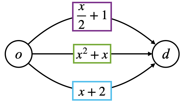
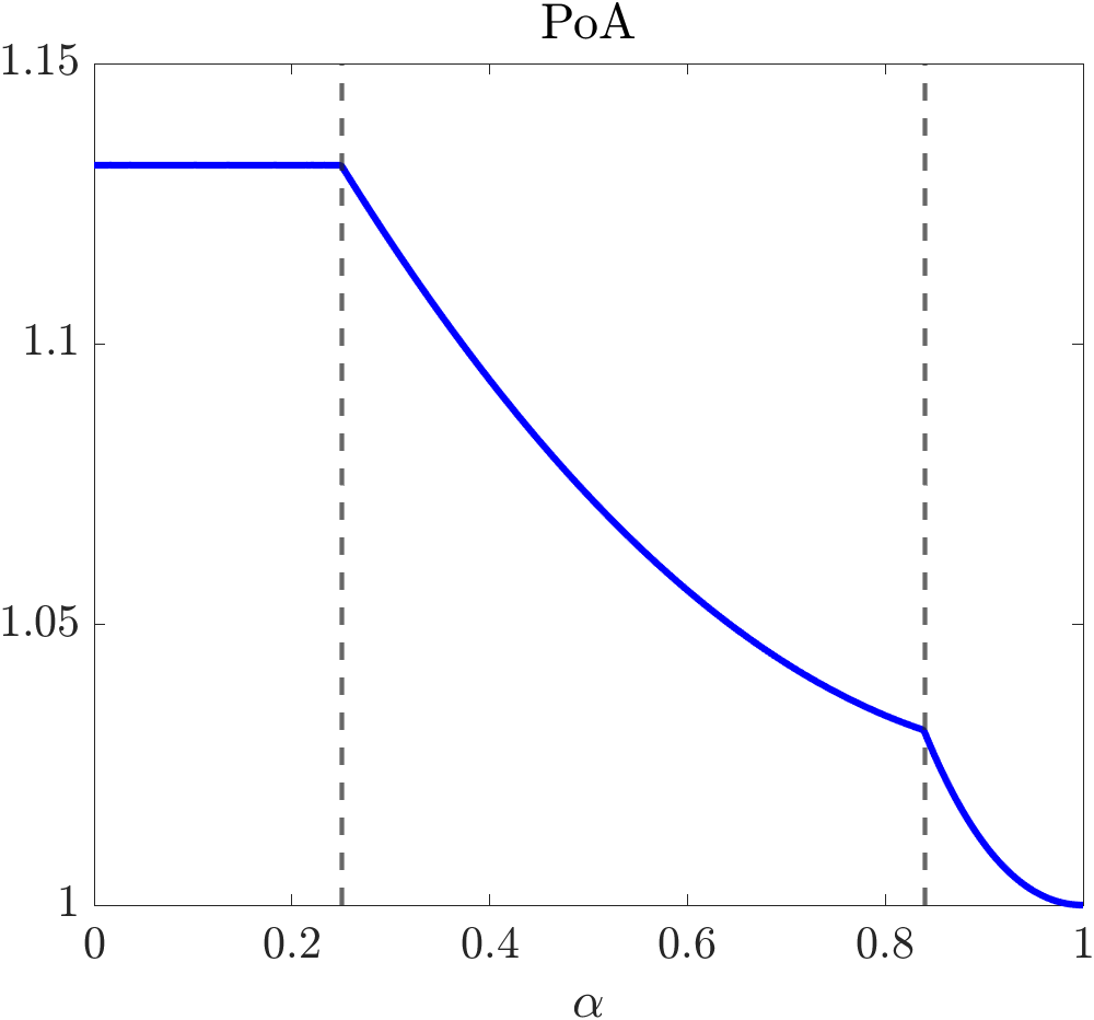
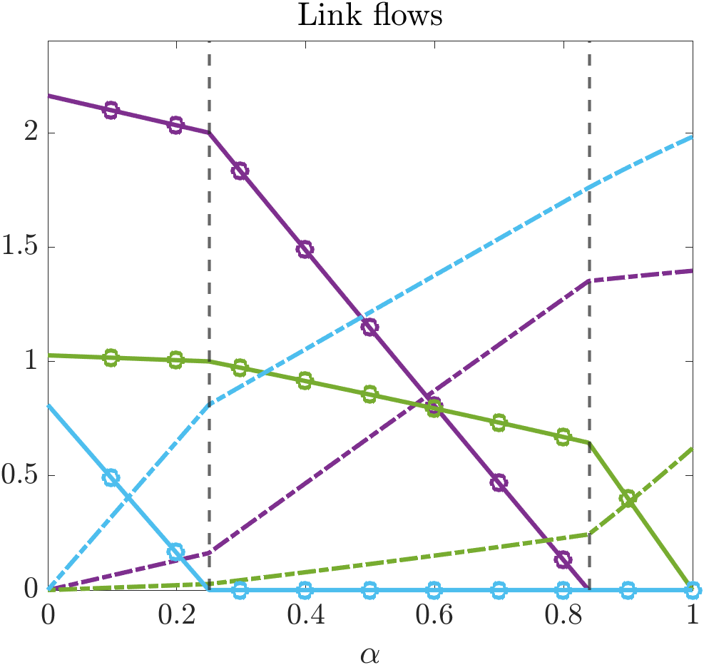
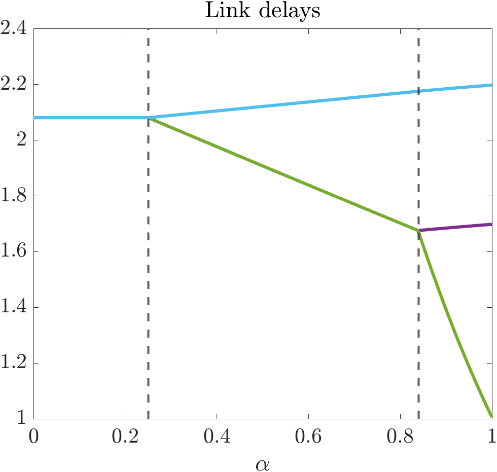
Figure 1: Example of parallel network. Link labels stand for the link delays. We set $D=4$. In the bottom row, violet lines refer to the top link, green lines refer to the middle link and light-blue lines refer to the bottom link. Solid lines with circles refer to the flows associated with class $S$, while dashed lines to those associated with class $C$. Finally, the vertical gray dashed lines identify the changes occurring in the support of the two vehicle classes as $\alpha$ varies.

Example 1

Consider the example in Figure 1. The plots showcase the evolution of the $\mathrm{PoA}(\alpha)$, the equilibrium loads ${f_{l}^{i}}^{*}(\alpha),\ l=1,2,3,\ i=S,\,C$, and the link delays $d_{l}(\alpha),\ l=1,2,3$, as functions of $\alpha$, for $\alpha$ varying in $[0,1]$. According to Proposition 3 and Theorem 2, the three plots demonstrate that Price of Anarchy, the flows associated with class $S$ and the minimum delay at equilibrium are non-increasing in the fleet share $\alpha$, while the flows associated with class $C$ are non-decreasing in $\alpha$. Notice also that, as long as $\alpha\leq\tilde{\alpha}\approx 0.25$, the support of $C$ is included in that of $S$ and $\mathrm{PoA}(\alpha)=\mathrm{PoA}(0)$ for any $\alpha\leq\tilde{\alpha}$, consistently with Theorem 1. Hence this is an example in which a minimum fleet size ($\tilde{\alpha}$) is needed for affecting the PoA.

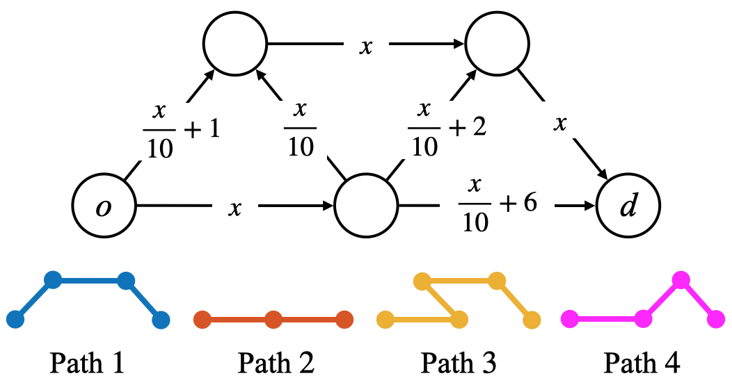
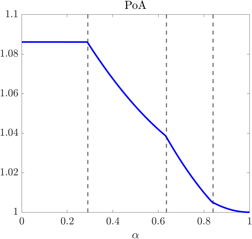
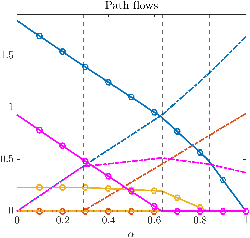
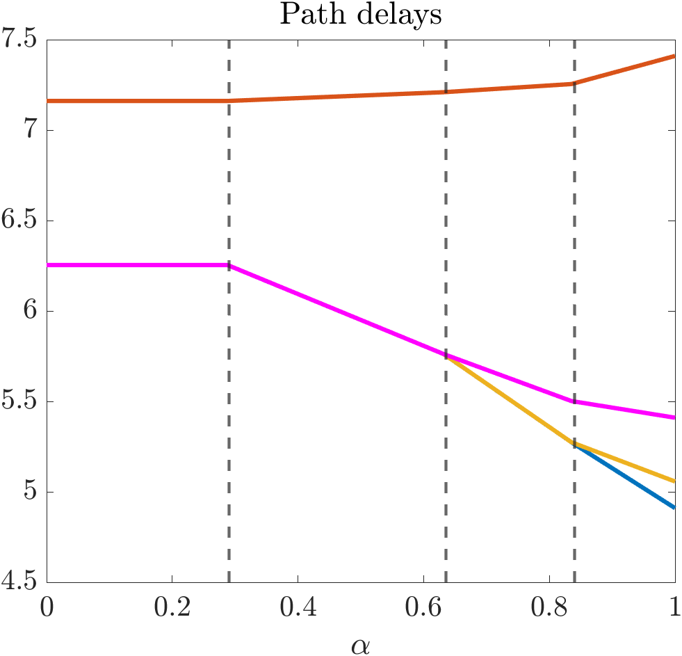
Figure 2: Example of network consisting of seven links and four paths. Link labels stand for the link delays. We set $D=3$. In the bottom row, blue lines refer to Path $1$, orange lines refer to Path $2$, yellow lines refer to Path $3$ and magenta lines to Path $4$. Solid circled lines refer to the flows associated with class $S$, while dashed lines to those associated with class $C$. Finally, the vertical grey dashed lines identify the changes occurring in the support of the two vehicle classes as $\alpha$ varies.

Example 2

Consider the example in Figure 2. The plots depict the behavior of the $\mathrm{PoA}(\alpha)$, the unique equilibrium path flows ${z_{p}^{i}}^{*}(\alpha),\ p=1,2,3,4,\ i=S,\,C$ and the path delays $d_{p}(\alpha),\ p=1,\dots,4$, as functions of $\alpha$, for $\alpha$ varying in $[0,1]$. Although not guaranteed in general, in this case uniqueness of the equilibrium flow $z^{*}(\alpha)$ follows from the uniqueness of the equilibrium load $f^{*}(\alpha),\ \forall\alpha\in[0,\,1]$. This is due to the fact that each path of the network in Figure 2 possesses a link not shared with any other path. This means that the load of a class on that link determines the flow of the class on the corresponding path. Hence, since the equilibrium load is unique, so is the equilibrium flow. Now, as in the parallel network case, the $\mathrm{PoA}$, the equilibrium flows associated with class $S$ and the minimum path delay are non-increasing with respect to $\alpha$. Different from parallel networks, we note that in this simulation the path flows associated with class $C$ are instead not necessarily monotone (see the flow of path 4). Whether monotonicity of the PoA can be proven in this more general case remains an open problem.

VI Conclusion

This study contributes to a better understanding of the impact exerted by coordinated fleets of vehicles on the efficiency of transportation networks. Under the assumption of strong monotonicity, for the case of two-terminal networks we highlight two phenomena. Firstly, we identify settings in which the coordinated fleet needs to reach a certain threshold of share in the total demand before affecting the PoA of the unique equilibrium load. Secondly, we proved that for parallel networks, the PoA weakly decreases as the share of the coordinated fleet increases.

The future perspectives we aim to explore are multiple. On the one hand, we would like to characterize more precisely the threshold phenomenon associated with coordinated fleet share, providing conditions that clearly outline the occurrence of this phenomenon. On the other hand, we would like to investigate whether the monotonicity of the PoA and equilibrium flows persists in the case of more general two-terminal networks, as suggested by the last example in Section V. Lastly, we also aspire to expand the discussion to networks with multiple origins and destinations. For this setting, we remark that [12] already proved that PoA monotonicity does not hold in general. Yet, we believe that establishing sufficient network conditions guaranteeing that the presence of coordinated fleets improves network efficiency would represent an important future contribution.

References

- [1] F. Facchinei and J.-s. Pang, Finite-dimensional variational inequalities and complementarity problems. New York, NY: Springer New York, 2003.
- [2] G. Scutari, D. P. Palomar, F. Facchinei, and J.-s. Pang, “Convex optimization, game theory, and variational inequality theory,” IEEE Signal Processing Magazine, vol. 27, no. 3, pp. 35–49, 2010.
- [3] N. Nisan, T. Roughgarden, E. Tardos, and V. V. Vazirani, Algorithmic Game Theory. New York, NY, USA: Cambridge University Press, 2007.
- [4] S. C. Dafermos, “The traffic assignment problem for multiclass-user transportation networks,” Transportation Science, vol. 6, no. 1, pp. 73–87, 1972.
- [5] P. T. Harker, “Multiple equilibrium behaviors on networks,” Transportation Science, vol. 22, no. 1, pp. 39–46, 1988.
- [6] T. Boulogne, E. Altman, H. Kameda, and O. Pourtallier, “Mixed equilibrium (ME) for multiclass routing games,” IEEE Transactions on Automatic Control, vol. 47, no. 6, pp. 903–916, 2002.
- [7] H. Yang, X. Zhang, and Q. Meng, “Stackelberg games and multiple equilibrium behaviors on networks,” Transportation Research Part B: Methodological, vol. 41, no. 8, pp. 841–861, 2007.
- [8] G. Sharon, M. Albert, T. Rambha, S. Boyles, and P. Stone, “Traffic optimization for a mixture of self-interested and compliant agents,” Proceedings of the AAAI Conference on Artificial Intelligence, vol. 32, no. 1, 2018.
- [9] Z. Chen, X. Lin, Y. Yin, and M. Li, “Path controlling of automated vehicles for system optimum on transportation networks with heterogeneous traffic stream,” Transportation Research Part C: Emerging Technologies, vol. 110, pp. 312–329, 2020.
- [10] K. Zhang and Y. M. Nie, “Mitigating the impact of selfish routing: An optimal-ratio control scheme (ORCS) inspired by autonomous driving,” Transportation Research Part C: Emerging Technologies, vol. 87, pp. 75–90, 2018.
- [11] G. Nilsson, P. Grover, and U. Kalabić, “Assignment and control of two-tiered vehicle traffic,” in 2018 IEEE Conference on Decision and Control (CDC), 2018, pp. 1023–1028.
- [12] M. Battifarano and S. Qian, “The impact of optimized fleets in transportation networks,” Transportation Science, vol. 57, no. 4, pp. 1047–1068, 2023.
- [13] A. Ozdaglar and I. Menache, Network games: Theory, Models and Dynamics. Williston, VT: Morgan & Claypool, 2011.