Speakable and unspeakable in quantum measurements

Abstract

ABSTRACT

Quantum mechanics, in its orthodox version, imposes severe limits on what can be known, or even said, about the condition of a quantum system between two observations. A relatively new approach, based on so-called “weak measurements”, suggests that such forbidden knowledge can be gained by studying the system’s response to an inaccurate weakly perturbing measuring device. It goes further to propose revising the whole concept of physics variables, and offers various examples of counterintuitive quantum behaviour. Both views go to the very heart of quantum theory, and yet are rarely compared directly. A new technique must either transcend the orthodox limits, or just prove that these limits are indeed necessary. We study both possibilities, and find for the orthodoxy.

But when you have no apparatus to determine through which hole the thing goes, then you cannot say that it either goes through one hole or the other. You can always say it - provided you stop thinking immediately and make no deductions from it. Physicists prefer not to say it, rather than stop thinking at the moment.

R.P. Feynman in Character of Physical Law

…we can separate, for example, the spin from the charge of an electron, or internal energy of an atom from the atom itself.

Y. Aharonov, S. Popescu, D. Rohrlich, and P. Skrzypczyk in Quantum Cheshire Cats

I Introduction

In 1963 FeynL ,1964 FeynC , and 1965 FeynH Feynman and co-authors outlined what they considered the most general principles of the quantum method. At about the same time, the authors of ABL proposed what is known as the “Aharonov, Bergmann, and Lebowitz rule” for calculating the probabilities of a pre- and post-selected quantum system. Feynman’s arguments are rarely revisited in a discussion of the quantum measurement theory. On the other hand, a recent development of the views expressed in ABL has given the reader the concept of “weak measurements”, and a plethora of “quantum paradoxes” the concept helps to establish (see, for example, SPIN100 -CAT2 ).
The attitude to asking questions about the quantum method is often summed by Mermin’s taunt “Shut up and calculate” MERM . Calculations are, no doubt, useful, but understanding the method’s limitations, could tell one something about the relation between a human observer and nature.
The purpose of this paper is to compare directly the orthodoxy of FeynL (one can hardly be more orthodox than when appealing to a reputable undergraduate text) with recent developments in the quantum measurement theory SPIN100 -CAT2 , REVIEW1 -MES4 . Our aim is to see whether anything new has indeed been added to the views expressed in FeynL - FeynH , or if at least some of these views have been disproved by the more recent research (a preliminary attempt of such a comparison was made in DSmyst ). It is easy to see DSABL that the original ABL rule is a particular example of the Feynman’s rule for assigning probabilities FeynL . A further comparison is more involved. Feynman’s reasoning is subtle, as one has to walk a “logical tightrope” in order to “interpret nature” FeynC . The centrepiece of the orthodox description is the Uncertainty Principle, best known in its Heisenberg form FeynL . According to the Principle, certain questions, easily answered in a classical context, should have no answer when dealing with a quantum system. In particular, very little may be said about the path taken by an unobserved particle in a double-slit experiment, FeynL , FeynC and, by the same token, about the state of any system between two observations. The authors of COMPL suggested that a meaningful description of a system between the measurements can be obtained by employing weakly perturbing detectors. (We refer the reader to Ref.Lund for a possible use of such detectors in order to surpass the Heisenberg limit in joint measurements of a particle’s position and momentum.) Over the years, the approach proposed in COMPL has lead to a number of spectacular claims COMPL -CAT2 , which we will submit to further scrutiny here.
The rest of the paper is organised as follows. In Sect. II we discuss consecutive quantum measurements, the need to produce records of the past outcomes, and a simplified description, possible if particular types of probes are used. Sect. III reviews the “orthodox” description of quantum behaviour, given in FeynL , FeynC , FeynH . In Sect. IV we use the description to analyse a quantum measurement analogy of the double-slit problem. In Sect. V we leave the narrative of FeynL , FeynC , FeynH , and discuss the “weak values”, first introduced in SPIN100 , as well as their possible interpretations. In Sect. VI we introduce a three-slit (“three-box”) system, and create our own “paradox”, similar to that proposed in 3BOX . In Sect. VII the “paradox” is dismissed for reasons explained in Sect. V. In Sect. VIII we revisit a four-slit (quantum Cheshire cat CAT1 , CAT2 ) problem. Sect. IX contains our conclusions. Appendices A and B contain the necessary technical details. To condense the presentation, we will bring in the proverbial Alice (an orthodox theorist), Bob (an experimenter), and Carol, a kind of “devil’s advocate”, who disagrees with Alice and asks her awkward questions. We apologise to the reader who may find these characters annoying.

II Bob wants to measure three quantities

Bob has a quantum system, and wants to measure, at times $t_{0}<t_{1}<t_{2}$, the quantities ${\bf A}$, ${\bf B}$, and ${\bf C}$, each taking certain number of discrete values $M_{A,B,C}\leq N$. He asks Alice the theorist to tell him how to do it, and what he is likely to see.
Alice tells him that at the end of the experiment, at $t=t_{2}$, he would need three visible records of the measured values (the system itself cannot provide this information). He would then measure the frequency with which a particular series of records occurs after many trials.
Alice’s mathematical task is to predict the said frequencies, and to do so she associates with the system an $N$-dimensional Hilbert space $\mathcal{H}^{S}$, and represents Bob’s quantities by Hermitian operators, $\hat{A}$, ${\hat{B}}$, and $\hat{C}$, acting therein. (If a classical calculation were to be made, she would consider a phase space, and dynamical functions of positions and momenta). There are three orthonormal eigenbases of $\hat{A}$, ${\hat{B}}$, and $\hat{C}$, $\left\{|a_{k}{\rangle}\right\}$, $\left\{|b_{l}{\rangle}\right\}$, and $\left\{|c_{n}{\rangle}\right\}$. The first measured quantity, she tells Bob, must not have degenerate eigenvalues, so that if the first measurement yields $A_{k}$, Alice knows that the system is “in a state $|a_{k}{\rangle}$”, and can proceed with her calculation. The second operator may have $M_{B}<N$ degenerate eigenvalues,

$$\hat{B}=\sum_{m=1}^{M_{B}}B_{m}\;\hat{\pi}(B_{m}),\quad\quad\hat{\pi}(B_{m})=\sum_{l=1}^{N}\Delta(B_{m}-{\langle}b_{l}|\hat{B}|b_{l}{\rangle})|b_{l}{\rangle}{\langle}b_{l}|,$$ (1)

where $\Delta(X-Y)=1$ if $X=Y$, and $0$ otherwise. The same applies to the third operator, $\hat{C}$, but for now we will assume that all $C_{n}$ are different.
Bob’s records are to be produced and kept by three probes $D^{A}$, ${D^{B}}$, and ${D^{C}}$, each with its own Hilbert space, $\mathcal{H}^{D^{A}}$, $\mathcal{H}^{D^{B}}$, and $\mathcal{H}^{D^{C}}$, so the large Hilbert space which Alice will use for her calculations is a tensor product of the four, $\mathcal{H}^{S+P}=\mathcal{H}^{S}\otimes\mathcal{H}^{D^{B}}\otimes\mathcal{H}^{D^{B}}\otimes\mathcal{H}^{D^{C}}$.
Alice also needs to construct a Hamiltonian $\hat{H}^{S+P}(t)$, and a unitary evolution operator, $\hat{U}^{S+P}=\exp[-i\int_{t_{0}}^{t_{2}}\hat{H}^{S+P}(t^{\prime})dt^{\prime}]$ (we use $\hbar=1$) , also acting in $\mathcal{H}^{S+P}$. The first probe, $D^{A}$, should briefly couple to the system at $t=t_{0}$, in such a manner that any initial product state $|D^{A}(0){\rangle}\otimes|\psi^{S}{\rangle}$ becomes

$$|D^{A}(0){\rangle}\otimes|\psi^{S}{\rangle}\to\sum_{k=1}^{N}{\langle}a_{k}|\psi^{S}{\rangle}|D^{A}(A_{k}){\rangle}\otimes|a_{k}{\rangle},\quad\quad\left({\langle}D^{A}(A_{k^{\prime}})|D^{A}(A_{k}){\rangle}=\delta_{k^{\prime}k}\right),$$ (2)

where $|D^{A}(0){\rangle}$ is the probe’s initial state, and its final condition $|D^{A}(A_{k}){\rangle}$ tells Bob that the outcome of the first measurement was $A_{k}$. The action of the second probe at $t=t_{1}$ is defined similarly,

$$|D^{B}(0){\rangle}\otimes|\psi^{S}{\rangle}\to\sum_{m=1}^{M_{B}}|D^{B}(B_{m}){\rangle}\otimes\hat{\pi}(B_{m})|\psi^{S}{\rangle},$$ (3)

whereas the third probe acts at $t=t_{2}$ according to (2). If the system has a non-zero time independent Hamiltonian, $\hat{H}^{S}$, between $t_{0}$ and $t_{1}$, and $t_{1}$ and $t_{2}$ it undergoes its own unitary evolution with an operator $\hat{U}^{S}(t,t^{\prime})=\exp[-i\hat{H}^{S}(t-t^{\prime})]$ (see Fig.1a).
It should be mentioned that at the beginning Bob has no prior knowledge of the system’s state $|\psi^{S}{\rangle}$ in Eq.(2). So for him the experiment begins when the first probe reads $A_{k}$. The necessary statistics can then be collected, e.g., by repeating the measurements on the same system, retaining only the cases where the first outcome is $A_{k}$. For Alice the initial state of the composite is $|D^{C}(0){\rangle}|D^{B}(0){\rangle}|D^{A}(A_{k}){\rangle}|a_{k}{\rangle}$, and the probability of having the entire sequence $\{C_{n}\leftarrow B_{m}\leftarrow A_{k}\}$ is given by (see Fig.1a, the $\otimes$s henceforth omitted)

$$P(C_{n}\leftarrow B_{m}\leftarrow A_{k})=$$

$$\sum_{j=1}^{N}\left|{\langle}D^{C}(C_{n})|{\langle}D^{B}(B_{m})|{\langle}D^{A}(A_{k})|{\langle}\phi^{S}_{j}|\hat{U}^{S+P}(t_{2},t_{0})|D^{C}(0){\rangle}|D^{B}(0){\rangle}|D^{A}(A_{k}){\rangle}|a_{k}{\rangle}\right|^{2},$$ (4)

so that $\sum_{n=1}^{N}\sum_{m=1}^{M_{B}}P(C_{n}\leftarrow B_{m}\leftarrow A_{k})=1$. The states $|\phi^{S}_{j}{\rangle}$ form an arbitrary orthonormal basis, and the choice $|\phi^{S}_{j}{\rangle}=|c_{j}{\rangle}$ simplifies the evaluation due to the appearance of a Kronecker $\delta_{jn}$ (see Fig.1b).
One can say that the operator $\hat{U}^{S+P}(t_{2},t_{0})$ describes an unbroken unitary evolution of the composite $\{system+probes\}$ from just after $t_{0}$ to just after $t_{2}$. Or one can simply say that Alice needs to know matrix elements of a unitary operator $\hat{U}^{S+P}(t_{2},t_{0})$ between particular states in the Hilbert space of the composite, and not mention the evolution at all DSreal .

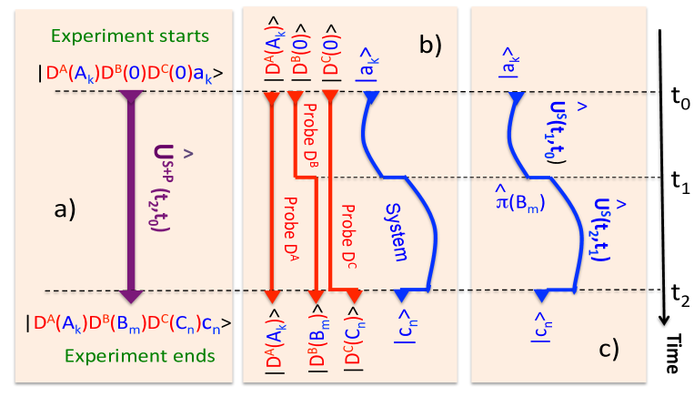
Figure 1: a) Unbroken unitary evolution of a composite $\{system+probes\}$ from $t_{0}$ to $t_{2}$ [cf. Eq.(II)]; b) a more detailed view of the evolution: the probes are coupled at $t_{0}$, $t_{1}$, and $t_{2}$, and carry the records until the experiment is finished; c) broken unitary evolution of the system only [cf. Eq.(6)].

Furthermore, the probabilities in Eq.(II) can be obtained without mentioning the probes explicitly, since the couplings (2) and (3) are simple, and their actions are easily taken into account (details can be found, e.g., in DSreal ). In particular, one has for the probability of measuring the sequence ($B_{m}$, $C_{n}$), provided the first detection gave $A_{k}$, an equally valid form,

$$P(C_{n}\leftarrow B_{m}\leftarrow A_{k})=|{\langle}c_{n}|\hat{U}^{S}(t_{2},t_{1})\hat{\pi}(B_{m})\hat{U}^{S}(t_{1},t_{0})|a_{k}{\rangle}|^{2},$$ (5)

if the measured eigenvalue of $\hat{C}$ is not degenerate. If it is, $\hat{C}=\sum_{\mu=1}^{M_{C}}C_{\mu}\hat{\pi}(C_{\mu})$, an additional summation is needed,

$$P(C_{\mu}\leftarrow B_{m}\leftarrow A_{k})=\sum_{n=1}^{N}\Delta(C_{\mu}-{\langle}c_{n}|\hat{C}|c_{n}{\rangle})|{\langle}c_{n}|\hat{U}^{S}(t_{2},t_{1})\hat{\pi}(B_{m})\hat{U}^{S}(t_{2},t_{1})|a_{k}{\rangle}|^{2}.$$ (6)

Thus, Alice has a choice. She may either consider an unbroken (except at $t=t_{2}$) unitary evolution of the composite $\{system+probes\}$ in a larger Hilbert space $\mathcal{H}^{S+P}$ [cf. Eq.(II)], or she may deal with an evolution in a smaller space $\mathcal{H}^{S}$, interrupted at $t=t_{1}$ by insertion of the projector $\hat{\pi}(B_{m})$ [cf. Eq.(6)]. This interruption is necessary to account for the action of Bob’s probe $D^{B}$ at $t=t_{1}$, and is by no means mysterious. This second option is clearly more practical.

III A different view of the same problem: the orthodoxy

Alice can also reconsider her problem in the light of the general principles of the quantum theory as laid out in FeynL , FeynC . These principles, we recall, are:

• The probability of an event is given by an absolute square of a complex valued probability amplitude. The amplitudes of two consecutive steps need to be multiplied.

• If the event can occur in different ways, and it is not possible to determine which of the alternatives is taken, the amplitudes for each way ought to be summed, and an interference pattern will emerge.

• If it is possible to determine, even in principle, whether one or the other alternative is taken, then the probabilities ought to be summed.

• The probabilities describe the state of the affairs when the experiment is “finished”.

• One never sums the amplitudes for different final states FOOT1 .

• Uncertainty Principle: one cannot determine which of the alternatives has been taken without destroying the interference pattern. FOOT2 .

In Alice’s case the event in question consists of preparing the system in a state $|a_{k}{\rangle}$ at $t=t_{0}$, and then finding it in a state $|c_{n}{\rangle}$ at $t=t_{2}$. At time $t_{1}$, $t_{0}<t_{1}<t_{2}$, the system can be deemed to be in one of the states $|b_{l}{\rangle}$, so there are, in principle, $N$ different ways (paths), $\{c_{n}\leftarrow b_{l}\leftarrow a_{k}\}$, $l=1,...,N$, in which the event may occur. Notice that $c_{n}$, $b_{l}$ and $a_{k}$ refer to states (lower case) and not to eigenvalues (upper case). By (a) the corresponding amplitudes are

$${\mathcal{A}}(c_{n}\leftarrow b_{l}\leftarrow a_{k})={\langle}c_{n}|\hat{U}^{S}(t_{2},t_{1})|b_{l}{\rangle}{\langle}b_{l}|\hat{U}^{S}(t_{1},t_{0})|a_{k}{\rangle},$$ (7)

and if no attempt is made to determine the state at $t=t_{1}$ the amplitudes should be added [cf. (b)], which yields ${\mathcal{A}}(c_{n}\leftarrow a_{k})=\sum_{l=1}^{N}{\mathcal{A}}(c_{n}\leftarrow b_{l}\leftarrow a_{k})={\langle}c_{n}|\hat{U}^{S}(t_{2},t_{1})|a_{k}{\rangle}$.
If at $t=t_{1}$ Bob measures a ${\hat{B}}$ with degenerate eigenvalues, the amplitudes of the paths passing through the eigenstates of ${\hat{B}}$ corresponding to the same $B_{m}$ cannot be distinguished, and, by (b) and (c), Eq.(5) follows. If some of the eigenvalues of $\hat{C}$ are also degenerate, the rule (e) prescribes adding the probabilities Eq.(5) for all the eigenstates $|c_{n}{\rangle}$ with the same eigenvalue $C_{\mu}$, which yields Eq.(6).
According to FeynL , the essence (the “only mystery”) of quantum mechanics is contained in the double-slit example. There a particle can reach a point on the screen via two holes, where the observed number of arrivals exhibits an interference pattern consisting of “bright” and “dark” fringes. Next we revisit the case in a slightly different context, and discuss it in some detail.

IV The double-slit case. The unspeakable and the barely speakable

To create a kind of a double-slit case in the context of quantum measurements, one needs three successive observations, similar to those discussed in Sect. II. [Measuring just two operators, $\hat{A}$ and ${\hat{B}}$, won’t do since, according to principle (e) in the previous section, there are no interesting interference effects.]
Allowing ${\hat{B}}$ to have only two different values, $B_{1}$ and $B_{2}$, and treating these alternatives as “slits”, creates two virtual paths connecting the “source” $|a_{k}{\rangle}$ with $N$ “points on the screen”, represented by $|c_{n}{\rangle}$. The corresponding amplitudes are ($m=1,2$)

$${\mathcal{A}}(c_{n}\leftarrow B_{m}\leftarrow a_{k})=\sum_{l=1}^{N}\Delta(B_{m}-{\langle}b_{l}|{\hat{B}}|b_{l}{\rangle}){\mathcal{A}}(c_{n}\leftarrow b_{l}\leftarrow a_{k}).$$ (8)

The “intensities” $W_{n}\equiv|{\mathcal{A}}(c_{n}\leftarrow B_{m}\leftarrow a_{k})|^{2}$, corresponding to being in state $|a_{k}{\rangle}$, measuring the value $B_{m}$, and finally being in state $|c_{n}{\rangle}$, may or may not show an “interference pattern”, depending on whether it is possible to determine which of the two alternatives occurred. The simplest case is, of course, a two-level system, $N=2$, with only two “final locations”, $|c_{1}{\rangle}$ and $|c_{2}{\rangle}$ (${\langle}c_{2}|c_{1}{\rangle}=0$) [see Fig 2a]. For an initial state $|a_{1}{\rangle}$, special choice $|c_{1}{\rangle}=\hat{U}^{S}(t_{2},t_{0})|a_{1}{\rangle}$, makes $|c_{1}{\rangle}$ and $|c_{2}{\rangle}$, the bright and dark fringes, respectively, since

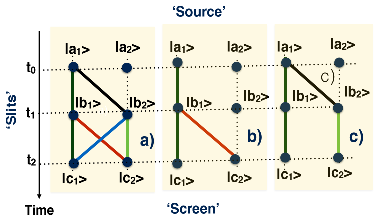
Figure 2: a) The simplest double-slit problem. Intermediate, of $|b_{1,2}{\rangle}$, and final, $|c_{1,2}{\rangle}$, play the role of the “slits”, and “points on the screen”, respectively. b) a special choice $|b_{1}{\rangle}=\hat{U}^{S}(t_{1},t_{0})|a_{1}{\rangle}$ eliminates two of the four virtual paths in a), and no interference is left in the system. c) similarly, choosing $|b_{1,2}{\rangle}=[\hat{U}^{S}(t_{2},t_{1})]^{-1}|c_{1,2}{\rangle}$ also reduces the number of paths to two.

$$W_{1}(\text{interference})=|{\mathcal{A}}(c_{1}\leftarrow b_{1}\leftarrow a_{1})+{\mathcal{A}}(c_{1}\leftarrow b_{2}\leftarrow a_{1})|^{2}={\langle}c_{1}|\hat{U}^{S}(t_{2},t_{1})|a_{1}{\rangle}=1,$$ (9)

$$W_{2}(\text{interference})=|{\mathcal{A}}(c_{2}\leftarrow b_{1}\leftarrow a_{1})+{\mathcal{A}}(c_{2}\leftarrow b_{2}\leftarrow a_{1})|^{2}={\langle}c_{2}|\hat{U}^{S}(t_{2},t_{1})|a_{1}{\rangle}=0.$$

IV.1 Closing one slit

In FeynL Feynman pointed out the need for a “special language”, required to describe the double-slit conundrum. Firstly, the slit chosen by the particle cannot be pre-determined by a “hidden” variable. Were it so, closing one of the slits could only decrease the number of particles arriving at a given point (see also Bohr1 ). This, however, would be a wrong prediction since the closure makes the particles arrive at a previously dark spot. Consequently, it is not possible to say that the particle goes through one slit, and not the other. The same happens in our simple example. Although we cannot literally block one of the slits, it is possible to redirect the system, passing via $|b_{1}{\rangle}$ or $|b_{2}{\rangle}$ to different destinations, e.g., by measuring ${\hat{B}}$, and counting separately the cases where the result is $B_{1}$ or $B_{2}$. By (c) of Sect. III, knowing the value of ${\hat{B}}$ at $t_{1}$ makes the system arrive at a previously forbidden state $|c_{2}{\rangle}$,

$$W_{1}(\text{no\;interference})=|{\mathcal{A}}(c_{1}\leftarrow b_{1}\leftarrow a_{1})|^{2}+|{\mathcal{A}}(c_{1}\leftarrow b_{2}\leftarrow a_{1})|^{2}<1,$$ (10)

$$W_{2}(\text{no\;interference})=|{\mathcal{A}}(c_{2}\leftarrow b_{1}\leftarrow a_{1})|^{2}+|{\mathcal{A}}(c_{2}\leftarrow b_{2}\leftarrow a_{1})|^{2}\neq 0,$$

which would not be possible if the patch chosen by the system were pre-determined at $t=t_{0}$. In the general case, in order to “walk the logical tightrope” FeynL , one cannot say that the system found in $|c_{n}{\rangle}$ at $t_{2}$ was in one of the states $|b_{m}{\rangle}$ at $t_{1}$. [The only exceptions are the cases where the choice of $|b_{m}{\rangle}$ leaves only one path connecting the initial and final states since the other amplitude vanishes, as shown in Figs. 2b and 2c.]

IV.2 Checking if the system passes through both “slits” at the same time

Secondly, confirms FeynL , it is not possible to say the a particle divides and passes through both slits at the same time, since wherever one looks, one finds the entire particle, and not a fraction of it. To revisit the argument in the quantum measurements context, we assume, as before, that the initial and final states of our two-level system, $|a_{1}{\rangle}$ and $|c_{2}{\rangle}$, are accurately determined. For the probe $D^{B}$ we choose a von Neumann pointer vN with position $f$. If the probe, prepared in a normalised state $|G{\rangle}$, briefly couples to the system at $t=t_{1}$ via $\hat{H}_{int}=-i{\hat{B}}\delta(t-t_{1})\;\partial_{f}$, the amplitude of finding a reading $f$ just after $t_{2}$ is given by

$$\Psi(f)=G(f-B_{1}){\mathcal{A}}(c_{2}\leftarrow b_{1}\leftarrow a_{1})+G(f-B_{2}){\mathcal{A}}(c_{2}\leftarrow b_{2}\leftarrow a_{1}),$$ (11)

where $G(f)\equiv{\langle}f|G{\rangle}$. Similarly, one can couple two probes to measure at $t=t_{1}$ the operators ${\hat{B}}=|b_{1}{\rangle}{\langle}b_{1}|$ and ${\hat{B}}^{\prime}=|b_{2}{\rangle}{\langle}b_{2}|$. The amplitude of having readings $f$ and $f^{\prime}$ becomes.

$$\Psi(f,f^{\prime})=G(f-1)G(f^{\prime}){\mathcal{A}}(c_{2}\leftarrow b_{1}\leftarrow a_{1})+G(f)G(f^{\prime}-1){\mathcal{A}}(c_{2}\leftarrow b_{2}\leftarrow a_{1}).$$ (12)

Apparently, there are no scenarios in which both pointers are displaced, or both retain their original position. If the displacement of the pointer is to indicate the presence of the system in its respective path, one can only conclude that the system cannot pass through both slits at the same time. An accurate measurement, where the width of $G(f)$ is much smaller than $1$ will always register the presence of the entire system in one of the pathways, apparently confirming this conclusion. But if the accuracy is such that $G(f)G(f-1)\neq 0$, the probability $|\Psi(f,f^{\prime})|^{2}$ does contain an interference term $\text{Re}[G(f-1)G(f^{\prime})G(f)G(f^{\prime}-1)]{\mathcal{A}}(c_{2}\leftarrow b_{1}\leftarrow a_{1}){\mathcal{A}}(c_{2}\leftarrow b_{2}\leftarrow a_{1})]$, to which both paths contribute simultaneously. One’s inability to determine what happens to a quantum system in the presence of interference is reflected in the Uncertainty Principle (f) of Sect. III.

IV.3 Fewer detections

In FeynL Feynman gives the following illustration of the importance of the Uncertainty Principle [(f) of Sect. III]. Suppose one determines the slit chosen in the double-slit experiment by sending a photon which is scattered only if the particle passes through a given slit. The destruction of the interference pattern on the screen is caused by the photon’s collision with the particle. To minimise the disturbance, one may try to lower the intensity of light, but this will only reduce the number of photons, without diminishing the strength of each impact. As a result, all trials will fall into two categories: those in which the photon is scattered, and the particle’s path is known, and those where one cannot even say that the particle went through one slit and not the other (cf. subsection A). The resulting pattern is a weighted sum of $W(\text{no\;interference})$ and $W(\text{interference})$.
This too has a simple analogy in our discussion. The pointer’s initial state $G(f)$ in Eq.(12) can be chosen to be a “rectangular window” (see Fig. 3a),

$$G(f)=1/\sqrt{\Delta f}\quad\text{for}\;-\Delta f/2\leq f\leq\Delta f/2,\quad\text{and}\quad 0\;\;\text{otherwise}.$$ (13)

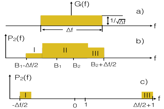
Figure 3: a) The initial pointer’s state $G(f)$ in Eq.(13); b) Probability distribution of the pointer’s readings, $W(f)=|\Psi(f)|^{2}$, for a system found in $|c_{2}{\rangle}$ at $t=t_{2}$ (schematic, arbitrary units). If a reading $f$ lies in regions $I$ or $II$, Bob knows that ${\hat{B}}$’s value was $B_{1}$ or $B_{2}$, respectively. Nothing can be said about the value of ${\hat{B}}$ if the reading lies in the region II. c) A projector ${\hat{B}}=|b_{2}{\rangle}{\langle}b_{2}|$ with the eigenvalues $0$ and $1$ is measured by a weakly coupled pointer, $\Delta f>>1$, in the case that the transition is forbidden, $A(c_{2}\leftarrow b_{1}\leftarrow a_{1})=-{\mathcal{A}}(c_{2}\leftarrow b_{2}\leftarrow a_{1})$. The readings are unusually large, $|f|>>1$, and Alice always knows the value of ${\hat{B}}$ at $t=t_{2}$.

The pointer becomes more accurate as $\Delta f\to 0$, and $|G(f)|^{2}\to\delta(f)$, in which case each trial yields either $f=B_{1}$ or $f=B_{2}$. For an inaccurate pointer, $\Delta f>|B_{2}-B_{1}|/2$, there is a region where the two $G$’s in (12) overlap (see Fig.3b). If Bob finds a reading $f$ inside that region, he can say nothing about the value of ${\hat{B}}$ (cf. subsection A). Otherwise he knows the path chosen by the system. As in the Feynman’s example, the probability to find the system in a state $|c_{n}{\rangle}$ at $t=t_{2}$ is a weighed sum

$$W_{n}=\beta W_{n}(\text{no\;interference})+(1-\beta)W_{n}(\text{interference}),\quad(n=1,2),$$ (14)

where $\beta=2|B_{2}-B_{1}|/\Delta f$, and $W_{n}(\text{interference})$ and $W_{n}(\text{no\;interference})$ are given by Eqs.(9) and (10), respectively. Note that sending $\Delta f\to\infty$ is equivalent to introducing a new scaled variable $f^{\prime}=f/\Delta f$, which changed the coupling Hamiltonian to $\hat{H}_{int}=-i{\hat{B}}\delta(t-t_{1})/\Delta f\;\partial_{f^{\prime}}$. Broadening $G(f)$ is, therefore, equivalent to reducing the coupling between the system and the pointer.
It is instructive to see what happens in the case of a previously forbidden transition (Fig. 3c), where ${\mathcal{A}}(c_{2}\leftarrow b_{1}\leftarrow a_{1})=-{\mathcal{A}}(c_{2}\leftarrow b_{2}\leftarrow a_{1})\equiv{\mathcal{A}}$, and Bob measures a projector ${\hat{B}}=|b_{2}{\rangle}{\langle}b_{2}|$. For $\Delta f>|B_{2}-B_{1}|$, $f$ may now lie in one of the intervals $[-\Delta f/2,-\Delta f/2+1]$ or $[\Delta f/2,\Delta f/2+1]$, and in each case Bob knows that ${\hat{B}}$ had either a value $0$ (the system was in $|b_{1}{\rangle}$), or $1$ (the system was in $|b_{2}{\rangle}$). The system reaches $|c_{2}{\rangle}$ with a probability $2|{\mathcal{A}}|^{2}/\Delta f<<1$, as the pointer has modified destructive interference between the paths, allowing it to reach, on a few occasions, the previously inaccessible final destination. For $\Delta f>>1$ , Bob needs to wait a long time for an arrival in $|c_{2}{\rangle}$, but in each such arrival the pointer’s displacement is very large, $\sim\pm\Delta f/2$. Note that this happens not because the pointer has experienced an unusually large shift, but because it could be found not far from there even before the measurement was made.

IV.4 Fuzzy detections

Thus, continues Feynman FeynL , the way to observe the particles without disturbing them considerably may be to increase the photon’s wavelength, rather than decrease their number. A red coloured photon carries a smaller momentum than a blue one, so the jolt produced on the particle should also be smaller. However, if the wavelength $\lambda$ were to exceed the distance between the slits, $d$, one would only see a “fuzzy” flash, unable to decide which of the two slits it came from. This is another illustration of the Uncertainty Principle (f): “an apparatus, capable of determining which way a particle goes, cannot be so delicate so as not to disturb the interference pattern in an essential way FeynL .”
Such a fuzzy detection can be mimicked by using a pointer prepared in a Gaussian (rather that in a rectangular) state,

$$G(f,\Delta f)=\left(\pi\Delta f^{2}/2\right)^{-1/4}e^{-f^{2}/\Delta f^{2}},$$ (15)

where $\Delta f$ exceeds the difference of the measured values, and the condition $\lambda>d$ is replaced by $\Delta f>|B_{2}-B_{1}|$.
Consider again the situation where one measures an operators ${\hat{B}}=|b_{1}{\rangle}{\langle}b_{1}|$. The probability of finding a reading $f$, conditional on post-selection in $|c_{2}{\rangle}$, is given by

$$W(f)=|G(f-1){\mathcal{A}}(c_{2}\leftarrow b_{1}\leftarrow a_{1})|^{2}+|G(f)|{\mathcal{A}}(c_{2}\leftarrow b_{2}\leftarrow a_{1})|^{2}+$$ (16)

$$2\text{Re}[G(f-1)G(f){\mathcal{A}}^{*}(c_{2}\leftarrow b_{1}\leftarrow a_{1}){\mathcal{A}}(c_{2}\leftarrow b_{1}\leftarrow a_{1})].\quad\quad$$

Even though there are two scenarios the system may follow, the last interference term clearly prevents one from knowing which of them has actually been realised if the measurement is fuzzy. The term disappears if the measurement is sharp $\Delta f<<|B_{2}-B_{1}|$, and the system is always seen to choose one of the two paths.
One might object by pointing out that we kept changing the subject. By sending $\Delta f\to 0$ Bob perturbs the system considerably, while one only wished to know what happened to the unperturbed system. There is an orthodox answer to that too. The wish cannot be granted, or the Uncertainty Principle (f), necessary for the very existence of the quantum theory FeynL , would be violated. It appears that the “which way?” question simply cannot be answered in the presence of interference.
We could finish the discussion with the adaptation of the general rules of FeynL to the needs of the measurement theory, were it not for one additional circumstance.

V The “Weak measurements”

In an attempt to study the properties of an (almost) unperturbed system, Alice may send $\Delta f$ in Eq.(15) to infinity. The first thing she would notice is that if the final position of the pointer is representative of the value of the measured ${\hat{B}}$, this value is, indeed, indeterminate, since $f$ can lie almost anywhere. The answer to a question which should have no answer can be “anything at all”. She can also expect that no other useful information can be extracted from the very broad distribution of the pointer’s reading. It is only reasonably to expect that the final mean reading of an infinitely inaccurate pointer would also be zero, just as was the initial one.
This is, however, not the case. In SPIN100 the authors have shown (using a different language and notations) that the average pointer’s reading in the limit $\Delta f\to\infty$ is given by

$${\langle}f{\rangle}\equiv\frac{\int f|\Psi(f)|^{2}df}{\int|\Psi(f)|^{2}df}{\xrightarrow[\Delta f\to\infty]{}}\text{Re}\left[\sum_{l}B_{l}\alpha_{l}\right]\equiv\text{Re}[{\langle}{\hat{B}}{\rangle}_{W}],$$ (17)

where

$$\alpha_{l}=\frac{{\mathcal{A}}(c_{2}\leftarrow b_{l}\leftarrow a_{1})}{\sum_{l^{\prime}}{\mathcal{A}}(c_{2}\leftarrow b_{l}^{\prime}\leftarrow a_{1})}$$ (18)

is the path amplitude, renormalised to a unit sum over the paths leading to the same destination $|c_{2}{\rangle}$, $\sum_{l}\alpha_{l}=1$. The complex valued quantity ${\langle}{\hat{B}}{\rangle}_{W}$ was called “the weak value (WV) of ${\hat{B}}$”. Its imaginary part, $\text{Im}[{\langle}{\hat{B}}{\rangle}_{W}]$, can be obtained if the pointer’s mean final momentum is measured instead SPIN100 , (see also DSpla1 ). In practice this means that after repeating his measurements $K>>1$ times, Bob will be able to deduce the value in the r.h.s. of Eq.(17) sufficiently accurately, even if the uncertainty of each trial, $\Delta f$, is as large as he wants, and the interference between the system’s paths is affected as little as he wants. [Bob’s task, although possible in principle, will rapidly become impractical. Indeed, by the Central Limit Theorem CLT , the number of trials (copies of the system) will have to grow as $K\sim\Delta f^{2}/\text{Re}[{\langle}{\hat{B}}{\rangle}_{W}]^{2}$. ]
This result should be of interest to anyone wishing to challenge the conclusions of Refs. FeynL , FeynC , and FeynH . Contrary to one’s expectations, a concrete information clearly related to the intermediate condition of an (almost) unperturbed system can be obtained experimentally. Does measuring ${\langle}f{\rangle}$ in this manner allow Bob to speak about the things Feynman thought unspeakable?

V.1 “Weak values” and the Uncertainty Principle

Apparently not. The Uncertainty Principle of FeynL does not forbid knowing the values of the probability amplitudes. It does, however, forbid to make assumptions about the system’s past where the scenarios one wishes to distinguish continue to interfere. Nothing in the Principle stops Bob from learning the values of either the amplitudes (18), or of their various combinations (17). The question is, what conclusions is he allowed to draw from the “weak values” once they have been measured?
Before addressing it, it may be useful to demonstrate that there always exists a transition in which the weak value of any chosen operator ${\hat{B}}$ equals any desired complex number $Z$. Indeed, there are infinitely many choices of $\alpha_{l}={\mathcal{A}}_{l}/\sum_{l^{\prime}}{\mathcal{A}}_{l^{\prime}}$, such that ${\langle}{\hat{B}}{\rangle}_{W}=\sum_{\ell}B_{l}\alpha_{l}$ equals $Z$. If a particular set $\alpha_{i}(Z)$ has been chosen, the path amplitudes ${\mathcal{A}}_{l}$ must satisfy

$$\sum_{l^{\prime}=1}^{N}[S_{ll^{\prime}}-\delta_{ll^{\prime}}]{\mathcal{A}}_{l^{\prime}}=0,\quad(S_{ll^{\prime}}\equiv\alpha_{l}\quad\text{for all}\quad l^{\prime}).$$ (19)

Since $\sum_{l=1}^{N}\alpha_{l}=1$, the matrix in the square brackets is degenerate, and the system (19) has a particular solution ${\mathcal{A}}_{l}=\alpha_{l}/\alpha_{1}$.
If only three quantities are measured, the amplitudes are given by

$${\mathcal{A}}_{l}={\langle}c_{n}|\hat{U}^{S}(t_{2},t_{1})|b_{l}{\rangle}{\langle}b_{l}|\hat{U}^{S}(t_{1},t_{0})|a_{k}{\rangle}\equiv{\langle}b_{l}|c_{n}(t_{1}){\rangle}^{*}{\langle}b_{l}|a_{k}(t_{1}){\rangle},$$ (20)

and for any $|a_{k}{\rangle}$ one finds a (yet unnormalised) state $|c_{n}(t_{1}){\rangle}$, ${\langle}b_{l}|c_{n}(t_{1}){\rangle}=\alpha_{l}^{*}/[\alpha_{1}{\langle}b_{l}|a_{k}(t_{1}){\rangle}]^{*}$. Normalising $|c_{n}{\rangle}$ to unity yields a final state $|c_{n}{\rangle}$ such that, for a given initial state $|a_{k}{\rangle}$, ${\langle}{\hat{B}}{\rangle}_{W}$ equals the desired value $Z$,

$$|c_{n}{\rangle}=\hat{U}^{S}(t_{2},t_{1})|c_{n}(t_{1}){\rangle},\quad{\langle}b_{l}|c_{n}(t_{1}){\rangle}=\frac{\alpha_{l}^{*}(Z)}{{\langle}b_{l}|\hat{U}^{S}(t_{1},t_{0})|a_{k}{\rangle}}\left[\sum_{l^{\prime}=1}^{N}\frac{|\alpha_{l^{\prime}}(Z)|^{2}}{|{\langle}b_{l^{\prime}}|\hat{U}^{S}(t_{1},t_{0})|a_{k}{\rangle}|^{2}}\right]^{-1/2}.\quad$$ (21)

The indeterminacy implied by the Uncertainty Principle is restored, albeit at a higher level, where all possible transitions are considered. The weak value of a $z$-component of a spin-$1/2$ can be found to have a value ${\langle}\hat{\sigma}_{z}{\rangle}_{W}=1/2$, as well as ${\langle}\hat{\sigma}_{z}{\rangle}_{W}=1.2345*10^{19}-6.789*10^{28}i$. Both results are equally meaningful or, if one prefers, equally meaningless, as we discuss next.

V.2 Interpretation of the “weak values”

This is the most contentious part of our discussion. Enter Carol who, unlike Alice, suspects that Feynman’s narrative FeynL it too restrictive, and there is more to be learnt through the “weak measurements” described above.
C: You forbid saying anything about the value of ${\hat{B}}$ half way through the transition. I put it to you that this weak (WV) value is given by Eq.(17). The authors of SPIN100 have shown that Bob can measure a component of a spin-$1/2$ and give you a number $100$. Here is the answer to a question which you thought could have no answer.
A: By the same logic, the WV of a projector ${\hat{B}}=|b_{1}{\rangle}{\langle}b_{1}|$ should be the probability of the system taking that path. I can always find a transition [cf. Eq.(21)] where ${\langle}{\hat{B}}{\rangle}_{W}=-5i$. This is not a probability. A probability is related to the number of occurrences, and always has value between $0$ and $1$. I do, however, have a different name for this result: it is a probability amplitude (18).
C: All right, one cannot substitute the relative amplitudes for probabilities, but maybe they be interpreted as “occupation numbers”, as was suggested in OCCUP . Let us say that the “weak value” of a projector ${\hat{B}}=|b_{l}{\rangle}{\langle}b_{l}|$, ${\langle}{\hat{B}}{\rangle}_{W}=\alpha_{l}$, represents, in some sense, the “number of particles” in the $l$-th path (the $l$-th arm of an interferometer, if an optical realisation of the experiment is considered). These weak values can be measured simultaneously, obey a “self-consistent logic”, and should lead to a “deeper understanding of the nature of quantum mechanics” according to OCCUP .
A: I am afraid, you would have the same problem: $-5i$ is by no stretch of imagination a valid number of particles (or particle pairs as proposed in OCCUP ). It would be even worse for a “dark” final state, where $\sum_{l}{\mathcal{A}}(c_{2}\leftarrow b_{l}\leftarrow a_{1})=0$, unless you want to tell Bob that infinitely many particles in each pathway conspire so that nothing arrives at the final destination $|c_{2}{\rangle}$. Besides, a WV of a projector is not a good local indicator, and should not be used to quantify what happens in a particular arm of the interferometer (see Appendix A). The WV of ${\hat{B}}=|b_{l}{\rangle}{\langle}b_{l}|$ depends on the amplitudes of all pathways leading to the same final state [cf. Eq.(49)], in a way its accurate “strong” value does not [cf. Eq.(47)]. And, by the way, the “self-consistent logic” OCCUP enjoyed by the weak values is but the property that the relative amplitudes (18) always add up to unity.
C: Let us forget about the numerical values of the WVs, be they real or imaginary, and simply use them as indicators of the particle’s presence in particular part of the system, as was suggested in PHOT2 . One couples a weak pointer to a particular system’s state (or a part of the interferometer). Surely, if the pointer does not move (the weak value of the corresponding projector is $0$), the system never visits that part of the Hilbert space? If, on the other hand, it did move, the system must have been there. What can possibly go wrong with relying on such a “weak trace”?
A: This is the same as saying that the system does not use a pathway whose amplitude is zero. But the pathways can be combined, and you will be in danger of finding the particle in parts while no finding it in the whole. This is not too different from Feynman’s dilemma of Sect.3A, whereby one finds more particles arriving at the screen if one slit is closed. We will discuss this case next.

VI The three-slit case.

With three rather than just two dimensions it comes a possibility of measuring operators with degenerate eigenvalues, which we will explore next. There are now three paths, connecting $|a_{1}{\rangle}$ with $|c_{1}{\rangle}$, which, to shorten the notations, we will denote $\{l\}\equiv\{c_{1}\leftarrow b_{l}\leftarrow a_{1}\}$, and three amplitudes, ${\mathcal{A}}_{l}\equiv{\mathcal{A}}(c_{1}\leftarrow b_{l}\leftarrow a_{1})$, $l=1,2,3$ (see Fig.4a). We will consider two commuting projectors,

$${\hat{B}}=|b_{1}{\rangle}{\langle}b_{1}|,\quad\quad\quad\quad\quad B_{1}=1,\quad B_{2}=B_{3}=0,\quad\quad\quad\quad$$ (22)

$${\hat{B}}^{\prime}=|b_{1}{\rangle}{\langle}b_{1}|+|b_{2}{\rangle}{\langle}b_{2}|,\quad B^{\prime}_{1}=B^{\prime}_{2}=1,\quad B^{\prime}_{3}=0,\quad\quad\quad\quad$$

designed to question the presence of the system, at $t=t_{1}$, in the state $|b_{1}{\rangle}$, and in the sub-space spanned by $|b_{1}{\rangle}$ and $|b_{2}{\rangle}$, respectively. Following 3BOX , we tune the system to ensure

$${\mathcal{A}}_{1}=-{\mathcal{A}}_{2}={\mathcal{A}}_{3}\equiv A,\quad\quad(\alpha_{1}=-\alpha_{2}=\alpha_{3}=1).$$ (23)

If no measurements are made, the probability of the system arriving at $|c_{1}{\rangle}$ at $t=t_{2}$ is $W_{1}=\left|\sum_{l=1}^{3}A_{l}\right|^{2}=|A|^{2}$.

VI.1 No paradox so far

An accurate measurement of ${\hat{B}}$ always finds the system in the state $|b_{1}{\rangle}$ (we omit the dependence on $|a_{1}{\rangle}$ and $|c_{1}{\rangle}$)

$$P(B=1)=|{\mathcal{A}}_{1}|^{2}/(|{\mathcal{A}}_{1}|^{2}+|{\mathcal{A}}_{2}+{\mathcal{A}}_{3}|^{2})=1.$$ (24)

However, an accurate measurement of ${\hat{B}}^{\prime}$ never finds it in the sub-space containing $|b_{1}{\rangle}$,

$$P(B^{\prime}=1)=|{\mathcal{A}}_{1}+{\mathcal{A}}_{2}|^{2}/(|{\mathcal{A}}_{1}+{\mathcal{A}}_{2}|^{2}+|{\mathcal{A}}_{3}|^{2})=0.$$ (25)

In both cases the probability of a successful post-selection in $|c_{1}{\rangle}$ is, as before, $W_{1}=|A|^{2}$. Although the authors of 3BOX found this “paradoxical”, there is nothing particularly surprising. In Sect. II we went to some length stressing the need for employing a probe which would carry the record of the outcome obtained at $t=t_{1}$ until the experiment is finished just after $t_{2}$. Measuring ${\hat{B}}$ and ${\hat{B}}^{\prime}$ requires different probes ($-i\partial_{f}{\hat{B}}\neq-i\partial_{f}{\hat{B}}^{\prime}$) which affect the system, expected later to reach the same final state, in different ways. The resulting statistical ensembles are, therefore, different, and there is no conflict between Eqs.(24) and (25) DSpath .
Measuring ${\hat{B}}$ and ${\hat{B}}^{\prime}$ one after another also shows nothing unusual. With two intermediate measurements there are $9$ paths, of which only three have non-zero amplitude (we put $\hat{H}^{S}=0$)

$${\mathcal{A}}(c_{1}\leftarrow b_{l^{\prime}}\leftarrow b_{l}\leftarrow a_{1})={\langle}c_{1}|b_{l^{\prime}}{\rangle}{\langle}b_{l^{\prime}}|b_{l}{\rangle}{\langle}b_{l}|a_{1}{\rangle}=A\delta_{ll^{\prime}}.$$ (26)

There are also four possible outcomes, $B=0,1$, $B^{\prime}=0,1$. The outcome $(B=1,B^{\prime}=0)$ would indeed be problematic, indicating the presence of the system in the path $1$ but not in the union of the paths $1$ and $2$. However, this scenario is never realised, as the corresponding probability vanishes, $P(B=1,B^{\prime}=0)=0$ (see Fig.4b). Each of the three remaining outcomes allow to identify the paths taken by the system, and by (c) of Sect. III, one has

$$P(0,0)=P(0,1)=P(1,1)=|A|^{2}/(|A|^{2}+|-A|^{2}+|A|^{2})=1/3.$$ (27)

We note also that, just like in Feynman’s two-slit example of Sect.4A, determination of the path taken by the system increases the odds on its arriving in the state $|c_{1}{\rangle}$, $W_{1}=\sum_{l=1}^{3}\left|A_{l}\right|^{2}=3|A|^{2}$. One cannot, therefore, say that an unobserved system is in one of the states $|b_{l}{\rangle}$, and not in the other two. By the same token, whenever some of the paths are not resolved by a measurement (the paths $\{1\}$ and $\{2\}$ in our example), it should be impossible to say that the system chooses one of them and not the other [cf. Eqs.(24) and (25)]. Next, as promised, we will bring the “weak values” into the discussion.

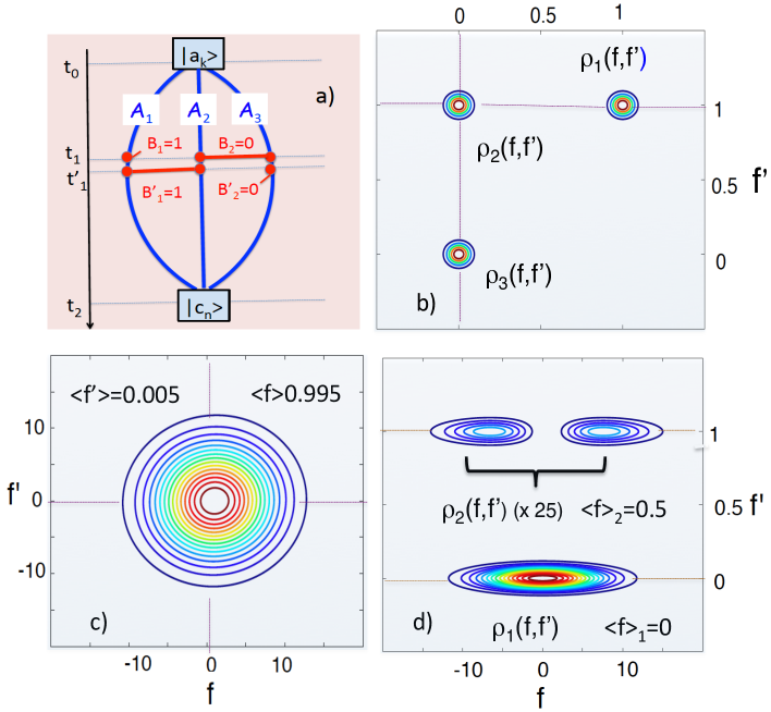
Figure 4: a) Three virtual pathways with the amplitudes ${\mathcal{A}}_{1}=-{\mathcal{A}}_{2}={\mathcal{A}}_{3}$. At $t=t_{1}$ Bob measures the operator ${\hat{B}}$ in Eq.(22), and at $t=t_{1}^{\prime}$, immediately after, the operator ${\hat{B}}^{\prime}$. What happens depends on the accuracy of Bob’s pointers. b) The distribution of the pointer readings, $\rho(f,f^{\prime})$ when both pointers are accurate (strong), $\Delta f=\Delta f^{\prime}=0.1$. c) The same distribution when both pointers are inaccurate (weak), $\Delta f=\Delta f^{\prime}=10$. d). The first pointer is accurate, $\Delta f=0.1$, and the second one is weak, $\Delta f^{\prime}=10$.

VI.2 An unlikely “cat”

To add panache to the story, we will refer to the system as a “cat”, promote the paths $\{1\}$ and $\{2\}$ to a “one-bedroom flat”, and call the remaining pathway $\{3\}$ the “yard”. Our aim, we recall, is to divine the behaviour of an unobserved and, therefore, unperturbed cat. To do so we will relay on the existence or absence of the “weak traces”, non-zero “weak values” of the corresponding projectors. Using Eq.(23) we find that the weak pointer looking for the cat in the bedroom $\{1\}$ has indeed “moved”,

$${\langle}{\hat{B}}{\rangle}_{W}=B_{1}\alpha_{1}+B_{2}(\alpha_{2}+\alpha_{3})=1\neq 0.$$ (28)

The weak pointer looking for it in the entire flat, however, did not (see Fig.4c)

$${\langle}{\hat{B}}^{\prime}{\rangle}_{W}=B^{\prime}_{1}(\alpha_{1}+\alpha_{2})+B_{3}\alpha_{3}=0,$$ (29)

and we have a “paradox”: A quantum cat can be in a part of the flat, and yet not in the flat as a whole.
This puzzle is, however, not entirely our own. A similar “paradox” was described in PHOT2 , where three successive WMs yielding ${\langle}{\hat{B}}^{\prime}{\rangle}_{W}=0$, ${\langle}{\hat{B}}{\rangle}_{W}\neq 0$ and again ${\langle}{\hat{B}}^{\prime}{\rangle}_{W}=0$ gave the impression that a quantum system can suddenly appear in a the state $|b_{1}{\rangle}$, without being there immediately before and immediately after. An optical realisation of the experiment led the authors of PHOT2 to conclude that “the past of the photons is not represented by continuous trajectories”. Next we ask whether a similar interpretation of the results (28) and (29) can lead Bob to a wrong prediction.

VII The three-slit case. How to make a wrong prediction

Bob the practitioner is duly surprised, and wants to make further predictions based on the cat’s strange behaviour. He may be thinking: the weak pointer measuring ${\hat{B}}^{\prime}$ “has not moved”, ${\langle}{\hat{B}}^{\prime}{\rangle}_{W}=0$, because it has not interacted with the cat, who is absent from the flat. Surely, if the cat is really absent, a closer look inside the flat would not affect it at all. Thus, a more accurate measurement of ${\hat{B}}^{\prime}$ should not change anything for the weak pointer measuring ${\hat{B}}$. Bob improves the accuracy of the second measurement by sending $\Delta f^{\prime}\to 0$, leaves the measurement of ${\hat{B}}$ “weak”, and expects still to find the trace of the cat in the bedroom $\{1\}$.
This is, however, not what he finds. Bob’s accurate measurements of ${\hat{B}}^{\prime}$ have created two “real” (as opposed to “virtual”) scenarios for the system. It can reach the final state $|c_{1}{\rangle}$ via the path $\{3\}$, with a probability $|{\mathcal{A}}_{3}|^{2}$. Alternatively it can reach it via a scenario in which the paths $\{1\}$ and $\{2\}$, not resolved by the first Bob’s measurement of ${\hat{B}}$, continue to interfere. The second possibility is a double-slit problem in its own right, and a one in which virtual paths lead to a “dark fringe”, since ${\mathcal{A}}_{1}=-{\mathcal{A}}_{2}$. The probability of taking this route is, therefore, zero, $|{\mathcal{A}}_{1}+{\mathcal{A}}_{2}|^{2}=0$. The mean reading of the weak pointer measuring ${\hat{B}}$, conditional on finding the system in $|c_{1}{\rangle}$, is

$${\langle}f{\rangle}=\frac{\text{Re}\left[\frac{B_{1}{\mathcal{A}}_{1}+B_{2}{\mathcal{A}}_{2}}{{\mathcal{A}}_{1}+{\mathcal{A}}_{2}}\right]|{\mathcal{A}}_{1}+{\mathcal{A}}_{2}|^{2}+B_{3}|{\mathcal{A}}_{3}|^{2}}{|{\mathcal{A}}_{1}+{\mathcal{A}}_{2}|^{2}+|{\mathcal{A}}_{3}|^{2}}=0,$$ (30)

so there is no cat in the flat, no longer a “weak trace” of the cat in the bedroom and, therefore, no paradox.
To see how the result (30) is obtained, consider a measurement of ${\hat{B}}^{\prime}$ to a good, yet finite accuracy, $0<\Delta f^{\prime}<<1$ Bob’s results are shown in Fig. 4d. The probability distribution of the readings consists of two disjoint parts, $\rho(f,f^{\prime})=[\omega_{1}+\omega_{2}]/\int(\omega_{1}+\omega_{2})dfdf^{\prime}\equiv\rho_{1}+\rho_{2}$ (see Appendix B) where

$$\omega_{1}(f,f^{\prime})=|G(f,\Delta f)|^{2}|G(f^{\prime},\Delta f^{\prime})|^{2}|{\mathcal{A}}|^{2},\quad\quad\quad\quad\quad\quad\quad\quad\quad\quad$$ (31)

$$\omega_{2}(f,f^{\prime})=|G(f-1,\Delta f^{\prime})-G(f,\Delta f^{\prime})|^{2}|G(f^{\prime}-1,\Delta f^{\prime})|^{2}|{\mathcal{A}}|^{2}|.$$

The first part corresponds to the cat not found in the flat, and shows no trace of the cat in the bedroom, ${\langle}f{\rangle}_{1}=\int f\rho_{1}(f,f^{\prime})dfdf^{\prime}=0$. The second part finds the cat in the flat, and there is also a trace of it in the bedroom (the meters are Gaussian), ${\langle}f{\rangle}_{2}=\int f\rho_{1}(f,f^{\prime})dfdf^{\prime}{\xrightarrow[\Delta f\to\infty]{}}1/2$. However, the probability of the latter outcome, which occurs only because the second Bob’s pointer slightly upsets otherwise perfect cancellation between the paths $\{1\}$ and $\{2\}$, vanishes as $\Delta f\to\infty$ $\int\rho_{2}(f,f^{\prime})dfdf^{\prime}\sim 1/\Delta f^{2}{\xrightarrow[\Delta f\to\infty]{}}0$ (see Appendix B), and Bob only gets the outcomes where neither of the two pointers “has moved”.
Alice and Carol again:

C: A quantum system can be absent from a subspace of its Hilbert space, yet simultaneously present in a smaller part of that subspace. In an optical experiment a photon can be present in one arm of the interferometer, but absent from a larger part of the setup, containing the arm in question.
A: And how do you know that?
C: A weak pointer moves (albeit on average) if I look in a smaller subspace, but not if I look in the larger one.
A: Your “paradoxical” conclusion is predicated on the link between the movement of the pointer and the actual presence of the system at the specified location. But you can also look at your result differently. You are simply saying that the system is simultaneously present in all the pathways were the corresponding amplitudes, ${\mathcal{A}}_{l}$, does not vanish. If so, in a double-slit experiment a particle passes via both slits at the same time. In the orthodox view FeynL , FeynC , FeynH you can always say that an ${\color[rgb]{0,0,1}{\mathcal{A}}_{l}}\neq 0$. You cannot, however, conclude from this that the system, or a part of it, is there.
C: And why is that?
A: Because a more accurate measurement may find the entire system elsewhere, or destroy the “paradox” as was discussed in above example. Your prediction will be proven wrong.
C: But you said yourself that an accurate measurement will disturb the system, and I am taking about the experimental evidence of an unperturbed system’s behaviour. Perhaps the weak measurements, unknown to the authors of FeynL , FeynC , FeynH at the time, conveniently filled the gap left in their reasoning?
A: The authors of FeynL , FeynC , FeynH have an answer to this. The fact that one can deduce the values of the amplitudes experimentally is of no fundamental importance. The amplitudes are always known to a theorist, and the orthodox contention is that they cannot be used beyond what is covered by the rules of Sect. III. In FeynC , Feynman admits that one can say something about what happens to the system in the presence of interference, but needs “to stop thinking immediately and make no deductions from it”. You can say that there are particles passing through each slit yet never arriving at a dark fringe on the screen. You can say that photons have discontinuous trajectories PHOT2 , or that a cat both is and is not inside the flat, but that is all. “Physicists prefer not to say it , rather than stop thinking at the moment.” FeynC .

VIII The four-slit case. “Quantum Cheshire cats”

Adding the fourth dimension allows one to consider a pair of two-level systems. Following CAT1 call the first one a “Cheshire cat” (sic!), and the second one the cat’s “grin”. The cat can be either “on the right”, or “on the left”, i.e., in states $|L{\rangle}$ or $|R{\rangle}$, respectively. The grin can be “up” or “down”. The four possible states of the joint system, therefore, are

$$|b_{1}{\rangle}=|L{\rangle}|\text{up}{\rangle},\quad|b_{2}{\rangle}=|L{\rangle}|\text{down}{\rangle},\quad|b_{3}{\rangle}=|R{\rangle}|\text{up}{\rangle},\quad|b_{4}{\rangle}=|R{\rangle}|\text{down}{\rangle}.$$ (32)

There are also two operators, diagonal in the basis (32),
${\hat{B}}=|L{\rangle}{\langle}L|$, with the eigenvalues $(1,1,0,0)$, and
${\hat{B}}^{\prime}=|R{\rangle}{\langle}R|\otimes(|\text{up}{\rangle}{\langle}\text{up}|-|\text{down}{\rangle}{\langle}\text{down}|)$, with the eigenvalues $(0,0,1,-1)$,
where the operator $|\text{up}{\rangle}{\langle}\text{up}|-|\text{down}{\rangle}{\langle}\text{down}|$, akin to the $z$-component of a spin-$1/2$, $\hat{\sigma}_{z}$, represents the “cat’s” “grin”. One can always choose (see Sect. VA) the four amplitudes ${\mathcal{A}}_{l}\equiv{\mathcal{A}}(c_{n}\leftarrow b_{l}\leftarrow a_{k})$, $l=1,2,3,4$ as

$${\mathcal{A}}_{1}=-{\mathcal{A}}_{2}={\mathcal{A}}_{3}={\mathcal{A}}_{4},\quad(\alpha_{1}=-\alpha_{2}=\alpha_{3}=\alpha_{4}=1/2).$$ (33)

We leave it to the reader to check what happens if the above operators are measured accurately, together or separately, and note only that the “weak values” of both operators vanish,

$${\langle}{\hat{B}}{\rangle}_{W}=0,\quad{\langle}{\hat{B}}^{\prime}{\rangle}_{W}=0.$$ (34)

To follow the story one has (a) to agree that a null “weak value” of ${\hat{B}}$ means that the cat is not on the left , and (b) to accept that a null “weak value” of ${\hat{B}}^{\prime}$ means that the cat’s grin is not on the right. There is also a tacit assumption that if something is not in one place, it must be in the other, since neither the cat nor the grin are expected to disappear. Thus, one may conclude that the cat (on the right) has been “separated” from its grin (on the left), and consider other possible “separations” mentioned in the second of our epigraphs. Further discussion of this “paradox” can be found in CAT1 ,CAT2 .
Our purpose is to question the principle. In Eq.(34) ${\langle}{\hat{B}}{\rangle}_{W}$ vanishes because $B_{1}=B_{2}$ and ${\mathcal{A}}_{1}=-{\mathcal{A}}_{2}$. This situation was considered in some detail in the previous two Sections. The case of ${\langle}{\hat{B}}^{\prime}{\rangle}_{W}=0$ is slightly different. Now the path amplitudes are the same, ${\mathcal{A}}_{3}={\mathcal{A}}_{2}$, but the two eigenvalues have opposite signs, $B^{\prime}_{3}=-B^{\prime}_{4}$.
To clarify the situation, Bob (aware of Carol’s objections to using strong measurements) may decide to add yet another “weak” pointer, measuring ${\hat{B}}^{\prime\prime}=|L{\rangle}{\langle}L|\otimes|\text{up}{\rangle}{\langle}\text{up}|$. Whoever agrees with (a) and (b) must also accept that ${\langle}{\hat{B}}^{\prime\prime}{\rangle}_{W}$ indicates the presence of an “upwards grinning” cat at the left location. Having been told that there is no cat on the left, Bob expects to obtain ${\langle}{\hat{B}}^{\prime\prime}{\rangle}_{W}=0$, but finds instead ${\langle}{\hat{B}}^{\prime}{\rangle}_{W}=1/2$. Similarly, weakly measuring ${\hat{B}}^{\prime\prime\prime}=|R{\rangle}{\langle}R|\otimes|\text{up}{\rangle}{\langle}\text{up}|$, he finds the “up” component of the grin on the right, since ${\langle}{\hat{B}}^{\prime\prime\prime}{\rangle}_{W}$ is also $1/2$.
The story “told by the simultaneous weak values” is now as follows:

(i) there is no cat on the left hand side of the setup,

(ii) yet there is a cat there, provided its grin is “up”,

(iii) there is no grin on the right hand side,

(iv) yet there is a grin, provided it is “up”.
Alice and Carol again.
A: You told Bob that there is no grin on the right hand side, but he finds a part of it there. Another wrong prediction?
C: Au contraire, you just discovered another quantum mechanical paradox: Bob can have the cat in one place, the cat’s grin elsewhere, and still a bit of the grin where the grin is not. Have you two thought of a publication?
A: All we know is that Bob’s “weak measurements” have confirmed the relations (33) between the four amplitudes in question. But there is no surprise, Bob has set up his experiment ensuring that $\alpha_{1}=-\alpha_{2}=\alpha_{3}=\alpha_{4}$. Your “paradox” disappears the moment you stop interpreting Eqs.(33) the way you do.
C: And how should I interpret them?
A: You should not interpret them at all, lest you create spurious “paradoxes”.
C: What if I like paradoxes?
The next Section contains our conclusions.

IX Conclusions and discussion

In summary, our aim was compare two apparently contradictory approaches to the description of quantum behaviour. The first one, which we called the orthodox, can be applied to quantum measurements as follows. An experimentalist wants to measure three (or more) quantities one after another. He/she needs probes (pointers) to read off the past measured values at the end of experiment. A theorist describes the system in terms of virtual paths connecting the states in the system’s Hilbert space $\mathcal{H}_{S}$, and the corresponding probability amplitudes ${\mathcal{A}}_{l}$. If the equipment allows to determine the path taken by the system in each trial, absolute squares of the amplitudes, $|{\mathcal{A}}_{l}|^{2}$, predict the relative frequency (probability) with which a particular path will occur after many trials. A quantity $\bf B$ is represented by an operator ${\hat{B}}$ acting in $\mathcal{H}_{S}$. Its mean value, ${\langle}B{\rangle}$, is then obtained by multiplying each path probability by the corresponding eigenvalue of the operator ${\hat{B}}$, adding up the results, and normalising the sum as appropriate.
If the paths taken cannot be told apart, the amplitudes must be added, and one can neither say that a particular scenario was realised, nor that all the scenarios were realised at the same time. According to FeynL , FeynC , FeynH , either assumption about the system’s past would lead to wrong predictions, or contradictions. In particular, not even the mean value of $\bf B$ can be determined at a time between two observations. Moreover, there is no deeper explanation of the law of adding amplitudes, which must be accepted with all restrictions it imposes upon what can be known. These restrictions amounts to the Uncertainty Principle, a centrepiece of quantum description, without which “quantum mechanics would collapse” FeynL .
The Principle appears to leave an unpleasant void at the heart of the theory, and a desire to fill it can only be natural. The task is, however, difficult and, if attempted, must end either in an important new development, or in a misunderstanding of similar proportions. Feynman, for his part, was in no doubt that it would end in a “blind alley, from nobody has yet escaped” FeynC .
A different approach aims at describing a quantum system between measurements COMPL and, can, therefore, be seen as an attempt to fill the gap left by the Uncertainty Principle. For the purpose of our discussion it suffices to note that the method relies on experimentally accessible “weak value” (WV), ${\langle}B{\rangle}_{W}$, a sum of the probability amplitudes, weighted by the eigenvalues of the measured operator ${\hat{B}}$,

$${\langle}B{\rangle}_{W}=\sum_{l}B_{l}\alpha_{l},\quad\alpha_{l}=\frac{{\mathcal{A}}_{l}}{\sum_{l^{\prime}}{\mathcal{A}}_{l^{\prime}}}.$$ (35)

(more technical details are given in Appendix A). The amplitudes $\alpha_{l}$ are renormalised to a unit sum, and there always exists a transition, in which ${\langle}B{\rangle}_{W}$ takes any desired complex value (cf. Sect. V). As yet, there is no contradiction with the Uncertainty Principle which allows knowing probability amplitudes regardless of whether or not the system is being observed. It remains, however, to clarify the meaning of the result (35). Different propositions have been put forward by the authors of SPIN100 -CAT2 .
Could ${\langle}B{\rangle}_{W}$ yield the elusive value of $\bf B$ in the presence of interference? If so, one can have a component of a spin-$1/2$ equal to $100$ SPIN100 , a negative kinetic energy, a system “disembodied from its properties” CAT1 , a flux of “disembodied conserved properties” CAT2 , or a particle’s velocity exceeding the speed of light REL1 . The question is whether these results provide a further insight into the “machinery behind the law” FeynL . As always, the double slit case provides for a simple test. Let ${\hat{B}}$ measure the number of the slit chosen by the system, $B_{1}=1$ and $B_{2}=2$. Finding ${\langle}B{\rangle}_{W}=-100$, one must conclude that, with only two slits available, the system passes on average, through a slit number $-100$.
Could a WV be the “occupation number”, counting the number of particles, or particle-antiparticle pairs, as was suggested in OCCUP ? Again, in a double-slit experiment where two paths lead to a dark fringe, ${\mathcal{A}}_{1}=-{\mathcal{A}}_{2}$, the “occupation numbers” given by WV’s of the projectors ${\hat{B}}=|b_{1}{\rangle}{\langle}b_{1}|$ and ${\hat{B}}=|b_{2}{\rangle}{\langle}b_{2}|$ are $\infty$ and $-\infty$, respectively. The fact that the system never arrives in its final state appears to rely on the presence (in some strange sense) of infinitely many copies of the system in each of the paths leading to it.
Finally, and at first glance most reasonably, is simply to say that if the WV of a projector is $0$ (the weak pointer has not moved), the system has definitely not taken the chosen path PHOT2 , Matz1 . Conversely, if the pointer has moved, the system must have been present in the corresponding pathway. This is, however, the same as saying that the system is present, at the same time, in all pathways where the amplitudes ${\mathcal{A}}_{l}$ do not vanish. But, insisted the authors of FeynL , FeynC , FeynH , this would be a wrong conclusion. Besides, in the previous two-slit example, there will be be particles travelling towards a dark fringe via each of the slits, yet never arriving there at all. Similarly, in the three-slit example of Sects. VI and VII the system, this time arriving in its final state, can be “seen” in each of the two paths, yet conspicuously absent from their union.
The difference between the two approaches is now evident. None of the pictures just discussed serve as an explanation of the interference mechanism, as long as an explanation is expected to let one see a new phenomenon through a prism of accepted concepts. Rather, they look like a catalogue of illustrations of how an attempt to look inside the mechanism may end in the proverbial “blind alley” of FeynC .
There is, however, one more point to make. What could be said against using the “weak measurements” to portray the failures of classical concepts as novel “paradoxical” properties of the quantum world? There is an inexhaustible supply of such “paradoxes”, which can be displayed until the reader, or the editor, gets tired. To take a simple example, it is an experimental fact that in a double-slit experiment where $\alpha_{1},\alpha_{2}\neq 0$, the weak pointers, measuring projectors on each path, have both “moved”. Hence, in the quantum world, a system can be in two places at the same time 3BOX . In the orthodox view FeynL , FeynC , FeynH , this conclusion is wrong, since an additional measurement never finds parts of the system distributed between the pathways. To which an advocate of “weak measurements” can reasonably reply that he/she was referring to an unobserved system, and not to the one disturbed by this additional measurement. And if it is not in both places, then where was it? You can’t speak about this in the standard approach, replies the orthodox. And why is that? Because if I try to check your prediction, I only find it in one place. But I was referring to an unobserved system … at which point the conversation begins to circle. Apparently, Feynman has thought about this, since in FeynC he added: “ You can always say [that a particle goes through one hole or the other]- provided you stop thinking immediately and make no deductions from it. Physicists prefer not to say it, rather than stop thinking at the moment.” The same is true of other conclusions based on the “weak values”, or indeed on any approach relying on the probability amplitudes, rather than on the probabilities. One can say, for example, that the electron and its charge go different ways CAT1 , but the notion is so narrow that it is better not to say it at all. The barely speakable is, in practice, rather unspeakable.
Finally, it is remarkable the “weak measurements” approach, which purports “to revisit the whole quantum mechanical notion that physical variables are described by Hermitian operators” WV2010 has not, until now, been measured against the textbook orthodoxy of FeynL , FeynC , FeynH . Above we have tried to do just that, and even if the reader remains unconvinced by our arguments, he/she may be interested in revisiting the subject and drawing his/her own conclusions.

X Appendix A. Measurements: “Strong” and “weak”, Local and non-local.

Suppose Bob makes three measurements of $\hat{A}$, ${\hat{B}}$ and $\hat{C}$. Bob will use three von Neumann pointers vN with positions $f_{A}$, $f_{B}$, and $f_{C}$, prepared in the initials states

$$|D^{I}(0){\rangle}=\int G(f_{I},\Delta f_{I})|f_{I}{\rangle}df_{I},\quad I=A,B,C.$$ (36)

The functions $G(f_{I},\Delta f_{I})$, whether complex or real valued, have a property [$\delta(f)$ is the Dirac delta]

$$|G(f_{I},\Delta f_{I}\to 0)|^{2}\to\delta(f_{I}),$$ (37)

and become very broad and slow-varying as $\Delta f_{I}\to\infty$ . The pointers, which have no own dynamics, can be briefly coupled to the system by means of $\hat{H}^{int}_{I}=-i\partial_{f_{A}}\hat{I}\delta(t-t_{I})$, $t_{I}=t_{0},t_{1},t_{2}$, so that each interaction entangles a pointer with the system. For example, we have $\hat{U}^{int}_{B}(t)\equiv\exp[\int_{t_{1}-\epsilon}^{t_{1}+\epsilon}\hat{H}^{int}_{B}dt]=\sum_{l=1}^{N}|b_{l}{\rangle}{\langle}b_{l}|\exp(-i\partial_{f_{B}}B_{l})$, so that ($|\psi_{S}{\rangle}$ is an arbitrary system’s state)

$$|\hat{U}^{int}_{B}(t_{1})|D^{B}(0){\rangle}|\psi_{S}{\rangle}=\sum_{l=1}^{N}{\langle}b_{l}|\psi_{S}{\rangle}\left[\int G(f_{B}-B_{l},\Delta f_{B})|f_{B}{\rangle}df_{B}\right]|b_{l}{\rangle}$$ (38)

$$\equiv\sum_{l=1}^{N}{\langle}b_{l}|\psi_{S}{\rangle}|D^{B}(B_{l}){\rangle}|b_{l}{\rangle},$$

and similarly for the other two pointers.

X.1 Unitary evolution of the composite

At the end of his experiment Bob wants to know the likelihood of seeing particular pointer’s readings $f_{A}$, $f_{B}$ and $f_{C}$. Alice is only able to make the prediction, provided the first accurate measurement, $\Delta f_{A}\to 0$, prepares the composite $\{\it system\quad(S)+three\quad pointers\}$ in a known initial state

$$|\Phi(t_{0}){\rangle}=|D^{C}(0){\rangle}|D^{B}(0){\rangle}|D^{A}(A_{k}){\rangle}|a_{k}{\rangle}.$$ (39)

Note that the eigenvalue $A_{k}$ must not be degenerate. The composite undergoes unitary evolution until $t=t_{2}$, $|\Phi(t_{2}){\rangle}=\hat{U}^{S+Pointers}(t_{2},t_{1})|\Psi(t_{0}){\rangle}$, where

$$\hat{U}^{S+Pointers}(t_{2},t_{1})=\hat{U}^{int}_{C}(t_{2})\hat{U}_{S}(t_{2},t_{1})\hat{U}^{int}_{B}(t_{1})\hat{U}_{S}(t_{1},t_{0})$$ (40)

and $\hat{U}_{S}(t^{\prime},t)$ is the system’s evolution operator. It is readily seen that with $\hat{H}^{int}_{I}$ chosen as above,

$$|\Phi(t_{2}){\rangle}=\sum_{n=1}^{N}\sum_{l=1}^{N}{\mathcal{A}}(c_{n}\leftarrow b_{l}\leftarrow a_{k})|D^{C}(C_{n}){\rangle}|D^{B}(B_{l}){\rangle}|D^{A}(A_{k}){\rangle}|c_{n}{\rangle},$$ (41)

where ${\mathcal{A}}(c_{n}\leftarrow b_{l}\leftarrow a_{k})\equiv{\langle}c_{n}|\hat{U}^{S}(t_{2},t_{1})|b_{l}{\rangle}{\langle}b_{l}|)\hat{U}^{S}(t_{1},t_{0})|a_{k}{\rangle}$.
By (a) and (e) of Sect. III, there always exist probabilities of finding the composite in any one of the orthogonal states $|f_{C}{\rangle}|f_{B}{\rangle}|f_{A}{\rangle}|c_{n}{\rangle}$, $P(f_{C},f_{B},f_{A},c_{n})=|{\langle}f_{C}|{\langle}f_{B}|{\langle}f_{A}|{\langle}c_{n}|\Phi(t_{2}){\rangle}|^{2}$, which Alice needs to sum over the system’s states $|c_{n}{\rangle}$, in order to obtain the desired probability,

$$W(f_{C},f_{B},f_{A})=\sum_{n=1}^{N}P(f_{C},f_{B},f_{A},c_{n})=\quad\quad\quad\quad\quad\quad\quad\quad\quad$$ (42)

$$\sum_{n=1}^{N}\left|\sum_{l=1}^{N}{\mathcal{A}}^{S}(c_{n}\leftarrow b_{l}\leftarrow a_{k})G(f_{C}-C_{n})G(f_{B}-B_{l})G(f_{A}-A_{k})\right|^{2},$$

where $\hat{C}|c_{n}{\rangle}=C_{n}|c_{n}{\rangle}$, and $\int df_{A}df_{B}df_{C}W(f_{C},f_{B},f_{A})=1$.

X.2 Broken unitary evolution of the measured system

The pointers’ readings are only interesting insofar as they tell something about the measured system. Whatever can be learnt in this manner will, however, be expressed in terms of the transition amplitudes ${\mathcal{A}}^{S}(c_{n}\leftarrow b_{l}\leftarrow a_{k})$ corresponding to the system’s unitary evolution interrupted each times it interacts with one of the pointers. If the last measurement is also accurate, $\Delta f_{C}\to 0$, $G^{*}(f_{C}-C_{n^{\prime}})G(f_{C}-C_{n})=\delta(f-C_{n})\delta_{nn^{\prime}}$, Eq.(42) reduces to

$$W(f_{C},f_{B},f_{A})=\delta(f_{A}-A_{k})\sum_{n=1}^{N}\delta(f_{C}-C_{n})\left|\sum_{l=1}^{N}{\mathcal{A}}^{S}(c_{n}\leftarrow b_{l}\leftarrow a_{k})G(f_{B}-B_{l})\right|^{2}.$$ (43)

The probability of having at $t=t_{1}$ a reading $f_{B}$, while measuring $A_{k}$ and $C_{n}$ at $t=t_{0}$ and $t=t_{2}$, respectively, is, therefore, given by

$$W(C_{n},f_{B},A_{k})=\left|\sum_{l=1}^{N}{\mathcal{A}}^{S}(c_{n}\leftarrow b_{l}\leftarrow a_{k})G(f_{B}-B_{l})\right|^{2}\equiv\left|\sum_{l=1}^{N}{\mathcal{A}}_{l}(n)G(f_{B}-B_{l})\right|^{2}$$ (44)

(In the case of a degenerate eigenvalue $C_{m}$ one would need to sum Eq.(44) over all $|c_{n}{\rangle}$ corresponding to the same $C_{m}$.)
As an example, consider measuring at $t=t_{1}$ a projector ${\hat{B}}=|b_{2}{\rangle}{\langle}b_{2}|$ , with a non-degenerate eigenvalue $1$, and $(N-1)$-fold degenerate eigenvalue $0$. This is a double-slit problems with $N$ final states, sketched in Fig.5.

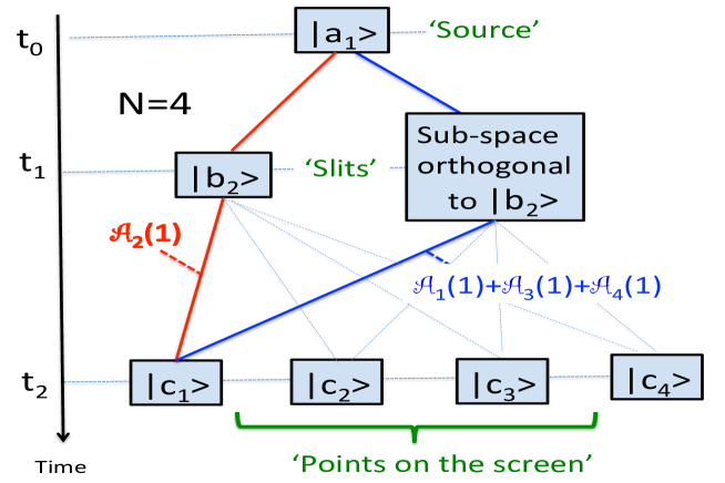
Figure 5: A “double-slit problem” arising from measuring a projector ${\hat{B}}=|b_{2}{\rangle}{\langle}b_{2}|$ in $N=4$ dimensions. There are two virtual routes to a final state $|c_{1}{\rangle}$, one passing through $|b_{2}{\rangle}$ at $t=t_{1}$, and the other not. The corresponding amplitudes are ${\mathcal{A}}_{2}(1)$ and $\sum_{l\neq 2}{\mathcal{A}}_{l}(1)$, respectively. [${\mathcal{A}}_{l}(n)\equiv{\langle}c_{n}|\hat{U}^{S}(t_{2},t_{1})|b_{l}{\rangle}{\langle}b_{l}|\hat{U}^{S}(t_{1},t_{0})|a_{1}{\rangle}$.] By measuring both ${\hat{B}}$ and $\hat{C}$ accurately, Bob can determine the route chosen by the system.

X.3 Accurate “strong” measurements and locality

If the second measurement is also accurate, $\Delta f_{B}\to 0$, there are only two possible readings, $f_{B}=1$ and $f_{B}=0$,

$$W(C_{n},f_{B},A_{k})\xrightarrow[f_{B}\to 0]{}|A_{2}(n)|^{2}\delta(f_{B}-1)+\left|\sum_{l\neq 2}{\mathcal{A}}_{l}(n)\right|^{2}\delta(f_{B}).$$ (45)

Notably the likelihood of the system being seen to take a path $\{c_{n}\leftarrow b_{2}\leftarrow a_{k}\}$ depends only on the corresponding amplitude, ${\mathcal{A}}^{S}(c_{n}\leftarrow b_{2}\leftarrow a_{k})$. This can be seen as a “local property”. In an optical realisation of the experiment, the probability of arriving at a detector via one arm of the interferometer would not depend on what happens elsewhere in the setup. This dependence does, however, appear if one calculates the relative probabilities of arriving at the same detector via different arms. Indeed, given that the system arrives in $|c_{n}{\rangle}$, for the frequency with which a path $\{c_{n}\leftarrow b_{2}\leftarrow a_{k}\}$ is chosen one has

$$P(c_{n}\leftarrow b_{2}\leftarrow a_{k})=\frac{|{\mathcal{A}}_{2}(n)|^{2}}{|{\mathcal{A}}_{2}(n)|^{2}+\left|\sum_{l\neq 2}{\mathcal{A}}_{l}(n)\right|^{2}}.$$ (46)

This is, however, still a “local” result since two probabilities in the denominator are evaluated separately for each of the routes shown in Fig.5. The same can be said about the mean pointer reading, also given by

$${\langle}f_{B}{\rangle}\equiv\frac{\int f_{B}W(C_{n},f_{B},A_{k})df_{B}}{\int W(C_{n},f_{B},A_{k})df_{B}}\xrightarrow[\Delta f\to 0]{}\frac{|{\mathcal{A}}_{2}(n)|^{2}}{|{\mathcal{A}}_{2}(n)|^{2}+\left|\sum_{l\neq 2}{\mathcal{A}}_{l}(n)\right|^{2}}.$$ (47)

X.4 Inaccurate “weak” measurements and non-locality

In the opposite limit, where the measurement of ${\hat{B}}$ is highly inaccurate (“weak”), $\Delta f_{B}\to\infty$, the interference between the paths in Fig.5 remains (almost) intact. Expanding the broad $G$ in a Taylor series, $G(f_{B}-1,\Delta f_{B})\approx G(f_{B},\Delta f_{B})-\partial_{f_{B}}G(f_{B},\Delta f_{B})$, and keeping only the terms linear in the derivatives yields

$$W(C_{n},f_{B},A_{1})\approx|G|^{2}\left|\sum_{l=1}^{N}{\mathcal{A}}_{l}(n)\right|^{2}-\partial_{f_{B}}|G|^{2}\text{Re}\left[{\mathcal{A}}_{2}(n)\sum_{\ell^{\prime}=1}^{N}{\mathcal{A}}^{*}_{l}(n)\right]\quad$$ (48)

$$-\partial_{f_{B}}\varphi|G|^{2}I\left[{\mathcal{A}}_{2}(n)\sum_{l=1}^{N}{\mathcal{A}}^{*}_{l}(n)\right]\equiv W_{0}(C_{n},f_{B},A_{1})+\delta W(C_{n},f_{B},A_{1}),\quad$$

where $G(f_{B},\Delta f_{B})=|G|\exp(i\varphi)$. In Eq.(48), $W_{0}(C_{n},f_{B},A_{1})$, is the probability of finding the pointer at an $f_{B}$ without the measurement. The second term, $\delta W(C_{n},f_{B},A_{1})$, is the change caused by the pointer’s weak interaction with the system, but now the “local property” of an accurate maesuremen is lost. For any $f_{B}$, $\delta W(C_{n},f_{B},A_{1})$ depends on the amplitudes ${\mathcal{A}}_{l}(n)$ of all paths leading to the same final state $|c_{n}{\rangle}$, and not of just the one upon which ${\hat{B}}$ projects. It is not possible to deduce the probability of taking the path $\{c_{n}\leftarrow b_{2}\leftarrow a_{k}\}$ the way it was done in Eq.(46), but one can still evaluate the mean pointer’s reading in Eq.(47). For a $G$ real and symmetric, $G(f_{B})=G^{*}(f_{B})$, $G(f_{B})=G(-f_{B})$, one finds

$${\langle}f_{B}{\rangle}\xrightarrow[\Delta f\to\infty]{}\text{Re}\left[\frac{{\mathcal{A}}_{2}(n)}{{\mathcal{A}}_{2}(n)+\sum_{l\neq 2}{\mathcal{A}}_{l}(n)}\right].$$ (49)

Equations (47) and (49) both involve all path amplitudes ${\mathcal{A}}_{l}$, and yet are very different. Consider again an optical version of the experiment. A projector ${\hat{B}}=|b_{2}{\rangle}{\langle}b_{2}|$ is supposed to check the presence of the system in a particular arm of the interferometer, and it does so if the measurement is accurate. To calculate, from Eq.(45), the probability that the pointer will move, one needs to know only one path amplitude, ${\mathcal{A}}_{2}(n)=0$, which is a local property of the system. To calculate the distribution of the readings in Eq.(48), one requires the knowledge of the amplitudes for all pathways connecting the source with the detector. Consequently, the average (49), computed with the help of such a distribution, is not a valid indicator of what happens locally in a chosen pathway. One exception is the case where a null mean reading of a “weak” pointer does indicate that the ${\mathcal{A}}_{2}(n)=0$ vanishes, but that, of course, can also be verified by measuring the projector ${\hat{B}}$ accurately.
In summary, quantum mechanics can always be used to compute, in a standard way, the distribution of the pointers’ reading, or use the distribution to evaluate the averages. For a pre- and post-selected ensemble, the results are always expressed in terms of probability amplitudes of the pathways connecting its initial and final states. An accurate pointer destroys the interference, and the absolute squares of the amplitudes arise naturally as probabilities, or observed frequencies. A weak inaccurate pointer leaves the interference intact, and a different combinations of the amplitudes occur. Whether such combinations can have their own physical meaning, is the main question we ask in this paper.

XI Appendix B. Some Gaussian integrals.

Evaluating the integrals we obtain

$$\int\omega_{1}(f,f^{\prime})dfdf^{\prime}=|{\mathcal{A}}|^{2},\quad\quad\quad\quad\quad\quad\quad\quad\quad\quad\quad\quad\quad\quad\quad\quad\quad$$ (50)

$$\int\omega_{2}(f,f^{\prime})dfdf^{\prime}=|{\mathcal{A}}_{2}|^{2}[2-2(\pi\Delta f^{2}/2)^{-1/2}\times\quad\quad\quad\quad\quad\quad\quad$$

$$\int\exp[-(f-1)^{2}/\Delta f^{2}]\exp(-f^{2}/\Delta f^{2})df]\approx|{\mathcal{A}}_{2}|^{2}/\Delta f^{2},\quad\quad\quad$$

and

$$\int f\omega_{1}(f,f^{\prime})dfdf^{\prime}=0,\quad\quad\quad\quad\quad\quad\quad\quad\quad\quad\quad\quad\quad\quad\quad\quad\quad\quad\quad\quad\quad\quad\quad\quad\quad\quad\quad\quad$$ (51)

$$\int f\omega_{2}(f,f^{\prime})dfdf^{\prime}=|{\mathcal{A}}|^{2}[1-2(\pi\Delta f^{2}/2)^{-1/2}\int\exp[-(f-1)^{2}/\Delta f^{2}]\exp(-f^{2}/\Delta f^{2})df)\quad$$

$$=|{\mathcal{A}}|^{2}[1-\exp(-1/2\Delta f^{2})]\approx|{\mathcal{A}}|^{2}/2\Delta f^{2},\quad\quad\quad\quad\quad\quad\quad\quad\quad\quad\quad\quad\quad\quad\quad\quad\quad\quad\quad\quad$$

so that

$$\int f\rho_{1}(f,f^{\prime})=\int f\omega_{1}(f,f^{\prime})dfdf^{\prime}/\int\omega_{1}(f,f^{\prime})dfdf^{\prime}=0,\quad\quad\quad\quad\quad\quad\quad\quad\quad\quad\quad\quad$$ (52)

$$\int f\rho_{2}(f,f^{\prime})=\int f\omega_{2}(f,f^{\prime})dfdf^{\prime}/\int\omega_{2}(f,f^{\prime})dfdf^{\prime}\approx 1/2.\quad\quad\quad\quad\quad\quad\quad\quad\quad\quad\quad$$

References

- (1) R. P. Feynman, R. Leighton and M. Sands, The Feynman Lectures on Physics III (Dover Publications, Inc., New York, 1989).
- (2) R. P. Feynman, The Character of Physical Law (M.I.T. press, Cambridge, Mass, London, 1985).
- (3) R. P. Feynman, and A.R. Hibbs, Quantum Mechanics and Path Integrals (Dover, New York, 1965).
- (4) Y. Aharonov, P.G. Bergmann, and J. L. Lebowitz, Time symmetry in the quantum process of measurement, Phys. Rev. 134B, 1410 (1964).
- (5) Y. Aharonov, and L. Vaidman, Complete description of a quantum system at a given time, J. Phys. A :Math.Gen. 24, 2315 (1991).
- (6) Y. Aharonov, D.Z. Albert, and L. Vaidman, How the result of a measurement of a component of a spin- particle can turn out to be , Phys. Rev. Lett, 60, 1351 (1988).
- (7) Y. Aharonov, S. Popescu, D. Rohlich, and L.Vaidman, Measurement errors, and negative kinetic energy, Phys. Rev. A, 48, 4084 (1993).
- (8) Y. Aharonov, A. Botero, S. Popescu, B. Reznik, J. Tollaksen, Revisiting Hardy’s paradox: counterfactual statements, real measurements, entanglement and weak values, Phys. Lett. A, 301, 130 (2002).
- (9) T. Ravon and L. Vaidman, J. Phys. A : Math. Theor. 40, 2873 (2007).
- (10) D. Rohlich, and Y. Aharonov, Cherenkov radiation of superluminal particles, Phys. Rev. A, 66, 042102 (2002).
- (11) A. Danan, D. Farfurnik, S. Bar-Ad, and L. Vaidman, Asking Photons Where They Have Been, Phys. Rev. Lett, 111, 240402 (2013).
- (12) Y. Aharonov, S. Popescu, D.Rorhlich, and P. Skrzypczyk, Quantum Cheshire Cats, New J.Phys, 15, 113015 (2013).
- (13) Y. Aharonov, E. Cohen, A. Landau and A.C. Elitzur, The Case of the Disappearing (and Re-Appearing) Particle, Sci.Rep., 7, 531 (2017).
- (14) Y. Aharonov, E. Cohen, and S. Popescu, A dynamical quantum Cheshire Cat effect and implications for counterfactual communication, Nature Comm., https://doi.org/10.1038/s41467-021-24933-9, (2021).
- (15) H. D. Mermin, What’s wrong with this pillow?, Physics Today 42, 4, 9 (1989).
- (16) J. Dressel, M. Malik, F.M. Miatto, N. Jordan, and R.W. Boyd, Colloquium: Understanding quantum weak values: Basics and applications, Rev. Mod. Phys., 86, 307 (2014).
- (17) Q. Duprey, A. Matzkin, Null weak values and the past of a quantum particle, Phys. Rev. A 95 (2017) 032110.
- (18) P. B. Dixon, D. J. Starling, A. N. Jordan, and J. C. Howell, Ultrasensitive Beam Deflection Measurement via Interferometric Weak Value Amplification, Phys. Rev. Lett., 102, 173601 (2009).
- (19) J.S. Lundeen, B. Sutherland, A. Patel, C.Stewart, and C. Bamber, Direct measurement of the quantum wavefunction, Nature, 474, 188 (2011).
- (20) S. Kocsis, B. Braverman, S. Ravets, M.J. Stevens, R.P. Mirin, L. Krister Shalm, and A.M. Steinberg, Observing the Average Trajectories of Single Photons in a Two-Slit Interferometer Science 332, (2011) 1170.
- (21) Zh.-H. Liu, W.-W. Pan, X.-Y. Xu, M. Yang, J. Zhou, Z.-Y. Luo, K. Sun, J.-L. Chen, J.-S. Xu, C.n-F. Li and G.-C. Guo, Experimental exchange of grins between quantum Cheshire cats, Nature Comm., 11, 3006 (2020).
- (22) D. Sokolovski and E. Akhmantskaya, Wigner’s friends, tunnelling times and Feynman’s ”only mystery of quantum mechanics”, EPL 136, 20001 (2021).
- (23) D. Sokolovski, I. Puerto Giménez, and R. Sala Mayato, Path integrals, the ABL rule and the three-box paradox, Phys. Lett. A. 372, 6578 (2008).
- (24) G.S. Thekkadath, F. Hufnagel and J.S. Lundeen, Determining complementary properties using weak-measurement: uncertainty, predictability, and disturbance, New J. Phys. 20, 113034 (2018).
- (25) Note that the rule (e) protects the scheme of Sect. III in case one decides to measure, immediately after , an operator , which commutes with , but has only eigenvalues. Such a measurement would destroy interference between all paths passing through at . However, causality requires that the outcomes, already obtained, cannot be affected by future measurements. The only way to avoid a contradiction is to postulate (e).
- (26) One can ask whether this prohibition remains valid no matter how small one of the two amplitudes is. Formally, so. Yet in practice this should be limited by the accuracy of the experiment, which allows the experimenter to neglect the small interference term, and consider only one practical alternative left to the system.
- (27) D. Sokolovski, Unitary Evolution and Elements of Reality in Consecutive Quantum Measurements, Entropy, 24, 87 (2022).
- (28) Bohr, N.,Space and Time in Nuclear Physics, Ms.14, March 21, Manuscript Collection, Archive of the History of Quantum Physics, American Philosophical Society, Philadelphia.
- (29) von Neumann, J., Mathematical Foundations of Quantum Mechanics (Princeton University Press, Princeton, 1955), pp. 183-217, Chap. VI.
- (30) D.Sokolovski, Weak measurements measure probability amplitudes (and very little else), Phys. Lett. A, 380, 1593 (2016).
- (31) J. Rice, Mathematical Statistics and Data Analysis. 3rd edition, (Duxbury Advanced, 2010).
- (32) D.Sokolovski, Path probabilities for consecutive measurements, and certain ”quantum paradoxes”, Annals of Physics, 397, 474 (2018).
- (33) D. Sokolovski, From Quantum Probabilities to Quantum Amplitudes, Entropy, 22, 1389 (2020).
- (34) Y. Aharonov, S. Popescu, and J.Tollaksen, A time-symmetric formulation of quantum mechanics, Physics Today, 63, 27 (2010).
Acknowledgements
DS acknowledges financial support by the Grant PID2021-126273NB-I00 funded by MICINN/AEI/10.13039/501100011033 and by “ERDF A way of making Europe”, as well as by the Basque Government Grant No. IT1470-22.