[1]\fnmTom \surGuédon
[1]\orgdivUniversité Paris-Saclay, \orgnameINRAE, MaIAGE, \orgaddress\streetDomaine de Vilvert, \cityJouy-en-Josas, \postcode78350, \countryFrance
2]\orgdivLaboratoire Paul Painlevé, \orgnameUniversité de Lille, \orgaddress\streetCité scientifique, \cityVilleneuve-d’Ascq, \postcode59655, \countryFrance
Estimation of ratios of normalizing constants using stochastic approximation : the SARIS algorithm
Abstract
Computing ratios of normalizing constants plays an important role in statistical modeling. Two important examples are hypothesis testing in latent variables models, and model comparison in Bayesian statistics. In both examples, the likelihood ratio and the Bayes factor are defined as the ratio of the normalizing constants of posterior distributions. We propose in this article a novel methodology that estimates this ratio using stochastic approximation principle. Our estimator is consistent and asymptotically Gaussian. Its asymptotic variance is smaller than the one of the popular optimal bridge sampling estimator. Furthermore, it is much more robust to little overlap between the two unnormalized distributions considered. Thanks to its online definition, our procedure can be integrated in an estimation process in latent variables model, and therefore reduce the computational effort. The performances of the estimator are illustrated through a simulation study and compared to two other estimators : the ratio importance sampling and the optimal bridge sampling estimators.
keywords:
ratio of normalizing constants, Monte Carlo methods, Stochastic approximation, marginal likelihood estimation1 Introduction
In statistical modeling, comparing models often hinges on estimating ratios of integrals, which frequently serve as normalizing constants of posterior distributions. For example in latent variables models, such ratios emerge when choosing between two nested models via the likelihood ratio test. Each marginal likelihood represents the normalizing constant of the posterior distribution density of the latent variables given the data. However, computing marginal likelihoods defined as integrals becomes infeasible when the relationship between observed data and latent variables is complex. Similarly, in Bayesian statistics, model selection can be performed by comparing evidences (or marginal likelihoods) between competing models through the Bayes factor. In this setting, marginal likelihoods serve as the normalizing constants of the posterior distribution of the parameters given the data. Therefore, being able to efficiently compute ratios of normalizing constants is of significant practical interest.
This topic has motivated many fields of applications such as phylogenetics [23], astrophysics [30], psychology [1] or chemical physics [32]. To tackle this task one can either separately estimate the two likelihoods, or directly compute the ratio. As far as marginal likelihood estimation is concerned, several classical methods exist such as importance sampling [28], the harmonic mean estimator [27] or the generalized harmonic mean estimator [16], using samples from the posterior distributions. It has been shown that those methods are often particular cases of estimators used to directly compute ratios of normalizing constants such as Bridge sampling [25] and ratio importance sampling [8], both first introduced in the physics literature by respectively [4] and [33]. [19] highlights that the Bridge sampling estimator is superior to both the importance sampling and the general harmonic mean estimators, as it is more robust to the choice of the proposal distribution. However, its performance deteriorates as the overlap between the two densities associated with the normalizing constants decreases. To circumvent this issue, refinements were proposed in [24] and [35]. They rely on a modification of the samples and their associated densities in order to increase the overlap between the densities. However, these refinements require some knowledge of the distributions under consideration, making the approach less attractive for practitioners. The optimal ratio importance sampling estimator presents the smallest asymptotic variance among the estimators mentioned here. However, the optimal scheme is not tractable in practice, which might explain why it is not often considered in the literature. Several other refined methods have been developed in the last decades, based on intermediate distributions that create a path between the two distributions. We can mention for example annealed importance sampling [26], sequential Monte Carlo [10], path sampling [18] (or thermodynamic integration), stepping stone sampling [36] and generalized stepping stone sampling [15]. These methods received a lot of interest and are presented and reviewed for instance in [14] and more exhaustively in [22]. However, most of these schemes can be seen as refinements of elementary methods to compute ratios of normalizing constants presented in [8]. For example, path sampling is an extension of Bridge sampling [18], and stepping stone sampling is an extension of the pre-umbrella identity using intermediate power posteriors distributions.
We propose here a new approach to calculate ratios of normalizing constants based on a stochastic approximation algorithm. Our procedure is also related to ratio importance sampling, and is therefore called Stochastic Approximation of Ratio Importance Sampling (SARIS). It benefits from the different refinements available in these two fields. After showing that estimating a ratio of normalizing constants is equivalent to finding the root of a function defined as an expectation, we develop an iterative stochastic approximation scheme to compute this root. We show that the sequence generated by the proposed algorithm converges almost surely towards the targeted ratio. The main advantage of our approach is that, thanks to its iterative construction, there is no need to fix the computational effort ahead since the procedure can be stopped once a convergence criterion has been reached. We also express the optimal proposal distribution in terms of asymptotic variance using convergence results from stochastic approximation theory. Moreover our method allows to reach the same asymptotic variance as the theoretical one of the optimal ratio importance sampling estimator.
This paper is organized as follows: the next section describes the context and the objective and gives a quick review of existing methods. Section 3 presents the proposed SARIS procedures and studies their theoretical properties. Section 4 is dedicated to algorithms using solely samples from both distributions involved in the targeted ratio. An extension for the simultaneous estimation of model parameters and likelihood ratio test statistic in latent variables models is also proposed. Section 5 is dedicated to numerical experiments and practical guidelines. We conclude and discuss the perspectives in Section 6. The proofs are postponed to the appendix.
2 Ratios of normalizing constants
In this section we introduce ratios of normalizing constants, the notations and their uses in statistics. We illustrate and motivate our purpose through two concrete examples: the likelihood ratio test statistic in latent variables models and the Bayes factor in Bayesian statistics.
2.1 Statistical setting and objective
Let be a positive integer and a -finite positive Borel measure on a subspace of . Assume that and are two positive integrable Borel functions on such that and . We assume that these normalizing constants and are unknown and introduce the two probability densities with respect to denoted by and defined for and for all in by
The objective is to estimate the ratio of normalizing constants defined as:
| (1) |
We first motivate our contribution by two practical examples which require the computation of such ratios.
Example 1 (computation of likelihood ratio test statistic in latent variables model).
Let us consider a general latent variables model where the observed variable is given by the random variable , taking values in and the latent variable by , taking values in . We denote by the observation of . We assume that the random vector follows a parametric distribution with density parameterized by . The objective is to test the hypotheses:
where . A natural popular test is the likelihood ratio test [34] which statistic is defined by:
and where the marginal likelihood and the maximum likelihood estimates , for , are defined respectively by
and
Accurately estimating is crucial as its value determines whether is rejected or not.
Example 2 (computation of Bayes factor for Bayesian model choice).
In Bayesian statistics, the parameter is considered as a random variable with a known prior distribution . The posterior distribution of given a dataset is defined as the product of the prior density and the likelihood of the model. To compare two models and and choose the one that better fits the data, the Bayes factor [16] is a powerful tool. It is defined as:
where is the marginal likelihood of model , for .
2.2 State of the art
When the ratio (1) has no explicit expression, its computation can be performed by evaluating separately the numerator and the denominator. This can be done, for instance, using the harmonic mean estimator of [27]. In a Bayesian context, this estimator uses draws from the posterior distribution to compute the inverse of the marginal likelihood. However, it is known to overestimate the marginal likelihood and can have infinite variance. Another solution is to use importance sampling [28], which requires the introduction of a proposal distribution close to the integrand. However, it may be challenging to build such a proposal in complex settings. Furthermore, importance sampling is very sensitive to a misspecification of the proposal with respect to the density of interest [19]. These methods are specific cases of more general ones that aim at estimating ratios of normalizing constants.
In this section we focus on two existing methods that will serve as comparison for the proposed methodology: i) the Bridge sampling which is particularly popular [24, 13, 19, 20], and ii) the ratio importance sampling [8] which is strongly linked to our approach. For a more precise and exhaustive review we refer the reader to Llorente et al. [22, sections 4.1 and 4.2], and to [8]. In the sequel, we denote by any random variable defined on a probability space taking values in , and by the expectation with respect to density for .
Bridge sampling
First introduced in [4] and later reintroduced in [25], the Bridge sampling is based on the following identity:
where is a non-negative function defined on verifying . Let be a fixed positive integer. Then the Bridge sampling estimator of is obtained using two -samples and from and respectively as follows:
| (2) |
This approach is particularly popular since in most statistical contexts it is straightforward to apply once a first inference step has been performed. This is the case for instance in the two examples introduced in the previous section. In the first example dealing with hypotheses testing in latent variables models, is the posterior distribution of the latent variables given the data under hypothesis . In the second example of Bayesian model choice, is the posterior distribution of the parameter given the data under model . In both contexts, sampling from these distributions is part of the entire estimation process, therefore no additional work is required regardless of the complexity of the distributions.
[25] showed that the optimal choice of , that minimizes the mean square error of the estimator and its asymptotic variance, is given by:
| (3) |
It reaches the following optimal normalized asymptotic variance:
| (4) |
As depends on the unknown ratio , it is not possible to use it directly in practice. Therefore the authors propose an iterative scheme to reach the optimal asymptotic variance. Starting from an initial guess , and using the two -samples and from and defined above, we get:
| (5) |
As grows to infinity this estimator converges towards defined as:
which can be rewritten as:
This last equation shows that the optimal Bridge sampling estimator can also be defined as the root of a function. Note that the solution to this equation nullifies the score function of Geyer’s likelihood described in [17], leading to the reverse logistic regression estimator.
Even if Bridge sampling is more robust than other methods as mentioned above, it still suffers from a too small overlap between distributions and . Indeed, when this overlap vanishes, the optimal variance grows to infinity. In such cases, more refined methods have been developed (see [24, 35]) that modify the two distributions considered without changing the normalizing constant. However, these methods are more involved since they require some additional effort to work properly.
Ratio importance sampling
The ratio importance sampling (RIS) estimator was first introduced in the physics literature in [33] as umbrella sampling and then rediscovered in [8]. It generalizes the importance sampling estimator to compute a ratio of normalizing constants. Considering a positive density function on , dominated by and , equation (1) can be written as follows:
| (6) |
Equation (6) is called the ratio importance sampling identity, which will also be the basis of the methodology proposed in this paper. The ratio importance sampling estimator can be obtained using a sample from as follows:
| (7) |
Remark 1.
Contrary to the Bridge sampling estimator that uses two samples, the Ratio Importance sampling estimator only requires one. That is why it is presented here using a sample of size .
Note that identity (6) is very interesting and very general. For example, by taking it leads to which gives an unbiased estimator of . However, this estimator does not reach the optimal asymptotic variance. Indeed, [8] showed that the optimal proposal density that minimizes the asymptotic variance of the estimator is given by:
| (8) |
It reaches the following optimal asymptotic variance:
| (9) |
Chen and Shao [8, Theorem 3.3] showed that the variance of the optimal ratio importance sampling estimator is smaller than the variance of the optimal Bridge sampling estimator. Furthermore, when the overlap between and goes to , the optimal variance converges to which is bounded. This is a clear advantage compared to the previous methodology. However, contrary to the Bridge sampling setting, there is no straightforward procedure to approximate the optimal scheme and reach the optimal asymptotic variance. [8] suggested a two-stage approach consisting in building a first consistent estimator of based on a chosen method, and then use it as a plug-in estimator in (8). Since the first step can be difficult to achieve, the optimal scheme can be difficult to implement in practice. This might partly explain why RIS is not as popular as Bridge sampling.
3 Stochastic approximation procedures to compute ratio of normalizing constants
Given the limitations raised by the two approaches presented in the previous section, namely the sensitivity to a small overlap of the two distributions and for Bridge sampling, and the little practical applicability for RIS, there is a need for a new method that could address these issues.
In this section we propose an approach based on stochastic approximation principles. Our procedure convert the ratio importance sampling identity (6) into a root finding program, which brings several advantages. First, and contrary to usual Monte Carlo computation, there is no need to fix the sample size ahead of the procedure. Second, the stochastic approximation framework enables the use of sampling distributions that depend on the current estimate of the unknown ratio , circumventing the main obstacle of RIS, but still enjoying its good theoretical properties. Indeed, the obtained sequence of estimates is almost surely convergent and asymptotically Gaussian. It reaches the same asymptotic variance as the one of the optimal RIS estimator, with an applicable scheme. As a consequence, it is much more robust to little overlap between and , avoiding the major drawback of Bridge sampling.
3.1 Description of the SARIS algorithm
Let be a positive density function on . Starting from equation (1), rewritten as:
| (10) |
we can write:
| (11) |
where stands for the expectation with respect to the density .
Calculating is now equivalent to finding the root of a function defined as an expectation, and can therefore be solved using stochastic approximation algorithms. Assuming that is given in and that one can sample independent draws from , we thus consider the sequence of estimators of , defined by the following recursion for every positive integer :
| (12) |
and where is a sequence of positive decreasing step sizes.
The main task in the construction of the sequence is the choice of the proposal distribution . Most of the relevant choices for might depend on the true ratio . For example the optimal choice for the Bridge sampling involves the quantity , depending on which can not be evaluated. This is also the main drawback to the use of optimal ratio importance sampling. Thanks to its iterative nature, our methodology allows to consider proposal distributions which might depend on . More precisely, let us consider a positive density function on which depends on . Equation (11) can be written as:
| (13) |
Such equations can be solved using the Robbins-Monro algorithm [29] that is based on the following stochastic recursion defined for every positive integer :
| (14) |
The general algorithm is called SARIS (Stochastic Approximation Ratio Importance Sampling) and is summarized in Algorithm 1.
| Input: , , stopping criterion |
| Until stopping criterion: |
| Draw from |
| Update |
| Return |
Remark 2.
The iterative structure of our procedure enables to introduce a stopping criterion. This is not the case in many other methods, in particular for ratio importance sampling and Bridge sampling. Indeed in those two cases it is not possible to compute given , therefore one should fix the sampling size at the beginning of the procedure.
Remark 3.
In most real-life applications, it is difficult to independently and exactly simulate from complex distributions. Therefore, the simulation step in (14) might be intractable. It is however possible to use the transition kernel of an ergodic Markov Chain having as invariant distribution. One common practical choice for such Markov Chain Monte Carlo (MCMC) sampling scheme is the Metropolis-Hastings or the Metropolis-within-Gibbs algorithm [28]. The recursive scheme (14) can therefore be generalized as follows for every positive integer :
| (15) |
where is a transition kernel of an ergodic Markov chain with invariant distribution .
Remark 4.
We emphasize that the SARIS algorithm can also be used to compute a single marginal likelihood. If we know a density only up to a normalizing constant , , then by introducing a known normalized density , the algorithm can be used to compute the ratio .
Remark 5.
Finally, the proposed procedure enables to directly estimate any strictly monotonous and invertible transformation of the ratio. Suppose that the objective is to compute (for example to obtain a likelihood ratio statistic). The recursive scheme (14) can be easily modified to estimate with the sequence defined as follows:
| (16) |
Algorithm 1 can be easily adapted using this recursion, only changing the updating rule.
3.2 Theoretical property of the SARIS algorithm
In this section we study the theoretical convergence property of the sequence generated by the SARIS procedure described in Algorithm 1. We emphasize that such a setting is less general than the recursion defined in (15), however its theoretical study corresponds to the one of [29]. Moreover it allows a more fair comparison with the Monte Carlo methods presented in section 2.2, for which the theory was established for independent and identically distributed sampling.
We first state some regularity assumptions on the functions and on the densities :
Assumption 1.
The functions and are positive integrable and for every , is continuous.
Assumption 2.
This assumption ensures the integrability of the main quantities involved in the algorithm. We also state a common assumption on the sequence of step sizes .
Assumption 3.
The sequence is positive, decreasing and verifies and .
We can now state the almost sure (a.s.) convergence of the sequence .
Proposition 1.
The proof is postponed to the appendix. We now require a stronger regularity assumption on the functions to derive the asymptotic distribution of the sequence .
Assumption 4.
The functions and are not proportional to each other.
Assumption 5.
There exists such that
Assumption 6.
There exists , , such that the sequence of step sizes is of the form .
These integrability and step sizes assumptions are classical ones to obtain asymptotic normality results for martingales.
The next result states the asymptotic normality of the averaged sequence defined as .
Proposition 2.
Considering the sequence generated by Algorithm 1 and its averaged version , under Assumptions 1, 4, 5 and 6, we get:
with
where the expectation is taken with respect to the density . Furthermore, the optimal proposal defined as the one which minimizes the asymptotic variance is given as
corresponding to the optimal variance:
The proof is postponed to the appendix and relies on similar arguments as the derivation of optimal importance function in importance sampling (see [28] for more details). We achieve the same optimal variance and retrieve the optimal proposition density of ratio importance sampling. Moreover in [8] the authors show that this variance is smaller than the variance of the optimal Bridge sampling estimator.
Remark 6.
It is important to notice that the algorithm presented in this section is not always applicable. In particular, the analytical expression of the optimal proposal density is unknown, and therefore the update rule of the sequence defined in Algorithm 1 is not computable. The next section solves this issue.
3.3 A practical extension of the SARIS algorithm
Suppose that for all , where the analytical expression of is known, then equation (11) is equivalent to:
| (17) |
Based on this identity, one can consider the following extension of Algorithm 1 called SARIS-EXT, that uses the known unnormalised density :
| Input: , , stopping criterion |
| Until stopping criterion: |
| Draw from |
| Update |
| Return |
We state mild additional conditions on similar to Assumptions 2 and 5, to prove that the sequence generated by Algorithm 2 verifies the same properties as the one generated by Algorithm 1.
Assumption 7.
Proposition 3.
Assumption 8.
There exists such that
Assumption 9.
There exists a neighborhood of such that is continuously differentiable and .
Assumption 10.
For all the set satisfies .
Remark 7.
Assumption 9 is required to apply a central limit theorem on the sequence . For the SARIS algorithm, which does not require regularity conditions, as it is affine. Assumption 10 is required to ensure that defined as the normalizing constant of verifies Assumption 9. The following proposition extends the theoretical results of the SARIS algorithm to the SARIS-EXT algorithm.
Proposition 4.
Considering the sequence generated by Algorithm 2 and its averaged version , under Assumptions 1, 4, 6, 8 and 9, we get:
Moreover we have :
Furthermore, under Assumption 10, an optimal unnormalised proposal defined as one of which minimizes the asymptotic variance is given as
corresponding to the optimal variance:
This proposition shows that theoretically, the extended algorithm has the same asymptotic performances as the initial SARIS algorithm.
4 Non optimal methods using draws from and
4.1 Estimating ratios of normalizing constants using only distributions and
It is interesting to compare methods that use draws solely from and . As explained in Section 2.1 with the two examples, in latent variable models, these represent the posterior distributions of latent variables given data under two different hypotheses. In Bayesian inference, they denote the posterior distributions of parameters under two distinct models. In both contexts, draws from these distributions are essential for inference, making it convenient to consider proposal distributions based on them. Numerically, this allows for the reuse of already simulated samples. Practically, it simplifies the method by eliminating the need to build new samplers.
A natural choice is a mixture of and , similar to the approach proposed by [8] in Section 5, and closely related to bridge sampling. We define the proposal density based on this mixture as follows:
| (18) |
As long as we know how to draw samples from and , it is easy to sample from this mixture, by sampling uniformly randomly from one or the other distribution. Of course the analytical expression of is unknown, but the extended algorithm is applicable considering the unnormalised density . The simulating step in Algorithm 2 requires to sample from , which verifies for every :
| (19) |
where the weights of the mixture depend on . Therefore it is not possible to sample from using simply draws from and .
Remark 8.
We emphasize that even if it is not possible to sample from using draws from and , it is still possible to use a MCMC procedure to sample from , but this loses the practical benefits of using separately the two distributions. This scheme is still illustrated in the simulation study.
However, as simulating from the mixture is possible, one can consider the following alternative recursive scheme :
| (20) |
which defines a new estimation procedure that is summarized in Algorithm 3, and called SARIS-MIXT.
| Input: , , stopping criterion |
| Until stopping criterion: |
| Draw from |
| Update |
| Return |
Remark 9.
Contrary to the SARIS-EXT algorithm, in this procedure the distribution used for the sampling step does not depend on the current ratio .
It can be shown that under mild conditions, the sequence generated by Algorithm 3 converges almost surely towards and is asymptotically Gaussian. The proof follows the same lines as for the two other SARIS algorithms, the main steps are given in the proof of the next result.
Unfortunately, the estimator obtained from the algorithm SARIS-MIXT presents a higher asymptotic variance than the one obtained using SARIS-EXT with as proposal, . The following proposition formalizes this statement.
Proposition 5.
The quantity can be seen as an overlap index between and . It is easy to show that . If the two distributions have disjoint supports, then . If then .
This index is very convenient to compare the asymptotic variances derived in Proposition 5 with those of the optimal Bridge sampling estimator and ratio importance sampling estimator using as proposal. For a detailed description of the later called Bridge-like ratio importance sampling method (RIS-MIXT), we refer to [8], section 5. Let denote the asymptotic variance of the Bridge-like ratio importance sampling estimator. The following relationship exists between the various variances discussed in this paragraph:
| (21) |
Note that the SARIS-MIXT estimator reaches the same asymptotic variance as the Bridge-like ratio importance sampling estimator, which is not surprising as they are both based on the same identity (6).
It is noticable that is bounded, unlike the other variances that diverge as approaches . In fact, when , aligns with . Therefore, finding a way to sample from the distribution defined by (4.1) using only draws from and would be very beneficial. This would allow for variance reduction, as described in equation (21), while still maintaining the simplicity of simulating only from and . This result indicates that Bridge sampling is still the best method when using only draws from and . However, when is closed to one (which is the case with a lot of overlap between and ), these methods remain comparable.
The next section explores the extension of the SARIS-MIXT algorithm to a joint procedure with parameter inference in latent variables models.
4.2 A joint procedure for model parameter estimation and LRT statistic computation in latent variables models
In this section, we extend the use of the SARIS estimator based on mixtures between and to the context of likelihood ratio test (LRT) in latent variables model and introduce a joint procedure for model parameter inference and LRT statistic computation.
Consider two random variables on and on . Assume that the joint density of belongs to a parametric family , with with a positive integer. We only observe a realization of , the random variable being unobserved. The maximum likelihood estimator is defined as:
where the marginal likelihood is equal to the complete likelihood integrated over the latent variable:
The above integral is often untractable, which makes the optimization process difficult. To solve this issue, stochastic methods can be used. Two popular ones are the stochastic approximation expectation maximization (SAEM) algorithm [9, 21] and the stochastic gradient descent (SGD) algorithm [3]. Both methods require draws from the posterior distribution of the latent variables given the data whose density is denoted by in the sequel.
Both SAEM and SGD are iterative algorithms that can be summarized as follows, at each step :
-
1.
Draw from .
-
2.
Update with a gradient step when using SGD or a maximization step when using SAEM.
Consider now the context of Example 1 where the objective is to test the hypotheses:
where . The LRT statistic equals:
We propose to combine the estimation procedures for and with the computation of the marginal likelihood ratio , taking advantage of the computational effort of the inference task. The procedure is detailed in Algorithm 4.
| Input: |
| Until convergence criterion: |
| Draw from and from |
| Update and using a SGD or SAEM step |
| Draw from a uniform distribution on |
| Update as: |
| Return |
Remark 10.
When the two estimation processes can not be applied jointly, this procedure can be carried out post-estimation, provided the sequences are kept in memory.
Remark 11.
If only one marginal likelihood is to be estimated, the procedure applies by introducing a proposal density (or a sequence of proposal densities ) from which it is possible to sample from and to proceed as follows:
-
1.
Draw from
-
2.
Update with SGD or SAEM step
-
3.
With probability define , otherwise draw from
-
4.
Update as:
The R package bridgesampling [20] proposes to use a Gaussian approximation as a second distribution when considering the computation of a single marginal likelihood. However, in our procedure prior knowledge on the distribution of interest (mean and variance for example) is not available as inference has not been performed yet. A possible approach to overcome this issue could be to use a Gaussian proposal with adaptive mean and variance , where and are defined at each step as follows:
5 Numerical experiments and practical considerations
This section is devoted to numerical experiments. We first illustrate the performances of the three SARIS estimators compared to the RIS estimator of [7] and the optimal Bridge sampling estimator of [25]. We then provide an example of the joint procedure introduced in Section 4.2.
5.1 Simulation study in a one dimensional Gaussian setting
We first illustrate our method with a one dimensional Gaussian setting. We consider two Gaussian distributions, and where is the standardized Gaussian density and . Since these densities are already normalized, we have and therefore .
In the simulation study, we compare the performances of three SARIS estimators presented in this paper. These methods are compared with the optimal bridge sampling estimator (BRIDGE OPT) and the RIS estimator based on (RIS-MIXT). For the entire simulation study, the sampling steps are performed using one step of an adaptive Metropolis Hastings (MH) algorithm (see for example Roberts and Rosenthal [31, section 3]) in order to stick to most real life applications, implemented manually.
The three SARIS estimators presented in Figure 1 are the following:
1) Optimal SARIS extended using (SARIS-EXT opt)
This is the estimator generated by Algorithm 2 using . In this procedure, the increment only takes two values. The drawback is that the increment has no intensity, i.e. it gives no indication on the order of magnitude of the descent step. However, it can still solve computational issues, in particular when the evaluation of the likelihood can be complicated. In order to use this method, one only need to know how to evaluate the unnormalised densities up to a non decreasing transformation, as only comparison of them is required, and not their evaluation.
2) SARIS using mixture between and (SARIS-MIXT)
3) SARIS extended using (SARIS-EXT-mixt)
This proposal is not of practical use, as it neither uses draws from and nor is an approximation of the optimal scheme. However, it is interesting to distinguish it from the previous one, as they are very similar. This distribution is also a mixture between and as explained in Section 4. Even if it is supposed to approximate , it benefits from a significant gain in performance, as Proposition 5 theoretically justifies it, and Figure 1 illustrates it.
Note that the three different proposal considered above lead to a bounded increment. This property is crucial both from a practical point of view, as it enhances the numerical stability of the procedure, and a theoretical one, as it guarantees Assumptions 2 and 5 to be verified.
Remark 12.
The optimality criterion considered in this article is given by the asymptotic variance of the exact sampling scheme, which is most of the time intractable in practice. Indeed, in most real life applications sampling is performed through the use of transition kernels in MCMC algorithms. In this setting, even if central limit theorems may apply under regularity conditions, the asymptotic variance is in general not explicit and there is no guarantee that the proposal which minimizes this variance is the same as in the exact sampling case. Therefore it might still be of practical interest to consider other proposals. Some proposal distributions are worth mentioning, e.g. the geometric mean between and discussed in [25] and [7] for example, or an element of the -path between and that generalizes the harmonic mean and geometric mean between the two distributions (see [5] for details).
For each of the SARIS procedure the following step size is considered:
| (22) |
which is standard in the stochastic gradient descent literature. It verifies Assumption 3 and 6 while presenting a heating phase that enables a wider exploration of the parameter space at the beginning of the algorithm.
As discussed in Section 2.2, the optimal Bridge sampling estimator is not available in a closed form, so we relied on the recursive algorithm described in equation (5), which was run until convergence. For the RIS estimator, we used equation (7) using as proposal distribution.
We adjusted the sample sizes of each method to make sure that they are all comparable in terms of number of calls to functions and . Four MH samplers were implemented. The first two are MH samplers whose invariant distributions are and . These are used for BRIDGE-OPT, RIS-MIXT and SARIS-MIXT. Then two samplers generating non homogenous Markov chains with, at each step, invariant distributions being and , were built to compute respectively the SARIS-EXT-opt and the SARIS-EXT-mixt estimators.
For each of the estimators, a budget of 2+2 draws were allocated, with 2 samples used to compute the estimators and 2 for heating the MH samplers. For the experiments, we used and .
We also considered the estimation of using recursion (16). From a theoretical point of view, the use of this transformation is equivalent to using a delta method. Therefore, results obtained for the estimation of or are comparable in terms of performances. However, since the numerical stability of the procedure is greater in the former case, in the sequel we only present results associated with the estimation of .
We first consider two cases: a strong overlap between and with and a small overlap between and with . Results are presented in Figure 1.
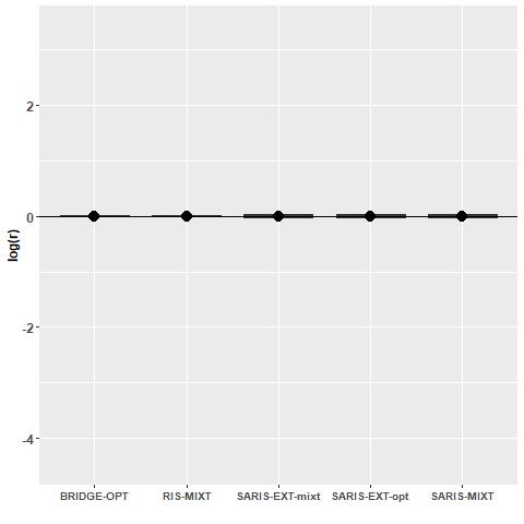
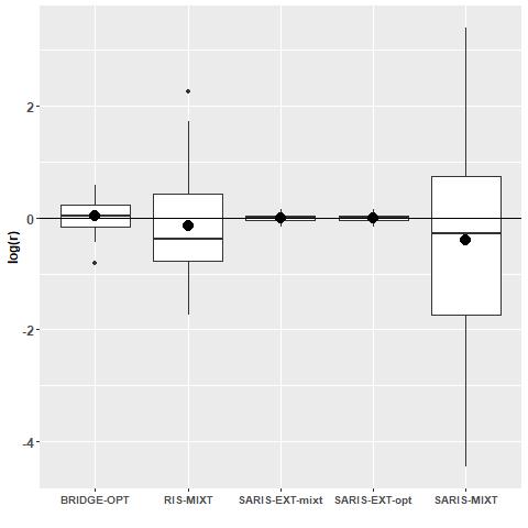
As the theory suggests, the optimal bridge sampling estimator outperforms the two other methods based on samples from and . However, when considering the case , the five methods present performances of the same order. The fact that the bridge like ratio importance sampling performs better than the SARIS-MIXT estimator can be interpreted by the fact that the ratio importance sampling estimator imposes at each step the estimator to solve the empirical version of the SARIS identity (11), which might enhance the stability of the procedure. This difference should be diminished by considering adaptive step sizes, to mimic the differences between and .
Figure 1 illustrates the fact that the SARIS-EXT estimators presented are much more robust to little overlap than ratio importance sampling and Bridge sampling. However, it also illustrates the fact that in more simple cases such as the one illustrated in Figure 1, methods that only use draws from and , which are easier to apply might be sufficient.
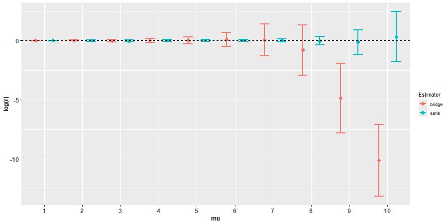
To show intermediate results between the cases and , and worse ones, we compare the optimal Bridge sampling estimator with the SARIS-EXT-opt estimator for varying values of between and . For the simulations we use samples for each expectation in the bridge sampling estimation procedure, and therefore use samples for the SARIS procedure. Results are displayed in Figure 2. For each value of , 50 repetitions were computed. The dots represent the empirical means and the errorbars the empirical standard deviations computed over the 50 repetitions. Figure 2 illustrates the robustness of the proposed procedure in comparison to the bridge sampling estimator that highly deteriorates when the overlap reduces. This makes the proposed procedure appealing when little information is available on the distributions.
5.2 Joint estimation in latent variables models
To illustrate the joint procedure presented above, we consider the following model of linear regression with missing values. Let , we observe the response modeled as :
| (23) |
where is a sequence of independent and identically distributed Gaussian noise with known variance , is an unknown vector of regression coefficients, and is an independent and identically distributed sample of covariates from a . We suppose that for we only observe and for we observe . This example is borrowed from the lecture notes of Julie Josse ”Handling Missing values” available on this website111https://juliejosse.com/wp-content/uploads/2018/07/LectureMissing_Weij_modifAude.html. Here the parameter to estimate is . In order to make the notations as simple as possible, we will confound the notations of the random variables and their observed realizations. Furthermore, we are going to write the density of the random variable evaluated at . For example is the conditional density of given .
With these notations, the complete likelihood is given by :
However we do not observe the first that are handled as latent variables, therefore the observed likelihood is marginalized over their distribution :
In fact we can compute exactly the marginal likelihood as the conditional distribution of given is a .
Given a realization of the unobserved variables, we introduce the complete log likelihood defined as :
We consider here the following test :
To apply the joint procedure described in Section 4.2 we consider the unconstrained parameter space corresponding to the alternative hypothesis, and the constrained parameter that corresponds to the case . For the two estimation procedures, we used stochastic gradient descent. At each step the procedure computes an estimator of the log likelihood ratio, jointly to the estimators and of respectively the restricted and unrestricted maximum likelihood estimators as follows :
-
1.
Draw from the posterior distribution of given and from the posterior distribution of given
-
2.
Update and each with a gradient step :
-
3.
Draw from a uniform distribution on
-
4.
Update as :
For the following experiments, we used a constant step size of for the SARIS procedure and the estimation processes to keep the speed of convergence of the different iterations as similar as possible. The parameters used to generate the data are , , and . Finally, we considered individuals and two different numbers of missing values. We considered which corresponds to of missing values for the second covariate, and then which corresponds to . We used iterations for the estimation process. We reproduced the experiment 20.
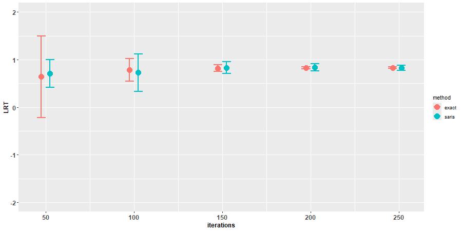
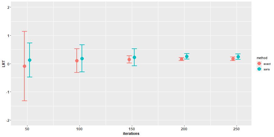
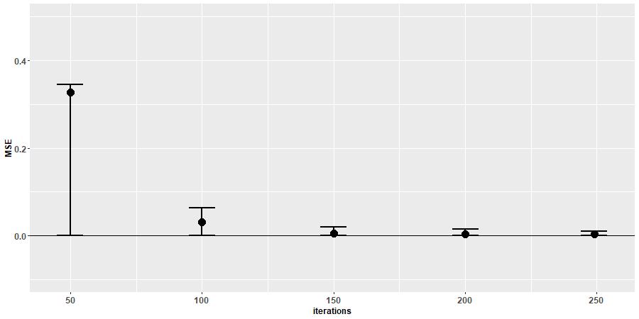
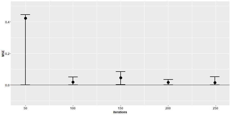
Figure 4 displays the evolution of the exact likelihood ratio over the iterations, compared to the one of the SARIS estimator obtained using the joint procedure described in Section 4.2. The dots represent the mean, and the errorbars the standard deviations computed over the 20 repetitions of the experiment. Figure 4 plots the mean squared error between the exact log likelihood ratio along the iteration process and its approximation using the SARIS joint procedure. The dots are the mean over the 20 repetitions, and the errorbars reach the 5% and 95% corresponding empirical quantiles.
In the case where we observe that the joint procedure accurately tracks the exact value of the likelihood ratio along the estimation process which is very encouraging. We observe that in the more complex case where the joint procedure correctly tracks the exact likelihood ratio statistic but with a small bias. There might be several sources for this bias such as the difference in convergence speed of both estimation processes or the higher variance due to the higher number of missing data. However, the approximation still tracks the exact value along iterations, which makes the proposed joined procedure appealing as a first step of a marginal likelihood computation. Indeed it gives a first estimator at the end of the estimation process that might be used as a starting point for a SARIS procedure, or an estimator to use the approximated optimal scheme of [8] to use as proposal distribution in a ratio importance sampling procedure.
All the experiments were computed on R version 4.3.3 (2024-02-29 ucrt). For reproducibility the scripts are available at this link222https://github.com/tguedon/saris.
6 Conclusion
We proposed a new methodology to compute ratios of normalizing constants that relies on the principle of stochastic approximation. Our procedure presents good theoretical properties which makes it competitive with the best methods from the literature. More precisely, our estimator is consistent and asymptotically Gaussian as the number of iterations goes to infinity. Moreover, the practical implementation of the algorithm reaches an asymptotic variance which is smaller than the optimal variance of the Bridge sampling estimator. Another important advantage is that our estimator does not require to fix in advance the computational effort thanks to its iterative nature. Indeed our procedure can be stopped in practice once a given convergence criterion is reached. Furthermore, our estimator seems more robust to little overlap between the two unnormalised distributions considered and outperforms the Bridge sampling estimator in some of the numerical examples considered. The proposed methodology also allows for the computation of single marginal likelihoods. Moreover, in the context of likelihood ratio test statistics in latent variables models, our procedure can be integrated in the parameter estimation process to reduce the computational effort.
Besides these positive points, there are several interesting perspectives to investigate. Thanks to the rich literature on stochastic approximation and more specifically on stochastic gradient descent, many refinements can be explored, such as acceleration, variance reduction or adaptive step sizes. Similarly, refinements used in classical Monte Carlo such as the Warp Bridge sampling [24, 35] could be applied to reduce the asymptotic variance of the estimator. Furthermore, as a method to compute ratios of normalizing constants, the SARIS procedure can benefit from the use of intermediate distributions that enable to decompose the problem into several simpler sub-problems, in the principle of stepping stone sampling.
7 Declarations
7.1 Funding
This work was funded by the Stat4Plant project ANR-20-CE45-0012.
7.2 Conflict of interest
The authors declare that they have no conflict of interest.
References
- \bibcommenthead
- Annis et al. [2019] Annis, J., Evans, N.J., Miller, B.J., Palmeri, T.J.: Thermodynamic integration and steppingstone sampling methods for estimating bayes factors: A tutorial. Journal of mathematical psychology 89, 67–86 (2019)
- Allassonniere and Kuhn [2015] Allassonniere, S., Kuhn, E.: Convergent stochastic expectation maximization algorithm with efficient sampling in high dimension. application to deformable template model estimation. Computational Statistics & Data Analysis 91, 4–19 (2015)
- Baey et al. [2023] Baey, C., Delattre, M., Kuhn, E., Leger, J.-B., Lemler, S.: Efficient preconditioned stochastic gradient descent for estimation in latent variable models. Proceedings of the 40th International Conference on Machine Learning (2023)
- Bennett [1976] Bennett, C.H.: Efficient estimation of free energy differences from monte carlo data. Journal of Computational Physics 22(2), 245–268 (1976)
- Brekelmans et al. [2020] Brekelmans, R., Masrani, V., Bui, T., Wood, F., Galstyan, A., Steeg, G.V., Nielsen, F.: Annealed importance sampling with q-paths. arXiv preprint arXiv:2012.07823 (2020)
- Benveniste et al. [2012] Benveniste, A., Métivier, M., Priouret, P.: Adaptive Algorithms and Stochastic Approximations vol. 22. Springer, & Business Media (2012)
- Chen and Shao [1997a] Chen, M.-H., Shao, Q.-M.: Estimating ratios of normalizing constants for densities with different dimensions. Statistica Sinica, 607–630 (1997)
- Chen and Shao [1997b] Chen, M.-H., Shao, Q.-M.: On monte carlo methods for estimating ratios of normalizing constants. The Annals of Statistics 25(4), 1563–1594 (1997)
- Delyon et al. [1999] Delyon, B., Lavielle, M., Moulines, E.: Convergence of a stochastic approximation version of the em algorithm. Annals of statistics, 94–128 (1999)
- Del Moral et al. [2006] Del Moral, P., Doucet, A., Jasra, A.: Sequential monte carlo samplers. Journal of the Royal Statistical Society Series B: Statistical Methodology 68(3), 411–436 (2006)
- Duflo [1996] Duflo, M.: Algorithmes Stochastiques vol. 23. Springer, (1996)
- Fort [2015] Fort, G.: Central limit theorems for stochastic approximation with controlled markov chain dynamics. ESAIM: Probability and Statistics 19, 60–80 (2015)
- Frühwirth-Schnatter [2004] Frühwirth-Schnatter, S.: Estimating marginal likelihoods for mixture and markov switching models using bridge sampling techniques. The Econometrics Journal 7(1), 143–167 (2004)
- Friel and Wyse [2012] Friel, N., Wyse, J.: Estimating the evidence–a review. Statistica Neerlandica 66(3), 288–308 (2012)
- Fan et al. [2011] Fan, Y., Wu, R., Chen, M.-H., Kuo, L., Lewis, P.O.: Choosing among partition models in bayesian phylogenetics. Molecular biology and evolution 28(1), 523–532 (2011)
- Gelfand and Dey [1994] Gelfand, A.E., Dey, D.K.: Bayesian model choice: asymptotics and exact calculations. Journal of the Royal Statistical Society: Series B (Methodological) 56(3), 501–514 (1994)
- Geyer [1994] Geyer, C.J.: Estimating normalizing constants and reweighting mixtures (1994)
- Gelman and Meng [1998] Gelman, A., Meng, X.-L.: Simulating normalizing constants: From importance sampling to bridge sampling to path sampling. Statistical science, 163–185 (1998)
- Gronau et al. [2017] Gronau, Q.F., Sarafoglou, A., Matzke, D., Ly, A., Boehm, U., Marsman, M., Leslie, D.S., Forster, J.J., Wagenmakers, E.-J., Steingroever, H.: A tutorial on bridge sampling. Journal of mathematical psychology 81, 80–97 (2017)
- Gronau et al. [2020] Gronau, Q.F., Singmann, H., Wagenmakers, E.-J.: bridgesampling: An r package for estimating normalizing constants. Journal of Statistical Software 92(10), 1–29 (2020)
- Kuhn and Lavielle [2004] Kuhn, E., Lavielle, M.: Coupling a stochastic approximation version of em with an mcmc procedure. ESAIM: Probability and Statistics 8, 115–131 (2004)
- Llorente et al. [2023] Llorente, F., Martino, L., Delgado, D., Lopez-Santiago, J.: Marginal likelihood computation for model selection and hypothesis testing: an extensive review. SIAM Review 65(1), 3–58 (2023)
- Lartillot and Philippe [2006] Lartillot, N., Philippe, H.: Computing bayes factors using thermodynamic integration. Systematic biology 55(2), 195–207 (2006)
- Meng and Schilling [2002] Meng, X.-L., Schilling, S.: Warp bridge sampling. Journal of Computational and Graphical Statistics 11(3), 552–586 (2002)
- Meng and Wong [1996] Meng, X.-L., Wong, W.H.: Simulating ratios of normalizing constants via a simple identity: a theoretical exploration. Statistica Sinica, 831–860 (1996)
- Neal [2001] Neal, R.M.: Annealed importance sampling. Statistics and computing 11, 125–139 (2001)
- Newton and Raftery [1994] Newton, M.A., Raftery, A.E.: Approximate bayesian inference with the weighted likelihood bootstrap. Journal of the Royal Statistical Society Series B: Statistical Methodology 56(1), 3–26 (1994)
- Robert and Casella [1999] Robert, C.P., Casella, G.: Monte Carlo Statistical Methods vol. 2. Springer, New York, NY (1999)
- Robbins and Monro [1951] Robbins, H., Monro, S.: A stochastic approximation method. The annals of mathematical statistics, 400–407 (1951)
- Russel et al. [2018] Russel, P.M., Meyer, R., Veitch, J., Christensen, N.: The stepping-stone sampling algorithm for calculating the evidence of gravitational wave models. arXiv preprint arXiv:1810.04488 (2018)
- Roberts and Rosenthal [2009] Roberts, G.O., Rosenthal, J.S.: Examples of adaptive mcmc. Journal of computational and graphical statistics 18(2), 349–367 (2009)
- Shirts and Chodera [2008] Shirts, M.R., Chodera, J.D.: Statistically optimal analysis of samples from multiple equilibrium states. The Journal of chemical physics 129(12) (2008)
- Torrie and Valleau [1977] Torrie, G.M., Valleau, J.P.: Nonphysical sampling distributions in monte carlo free-energy estimation: Umbrella sampling. Journal of Computational Physics 23(2), 187–199 (1977)
- Van der Vaart [2000] Vaart, A.W.: Asymptotic Statistics vol. 3. Cambridge university press, (2000)
- Wang et al. [2022] Wang, L., Jones, D.E., Meng, X.-L.: Warp bridge sampling: The next generation. Journal of the American Statistical Association 117(538), 835–851 (2022)
- Xie et al. [2011] Xie, W., Lewis, P.O., Fan, Y., Kuo, L., Chen, M.-H.: Improving marginal likelihood estimation for bayesian phylogenetic model selection. Systematic biology 60(2), 150–160 (2011)
Appendix A Proofs
A.1 Proof of Proposition 1
We apply the almost sure convergence theorem of Robbins-Monro algorithms [29] stated in section 5.1 of [6] to prove Proposition 1.
Under Assumption 1 we can define the function for every by where stands for for sake of simplicity. It follows directly that for every and . We define the filtration corresponding to the increasing family of -algebra generated by . We now verify the following assumptions of the theorem stated in section 5.1 of [6]:
-
1.
for any positive measurable function defined on we have
-
2.
there exists , such that for every
-
3.
there exists such that for every :
-
4.
and
The first point is straightforward considering the sampling scheme of equation (14).
We now consider point 2):
thanks to Assumption 1.
Point 3) is straightforward as . Finally point 4) is implied by Assumption 3.
A.2 Proof of Proposition 2
We apply the central theorem for Robbins-Monro algorithms ([11] chapter 4) to prove Proposition 2. The additional assumptions to verify are:
-
1.
There exists a neighborhood of such that the function is continuously differentiable on and for all , .
-
2.
There exists , such that almost surely:
-
3.
There exists such that
-
4.
There exist , , such that the sequence of step sizes is of the form .
The first point is straightforward as is linear in and is constant equal to . To prove the second point, let us introduce for all integer . After some calculation, we get:
Under Assumptions 1 and 6, the sequence converges almost surely to , , and, applying the dominated convergence theorem, the following convergence holds almost surely:
The right hand side term is positive under Assumption 4. Finally we show that Assumption 5 implies condition 3) using similar calculation and arguments. Assumption 6 corresponds to condition 4).
Applying the central theorem for Robbins-Monro algorithms ([11] chapter 4) we get that:
We then apply Jensen inequality to get the minorization:
Moreover the equality case holds in Jensen inequality for which leads to the result.
A.3 Proof of Proposition 3
This proof follows the lines of the proof of Proposition 1. The only difference is that the objective function to nullify is :
that verifies for every . The remaining hypothesis are verified thanks to Assumption 7.
Remark 13.
The fact that is strictly positive for all is implied by Assumption 7. would mean that almost surely.
A.4 Proof of Proposition 4
In order to prove this proposition we proceed in two steps. The first step establishes the central limit theorem, the second step shows that the use of the unnormalized density enables to reach the optimal asymptotic variance .
The first step follows the same lines as the proof of Proposition 2, replacing Assumptions 2 and 5 by Assumptions 7 and 8. Assumption 9 ensures the differentiability of in a neighborhood of , and the fact that . Furthermore, . The continuity of and for every are guaranteed by Assumption 1 and the differentiability of . The central limit theorem of [11] chapter 4 concludes this step, and :
Let , and . The second step proves that verifies Assumptions 7, 8 and 9.
First for every and , the quantity is bounded since its absolute value equals 1, and therefore Assumptions 7 and 8 are verified. The main point to verify is Assumption 9. This is not straightforward because of the absolute value in the definition of the function. Let , and . We get
using Assumption 10, and that for , .
To study the differentiability of , we consider and :
Let study the first term.
is almost surely upper-bounded as it is a (unnormalized) density, let its upperbound.
and with Assumption 10. The same calculations hold with and we get that is differentiable on and for every and finally is differentiable on and specifically :
therefore is differentiable on which concludes the proof, as the first part of the proposition shows that .
A.5 Proof of Proposition 5
We first derive the expression of .
We recall the notations: .
We start from the result of Proposition 2:
We then present the main steps to prove the almost sure convergence and the asymptotic normality of the sequence obtained using Algorithm 3. The analysis of this procedure follows the same lines as the one of the SARIS and SARIS-ext procedure. We introduce the notation
and we define under Assumption 1, with , the function
After some calculation, we get
and
which is positive under Assumption 4. Following the same lines as in the proofs of Propositions 1 and 2, it is straightforward to check that all the assumptions required for the consistency and asymptotic normality hold. Applying these results to the sequence generated by Algorithm 3 leads to the following asymptotic variance :
The optimal bridge sampling asymptotic variance is given in equation (4) by and (see for example Chen and Shao [7, Theorem 5.2.]), which concludes the proof.