ABSTRACT

Although fast radio bursts (FRBs) were discovered more than a decade ago, and they have been one of the active fields in astronomy and cosmology, their origins are still unknown. An interesting topic closely related to the origins of FRBs is their classifications. On the other hand, FRBs are actually a promising probe to study cosmology. In the literature, some new classifications of FRBs different from repeaters and non-repeaters were suggested, and some tight empirical relations have been found for them. In particular, Guo and Wei suggested to classify FRBs into the ones associated with old or young populations, which have also some new empirical relations. They also proposed to use one of the empirical relations without dispersion measure (DM) to calibrate FRBs as standard candles for cosmology. This shows the potential of the new classification and the empirical relations for FRBs. Nowadays, more than 50 FRBs have been well localized, and hence their redshifts $z$ are observationally known. Thus, it is time to check the empirical relations with the current localized FRBs. We find that many empirical relations still hold, and in particular the one used to calibrate FRBs as standard candles for cosmology stands firm.

Checking the Empirical Relations with the Current
Localized Fast Radio Bursts

I Introduction

In the past decade, fast radio bursts (FRBs) NAFRBs ; Lorimer:2018rwi ; Keane:2018jqo ; Petroff:2021wug ; Xiao:2021omr ; Zhang:2020qgp ; Zhang:2022uzl ; Nicastro:2021cxs have been an active field in astronomy and cosmology. One of the key measured quantities of FRBs is the dispersion measure (DM), which is usually large and well in excess of the Galactic values. Since almost all of FRBs are at extragalactic/cosmological distances, they are actually a promising probe to study cosmology and the intergalactic medium (IGM). As a very crude rule of thumb, the redshift of FRB $z\sim{\rm DM}/(1000\;{\rm pc\hskip 2.40005ptcm^{-3}})$ Lorimer:2018rwi . Note that the current observed FRBs reach up to $\rm DM\gtrsim 3000\;{\rm pc\hskip 2.40005ptcm^{-3}}$ (see e.g. tns ; Spanakis-Misirlis:2022 ; frbstats ; Xu:2023did ; blinkverse ), and hence the inferred redshifts could be $z\sim 3$. Actually, it is expected that FRBs are detectable up to redshift $z\sim 15$ in e.g. Zhang:2018csb . So, FRBs could be a useful probe for cosmology, complementary to e.g. type Ia supernovae (SNIa) and cosmic microwave background (CMB).

Although FRBs have been discovered more than a decade ago, their origins are still unknown NAFRBs ; Lorimer:2018rwi ; Keane:2018jqo ; Petroff:2021wug ; Xiao:2021omr ; Zhang:2020qgp ; Zhang:2022uzl ; Nicastro:2021cxs . To this end, a lot of theoretical models were proposed in the literature (see e.g. the living FRB theory catalog Platts:2018hiy ; frbtheorycat ). On the other hand, the observational data were rapidly accumulated in the recent years, which are helpful to study e.g. the engine, radiation mechanism, distribution, classification, propagation effect, and cosmological application of FRBs.

An interesting topic closely related to the origins of FRBs is their classifications Caleb:2018ygr . It is natural to ask “ how many different populations of FRBs exsist? ” Actually, it was strongly argued in e.g. Palaniswamy:2017aze ; Zhong:2022uvu that a single population cannot account for the observational data of FRBs. Obviously, different physical mechanisms for the origins of FRBs are required by different classes of FRBs. In the literature Petroff:2021wug ; Xiao:2021omr ; Zhang:2020qgp ; Zhang:2022uzl ; Nicastro:2021cxs ; Caleb:2018ygr , the well-known classification is repeating and non-repeating FRBs. Note that the repeaters rule out the cataclysmic origins for these sources. However, the question is whether the (apparent) non-repeaters are genuinely one-off or not, and it is still extensively debated in the literature.

On the other hand, some new classifications of FRBs different from repeaters and non-repeaters have also been suggested in the literature. For example, similar to the well-known classification of Gamma-ray bursts (GRBs), it was proposed in Li:2021yds to classify FRBs into short ($W<100\,\rm ms$) and long ($W>100\,\rm ms$) bursts, where $W$ is the pulse width. A tight power-law correlation between fluence and peak flux density was found for them. In Xiao:2021viy , the repeating FRBs were classified into classical ($T_{B}\geq 10^{33}\,\rm K$) and atypical ($T_{B}<10^{33}\,\rm K$) bursts, where $T_{B}$ is the brightness temperature. A tight power-law correlation between pulse width and fluence was also found for classical bursts. In Chaikova:2022vnh , two major classes of FRBs featuring different waveform morphologies and simultaneously different distributions of brightness temperature were identified. In the literature, the relevant works based on machine learning are notable.

In Guo:2022wpf , Guo and Wei suggested to classify FRBs into the ones associated with old or young populations. One can call them Classes (a) and (b) FRBs as in Guo:2022wpf ; Guo:2023hgb , or alternatively, oFRBs and yFRBs as in the present work (see below, n.b. Table 1). In fact, this new classification of FRBs is similar to the well-known classification of type I GRBs (typically short and associated with old populations) and type II GRBs (typically long and associated with young populations) Zhang:2006mb ; Kumar:2014upa . The Galactic FRB 200428 associated with the young magnetar SGR 1935+2154 Andersen:2020hvz ; Bochenek:2020zxn ; Lin:2020mpw ; Li:2020qak confirmed that some FRBs originate from young magnetars. So, it is reasonable to expect that the yFRB distribution is closely correlated with star-forming activities. To date, many FRBs are well localized to the star-forming galaxies (or even the star-forming regions in their host galaxies). We present these yFRBs associated with young stellar populations in Table 2. On the other hand, the well-known repeating FRB 20200120E in a globular cluster of the nearby galaxy M81 Bhardwaj:2021xaa ; Kirsten:2021llv ; Nimmo:2021yob suggested that some FRBs are associated with old stellar populations instead. Nowadays, some FRBs are well localized to old galaxies with low star formation rate (or even old regions in their host galaxies). We also present these oFRBs associated with old stellar populations in Table 2.

In addition, it was claimed in Zhang:2021kdu that the bursts of the first CHIME/FRB catalog CHIMEFRB:2021srp ; CHIMEFRB:cat1 as a whole do not track the cosmic star formation history (SFH). In Qiang:2021ljr , it was independently confirmed that the FRB distribution tracking SFH can be rejected at high confidence, and a suppressed evolution (delay) with respect to SFH was found. Thus, it cannot be true that all FRBs are associated with young stellar populations. There must be FRB progenitor formation channels associated with old stellar populations. So, the new classification of FRBs mentioned above, namely Classes (a) and (b) FRBs as in Guo:2022wpf ; Guo:2023hgb (or alternatively, oFRBs and yFRBs as in the present work), has been well motivated.

If the existing classification non-repeaters/repeaters is valid (namely there are genuinely one-off FRBs), one might combine these two classifications to form a new subclassification of FRBs. We present a brief summary of the universal subclassification scheme of FRBs in Table 1. One can call them Type I, II, a, b, Ia, Ib, IIa, IIb FRBs as in Guo:2022wpf ; Guo:2023hgb , respectively. However, these terms might be hard to remember. Note that the term “ rFRBs ” has been strongly suggested for repeating FRBs in e.g. Zhang:2022uzl ; Nicastro:2021cxs ; Yamasaki:2017hdr ; Ouyed:2019ikb ; Pilia:2020ork . On the other hand, in the field of molecular biology, some subclasses of the well-known RNA (ribonucleic acid) RNA and DNA (deoxyribonucleic acid) DNA are called e.g. mRNA, tRNA, rRNA and tmRNA, miRNA, snRNA, crRNA, sgRNA, as well as eDNA, gDNA, cDNA and dsDNA, ssDNA, cfDNA. Therefore, one can also use the new terms nFRBs, rFRBs, oFRBs, yFRBs, noFRBs, nyFRBs, roFRBs, ryFRBs alternatively, as shown in Table 1, while the suffix “ s ” is just for the plural and it can be removed for the singular. They are friendly and easy to remember in fact.

Notice that even if the existing classification non-repeaters/repeaters is invalid (namely there are no genuinely one-off FRBs, and all FRBs repeat), the new classification oFRBs/yFRBs still holds well by itself. Please keep this in mind carefully.

FRBs	Class (a) : associated with old stellar populations ( oFRBs )	Class (b) :  associated with young stellar populations ( yFRBs )
Type I : Non-repeating ( nFRBs )	Type Ia : Non-repeating FRBs  associated with old stellar populations ( noFRBs )	Type Ib : Non-repeating FRBs  associated with young stellar populations ( nyFRBs )
Type II : Repeating ( rFRBs )	Type IIa : Repeating FRBs  associated with old stellar populations ( roFRBs )	Type IIb : Repeating FRBs  associated with young stellar populations ( ryFRBs )

Table 1: A brief summary of the universal subclassification scheme of FRBs proposed in Guo:2022wpf . One can call them Type I, II, a, b, Ia, Ib, IIa, IIb FRBs as in Guo:2022wpf ; Guo:2023hgb , or alternatively, nFRBs, rFRBs, oFRBs, yFRBs, noFRBs, nyFRBs, roFRBs, ryFRBs as in the present work, respectively. See Sec. I for details.

In Guo:2022wpf , Guo and Wei have found some tight empirical relations for the subclasses of nFRBs in the first CHIME/FRB catalog CHIMEFRB:2021srp ; CHIMEFRB:cat1 . For example, there are some tight empirical relations between spectral luminosity $L_{\nu}$ , isotropic energy $E$ and $\rm DM_{E}$ (extragalactic DM), where

$$L_{\nu}=4\pi d_{L}^{2}S_{\nu}\,,\quad\quad E=4\pi d_{L}^{2}\nu_{c}\,F_{\nu}/(1+z)\,,$$ (1)

$${\rm DM_{E}\equiv DM_{obs}-DM_{MW}-DM_{halo}=DM_{IGM}+DM_{host}}/(1+z)\,,$$ (2)

in which $d_{L}$ is the luminosity distance, $S_{\nu}$ is the flux, $F_{\nu}$ is the the specific fluence, $\nu_{c}$ is the central observing frequency, $\rm DM_{obs}$ is the observed DM, and $\rm DM_{MW}$, $\rm DM_{halo}$, $\rm DM_{IGM}$, $\rm DM_{host}$ are the contributions from the Milky Way (MW), the MW halo, IGM, the host galaxy (including interstellar medium of the host galaxy and the near-source plasma), respectively. In Guo:2022wpf , the tight 2D empirical relations for nyFRBs in the first CHIME/FRB catalog are given by

$$\log E=0.8862\log L_{\nu}+10.0664\,,$$ (3)

$$\log L_{\nu}=2.4707\log{\rm DM_{E}}+27.3976\,,$$ (4)

$$\log E=2.2345\log{\rm DM_{E}}+34.2238\,,$$ (5)

where “ $\log$ ” gives the logarithm to base 10, and $E$, $L_{\nu}$ , $\rm DM_{E}$ are in units of erg, erg/s/Hz, ${\rm pc\hskip 2.40005ptcm^{-3}}$, respectively. There are similar 2D empirical relations for noFRBs and all nFRBs ( = noFRBs + nyFRBs) in the first CHIME/FRB catalog, but with quite different slopes and intercepts. On the other hand, some tight 2D empirical relations are found only for noFRBs in the first CHIME/FRB catalog, namely Guo:2022wpf

$$\log F_{\nu}=0.7709\log S_{\nu}+0.3150\,,$$ (6)

$$\log{\rm DM_{E}}=-0.3987\log S_{\nu}+2.5402\,,$$ (7)

$$\log F_{\nu}=-1.2873\log{\rm DM_{E}}+3.6139\,,$$ (8)

where $F_{\nu}$, $S_{\nu}$, $\rm DM_{E}$ are in units of $\rm Jy\,ms$, Jy, ${\rm pc\hskip 2.40005ptcm^{-3}}$, respectively. It is worth noting that there are no such empirical relations for nyFRBs in the first CHIME/FRB catalog. Finally, some tight 3D empirical relations are also found. We refer to Sec. 4 of Guo:2022wpf for details.

In Guo:2023hgb , the empirical $L_{\nu}-E$ relation for yFRBs akin to Eq. (3), namely

$$\log\frac{E}{\rm erg}=a\log\frac{L_{\nu}}{\rm erg/s/Hz}+b\,,$$ (9)

has been proposed to calibrate yFRBs as standard candles for cosmology, where slope $a$ and intercept $b$ are both dimensionless constants. In this way, one can study cosmology by using the luminosity distances $d_{L}$ of yFRBs directly (rather than DMs), which could be obtained from Eq. (9) if $a\not=1$, noting that $d_{L}$ exists implicitly in both $L_{\nu}$ and $E$ (n.b. Eq. (1)). Actually, as shown in Guo:2023hgb by simulations, this method works well. Noting that DM is not involved in the empirical $L_{\nu}-E$ relation, one can avoid the large uncertainties of $\rm DM_{IGM}$ and $\rm DM_{host}$ in DM which plague the FRB cosmology. This shows the potential of the new classification yFRBs/oFRBs and the empirical relations for them.

However, it is well known that most of FRBs in the first CHIME/FRB catalog CHIMEFRB:2021srp ; CHIMEFRB:cat1 are not localized, and hence their redshifts $z$ and the corresponding luminosity distances $d_{L}$ are unknown actually. In finding the empirical relations mentioned above, the redshifts $z$ of FRBs in Guo:2022wpf were inferred from DMs, and hence they are not real redshifts measured directly. Thus, it is natural to ask “ whether these empirical relations for FRBs are real or not? ”

Several years passed after the first CHIME/FRB catalog CHIMEFRB:2021srp ; CHIMEFRB:cat1 . Nowadays, more than 50 FRBs have been well localized, and hence their redshifts $z$ are observationally known. Therefore, it is time to check the empirical relations with the current localized FRBs.

This paper is organized as followings. In Sec. II, we briefly introduce the sample of current localized FRBs. In Sec. III, we consider the empirical relations for the current localized FRBs. In Sec. IV, the uncertainties are also taken into account. In Sec. V, some brief concluding remarks are given.

FRB	R.A.	Dec.	Redshift	$\rm DM_{obs}$	Width	Fluence	Flux	$\nu_{p}$	$\nu_{c}$	$\Delta\nu$	Rep.	Pop.	Telescope	Ref.
(name)	(deg.)	(deg.)	$z$	( ${\rm pc\hskip 2.40005ptcm^{-3}}$ )	(ms)	(Jy ms)	(Jy)	(MHz)	(MHz)	(MHz)	(0/1)	(0/1/2)
20220207C	310.1995	72.8823	0.04304	$262.38\pm 0.01$	0.5	16.2			1405	187.5	0	1	DSA-110	Law:2023ibd
20220307B	350.8745	72.1924	0.248123	$499.27\pm 0.06$	0.5	3.2			1405	187.5	0	1	DSA-110	Law:2023ibd
20220310F	134.7204	73.4908	0.477958	$462.24\pm 0.005$	1.0	26.2			1405	187.5	0	1	DSA-110	Law:2023ibd
20220319D	32.1779	71.0353	0.011228	$110.98\pm 0.02$	0.3	8.0			1405	187.5	0	1	DSA-110	Law:2023ibd
20220418A	219.1056	70.0959	0.622	$623.25\pm 0.01$	1.0	4.2			1405	187.5	0	1	DSA-110	Law:2023ibd
20220506D	318.0448	72.8273	0.30039	$396.97\pm 0.02$	0.5	13.2			1405	187.5	0	1	DSA-110	Law:2023ibd
20220509G	282.67	70.2438	0.0894	$269.53\pm 0.02$	0.5	5.8			1405	187.5	0	0	DSA-110	Law:2023ibd
20220825A	311.9815	72.5850	0.241397	$651.24\pm 0.06$	1.0	5.8			1405	187.5	0	1	DSA-110	Law:2023ibd
20220914A	282.0568	73.3369	0.1139	$631.28\pm 0.04$	0.5	2.6			1405	187.5	0	1	DSA-110	Law:2023ibd
20220920A	240.2571	70.9188	0.158239	$314.99\pm 0.01$	0.5	3.9			1405	187.5	0	1	DSA-110	Law:2023ibd
20221012A	280.7987	70.5242	0.284669	$441.08\pm 0.7$	2.0	5.1			1405	187.5	0	0	DSA-110	Law:2023ibd
20220912A	347.2704	48.7071	0.0771	$219.46\pm 0.042$	4.7	$0.552\pm 0.007$	$0.1174\pm 0.0014$	1479.5	1250	500	1	1	FAST	DeepSynopticArrayTeam:2022rbq ; Zhang:2023eui
20210117A	339.9792	$-16.1515$	0.214	$729.1^{+0.36}_{-0.23}$	$0.14\pm 0.01$	$36^{+28}_{-9}$			1271.5	336	0	2	ASKAP	Bhandari:2022ton
20181220A	348.6982	48.3421	0.02746	$208.66\pm 1.62$	2.95	$3.0\pm 1.7$	$1.33\pm 0.82$	400.2	600	400	0	1	CHIME	Bhardwaj:2023vha ; CHIMEFRB:2021srp ; CHIMEFRB:cat1
20181223C	180.9207	27.5476	0.03024	$111.61\pm 1.62$	1.97	$2.84\pm 0.93$	$1.36\pm 0.51$	479.2	600	400	0	1	CHIME	Bhardwaj:2023vha ; CHIMEFRB:2021srp ; CHIMEFRB:cat1
20190418A	65.8123	16.0738	0.07132	$182.78\pm 1.62$	1.97	$2.2\pm 1.0$	$0.99\pm 0.58$	400.2	600	400	0	1	CHIME	Bhardwaj:2023vha ; CHIMEFRB:2021srp ; CHIMEFRB:cat1
20190425A	255.6625	21.5767	0.03122	$127.78\pm 1.62$	0.98	$31.6\pm 4.2$	$18.6\pm 2.6$	591.8	600	400	0	1	CHIME	Bhardwaj:2023vha ; CHIMEFRB:2021srp ; CHIMEFRB:cat1
20220610A	351.0732	$-33.5137$	1.016	$1458.15^{+0.25}_{-0.55}$	$0.41\pm 0.01$	$45\pm 5$			1271.5	336	0	1	ASKAP	Ryder:2022qpg
20200120E	149.4863	68.8256	$-0.0001$	$87.782\pm 0.003$	$0.16\pm 0.05$	$2.25\pm 0.12$	$1.8\pm 0.9$		600	400	1	0	CHIME	Bhardwaj:2021xaa
20171020A	333.75	$-19.6667$	0.008672	$114.1\pm 0.2$	$3.2\pm 3.2$	$200\pm 500$	117.6		1297	336	0	1	ASKAP	Mahony:2018ddp
20121102A	82.9946	33.1479	0.1927	$557\pm 2$	$3.0\pm 0.5$	1.2	$0.4\pm 0.1$	1600	1375	322.6	1	1	Arecibo	Gordon:2023cgw
20180301A	93.2268	4.6711	0.3304	$536^{+8}_{-13}$	$2.18\pm 0.06$	1.3	$1.2\pm 0.1$	1415	1352	338.281	1	1	Parkes	Gordon:2023cgw ; Price:2019fmc
20180916B	29.5031	65.7168	0.0337	$347.8\pm 0.0058$	3.93	$6.1\pm 1.7$	$1.84\pm 0.72$	603.9	600	400	1	2	CHIME	Gordon:2023cgw ; CHIMEFRB:2021srp ; CHIMEFRB:cat1
20180924B	326.1053	$-40.90$	0.3212	$362.42\pm 0.06$	$1.3\pm 0.09$	$16\pm 1$	12.3		1320	336	0	1	ASKAP	Gordon:2023cgw
20181112A	327.3485	$-52.9709$	0.4755	$589.27\pm 0.03$	$2.1\pm 0.2$	$26\pm 3$			1272.5	336	0	1	ASKAP	Gordon:2023cgw

Table 2: The sample of current 52 localized FRBs. Right Ascension (R.A.) and Declination (Dec.) are given in degree, J2000. $\nu_{p}$, $\nu_{c}$ and $\Delta\nu$ are peak frequency, central frequency and bandwidth, respectively. In the 12th column (Rep.), 0 and 1 indicate non-repeaters and repeaters, respectively. In the 13th column (Pop.), 0, 1 and 2 indicate FRBs associated with old, young and unknown/transitional stellar populations, respectively. See the text for details.

FRB	R.A.	Dec.	Redshift	$\rm DM_{obs}$	Width	Fluence	Flux	$\nu_{p}$	$\nu_{c}$	$\Delta\nu$	Rep.	Pop.	Telescope	Ref.
(name)	(deg.)	(deg.)	$z$	( ${\rm pc\hskip 2.40005ptcm^{-3}}$ )	(ms)	(Jy ms)	(Jy)	(MHz)	(MHz)	(MHz)	(0/1)	(0/1/2)
20190102C	322.4157	$-79.4757$	0.2912	$363.6\pm 0.3$	$1.7\pm 0.1$	$14\pm 1$			1320	336	0	1	ASKAP	Gordon:2023cgw
20190520B	240.5178	$-11.2881$	0.2414	$1201\pm 10$	$8.7\pm 0.8$	$0.075\pm 0.003$			1375	400	1	1	FAST	Gordon:2023cgw
20190608B	334.0199	$-7.8983$	0.1178	$338.7\pm 0.5$	$6.0\pm 0.8$	$26\pm 4$	4.3	1295	1320	336	0	1	ASKAP	Gordon:2023cgw ; Hiramatsu:2022tyn
20190611B	320.7456	$-79.3976$	0.3778	$321.4\pm 0.2$	$2\pm 1$	$10\pm 2$		1152	1320	336	0	1	ASKAP	Gordon:2023cgw
20190711A	329.4193	$-80.358$	0.522	$593.1\pm 0.4$	$6.5\pm 0.5$	$34\pm 3$		1152	1320	336	1	1	ASKAP	Gordon:2023cgw ; Macquart:2020lln
20190714A	183.9797	$-13.021$	0.2365	$504.13\pm 2.0$	1	8	8	1272.5	1272.5	336	0	1	ASKAP	Gordon:2023cgw ; Hiramatsu:2022tyn ; HESS:2021smp ; Guidorzi:2020ggq
20191001A	323.3513	$-54.7478$	0.234	$506.92\pm 0.04$	$0.22\pm 0.03$	$143\pm 15$		1088	920.5	336	0	1	ASKAP	Gordon:2023cgw ; Bhandari:2020cde
20200430A	229.7064	12.3768	0.1608	$380.1\pm 0.4$		$35\pm 4$		864.5	864.5	336	0	1	ASKAP	Gordon:2023cgw ; Hiramatsu:2022tyn
20200906A	53.4962	$-14.0832$	0.3688	$577.8\pm 0.2$	$6.0\pm 0.2$	$59^{+25}_{-10}$	9.8	864.5	864.5	336	0	1	ASKAP	Gordon:2023cgw ; Hiramatsu:2022tyn
20201124A	77.0146	26.0607	0.0979	$415.3\pm 0.63$	$22\pm 1$	$6\pm 2$	$0.8\pm 0.5$	668	600	400	1	1	CHIME	Gordon:2023cgw ; Lanman:2021yba
20210320C	204.4608	$-16.1227$	0.2797	$384.8\pm 0.3$					864.5	336	0	1	ASKAP	Gordon:2023cgw
20210410D	326.0863	$-79.3182$	0.1415	$571.2\pm 1.0$		35.4	1.5	1711.58	1284	856	0	2	MeerKAT	Gordon:2023cgw ; Caleb:2023atr
20210807D	299.2214	$-0.7624$	0.1293	$251.9\pm 0.2$		$113\pm 9$			920.5	336	0	0	ASKAP	Gordon:2023cgw
20211127I	199.8082	$-18.8378$	0.0469	$234.83\pm 0.08$	1.182	$31\pm 1$		1271.5	1271.5	336	0	1	ASKAP	Gordon:2023cgw
20211203C	204.5625	$-31.3801$	0.3439	$636.2\pm 0.4$		$28\pm 2$			920.5	336	0	1	ASKAP	Gordon:2023cgw
20211212A	157.3509	1.3609	0.0707	$206\pm 5$					1631.5	336	0	1	ASKAP	Gordon:2023cgw
20220105A	208.8039	22.4665	0.2785	$583\pm 1$					1631.5	336	0	1	ASKAP	Gordon:2023cgw
20191106C	199.5801	42.9997	0.10775	$332.2\pm 0.7$	10.81	$1.48\pm 0.26$		618.5	600	400	1	1	CHIME	Ibik:2023ugl ; CHIMEFRB:2021srp ; CHIMEFRB:cat1
20200223B	8.2695	28.8313	0.06024	$201.8\pm 0.4$	3.93	$1.06\pm 0.36$		754.9	600	400	1	1	CHIME	Ibik:2023ugl ; CHIMEFRB:2021srp ; CHIMEFRB:cat1
20190110C	249.3185	41.4434	0.12244	$221.6\pm 1.6$	0.39	$1.4\pm 0.76$	$0.64\pm 0.39$	427.4	600	400	1	1	CHIME	Ibik:2023ugl ; CHIMEFRB:2021srp ; CHIMEFRB:cat1
20190303A	207.9958	48.1211	0.064	$223.2\pm 0.017$	3.93	$2.54\pm 0.97$	$0.47\pm 0.26$	631.5	600	400	1	1	CHIME	Michilli:2022bbs ; CHIMEFRB:2021srp ; CHIMEFRB:cat1
20180814A	65.6833	73.6644	0.068	$190.9\pm 0.076$	7.86	$2.6\pm 1.0$	$0.39\pm 0.3$	464.2	600	400	1	0	CHIME	Michilli:2022bbs ; CHIMEFRB:2021srp ; CHIMEFRB:cat1
20210405I	255.3397	$-49.5451$	0.066	$565.17\pm 0.49$	$8.67\pm 0.28$	120.8	15.9	1016.5	1284	1712	0	0	MeerKAT	Driessen:2023lxj
20191228A	344.4304	$-28.5941$	0.2432	$297.5\pm 0.05$	$2.3\pm 0.6$	$40^{+100}_{-40}$	17	1271.5	1272.5	336	0	1	ASKAP	Bhandari:2021pvj
20181030A	158.5838	73.7514	0.00385	$103.5\pm 0.3$	1.97	$8.2\pm 5.9$	$4.3\pm 3.6$	703.7	600	400	1	1	CHIME	Bhardwaj:2021hgc ; CHIMEFRB:2021srp ; CHIMEFRB:cat1
20190523A	207.065	72.4697	0.66	$760.8\pm 0.6$	$0.42\pm 0.05$	280	660	1530	1411	152.6	0	0	DSA-110	Ravi:2019alc
20190614D	65.0755	73.7067	0.6	$959.2\pm 5.0$	5	$0.62\pm 0.07$	$0.124\pm 0.014$		600	400	0	2	CHIME	Law:2020cnm ; Hiramatsu:2022tyn

Table 2: Continued.

II The sample of current localized FRBs

The sample of current localized FRBs used in this work are mainly compiled from DSA-110, ASKAP, CHIME/FRB and other telescopes. We present them in Table 2, which consists of 52 localized FRBs in total, while the references are also given. Notice that the redshift of FRB 20200120E reads $-0.0001$, which is blueshift in fact, due to its peculiar velocity towards us. It is extremely close to us, so that it is decoupled from the cosmic expansion in fact. On the other hand, the observed $\rm DM_{obs}$ of FRB 20220319D is much less than the $\rm DM_{MW}$ obtained from NE2001 Cordes:2002wz ; Cordes:2003ik ; Ocker:2024rmw ; ne2001p ; Price:2021gzo ; pygedm and YMW16 YMW16 ; Price:2021gzo ; pygedm , namely its $\rm DM_{E}<0$. Although it was shown in Ravi:2023zfl that uncertainties in NE2001 and YMW16 could still accommodate an extragalactic origin for FRB 20220319D, we consider that it is better to be conservative. So, we exclude FRBs 20200120E and 20220319D from Table 2, and 50 localized FRBs are left.

In principle, the fluence $F_{\nu}$ is an integral of flux $S_{\nu}$ with respect to time. If the pulse width $W$ of FRB is small enough ($W\sim{\cal O}(\rm ms)$ or smaller in fact), one has $F_{\nu}\simeq S_{\nu}W$. So, one could approximately estimate $\rm flux\simeq fluence/width$, as in the literature (e.g. Petroff:2016tcr ). In Table 2, the observed values of the fluxes or the widths are absent for some FRBs, and they could be estimated from this approximation. Unfortunately, for six FRBs in Table 2 (20200430A, 20210320C, 20210807D, 20211203C, 20211212A, 20220105A), at least two of width, flux, fluence are absent, and hence the estimation $\rm flux\simeq fluence/width$ cannot work. Thus, we drop them out, and then 44 localized FRBs are left in our sample.

Some derived quantities are required to check the empirical relations. For a given FRB, $\rm DM_{MW}$ can be obtained by using NE2001 Cordes:2002wz ; Cordes:2003ik ; Ocker:2024rmw ; ne2001p ; Price:2021gzo ; pygedm with its Right Ascension (R.A.) and Declination (Dec.) from Table 2. Following e.g. Guo:2022wpf ; Dolag:2014bca ; Prochaska:2019mn , we adopt $\rm DM_{halo}=30\,{\rm pc\hskip 2.40005ptcm^{-3}}$. So, its $\rm DM_{E}=DM_{obs}-DM_{MW}-DM_{halo}$ is on hand. Since the redshift $z$ of a localized FRB is observationally known, its luminosity distance $d_{L}$ is given by

$$d_{L}=\left(1+z\right)d_{C}=\left(1+z\right)\frac{c}{H_{0}}\int_{0}^{z}\frac{d\tilde{z}}{h(\tilde{z})}\,,\quad\quad h(z)=\left[\Omega_{m}\left(1+z\right)^{3}+\left(1-\Omega_{m}\right)\right]^{1/2}\,,$$ (10)

where $d_{C}$ is the comoving distance, $c$ is the speed of light, $H_{0}$ is the Hubble constant, and we adopt $\Omega_{m}=0.3153$, $H_{0}=67.36\,{\rm km/s/Mpc}$ from the Planck 2018 results Aghanim:2018eyx . Thus, the spectral luminosity $L_{\nu}$ and isotropic energy $E$ can be obtained from Eq. (1). On the other hand, the brightness temperature $T_{B}$ is given by (e.g. Guo:2022wpf ; Xiao:2021viy ; Pietka:2014wra ; Majid:2021uli )

$$T_{B}=\frac{S_{\nu}\,d_{L}^{2}}{2\pi\kappa_{B}\left(\nu W\right)^{2}}=1.1\times 10^{35}\,{\rm K}\,\left(\frac{S_{\nu}}{\rm Jy}\right)\left(\frac{d_{L}}{\rm Gpc}\right)^{2}\left(\frac{\nu}{\rm GHz}\right)^{-2}\left(\frac{W}{\rm ms}\right)^{-2}\,,$$ (11)

where $\kappa_{B}$ is the Boltzmann constant. Noting that the peak frequencies $\nu_{p}$ are absent for half of FRBs in Table 2, we use $\nu$ as the central frequency $\nu_{c}$ in Eq. (11).

Since the conclusions of Bhandari:2022ton ; Gordon:2023cgw on the star-forming activity of the host galaxy of FRB 20210117A are fairly different, we assign $\tt Pop.=2$ (namely unknown/transitional) to it in Table 2. On the other hand, actually we have also compiled the spectral indices and other observational quantities for the localized FRBs. However, they are absent for most of FRBs in Table 2, and no significant empirical correlations are found for them. So, we do not include them in Table 2.

III Empirical relations for the current localized FRBs

Since we have only 44 usable localized FRBs as mentioned in Sec. II, it is reasonable to consider the empirical relations just for the (large) classes yFRBs and oFRBs, or nFRBs and rFRBs, rather than the (small) subclasses nyFRBs, noFRBs, ryFRBs, roFRBs.

At first, we linearly fit the data points without error bars (and we will take uncertainties into account in Sec. IV). This can be done by using sklearn.linear_-model.LinearRegression in Python LinearRegression , which employs the ordinary least squares linear regression. The score (coefficient of determination) is given by $R^{2}\equiv 1-\sum_{k}\left(y_{k}-\hat{y}_{k}\right)^{2}/\sum_{k}\left(y_{k}-\bar{y}\right)^{2}$, where $y_{k}$, $\hat{y}_{k}$ and $\bar{y}$ are the observed values, regressed values and mean of observed values LinearRegression ; Xiao:2021viy ; Guo:2022wpf , respectively. The higher $R$ indicates the better fit, and $R=1$ at best. For simplicity, we only consider 2D empirical relations in this work.

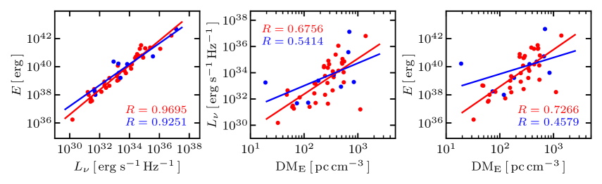
Figure 1: The empirical relations (red/blue lines) between spectral luminosity $L_{\nu}$, isotropic energy $E$ and $\rm DM_{E}$ for 35 localized yFRBs (red points) and 9 localized oFRBs (blue points), respectively. The corresponding $R$ values (in red/blue) are also given. See Sec. III.1 for details.

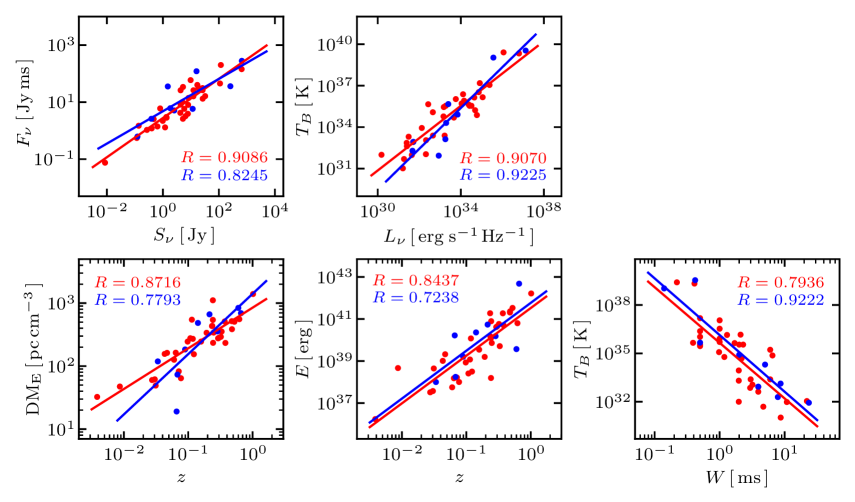
Figure 2: The other five empirical relations (red/blue lines) with high score $R^{2}>0.7$ for 35 localized yFRBs (red points) and 9 localized oFRBs (blue points), respectively. The corresponding $R$ values (in red/blue) are also given. See Sec. III.1 for details.

III.1 Empirical relations for the localized yFRBs and oFRBs

In Guo:2022wpf , some tight empirical relations for nyFRBs and noFRBs in the first CHIME/FRB catalog CHIMEFRB:2021srp ; CHIMEFRB:cat1 have been found, as mentioned in Sec. I. Here, we consider the empirical relations for 35 localized yFRBs (labeled with $\tt Pop.=1$) and 9 localized oFRBs (5 labeled with $\tt Pop.=0$, and 4 labeled with $\tt Pop.=2$, namely we also take FRBs associated with unknown/transitional stellar populations into account, since the number of oFRBs is too few) in Table 2.

In Fig. 1, we check the 2D empirical relations between spectral luminosity $L_{\nu}$ , isotropic energy $E$ and $\rm DM_{E}$ (extragalactic DM) mentioned in Sec. I. As shown by the red lines in Fig. 1, we find that these empirical relations still hold for 35 localized yFRBs, namely

$$\log E=0.8770\log L_{\nu}+10.2853\,,\quad{\rm with}\quad R=0.9695\,,$$ (12)

$$\log L_{\nu}=2.7051\log{\rm DM_{E}}+26.9649\,,\quad{\rm with}\quad R=0.6756\,,$$ (13)

$$\log E=2.6319\log{\rm DM_{E}}+33.3207\,,\quad{\rm with}\quad R=0.7266\,,$$ (14)

with slopes and intercepts close to the ones in Eqs. (3) – (5). The empirical relation (12) is tight, while its $R$ value is higher than the one in Eq. (4.8) of Guo:2022wpf . The $R$ values for empirical relations (13) and (14) are lower than the ones in Eqs. (4.9) and (4.10) of Guo:2022wpf . As shown by the blue lines in Fig. 1, we also find similar empirical relations for 9 localized oFRBs, namely

$$\log E=0.7451\log L_{\nu}+14.8423\,,\quad{\rm with}\quad R=0.9251\,,$$ (15)

$$\log L_{\nu}=1.7177\log{\rm DM_{E}}+29.5783\,,\quad{\rm with}\quad R=0.5414\,,$$ (16)

$$\log E=1.1701\log{\rm DM_{E}}+37.1404\,,\quad{\rm with}\quad R=0.4579\,,$$ (17)

but with quite different slopes and intercepts. The empirical relations (16) and (17) with low $R$ values are somewhat weak, mainly due to the number of localized oFRBs is too few.

In addition, it is of interest to find other empirical relations for the current localized FRBs. We have tried many combinations of the observational and derived quantities. In Fig. 2, we present the other five empirical correlations with high score $R^{2}>0.7$ for both yFRBs and oFRBs. As shown by the red lines in Fig. 2, we find the following empirical relations for 35 localized yFRBs,

$$\log F_{\nu}=0.6875\log S_{\nu}+0.4410\,,\quad{\rm with}\quad R=0.9086\,,$$ (18)

$$\log T_{B}=1.1697\log L_{\nu}-4.2276\,,\quad{\rm with}\quad R=0.9070\,,$$ (19)

$$\log{\rm DM_{E}}=0.6459\log z+2.9285\,,\quad{\rm with}\quad R=0.8716\,,$$ (20)

$$\log E=2.2648\log z+41.5195\,,\quad{\rm with}\quad R=0.8437\,,$$ (21)

$$\log T_{B}=-3.4503\log W+35.6550\,,\quad{\rm with}\quad R=0.7936\,.$$ (22)

There are similar empirical relations for 9 localized oFRBs as shown by the blue lines in Fig. 2, but with quite different slopes and intercepts, namely

$$\log F_{\nu}=0.5673\log S_{\nu}+0.6790\,,\quad{\rm with}\quad R=0.8245\,,$$ (23)

$$\log T_{B}=1.4759\log L_{\nu}-14.7987\,,\quad{\rm with}\quad R=0.9225\,,$$ (24)

$$\log{\rm DM_{E}}=0.9582\log z+3.1489\,,\quad{\rm with}\quad R=0.7793\,,$$ (25)

$$\log E=2.2743\log z+41.7648\,,\quad{\rm with}\quad R=0.7238\,,$$ (26)

$$\log T_{B}=-3.5158\log W+36.1373\,,\quad{\rm with}\quad R=0.9222\,.$$ (27)

The empirical relation (22) for 35 localized yFRBs, and the empirical relations (25) – (26) for 9 localized oFRBs, are somewhat weak as shown by their relatively low $R$ values.

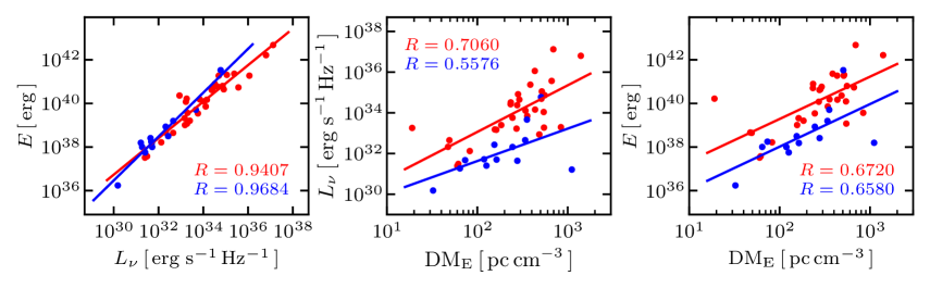
Figure 3: The empirical relations (red/blue lines) between spectral luminosity $L_{\nu}$, isotropic energy $E$ and $\rm DM_{E}$ for 31 localized nFRBs (red points) and 13 localized rFRBs (blue points), respectively. The corresponding $R$ values (in red/blue) are also given. See Sec. III.2 for details.

III.2 Empirical relations for the localized nFRBs and rFRBs

Next, we also consider the empirical relations for 31 localized nFRBs (labeled with $\tt Rep.=0$) and 13 localized rFRBs (labeled with $\tt Rep.=1$) in Table 2.

In Fig. 3, we check the 2D empirical relations between spectral luminosity $L_{\nu}$ , isotropic energy $E$ and $\rm DM_{E}$ (extragalactic DM) mentioned in Sec. I. As shown by the red lines in Fig. 3, we find that these empirical relations still hold for 31 localized nFRBs, namely

$$\log E=0.8373\log L_{\nu}+11.6135\,,\quad{\rm with}\quad R=0.9407\,,$$ (28)

$$\log L_{\nu}=2.2904\log{\rm DM_{E}}+28.4798\,,\quad{\rm with}\quad R=0.7060\,,$$ (29)

$$\log E=1.9405\log{\rm DM_{E}}+35.4052\,,\quad{\rm with}\quad R=0.6720\,,$$ (30)

with slopes and intercepts close to the ones in Eqs. (3) – (5). There are similar empirical relations for 13 localized rFRBs as shown by the blue lines in Fig. 3, namely

$$\log E=1.0066\log L_{\nu}+6.2684\,,\quad{\rm with}\quad R=0.9684\,,$$ (31)

$$\log L_{\nu}=1.5926\log{\rm DM_{E}}+28.4448\,,\quad{\rm with}\quad R=0.5576\,,$$ (32)

$$\log E=1.9537\log{\rm DM_{E}}+34.1080\,,\quad{\rm with}\quad R=0.6580\,,$$ (33)

but with quite different slopes and intercepts. The empirical $L_{\nu}-E$ relation for both nFRBs and rFRBs are tight, as shown by the high $R$ values. But the empirical ${\rm DM_{E}}-L_{\nu}$ and ${\rm DM_{E}}-E$ relations for both nFRBs and rFRBs are somewhat weak, as shown by the relatively low $R$ values.

Again, we try to find more empirical relations for the current localized nFRBs and rFRBs. In Fig. 4, we present the other five empirical correlations with high score $R^{2}>0.7$ for both nFRBs and rFRBs. As shown by the red lines in Fig. 4, we find the following empirical relations for 31 localized nFRBs,

$$\log T_{B}=1.2536\log L_{\nu}-7.0191\,,\quad{\rm with}\quad R=0.8908\,,$$ (34)

$$\log E=2.0861\log z+41.7115\,,\quad{\rm with}\quad R=0.8281\,,$$ (35)

$$\log F_{\nu}=0.6328\log S_{\nu}+0.5049\,,\quad{\rm with}\quad R=0.8040\,,$$ (36)

$$\log L_{\nu}=4.5683\,z+32.7988\,,\quad{\rm with}\quad R=0.7650\,,$$ (37)

$$\log E=4.0127\,z+39.0268\,,\quad{\rm with}\quad R=0.7549\,.$$ (38)

Note that the empirical relations (35) and (38) are different in fact. There are similar empirical relations for 13 localized rFRBs as shown by the blue lines in Fig. 4, namely

$$\log T_{B}=0.8757\log L_{\nu}+4.8644\,,\quad{\rm with}\quad R=0.7433\,,$$ (39)

$$\log E=1.9866\log z+40.6032\,,\quad{\rm with}\quad R=0.8636\,,$$ (40)

$$\log F_{\nu}=0.8093\log S_{\nu}+0.5650\,,\quad{\rm with}\quad R=0.9186\,,$$ (41)

$$\log L_{\nu}=6.9769\,z+31.0184\,,\quad{\rm with}\quad R=0.8593\,,$$ (42)

$$\log E=7.5096\,z+37.4202\,,\quad{\rm with}\quad R=0.8898\,,$$ (43)

but with quite different slopes and intercepts. Please be aware of the difference between the empirical relations (40) and (43).

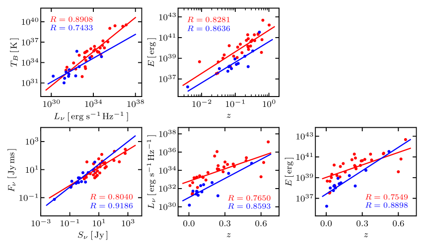
Figure 4: The other five empirical relations (red/blue lines) with high score $R^{2}>0.7$ for 31 localized nFRBs (red points) and 13 localized rFRBs (blue points), respectively. The corresponding $R$ values (in red/blue) are also given. See Sec. III.2 for details.

III.3 Empirical relations for all localized FRBs

It is worth noting that the empirical $L_{\nu}-E$ relation holds solidly in all the cases of yFRBs, oFRBs, nFRBs, rFRBs considered in Secs. III.1 and III.2. Actually, it is tight with high $R$ values close to 1, as shown in Eqs. (12), (15), (28) and (31). Noting that the empirical $L_{\nu}-E$ relation is the key to calibrate FRBs as standard candles for cosmology, as mentioned in Sec. I (see Guo:2023hgb for details), it is of interest to check the empirical relations between spectral luminosity $L_{\nu}$ , isotropic energy $E$ and $\rm DM_{E}$ for all of the current 44 localized FRBs. We present the results in Fig. 5, and they are given by

$$\log E=0.8496\log L_{\nu}+11.2279\,,\quad{\rm with}\quad R=0.9591\,,$$ (44)

$$\log L_{\nu}=2.3922\log{\rm DM_{E}}+27.7618\,,\quad{\rm with}\quad R=0.6345\,,$$ (45)

$$\log E=2.1687\log{\rm DM_{E}}+34.4905\,,\quad{\rm with}\quad R=0.6494\,,$$ (46)

with slopes and intercepts close to the ones in both the cases of yFRBs (n.b. Eqs. (12) – (14)) and nFRBs (n.b. Eqs. (28) – (30)). Although the empirical ${\rm DM_{E}}-L_{\nu}$ and ${\rm DM_{E}}-E$ relations are somewhat weak with low $R$ values, the empirical $L_{\nu}-E$ relation stands firm with high $R$ value close to 1.

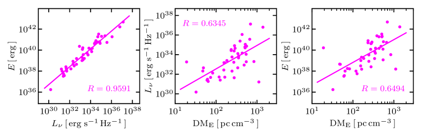
Figure 5: The empirical relations (magenta lines) between spectral luminosity $L_{\nu}$, isotropic energy $E$ and $\rm DM_{E}$ for all 44 localized FRBs (magenta points). The corresponding $R$ values are also given. See Sec. III.3 for details.

IV Taking uncertainties into account

In the previous section, the linear empirical relations are fitted to the data points without error bars by using sklearn.linear_-model.LinearRegression in Python LinearRegression , which employs the ordinary least squares linear regression. In this section, we further take uncertainties into account.

Here, we do not try to consider all empirical relations with uncertainties. We mainly focus on the the empirical relations between spectral luminosity $L_{\nu}$ , isotropic energy $E$ and $\rm DM_{E}$, which are the main empirical relations found in Guo:2022wpf and the key to calibrate FRBs as standard candles for cosmology Guo:2023hgb . But we note that the method used here is very general and can be easily apply to all empirical relations with uncertainties.

It is worth noting that $L_{\nu}$ , $E$ and $\rm DM_{E}$ are all derived quantities. When one takes their uncertainties into account, the error propagation should be considered carefully (see e.g. Alam:2004ip ; Wei:2006va ; Liu:2014vda ; Yin:2018mvu ; Qiang:2020vta ; errorp ). Alternatively, one could use the Python package uncertainties uncertainties to this end. The observed quantities fluence $F_{\nu}$, flux $S_{\nu}$ and $\rm DM_{obs}$ are involved in $L_{\nu}$ , $E$ and $\rm DM_{E}$ (n.b. Eqs. (1) and (2)), while the uncertainties of redshifts $z$ and then $d_{L}$ are negligible. Note that the uncertainties of $F_{\nu}$, $S_{\nu}$ and $\rm DM_{obs}$ are given in Table 2. To be conservative, if the upper and lower errors are not equal, we adopt the larger one. On the other hand, if the errors of some observed quantities are absent in Table 2, we assign the average relative errors in the same columns to them. Noting that the fluxes are absent for some FRBs in Table 2 and they can be estimated by using $\rm flux\simeq fluence/width$ as mentioned in Sec. II, the error propagation should also be considered here. Finally, we obtain the uncertainties of $\log L_{\nu}$ , $\log E$ and $\log{\rm DM_{E}}$ for all of the current 44 localized FRBs, as shown by the horizontal and vertical error bars in Fig. 6. Note that the horizontal error bars of $\log{\rm DM_{E}}$ are too short to be seen by eyes, mainly due to the uncertainties of $\rm DM_{obs}$ for all FRBs are very small, as shown in Table 2.

Next, the linear empirical relations will be fitted to these data points with both the horizontal and vertical error bars. To our best knowledge, there are two main methods to this end in the literature. One might use the bisector of the two ordinary least squares Isobe:1990up (see also e.g. Schaefer:2006pa ; Liang:2008kx ; Wei:2008kq ; Wei:2010wu ; Liu:2014vda ). Alternatively, in this work we use the Nukers’ estimate Tremaine:2002js (see also e.g. Tsvetkova:2017lea ; Minaev:2019unh ). If one fits the linear empirical relation with constant slope $a$ and intercept $b$, namely

$$y=ax+b\,,$$ (47)

to $N$ data points $(x_{i},\ y_{i})$ with errors $\sigma_{xi}$ and $\sigma_{yi}$, the Nukers’ estimate is based on minimizing

$$\chi^{2}=\sum_{i\,=\,1}^{N}\,\frac{(y_{i}-ax_{i}-b)^{2}}{a^{2}\sigma_{xi}^{2}+\sigma_{yi}^{2}+\sigma_{\rm int}^{2}}\,,$$ (48)

where $\sigma_{\rm int}$ represents the intrinsic dispersion, which is determined by requiring $\chi^{2}/dof=1$ Tremaine:2002js (see also e.g. Tsvetkova:2017lea ; Minaev:2019unh ). We minimize $\chi^{2}$ by using the Markov Chain Monte Carlo (MCMC) Python package emcee Foreman-Mackey:2012any with GetDist Lewis:2019xzd and then obtain the constraints on the free parameters $a$ and $b$.

By using this method, we fit the linear empirical relations between $\log L_{\nu}$ , $\log E$ and $\log{\rm DM_{E}}$ to the 44 data points of all localized FRBs with both the horizontal and vertical error bars as shown in Fig. 6. The results are given by

$$\log E=a\log L_{\nu}+b\quad{\rm with}\quad a=0.8336\pm 0.0375,\ b=11.7858\pm 1.2568,\ \sigma_{\rm int}=0.3308\,,$$ (49)

$$\log L_{\nu}=a\log{\rm DM_{E}}+b\quad{\rm with}\quad a=2.3741\pm 0.4527,\ b=27.8054\pm 1.0893,\ \sigma_{\rm int}=1.2292\,,\hskip 28.45274pt$$ (50)

$$\log E=a\log{\rm DM_{E}}+b\quad{\rm with}\quad a=2.1807\pm 0.3967,\ b=34.4443\pm 0.9568,\ \sigma_{\rm int}=1.0591\,,$$ (51)

where the constraints on $a$ and $b$ are given by their medians with $1\sigma$ uncertainties. These linear empirical relations with their median $a$ and $b$ are also plotted in Fig. 6. On the other hand, in Fig. 7, we present the $1\sigma$, $2\sigma$ and $3\sigma$ contours for $a$ and $b$ of these linear empirical relations. From Eqs. (49) – (51) and Fig. 7, it is easy to see that the constraints on $a$ and $b$ are fairly tight. Notice that for the empirical $\log L_{\nu}-\log E$ relation, $a=1$ is certainly far beyond $3\sigma$ region, and it is actually on the edge of $4\sigma$ region. This is fairly good for using the empirical $\log L_{\nu}-\log E$ relation with $a\not=1$ to calibrate FRBs as standard candles for cosmology, as mentioned in Sec. I (see Guo:2023hgb for details).

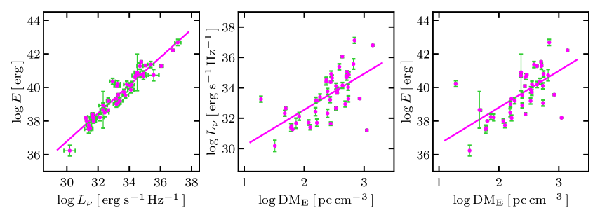
Figure 6: The linear empirical relations (magenta lines) between $\log L_{\nu}$ , $\log E$ and $\log{\rm DM_{E}}$ for all of the 44 localized FRBs (magenta points) with both the horizontal and vertical error bars (in lime green). See Sec. IV for details.

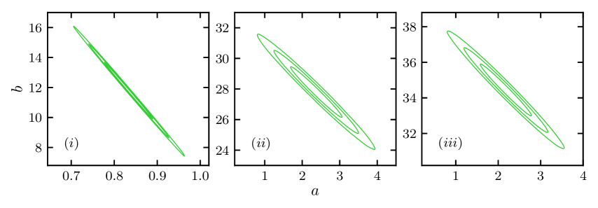
Figure 7: The $1\sigma$, $2\sigma$ and $3\sigma$ contours for slopes $a$ and intercepts $b$ of the linear empirical relations $(i)$ $\log L_{\nu}-\log E$, $(ii)$ $\log{\rm DM_{E}}-\log L_{\nu}$ and $(iii)$ $\log{\rm DM_{E}-\log E}$. See Sec. IV for details.

V Concluding remarks

Although FRBs were discovered more than a decade ago, and they have become one of the active fields in astronomy and cosmology, their origins are still unknown. An interesting topic closely related to the origins of FRBs is their classifications. On the other hand, FRBs are actually a promising probe to study cosmology. In the literature, some new classifications of FRBs different from repeaters and non-repeaters were suggested, and some tight empirical relations have been found for them. In particular, Guo and Wei suggested to classify FRBs into the ones associated with old or young populations, which have also some new empirical relations. They also proposed to use one of the empirical relations without DM to calibrate FRBs as standard candles for cosmology. This shows the potential of the new classification and the empirical relations for FRBs. Nowadays, more than 50 FRBs have been well localized, and hence their redshifts $z$ are observationally known. Thus, it is time to check the empirical relations with the current localized FRBs. We find that many empirical relations still hold, and in particular the one used to calibrate FRBs as standard candles for cosmology stands firm.

Some remarks are in order. Actually, the number of current $44\sim 52$ localized FRBs is not enough. There is still room to doubt. If the number of localized FRBs could be doubled or more than ${\cal O}(10^{2})$ in the near future, and if a large uniform sample of localized FRBs from a single telescope/array is available at that time, we might eliminate the possibility that the selection effects lead to the artificial empirical relations. Let us keep an open mind and wait.

If these empirical relations are real, they are meaningful on two sides. At first, they might support the other classifications of FRBs different from repeaters and non-repeaters, especially the new classification yFRBs/oFRBs proposed in Guo:2022wpf . On the other hand, they might help FRBs to be a promising probe for cosmology. In particular, the empirical $L_{\nu}-E$ relation stands firm with the current localized FRBs, and the slope $a\not=1$ in Eq. (9) far beyond $3\sigma$ confidence level (C.L.), as shown in Sec. IV of this work. If $a=1$, the luminosity distance $d_{L}$ will be canceled in both sides of Eq. (9) (n.b. Eq. (1)), and hence it cannot be used to study cosmology. If $a\not=1$ as shown in this work by using the current localized FRBs, Eq. (9) can be recast as Guo:2023hgb

$$\mu=-\frac{5}{2\left(1-\alpha\right)}\,\log\frac{\;F_{\nu}/(1+z)\,}{\rm Jy\,ms}+\frac{5\alpha}{2\left(1-\alpha\right)}\,\log\frac{S_{\nu}}{\;\rm Jy\,}+\beta\,,$$ (52)

where $\alpha=a\not=1$, $\beta={\rm const.}$ is a complicated combination of $a$ and $b$, while $\mu$ is the well-known distance modulus defined by

$$\mu=5\log\frac{d_{L}}{\,\rm Mpc}+25\,.$$ (53)

As shown in Guo:2023hgb by simulations, Eq. (52) can be used to calibrate the localized FRBs as standard candles for cosmology, complementary to e.g. SNIa, CMB and GRBs.

Finally, different physical mechanisms are required by different classes of FRBs, and different classes of FRBs have different empirical relations. Obviously, the empirical relations of FRBs require some physical mechanisms behind them. Therefore, they might help us to reveal the origins of FRBs. These topics are cross-related, and have important values in this field.

References

- (1) https:www.nature.com/collections/rswtktxcln
- (2) D. R. Lorimer, Nat. Astron. 2, 860 (2018) [arXiv:1811.00195].
- (3) E. F. Keane, Nat. Astron. 2, 865 (2018) [arXiv:1811.00899].
- (4) E. Petroff, J. W. T. Hessels and D. R. Lorimer, Astron. Astrophys. Rev. 30, 2 (2022) [arXiv:2107.10113].
- (5) D. Xiao, F. Y. Wang and Z. G. Dai, Sci. China Phys. Mech. Astron. 64, 249501 (2021) [arXiv:2101.04907].
- (6) B. Zhang, Nature 587, 45 (2020) [arXiv:2011.03500].
- (7) B. Zhang, Rev. Mod. Phys. 95, no.3, 035005 (2023) [arXiv:2212.03972].
- (8) L. Nicastro et al., Universe 7, no.3, 76 (2021) [arXiv:2103.07786].
- (9) TNS, available at https:www.wis-tns.org
- (10) A. Spanakis-Misirlis and C. L. Van Eck, arXiv:2208.03508 [astro-ph.IM].
- (11) FRBSTATS, available at https:www.herta-experiment.org/frbstats
- (12) J. Xu et al., Universe 9, no.7, 330 (2023) [arXiv:2308.00336].
- (13) Blinkverse, available at https:blinkverse.alkaidos.cn
- (14) B. Zhang, Astrophys. J. Lett. 867, no.2, L21 (2018) [arXiv:1808.05277].
- (15) E. Platts et al., Phys. Rept. 821, 1 (2019) [arXiv:1810.05836].
- (16) The living FRB theory catalog, available at https:frbtheorycat.org
- (17) M. Caleb, L. G. Spitler and B. W. Stappers, Nat. Astron. 2, 839 (2018) [arXiv:1811.00360].
- (18) D. Palaniswamy, Y. Li and B. Zhang, Astrophys. J. Lett. 854, no.1, L12 (2018) [arXiv:1703.09232].
- (19) S. Q. Zhong et al., Astrophys. J. 926, no.2, 206 (2022) [arXiv:2202.04422].
- (20) X. J. Li, X. F. Dong, Z. B. Zhang and D. Li, Astrophys. J. 923, no.2, 230 (2021) [arXiv:2110.07227].
- (21) D. Xiao and Z. G. Dai, Astron. Astrophys. 657, L7 (2022) [arXiv:2112.12301].
- (22) A. Chaikova, D. Kostunin and S. B. Popov, arXiv:2202.10076 [astro-ph.HE].
- (23) H. Y. Guo and H. Wei, JCAP 2207, 010 (2022) [arXiv:2203.12551].
- (24) H. Y. Guo and H. Wei, arXiv:2301.08194 [astro-ph.HE].
- (25) B. Zhang et al., Astrophys. J. Lett. 655, L25 (2007) [astro-ph/0612238].
- (26) P. Kumar and B. Zhang, Phys. Rept. 561, 1 (2014) [arXiv:1410.0679].
- (27) B. C. Andersen et al., Nature 587, no. 7832, 54 (2020) [arXiv:2005.10324].
- (28) C. D. Bochenek et al., Nature 587, no. 7832, 59 (2020) [arXiv:2005.10828].
- (29) L. Lin et al., Nature 587, no. 7832, 63 (2020) [arXiv:2005.11479].
- (30) C. K. Li et al., Nat. Astron. 5, 378 (2021) [arXiv:2005.11071].
- (31) M. Bhardwaj et al., Astrophys. J. Lett. 910, no.2, L18 (2021) [arXiv:2103.01295].
- (32) F. Kirsten et al., Nature 602, no.7898, 585 (2022) [arXiv:2105.11445].
- (33) K. Nimmo et al., Nat. Astron. 6, 393 (2022) [arXiv:2105.11446].
- (34) R. C. Zhang and B. Zhang, Astrophys. J. Lett. 924, no.1, L14 (2022) [arXiv:2109.07558].
- (35) M. Amiri et al., Astrophys. J. Supp. 257, no.2, 59 (2021) [arXiv:2106.04352].
- (36) The data for CHIME/FRB Catalog 1 in machine-readable format can be found via their public webpage at https:www.chime-frb.ca/catalog
- (37) D. C. Qiang, S. L. Li and H. Wei, JCAP 2201, 040 (2022) [arXiv:2111.07476].
- (38) S. Yamasaki, T. Totani and K. Kiuchi, Publ. Astron. Soc. Jap. 70, no.3, 39 (2018) [arXiv:1710.02302].
- (39) R. Ouyed, D. Leahy and N. Koning, Res. Astron. Astrophys. 20, no.2, 027 (2020) [arXiv:1906.09559].
- (40) M. Pilia et al., Astrophys. J. Lett. 896, no.2, L40 (2020) [arXiv:2003.12748].
- (41) https:en.wikipedia.org/wiki/RNA
- (42) https:en.wikipedia.org/wiki/DNA
- (43) C. J. Law et al., Astrophys. J. 967, no.1, 29 (2024) [arXiv:2307.03344].
- (44) V. Ravi et al., Astrophys. J. Lett. 949, no.1, L3 (2023) [arXiv:2211.09049].
- (45) Y. K. Zhang et al., Astrophys. J. 955, no.2, 142 (2023) [arXiv:2304.14665].
- (46) S. Bhandari et al., Astrophys. J. 948, no.1, 67 (2023) [arXiv:2211.16790].
- (47) M. Bhardwaj et al., arXiv:2310.10018 [astro-ph.HE].
- (48) S. D. Ryder et al., Science 392, 294 (2023) [arXiv:2210.04680].
- (49) E. K. Mahony et al., Astrophys. J. Lett. 867, no.1, L10 (2018) [arXiv:1810.04354].
- (50) A. C. Gordon et al., Astrophys. J. 954, no.1, 80 (2023) [arXiv:2302.05465].
- (51) D. C. Price et al., Mon. Not. Roy. Astron. Soc. 486, no.3, 3636 (2019) [arXiv:1901.07412].
- (52) D. Hiramatsu et al., Astrophys. J. Lett. 947, no.2, L28 (2023) [arXiv:2211.03974].
- (53) J. P. Macquart et al., Nature 581, no.7809, 391 (2020) [arXiv:2005.13161].
- (54) J. O. Chibueze et al., Mon. Not. Roy. Astron. Soc. 515, no.1, 1365 (2022) [arXiv:2201.00069].
- (55) C. Guidorzi et al., Astron. Astrophys. 637, A69 (2020) [arXiv:2003.10889].
- (56) S. Bhandari et al., Astrophys. J. Lett. 901, no.2, L20 (2020) [arXiv:2008.12488].
- (57) A. E. Lanman et al., Astrophys. J. 927, no.1, 59 (2022) [arXiv:2109.09254].
- (58) M. Caleb et al., Mon. Not. Roy. Astron. Soc. 524, no.2, 2064 (2023) [arXiv:2302.09754].
- (59) A. L. Ibik et al., Astrophys. J. 961, no.1, 99 (2024) [arXiv:2304.02638].
- (60) D. Michilli et al., Astrophys. J. 950, no.2, 134 (2023) [arXiv:2212.11941].
- (61) L. N. Driessen et al., Mon. Not. Roy. Astron. Soc. 527, no.2, 3659 (2023) [arXiv:2302.09787].
- (62) S. Bhandari et al., Astron. J. 163, no.2, 69 (2022) [arXiv:2108.01282].
- (63) M. Bhardwaj et al., Astrophys. J. Lett. 919, no.2, L24 (2021) [arXiv:2108.12122].
- (64) V. Ravi et al., Nature 572, no.7769, 352 (2019) [arXiv:1907.01542].
- (65) C. J. Law et al., Astrophys. J. 899, no.2, 161 (2020) [arXiv:2007.02155].
- (66) J. M. Cordes and T. J. W. Lazio, astro-ph/0207156.
- (67) J. M. Cordes and T. J. W. Lazio, astro-ph/0301598.
- (68) S. K. Ocker and J. M. Cordes, Res. Notes AAS 8, no.1, 17 (2024) [arXiv:2401.05475].
- (69) https:pypi.org/project/mwprop
- (70) D. C. Price, A. Deller and C. Flynn, Publ. Astron. Soc. Austral. 38, e038 (2021) [arXiv:2106.15816].
- (71) https:pypi.org/project/pygedm and https:pygedm.readthedocs.io
- (72) J. M. Yao, R. N. Manchester and N. Wang, Astrophys. J. 835, 29 (2017) [arXiv:1610.09448].
- (73) V. Ravi et al., arXiv:2301.01000 [astro-ph.GA].
- (74) E. Petroff et al., Publ. Astron. Soc. Austral. 33, e045 (2016) [arXiv:1601.03547].
- (75) K. Dolag et al., Mon. Not. Roy. Astron. Soc. 451, no.4, 4277 (2015) [arXiv:1412.4829].
- (76) J. X. Prochaska and Y. Zheng, Mon. Not. Roy. Astron. Soc. 485, no.1, 648 (2019) [arXiv:1901.11051].
- (77) N. Aghanim et al., Astron. Astrophys. 641, A6 (2020) [arXiv:1807.06209].
- (78) M. Pietka, R. P. Fender and E. F. Keane, Mon. Not. Roy. Astron. Soc. 446, 3687 (2015) [arXiv:1411.1067].
- (79) W. A. Majid et al., Astrophys. J. Lett. 919, no.1, L6 (2021) [arXiv:2105.10987].
- (80) https:scikit-learn.org/stable/modules/generated/sklearn.linear-model.LinearRegression.html
- (81) U. Alam, V. Sahni, T. D. Saini and A. A. Starobinsky, astro-ph/0406672.
- (82) H. Wei, N. N. Tang and S. N. Zhang, Phys. Rev. D 75, 043009 (2007) [astro-ph/0612746].
- (83) J. Liu and H. Wei, Gen. Rel. Grav. 47, no.11, 141 (2015) [arXiv:1410.3960].
- (84) Z. Y. Yin and H. Wei, Sci. China Phys. Mech. Astron. 62, no.9, 999811 (2019) [arXiv:1808.00377].
- (85) D. C. Qiang and H. Wei, JCAP 2004, 023 (2020) [arXiv:2002.10189].
- (86) https:en.wikipedia.org/wiki/Propagation-of-uncertainty
- (87) https:pythonhosted.org/uncertainties and https:pypi.org/project/uncertainties
- (88) T. Isobe, E. D. Feigelson, M. G. Akritas and G. J. Babu, Astrophys. J. 364, 104 (1990).
- (89) B. E. Schaefer, Astrophys. J. 660, 16 (2007) [astro-ph/0612285].
- (90) N. Liang, W. K. Xiao, Y. Liu and S. N. Zhang, Astrophys. J. 685, 354 (2008) [arXiv:0802.4262].
- (91) H. Wei and S. N. Zhang, Eur. Phys. J. C 63, 139 (2009) [arXiv:0808.2240].
- (92) H. Wei, JCAP 1008, 020 (2010) [arXiv:1004.4951].
- (93) S. Tremaine et al., Astrophys. J. 574, 740 (2002) [astro-ph/0203468].
- (94) A. Tsvetkova et al., Astrophys. J. 850, no.2, 161 (2017) [arXiv:1710.08746].
- (95) P. Y. Minaev and A. S. Pozanenko, Mon. Not. Roy. Astron. Soc. 492, 1919 (2020) [arXiv:1912.09810].
- (96) D. Foreman-Mackey et al., Publ. Astron. Soc. Pac. 125, 306 (2013) [arXiv:1202.3665].
- (97) A. Lewis, arXiv:1910.13970 [astro-ph.IM].