Confounding Privacy and Inverse Composition

Abstract

We introduce a novel privacy notion of ($\epsilon,\delta$)-confounding privacy that generalizes both differential privacy and Pufferfish privacy. In differential privacy, sensitive information is contained in the dataset while in Pufferfish privacy, sensitive information determines data distribution. Consequently, both assume a chain-rule relationship between the sensitive information and the output of privacy mechanisms. Confounding privacy, in contrast, considers general causal relationships between the dataset and sensitive information. One of the key properties of differential privacy is that it can be easily composed over multiple interactions with the mechanism that maps private data to publicly shared information. In contrast, we show that the quantification of the privacy loss under the composition of independent ($\epsilon,\delta$)-confounding private mechanisms using the optimal composition of differential privacy underestimates true privacy loss. To address this, we characterize an inverse composition framework to tightly implement a target global ($\epsilon_{g},\delta_{g}$)-confounding privacy under composition while keeping individual mechanisms independent and private. In particular, we propose a novel copula-perturbation method which ensures that (1) each individual mechanism $i$ satisfies a target local ($\epsilon_{i},\delta_{i}$)-confounding privacy and (2) the target global ($\epsilon_{g},\delta_{g}$)-confounding privacy is tightly implemented by solving an optimization problem. Finally, we study inverse composition empirically on real datasets.

Keywords First keyword  $\cdot$ Second keyword  $\cdot$ More

1 Introduction

Differential privacy (DP) [1] is a widely adopted statistical framework for protecting individual privacy in data analysis. DP ensures that two datasets differing in a single record produce almost indistinguishable outputs, thereby limiting the information that can be inferred about any individual record. It has become the gold standard for data privacy due to its strong theoretical guarantees and robustness against a wide range of attacks. A key to DP’s success is its ability to quantify and reason about privacy strength and loss under many differentially private interactions (i.e., composition) [2]. However, DP relies on assumptions that may not hold in all scenarios, such as independence of data records, and uniform protection for all attributes. Pufferfish privacy (PP) [3], a framework that generalizes DP, addresses some of these limitations by providing a more flexible approach. PP extends the concept of neighboring datasets in DP to neighboring distributions of datasets [4], captured by discriminative pairs of secrets, which represent sensitive information that requires protection. This allows PP to incorporate domain-specific knowledge and account for data correlations.

However, DP and PP assume the following probabilistic chain-rule relationship between the sensitive information, dataset, and output of a (private) data analysis mechanism:

sensitive information $\rightarrow$ dataset $\rightarrow$ output

In DP, sensitive information impacts the output through the data analysis process. In PP, sensitive information influences the probability distribution of the dataset, which then affects the output. However, as systems become more complex, involving interactions in intricate networked environments, sensitive information may extend beyond individual records or dataset distributions. It may include knowledge that needs to be extracted from the dataset or intermediate information generated by interactions within a large system, possibly through an inner mechanism that cannot be accessed publicly. In such cases, the relationship between sensitive information, the dataset, and the output may be more complex than this chain-rule structure.

In this work, we introduce the notion of confounding privacy (CP) that captures a general causal relationship between the sensitive information and the dataset:

sensitive information $\leftrightharpoons$ dataset $\rightarrow$ output

CP uses a Bayesian approach to establish the relationship between the sensitive information—which we refer to as state—and the output of the mechanism that takes as input the dataset, where the relationship between the state and the dataset is captured probabilistically. The CP framework adopts the $(\epsilon,\delta)$ quantification scheme used by the DP and the PP frameworks to parameterize the probabilistic indistinguishability. We are particularly interested in the ability of CP to quantify the cumulative privacy loss of the state under composition when the same dataset induces the state and is used by multiple independent mechanisms where each mechanism independently satisfies CP.

Our first observation is that CP does not compose as gracefully as DP, an issue it shares with PP. [3] provide a sufficient condition known as universally composable evolution scenarios (UCES) for linear composition. UCES considers a deterministic one-to-one mapping from a secret (along with prior knowledge) to a dataset, allowing PP with UCES to benefit from DP’s composition property by eliminating randomness in the relationship between the secret and the dataset. However, when the relationship between the sensitive information and the dataset does not follow a chain-rule structure, UCES becomes intractable.

In this work, we show that the composition of multiple independent CP mechanisms remains CP. However, we also demonstrate that the optimal composition bound for DP [5, 6] using the $(\epsilon,\delta)$ scheme underestimates the cumulative privacy loss in the CP framework, making it challenging to determine privacy bounds under composition. To address this, we leverage the copula [7] of the joint distribution to separate the correlation component from the independent marginal mechanisms in an additive manner in the privacy loss random variable under composition. A class of privacy loss functions called bound-consistent privacy loss is introduced, which captures the worst-case scenario regardless of specific attack models. We propose inverse composition by leveraging a mechanism-design theoretic approach to implement a target privacy loss bound under composition by solving a convex programming, formulated using any bound-consistent privacy loss and a convex set of conditions. Our inverse composition method avoids the combinatorial explosion of parameters that occurs in the classic composition of DP and does not depend on functional descriptions of the underlying mechanisms used in the find-grained composition of DP. We propose two approaches termed the copula perturbation and the single-shot re-design to perform inverse composition for standard DP mechanisms. Finally, we present experiments on real-world dataset to demonstrate the efficacy of the proposed approach.

1.1 Related Work

The notion of confounding privacy builds upon the definitions of differential privacy [1] and Pufferfish privacy [3] by extending the chain-rule structure from the sensitive information to the dataset to a general probabilistic causation relationship. The primary challenge in implementing PP frameworks lies in the scarcity of suitable mechanisms. Several important instantiations of PP framework have been proposed, including blowfish privacy [8], Wasserstein mechanism [9] for correlated data, attribute privacy [10], and mutual-information PP [11].

1.1.1 Composition of PP

PP does not always compose [3, 9]. [3] provide a sufficient condition known as universally composable evolution scenarios (UCES) for linear self-composition (i.e., similar to the basic composition of DP [1]). UCES considers a deterministic one-to-one mapping from a secret (along with prior knowledge) to a dataset, allowing PP with UCES to benefit from DP’s composition property by eliminating randomness in the relationship between the secret and the dataset. In our CP framework, when the relationship between the state (sensitive information) and the dataset does not follow a chain-rule structure, UCES becomes generally infeasible. This is because causation may flow from the dataset to the state, making it infeasible to pin down a specific dataset for a given state by eliminating randomness in the relationship, particularly when another mechanism controls this relationship for different purposes.

1.1.2 Classic Composition of DP

The composition property of DP is the key of its success. The classic advanced composition of $(\epsilon,\delta)$-DP [12] offers tighter bounds on cumulative privacy than the basic sum-up composition by accounting for the probabilistic nature. [5] provides the tightest optimal composition of multiple homogeneous $(\epsilon,\delta)$-DP mechanisms. For the composition of heterogeneous DP mechanisms, [6] shows that computing the tightest bound of privacy loss is $\#P$-complete. Recent works also study more complicated interactive mechanisms and show that these mechanisms compose as gracefully as the standard DP mechanisms [13, 14, 15].

1.1.3 Fine-Grained Composition of DP

Another line of work uses functional terms to characterize the privacy guarantee of a mechanism, such as Rényi DP (RDP) [16], privacy profile [17], $f$-DP [18], and privacy loss distribution (PLD) [19, 20]. When the corresponding privacy-preserving mechanisms are composed, the central idea is to compose certain functional terms of the mechanisms. These find-grained composition schemes allow for mechanism-specific analysis, better privacy-utility trade-off, tighter bounds under composition, and more accurate and efficient privacy accounting [21, 22, 17, 23, 20, 24, 25, 26]. Translations from the fine-grained composition to the standard $(\epsilon,\delta)$ quantification scheme of DP are achieved by conversion of the underlying mechanism to the standard DP mechanism. However, lossless conversion to $(\epsilon,\delta)$-DP under composition that completely avoids the hardness of $\#P$-complete remains an open problem.

1.2 Preliminaries

Differential privacy is a statistical notion of privacy, which guarantees that the distributions of an algorithm’s outputs are nearly indistinguishable whether or not a single data entry is included in the input dataset. Formally, consider a randomized mechanism $\mathcal{M}:\mathcal{X}\mapsto\mathcal{Y}$ that takes a dataset $x$ as input and outputs a response $y\in\mathcal{Y}$. We call two datasets $x,x^{\prime}\in\mathcal{X}$ adjacent if $x$ and $x^{\prime}$ are different in a single entry, denoted by $x\simeq x^{\prime}$.

Definition 1 ($(\epsilon,\delta)$-Differential Privacy [1]).

A randomized mechanism $\mathcal{M}:\mathcal{X}\mapsto\mathcal{Y}$ is $(\epsilon,\delta)$-differentially private ($(\epsilon,\delta)$-DP) with $\epsilon\geq 0$ and $\delta\in[0,1]$, if for any $x\simeq x^{\prime}$, we have

$$\textup{Pr}\left[\mathcal{M}(x)\in\widehat{\mathcal{Y}}\right]\leq e^{\epsilon}\textup{Pr}\left[\mathcal{M}(x^{\prime})\in\widehat{\mathcal{Y}}\right]+\delta,\forall\widehat{\mathcal{Y}}\subseteq\mathcal{Y}.$$ (1)

The parameter $\epsilon$ is usually referred to as the privacy budget, which is small but non-negligible. $(\epsilon,0)$-DP or $\epsilon$-DP is known as pure differential privacy, while with a non-zero $\delta>0$, $(\epsilon,\delta)$-DP is viewed as approximate differential privacy.

1.3 Pufferfish Privacy

The Pufferfish Privacy (PP) framework [3] consists of the following components. (i) a set of secrets $\mathcal{S}$ that contains measurable subsets of $\mathcal{X}$; (ii) a set of secret pairs $\mathcal{Q}\subseteq\mathcal{S}\times\mathcal{S}$; (iii) a class of data distributions $\Theta\subseteq\Delta(\mathcal{X})$, representing the domain knowledge in terms of prior beliefs. PP aims to protect privacy by ensuring that the posterior distinguishability of any secret pairs in $\mathcal{Q}$, given the outputs of a mechanism, remains close to their prior distinguishability.

Definition 2 ($(\epsilon,\delta)$-Pufferfish Privacy [3]).

A randomized mechanism $\mathcal{M}:\mathcal{X}\mapsto\mathcal{Y}$ is $(\epsilon,\delta)$-private in the pufferfish framework ($(\epsilon,\delta)$-PP) with $\epsilon\geq 0$ and $\delta\in[0,1]$ if for all $P_{X}\in\Theta$, $(s,s^{\prime})\in\mathcal{Q}$ with $P_{X}(s)>0$, $P_{X}(s^{\prime})>0$, and $\widehat{\mathcal{Y}}\subseteq\mathcal{Y}$ measurable, we have

$$\textup{Pr}\left[\mathcal{M}(X)\in\widehat{\mathcal{Y}}\middle|s\right]\leq e^{\epsilon}\textup{Pr}\left[\mathcal{M}(X)\in\widehat{\mathcal{Y}}\middle|s^{\prime}\right]+\delta.$$

The $(\epsilon,\delta)$-DP is a special case of $(\epsilon,\delta)$-PP when the secret coincides with the dataset $\mathcal{S}=\mathcal{X}$, $\mathcal{Q}\subseteq\mathcal{X}\times\mathcal{X}$ contains all pairs of adjacent datasets, and $\Theta=\Delta(\mathcal{X})$.

2 Confounding Privacy

Our notion of confounding privacy considers the following structural relationship between the state $S$, the dataset $X$, and the output $Y$ of a mechanism $\mathcal{M}$:

$$\underbrace{S\;\;\;\stackrel{{\scriptstyle\mathcal{G}}}{{\leftrightharpoons}}\;\;\;X}_{\Theta}\;\;\;\stackrel{{\scriptstyle\mathcal{M}}}{{\longrightarrow}}\;\;\;Y,$$ (2)

where the state $S$ is the entity (e.g., attribute, dataset) that contains sensitive information, $X$ is the dataset, and $Y=\mathcal{M}(X)$ is the output of some (possibly randomized) mechanism $\mathcal{M}$. We aim to protect the state’s privacy by properly designing the mechanism $\mathcal{M}$. Let $\mathcal{S}$, $\mathcal{X}$, $\mathcal{Y}$ measurable sets of the states, datasets, and outputs, respectively. Our framework applies to both continuous and discrete variables. For ease of exposition, we focus on the discrete case. The relationship between $X$ and $Y$ is solely determined by the mechanism $\mathcal{M}:\mathcal{X}\mapsto\mathcal{Y}$. In addition, the relationship between $S$ and $X$ is captured by $\{\Theta,\Theta_{S},\mathcal{G}\}$. Here, $\Theta\subseteq\Delta(\mathcal{S}\times\mathcal{X})$ is a class of joint distributions of $S$ and $X$, and $\mathcal{G}:\mathcal{X}\mapsto\mathcal{S}$ is a mapping such that if $P_{\theta}(s,x)>0$ for some $\theta\in\Theta$, $\textup{Pr}[\mathcal{G}(x)=s]>0$. In addition, $\Theta_{S}\subseteq\Delta(\mathcal{S})$ is a class of distributions of $S$ such that each $\theta_{S}\in\Theta_{S}$ captures the prior knowledge about the states in addition to $\theta\in\Theta$. The confounding privacy (CP) also consists of a set of distinguishable pairs $\mathcal{Q}\subseteq\mathcal{S}\times\mathcal{S}$. In particular, define the set of indistinguishable pairs $\mathcal{Q}^{\natural}\subseteq\mathcal{S}\times\mathcal{S}$ by

$$\mathcal{Q}^{\natural}[d;\theta]\equiv\left\{(s,s^{\prime})\middle|\begin{aligned} &D(s,s^{\prime}|x)\leq d,\forall x\in\mathcal{X},s\neq s^{\prime}\\ &\textup{s.t. }P_{\theta}\left(s^{\prime\prime},x\right)>0,\forall s^{\prime\prime}\in\{s,s^{\prime}\}\end{aligned}\right\},$$

for any $\theta\in\Theta$ and some small $d\in[0,1]$, where $D(s,s^{\prime}|x)=\left|P_{\theta}(s,x)-P_{\theta}(s^{\prime},x)\right|$. In addition, let

$$\mathcal{S}^{\dagger}[s]\equiv\left\{s^{\prime}\middle|\begin{aligned} &P_{\theta}\left(s^{\prime},x\right)=0,\forall x\in\mathcal{X},s^{\prime}\neq s,\\ &\textup{s.t. }P_{\theta}\left(s,x\right)>0\end{aligned}\right\}.$$

Then, the set of distinguishable pair is defined by $\mathcal{Q}=\mathcal{Q}^{1}\cup\mathcal{Q}^{2}$, where $\mathcal{Q}^{1}\equiv\{(s,s^{\prime})|(s,s^{\prime})\not\in\mathcal{Q}^{\natural}[d]\}$ and $\mathcal{Q}^{2}\equiv\{(s,s^{\prime})|s\in\mathcal{S}^{\dagger}[s^{\prime}]\textup{ or }s^{\prime}\in\mathcal{S}^{\dagger}[s]\}$. Thus, if a dataset $x$ is publicly released, $\mathcal{Q}$ contains all pairs of states that can be distinguished (with a statistical difference at least $d$) or at least one state in the pair has probability zero to be realized given $x$.

The CP framework aims to protect the privacy of the states by making any state pair in $\mathcal{Q}$ nearly indistinguishable from the output of the randomized mechanism $\mathcal{M}:\mathcal{X}\mapsto\mathcal{Y}$ that takes as input the dataset but not the state. Let $\gamma:\mathcal{X}\mapsto\Delta(\mathcal{Y})$ denote the probability density function of the underlying probability distribution of $\mathcal{M}$. For any measurable set $\mathcal{W}\subseteq\mathcal{Y}$, define

$$\textup{Pr}\left[y\in\mathcal{W}\middle|s;\theta,\theta_{S},\gamma\right]\equiv\int_{x\in\mathcal{X}}\int_{y\in\mathcal{W}}\gamma\left(y\middle|x\right)\frac{p_{\theta}(s,x)}{p_{\theta_{S}}(s)}dydx.$$ (3)

Definition 3 ($(\epsilon,\delta)$-Confounding Privacy).

A randomized mechanism $\mathcal{M}:\mathcal{X}\mapsto\mathcal{Y}$ is $(\epsilon,\delta)$-confounding private ($(\epsilon,\delta)$-CP) with $\epsilon\geq 0$ and $\delta\in[0,1)$ if for all $\theta\in\Theta$ and $\theta_{S}\in\Theta_{S}$, $(s,s^{\prime})\in\mathcal{Q}$ with $P_{\theta_{S}}(s)>0$ and $P_{\theta_{S}}(s^{\prime})>0$, we have

$$\textup{Pr}\left[y\in\mathcal{W}\middle|s;\theta,\theta_{S},\gamma\right]\leq e^{\epsilon}\textup{Pr}\left[y\in\mathcal{W}\middle|s^{\prime};\theta,\theta_{S},\gamma\right]+\delta.$$ (4)

Consider that the prior knowledge $\theta_{S}\in\Theta_{S}$ is a uniform distribution over $\mathcal{S}$, and $\mathcal{Q}$ is a set of pairs of adjacent states denoted by $s\simeq s^{\prime}$. Then, $(\epsilon,\delta)$-CP is a notion of $(\epsilon,\delta)$-differential privacy. Thus, a randomized mechanism $\mathcal{M}:\mathcal{X}\mapsto\mathcal{Y}$ is $(\epsilon,\delta)$-DP in CP framework ($(\epsilon,\delta)$-CDP) if for all adjacent $s\simeq s^{\prime}$ such that $p_{\theta}(s,x)>0$ and $p_{\theta}(s^{\prime},x^{\prime})>0$ for some $x,x^{\prime}\in\mathcal{X}$, we have, for any $\mathcal{W}\subseteq\mathcal{Y}$,

$$\textup{Pr}\left[y\in\mathcal{W}\middle|s;\theta,\gamma\right]\leq e^{\epsilon}\textup{Pr}\left[y\in\mathcal{W}\middle|s^{\prime};\theta,\gamma\right]+\delta.$$

Here, we drop the uniform $\theta_{S}$ in $\Psi$ for simplicity.

When it comes to the specifications of sensitive information, DP is considered as a special case of PP [3, 11, 10]. Thus, the generalization of the causation relationships makes the PP and the DP as special cases of the CP framework. However, from a mathematical viewpoint, we observe that we can virtually treat the CP and the PP as a special case of DP with sensitive information as a single-point dataset (see more details in the appendix).

We are particularly interested in a special class of the relationship (2), known as the fork structure defined as follows.

Definition 4 (Fork Structure; Fork-CP).

Given $\Xi$, the relationship (2) is a fork structure if the following holds.

• $\underbrace{S\;\;\;\stackrel{{\scriptstyle\mathcal{G}}}{{\longleftarrow}}\;\;\;X}_{\Theta}\;\;\;\stackrel{{\scriptstyle\mathcal{M}}}{{\longrightarrow}}\;\;\;Y$.

• $Y$ is conditionally independent of $S$ given $X$ (i.e., $Y\perp S\mid X$).

• There is a class of distribution $\Theta_{X}\subseteq\Delta(\mathcal{X})$ that is the set of prior knowledge about the dataset $x$. In addition, for any $\theta_{S}\in\Theta_{S}$ and $\theta_{x}\in\Theta_{S}$, the joint knowledge $\{\theta_{S},\theta_{X}\}$ is consistent: $P_{\theta_{S}}(s)=\sum_{x}\textup{Pr}[\mathcal{G}(x)=s]P_{\theta_{X}}(x)$, for all $s\in\mathcal{S}$ and $x\in\mathcal{X}$. Let $\Theta=\Theta_{S}\times\Theta_{X}$ denote the class of consistent prior distributions.

We refer to a CP framework under fork-structural relationship as fork-CP (FCP).

In a fork-structural relationship, the causation between $S$ and $X$ starts from $X$ to $S$. $Y\perp S\mid X$ ensures that the dataset $x$ is the only entity that makes the output $y$ possibly leak the privacy of the state $s$. The prior knowledge $\theta_{S}$ and $\theta_{X}$ must be consistent in the sense that $P_{\theta_{S}}$ can be derived by $P_{\theta_{X}}$ via $\mathcal{G}$. In addition, it is not hard to see that if $\mathcal{G}$ is non-injective, then neither PP nor DP is a special case of the FCP.

Remark 1 (PP as a special case of CP).

In the PP framework, the state is the secret that specifies the probability distribution of the dataset. There is an intrinsic causation relationship that starts from the secret to the dataset. That is, the relationship in the PP framework exhibits a chain structure: $S\rightarrow X\rightarrow Y$. There is no intrinsic mapping $\mathcal{G}:\mathcal{X}\mapsto\mathcal{S}$. Instead, the conditional probability $\textup{Pr}[s|x]$ can be obtained as the posterior distribution of $s$ given $x$, based on $P_{\theta}$ and $P_{\theta_{S}}$. Hence, If $P_{\theta}(s,x)=\textup{Pr}[x|s;\theta]P_{\theta_{S}}[s]$, then $(\epsilon,\delta)$-CP is $(\epsilon,\delta)$-PP.

3 Bound-Consistent Privacy Loss

We conceptualize the mechanism $\mathcal{M}(\gamma):\mathcal{X}\mapsto\mathcal{Y}$ as a defender who aims to design the mechanism by properly crafting the probability distribution of the mechanism captured by the density $\gamma:\mathcal{X}\mapsto\Delta(\mathcal{Y})$. Privacy preservation without considering utility is trivial because simply releasing no information or only random noise ensures privacy is not compromised [27]. However, the choice of privacy parameters is fundamentally a social question [28], and the utility requirements should align with the specific needs of the underlying problems. To properly address the privacy-utility trade-off, it is natural to model the defender’s preference for utility and privacy through an objective function. Informally,

$$\textup{Obj}\left(\gamma\right)=\ell_{d}\left(\gamma\right)-\ell_{p}\left(\gamma\right),$$

where, $\ell_{d}\left(\gamma\right)$ captures the data utility loss and $-\ell_{p}\left(\gamma\right)$ is the privacy loss for the defender, induced by the mechanism $\mathcal{M}(\gamma)$. Here, we consider that $\ell_{p}\left(\gamma\right)$ decreases when the strength of the privacy protection of $\mathcal{M}(\gamma)$ decreases. Therefore, the defender wants to minimize $\textup{Obj}(\gamma)$ by choosing a $\gamma$ that satisfies CP. Hence, the parameters $\epsilon^{*}$ and $\delta^{*}$ corresponding to the optimal $\gamma^{*}$ quantify the CP privacy that optimally balances the privacy-utility trade-off given $\textup{Obj}(\cdot)$.

According to the General Learning Setting of Vapnik [29], the learning problem captured by the mechanism $\mathcal{M}(\gamma)$ can be characterized by a tuple $\left<\mathcal{X},\Gamma,\ell_{d}\right>$, where $\Gamma$ is the hypothesis space that is a collection of models such that each hypothesis $h\in\Gamma$ represents some structures of the data in $x\in\mathcal{X}$. In our case, $\Gamma$ is the set of all well-defined probability distributions $\gamma$. The utility loss $\ell_{d}(y,x;\gamma)\in\mathbb{R}$ measures how well $y=\mathcal{M}(x;\gamma)$ explains a data instance $x\in\mathcal{X}$ given a $\gamma\in\Gamma$. For example, if $\mathcal{M}$ is a supervised learning algorithm, then each $\mathcal{X}=\mathcal{Z}\times\mathcal{Y}$ where $\mathcal{Z}$ is the feature space and $\mathcal{Y}$ is the label space. For a $\gamma\in\Gamma$, $\ell_{d}(\mathcal{M}(x;\gamma),x)$ measures how well $\mathcal{M}(\gamma)$ predicts the feature-label relationship of the data $x\in\mathcal{X}$. Hence, the expected utility loss is given by

$$\textup{UtiL}\left(\gamma,\theta\right)\equiv\mathbb{E}\left[\ell_{d}\left(X,\mathcal{M}(X;\gamma)\right)\middle|\theta\right],$$

where the expectation is taken over the randomness induced by $\theta$ and $\gamma$.

Attacker

We conceptualize the privacy risk for any given pair $(s_{0},s_{1})\in\mathcal{Q}$ by an attacker’s performance of inference attacks. The attacker is a randomized algorithm $\mathcal{A}(\sigma):\mathcal{Y}\mapsto\mathcal{S}$ that takes as input a mechanism output $y$ and outputs an inference of the state. The attacker aims to distinguish between $s$ and $s^{\prime}$ based on the outputs of $\mathcal{M}(\gamma)$. For any $(s_{0},s_{1})\in\mathcal{Q}$, let $\Sigma[s_{0},s_{1}]\equiv\{\sigma:\mathcal{Y}\mapsto\Delta(\{s_{0},s_{1}\})\}$, so that each $\sigma\in\Sigma[s_{0},s_{1}]$ is $\sigma(\hat{s}|y)=\textup{Pr}[\mathcal{A}(y)=\hat{s}]$, for $\hat{s}\in\{s_{0},s_{1}\}$, which determines the probability distribution of $\mathcal{A}$. Let $\ell_{p}(s,\mathcal{A}(y;\sigma))\in\mathbb{R}$ be the privacy loss for the attacker that measures how well the attacker’s inference $\mathcal{A}(y;\sigma)$ matches the true state $s$, given an output $y$. For consistency, we refer to $\ell_{p}$ as the privacy loss that is maximized by the defender and is minimized by the attacker. The attacker with prior knowledge $\theta\in\Theta$ aims to minimize the expected privacy loss

$$\textup{PriL}\left(\sigma,\gamma,\theta;\ell_{p}\right)\equiv\mathbb{E}\left[\ell_{p}\left(S,\mathcal{A}\left(Y;\sigma\right)\right)\middle|\gamma,\theta\right],$$

by choosing a $\sigma$ to distinguish a pair $(s_{0},s_{1})\in\mathcal{Q}$, where the expectation is taken over the randomness induced by $\theta$, $\gamma$, and $\sigma$.

The defender’s goal is to choose $\gamma$ that (1) minimizes the data utility loss and (2) maximizes the attacker’s privacy loss. Here, the defender observes the realizations of $s$ and $x$, while the attacker does not observe $s$ or $x$. Therefore, the decision-making of these two entities can be modeled by a two-player game of incomplete information. Given any $\theta\in\Theta$, $\gamma$, and $(s_{0},s_{1})\in\mathcal{Q}$, define the set

$$\Sigma^{\theta}_{s_{0},s_{1}}\left[\gamma;\ell_{p}\right]\equiv\left\{\sigma^{*}\middle|\sigma^{*}\in\operatorname*{arg\,min}\limits_{\sigma\in\Sigma[s_{0},s_{1}]}\textup{PriL}\left(\sigma,\gamma,\theta;\ell_{p}\right)\right\}.$$

Hence, each $\sigma^{*}\in\Sigma^{\theta}_{s_{0},s_{1}}\left[\gamma;\ell_{p}\right]$ leads to the worst-case privacy loss (i.e., the worst-case scenario for the defender while the best-case for the attacker) in distinguishing $(s_{0},s_{1})\in\mathcal{Q}$ induced by $\mathcal{M}(\gamma)$.

Similar to standard differential privacy, the notion of CP maintains independence from specific attack models. However, when incorporating the privacy loss function into the optimization problem, it is crucial to ensure that the selected privacy loss function is compatible with the privacy parameters under the worst-case attack scenarios. To this end, we introduce the notion of bound-consistent privacy loss functions. For any constant $L\geq 0$ and

$$\textup{E}_{\textup{min}}\left[\ell_{p};\gamma,\theta\right]\equiv\min\left\{\min_{(s_{0},s_{1})\in\mathcal{Q}}\textup{PriL}\left(\sigma^{*},\gamma,\theta;\ell_{p}\right)\middle|\sigma^{*}\in\Sigma^{\theta}_{s_{0},s_{1}}[\gamma;\ell_{p}]\right\},$$

we define the set

$$\Gamma^{\theta}\left[L,\ell_{p}\right]\equiv\left\{\gamma\middle|\textup{E}_{\textup{min}}\left[\ell_{p};\gamma,\theta\right]\geq L\right\}.$$

That is, $\Gamma^{\theta}\left[L,\ell_{p}\right]$ is the set of mechanisms such that the induced worse-case privacy loss is lower bounded by a constant $L$ and this bound is attainable. In addition, define the set of mechanisms that satisfy $(\epsilon,\delta)$-CP by

$$\Gamma^{\theta}\left[\epsilon,\delta\right]\equiv\left\{\gamma\middle|\begin{aligned} \mathcal{M}(\gamma)\textup{ is $(\epsilon,\delta)$-CP}\end{aligned}\right\}.$$

Definition 5 (Bound-Consistent Privacy Loss Function).

We say that a privacy loss function $\ell_{p}$ is bound-consistent if for any $(\epsilon,\delta)$ and $(\hat{\epsilon},\hat{\delta})$ with $\epsilon,\hat{\epsilon}\geq 0$ and $\delta,\hat{\delta}\in[0,1)$, there exist $L_{\epsilon,\delta}$ and $L_{\hat{\epsilon},\hat{\delta}}$ such that the following holds.

• $\Gamma^{\theta}\left[L_{\epsilon,\delta},\ell_{p}\right]\subseteq\Gamma^{\theta}\left[\epsilon,\delta\right]$ and $\Gamma^{\theta}\left[L_{\hat{\epsilon},\hat{\delta}},\ell_{p}\right]\subseteq\Gamma^{\theta}\left[\hat{\epsilon},\hat{\delta}\right]$.

• Suppose $\delta=\hat{\delta}$. Then, $L_{\epsilon,\delta}\geq L_{\hat{\epsilon},\hat{\delta}}$ if and only if $\epsilon\leq\hat{\epsilon}$.

• Suppose $\epsilon=\hat{\epsilon}$. Then, $L_{\epsilon,\delta}\geq L_{\hat{\epsilon},\hat{\delta}}$ if and only if $\delta\leq\hat{\delta}$.

Lemma 1.

Fix any $\theta\in\Theta$. If a privacy loss function $\ell_{p}(S,\hat{S})$ is a convex function that is strictly convex in the inference conclusion $\hat{S}$, then it is bound-consistent. That is, there is a $L_{\epsilon,\delta}$ for any $\epsilon\geq 0$ and $\delta\in[0,1)$ such that any $\mathcal{M}(\gamma^{*})$ with $\gamma^{*}\in\Gamma^{\theta}[L_{\epsilon,\delta},\ell_{p}]$ is $(\epsilon,\delta)$-CP. In addition, $\gamma^{*}\in\Gamma^{\theta}[\hat{L}_{\epsilon,\delta},\hat{\ell}_{p}]$ for any other bound-consistent $\hat{\ell}_{p}$.

Two examples of CP-consistent privacy loss functions are given as follows.

Mean squared error

The privacy loss is measured by the mean squared error (MSE) if $\ell_{p}\left(s,\hat{s}\right)=\frac{1}{|s|}\left\|s-\hat{s}\right\|^{2}_{\textup{F}}$, where $\|\cdot\|^{2}_{\textup{F}}$ is the Frobenius norm. In addition, $\ell_{p}\left(s,\hat{s}\right)$ is convex and strictly convex in $\hat{s}$.

Cross-entropy loss

The privacy loss is measured by the expected cross-entropy loss (CEL) if $\ell_{p}(s,\hat{s})\equiv-p_{\theta_{S}}(s)\log\left(\sigma(\hat{s}|y)\right)$ and the CEL is given by $\textup{PriL}\left(\sigma,\gamma,\theta\right)=\mathbb{E}\left[\ell_{p}(\mathcal{A}(Y;\sigma))\middle|\gamma,\theta\right]$.

3.1 Hypothesis Testing

The notion of $f$-differential privacy [18] generalizes the differential privacy by interpreting the worst-case scenario differential privacy as a Neyman-Pearson optimal hypothesis test. It is not hard to extend $f$-differential privacy ($f$-DP) to our confounding privacy settings. For $(s_{0},s_{1})\in\mathcal{Q}$, consider the following binary hypothesis testing:

• $H_{0}$: with prior knowledge $\theta$, the state is $s_{0}$.

• $H_{1}$: with prior knowledge $\theta$, the state is $s_{1}$.

We rewrite $\textup{Pr}\left[y\in\mathcal{W}\middle|s_{t};\theta,\gamma\right]$ in (3) by $\textup{Pr}\left[\cdot\middle|H_{t},\gamma\right]$, for $t\in\{0,1\}$. For any rejection rule $\phi$, define the Type-I error $\alpha_{\phi}$ and the Type-II error $\beta_{\phi}$ by $\alpha_{\phi}=\mathbb{E}[\phi|H_{0},\gamma],\beta_{\phi}=1-\mathbb{E}[\phi|H_{1},\gamma]$.

Definition 6 (Optimal Symmetric Trade-off Function [18]).

A function $f:[0,1]\mapsto[0,1]$ is a symmetric trade-off function if it is convex, continuous, non-increasing, $f(\alpha)\leq 1-\alpha$, and $f(\alpha)=\inf\{t\in[0,1]:f(t)\leq\alpha\}$ for $\alpha\in[0,1]$.

Lemma 2.

Fix any $\alpha\in[0,1]$. For any $\theta\in\Theta$, there exists a symmetric trade-off function $f$ and $\epsilon\geq 0$ for the mechanism $\mathcal{M}(\gamma)$ such that $\mathcal{M}$ is $(\epsilon,\delta(\epsilon))$-CP, where

$$\delta(\epsilon)=1+f^{*}(-e^{\epsilon})\textup{ with }f^{*}(y)=\sup\nolimits_{0\leq\alpha^{\prime}\leq 1}y\alpha^{\prime}-f(\alpha^{\prime}).$$

Lemma 2 shows that any randomized mechanism with well-defined probability distributions satisfies $(\epsilon,\delta)$-CP for some $\epsilon\geq 0$ and $\delta\in[0,1]$. It is a corollary of Proposition 2.4 and Proposition 2.12 of [18]. However, this is a claim of existence and does not reveal the explicit privacy parameters under composition or how to calculate them tractably.

3.2 Bayesian Inference

When the attacker performs Bayesian inference, a posterior belief is formed given any output $y\in\mathcal{Y}$:

$$\textup{J}\left(s\middle|y;\gamma,\theta\right)=\frac{p\left(s,y;\gamma,\theta\right)}{p\left(y;\gamma,\theta\right)},$$

where $p\left(s,y;\gamma,\theta\right)\equiv\int\nolimits_{x}\gamma(y|x)p_{\theta}(s,x)dx$ and $p\left(y;\gamma,\theta\right)\equiv\int_{s}p\left(s,y;\gamma,\theta\right)ds$.

Proposition 1.

For any $\theta\in\Theta$, the mechanism $\mathcal{M}(\gamma)$ is $(\epsilon,\delta)$-CP with $\epsilon\geq 0$ and $\delta\in(0,1)$ if, for all $s\in\mathcal{S}$, $y\in\mathcal{Y}$,

$$\textup{J}\left(s\middle|y;\gamma,\theta\right)\geq e^{-\epsilon}p_{\theta_{S}}(s)\textup{ and }\mathbb{E}\left[\frac{\textup{J}\left(S\middle|y;\gamma,\theta\right)}{p_{\theta_{S}}(S)}\right]\leq\delta e^{\epsilon},$$

where the expectation is taken over the randomness of $S\sim\textup{J}\left(\cdot\middle|y;\gamma,\theta\right)$. When $\delta=0$, the mechanism $\mathcal{M}(\gamma)$ is $(\epsilon,0)$-CP with $\epsilon\geq 0$ if and only if $e^{\epsilon}p_{\theta_{S}}(s)\textup{J}\left(s\middle|y;\gamma,\theta\right)\geq e^{-\epsilon}p_{\theta_{S}}(s)$ for all $s\in\mathcal{S}$, $y\in\mathcal{Y}$.

Proposition 1 shows a sufficient condition for a mechanism $\mathcal{M}(\gamma)$ to be CP that is imposed on the posterior beliefs induced by the $\gamma$.

4 Composition

As more computations are performed on the same dataset $x$, we want to know how the privacy of the state $s=\mathcal{G}(x)$ degrades under composition. We define $k$-fold composition $\mathcal{M}(\gamma_{[k]})=\textup{Comp}\left(\mathcal{M}_{1}(\gamma_{1}),\mathcal{M}_{2}(\gamma_{2}),\dots,\mathcal{M}_{k}(\gamma_{k})\right):\mathcal{X}\mapsto\prod^{k}_{i=1}\mathcal{Y}_{i}$ by $\mathcal{M}_{[k]}(x;\gamma_{[k]})=\left(\mathcal{M}(x;\gamma_{1}),\dots,\mathcal{M}(x;\gamma_{k})\right)$, where each $\gamma_{i}(y_{i}|x)=\textup{Pr}[\mathcal{M}(x;\gamma_{i})=y_{i}]$, for $y_{i}\in\mathcal{Y}_{i}$. In addition, we assume that each $\gamma_{i}$ is independent of the others for all $i\in[k]$. Let $\vec{y}=\{y_{i}\}^{k}_{i=1}$. Then, for any $\overrightarrow{\mathcal{W}}\subseteq\prod^{k}_{i=1}\mathcal{Y}_{i}$,

$$\textup{Pr}\left[\vec{y}\in\overrightarrow{\mathcal{W}}\middle|s,\theta;\gamma_{[k]}\right]\equiv\int\limits_{x}\int\limits_{\overrightarrow{\mathcal{W}}}\prod_{i=1}^{k}\gamma_{i}(y_{i}|x)\frac{p_{\theta}(s,x)}{p_{\theta_{S}}(s)}d\vec{y}dx.$$ (5)

Thus, we say that the $k$-fold composition $\mathcal{M}_{[k]}$ is $(\epsilon,\delta)$-CP if for all $\theta\in\Theta$, $(s,s^{\prime})\in\mathcal{Q}$, $\overrightarrow{\mathcal{W}}\subseteq\prod^{k}_{i=1}\mathcal{Y}_{i}$,

$$\textup{Pr}\left[\vec{y}\in\overrightarrow{\mathcal{W}}\middle|s,\theta;\gamma_{[k]}\right]\leq e^{\epsilon}\textup{Pr}\left[\vec{y}\in\overrightarrow{\mathcal{W}}\middle|s^{\prime},\theta;\gamma_{[k]}\right]+\delta.$$

Optimal Composition of Independent Mechanisms

Let $\mathcal{N}_{i}(\psi_{i}):\mathcal{S}\mapsto\mathcal{Y}$ be the randomized mechanism with the state as the single-point input dataset, where $\psi_{i}:\mathcal{S}\mapsto\Delta(\mathcal{Y})$ is the underlying density function of $\textup{Pr}\left[\cdot;\theta,\gamma_{i}\right]$ for all $i\in[k]$. That is, $\psi_{i}(y_{i}|s)=\int\limits_{x}\gamma_{i}(y_{i}|x)\frac{p_{\theta}(s,x)}{p_{\theta_{S}}(s)}dx$. Here, each $\psi_{i}$ is induced by $\gamma_{i}$ given any $\theta\in\Theta$. Define the composition $\mathcal{N}(\psi_{[k]})=\textup{Comp}\left(\mathcal{N}_{1}(\psi_{1}),\dots,\mathcal{N}_{k}(\psi_{k})\right):\mathcal{S}\mapsto\prod^{k}_{i=1}\mathcal{Y}_{i}$, where $\psi_{[k]}\equiv\{\psi_{i}\}^{k}_{i=1}$. Then, if each $\mathcal{M}(\gamma_{i}):\mathcal{X}\mapsto\mathcal{Y}$ is $(\epsilon_{i},\delta_{i})$-CP, then $\mathcal{N}_{i}(\psi_{i})$ is $(\epsilon_{i},\delta_{i})$-DP. In addition, $\mathcal{N}(\psi_{[k]})$ is $(\epsilon_{g},\delta_{g})$-CP with $\epsilon_{g}=\textup{OPT}\left(\mathcal{N}(\psi_{[k]}),\delta_{g}\right)$, where

$$\textup{OPT}(\left(\mathcal{N}(\psi_{[k]}),\delta_{g}\right)=\inf\left\{\epsilon_{g}\geq 0\middle|\mathcal{N}(\psi_{[k]})\textup{ is }(\epsilon_{g},\delta_{g})\textup{-DP}\right\}.$$

By treating each state as a single data-point dataset, each $\mathcal{N}_{i}(\psi_{i})$ is $(\epsilon_{i},\delta_{i})$-SDP. Hence, we can directly apply Theorem 1.5 of [6] to calculate $\epsilon_{g}$ from $\{(\epsilon_{i},\delta_{i})\}^{k}_{i=1}$ for a given $\delta_{g}\in[0,1)$. However, given any $\delta_{g}\in[0,1)$, find the value of $\epsilon_{g}$ from $\{(\epsilon_{i},\delta_{i})\}^{k}_{i=1}$ is in general a $\#$P-complete decision problem.

In this section, we want to study how to characterize the optimal composition properties of general confounding privacy when multiple independent mechanisms compose.

Lemma 2 shows that any randomized mechanism with well-defined probability distributions satisfies $(\epsilon,\delta)$-CP for some $\epsilon\geq 0$ and $\delta\in[0,1]$. Based on Lemma 2, the following lemma demonstrates that the composition of CP mechanisms retains CP.

Lemma 3.

Fix any $\theta$. Suppose that each $\mathcal{M}_{i}(\gamma_{i})$ is $(\epsilon_{i},\delta_{i})$-CP with $\epsilon_{i}\geq 0$ and $\delta_{i}\in[0,1)$ for all $i\in[k]$, and $\mathcal{M}(\gamma_{[k]})$ is the $k$-fold composition with $f_{[k]}$ as the optimal symmetric trade-off function. Then, the mechanism $\mathcal{M}(\gamma_{[k]})$ is $(\epsilon^{\prime}_{g},\delta(\epsilon^{\prime}_{g}))$-CP for some $\epsilon^{\prime}_{g}\geq 0$.

Similar to Lemma 2, Lemma 3 only establishes existence and does not provide explicit cumulative privacy loss bounds under composition to a tractable method to calculate the bounds.

The following theorem echos Theorem 2

Theorem 1.

Fix any $\theta$. Suppose that each $\mathcal{M}_{i}(\gamma_{i})$ is $(\epsilon_{i},\delta_{i})$-CP with $\epsilon_{i}\geq 0$ and $\delta_{i}\in[0,1)$ for all $i\in[k]$, and $\mathcal{M}(\gamma_{[k]})$ is the $k$-fold composition with $f_{[k]}$ as the optimal symmetric trade-off function. Let $\epsilon^{*}(\delta_{g})=\textup{OPT}\left(\mathcal{N}(\psi_{[k]}),\delta_{g}\right)$ for any $\delta_{g}\in[0,1)$, where $\psi_{[k]}$ is induced by $\gamma_{[k]}$. In addition, let $\delta(\epsilon_{g})=1+f^{*}_{[k]}(-e^{\epsilon_{g}})$ for any $\epsilon_{g}\geq 0$. Then, the following holds.

• For any $\epsilon_{g}\geq 0$ such that $\delta(\epsilon_{g})\in[0,1)$, we have $\epsilon_{g}\geq\epsilon^{*}\left(\delta(\epsilon_{g})\right)$.

• For any $\delta_{g}\in[0,1)$, $\delta_{g}\leq\delta(\epsilon^{*}(\delta_{g}))$.

The equality holds in (i) and (ii) if and only if $\psi_{[k]}(\vec{y}|s)=\prod^{k}_{i=1}\psi_{i}(y_{i}|s)$ for all $s\in\mathcal{S}$, $\vec{y}\in\prod^{k}_{i=1}\mathcal{Y}_{i}$, $i\in[k]$.

Theorem 1 shows that the optimal bound of privacy loss captured by the optimal composition of standard differential privacy [6] underestimates the privacy degradation of the composition of CP even though the individual mechanisms are independent of each other.

4.1 Role of Correlation in Composition

We introduce the notion of privacy loss random variable used in standard differential privacy for confounding privacy, which measures how much information is revealed about the state.

Definition 7 (Privacy loss random variable).

Let $p$ and $q$ be two probability density functions on $\mathcal{Y}$. Define $\mathcal{L}_{\textup{p}\|\textup{q}}:\mathcal{Y}\mapsto\mathbb{R}$ by $\mathcal{L}_{\textup{p}\|\textup{q}}(y)\equiv\log\left(\textup{p}(y)/\textup{q}(y)\right)$. The privacy loss random variable (PLRV) is given by $L=\mathcal{L}_{\textup{p}\|\textup{q}}(Y)$ for $Y\sim\textup{p}$. The distribution of $L$ is denoted by $\textup{PL}(\textup{p}\|\textup{q})$.

Let $\Psi_{i}$ denote the cumulative distribution function (CDF) associated with the density $\psi_{i}:\mathcal{S}\mapsto\mathcal{Y}_{i}$ induced by $\gamma_{i}$ and $\theta$. Let $B$ denote the CDF and $b$ be the density function of $\textup{Pr}\left[\cdot;\gamma_{[k]}\right]$ given by (5). For ease of exposition, we focus on the case when the output $y_{i}\in\mathcal{Y}_{i}$ of each mechanism is univariate. It is not hard to verify that the $i$-th marginal of $b$ equals $\psi_{i}$ for all $i\in[k]$. Hence, by Sklar’s theorem [30], there exists a copula $C$ (Definition 8) for every $s\in\mathcal{S}$ such that

$$B\left(Y_{1},\dots,Y_{k}\middle|s\right)=C\left(\Psi_{1}\left(Y_{1}\middle|s\right),\dots,\Psi_{k}\left(Y_{k}\middle|s\right)\middle|s\right).$$

Definition 8 (Copula).

A copula $C:[0,1]^{k}\mapsto[0,1]$ is a multivariate CDF with uniform univariate marginals. That is, $C(u_{1},u_{2},\dots,u_{k})=\textup{Pr}\left[U_{1}\leq u_{1},U_{2}\leq u_{2},\dots,U_{k}\leq u_{k}\right]$, where each $U_{i}\in[0,1]$ is a standard uniform random variable for all $i\in[k]$.

Let $c$ be the copula density function of $C$. Then, the density function $b$ of $B$ can be represented by

$$b\left(\vec{Y}\middle|s\right)=c\left(\Psi_{1}\left(Y_{1}\middle|s\right),\dots,\Psi_{k}\left(Y_{k}\middle|s\right)\middle|s\right)\prod^{k}_{i=1}\psi_{i}\left(Y_{i}|s\right),$$

where $\vec{Y}=(Y_{i})^{k}_{i=1}$. For simplicity, let $b_{s}(\cdot)=b(\cdot|s)$, $c_{s}(\cdot)=c(\Psi_{1}(\cdot|s),\dots,c(\Psi_{k}(\cdot|s)|s)$, and $\psi^{s}_{i}(\cdot)=\psi_{i}(\cdot|s)$, for $i\in[k]$. Then,

$$\mathcal{L}_{b_{s_{0}}\|b_{s_{1}}}(\vec{Y})=\mathcal{L}_{c_{s_{0}}\|c_{s_{1}}}(\vec{Y})+\sum^{k}_{i=1}\mathcal{L}_{\psi_{i}^{s_{0}}\|\psi_{i}^{s_{1}}}(Y_{i}).$$ (6)

In addition, define

$$\widehat{\mathcal{L}}_{s_{0}|s_{1}}(\vec{U},\vec{Y})\equiv\mathcal{L}_{\hat{c}_{s_{0}}\|\hat{c}_{s_{1}}}(\vec{U})+\sum^{k}_{i=1}\mathcal{L}_{\psi_{i}^{s_{0}}\|\psi_{i}^{s_{1}}}(Y_{i}),$$

where $\hat{c}_{s}(\cdot)=c(\vec{U}|s)$ and $\vec{U}=(U_{i})^{k}_{i=1}$. The difference between $\widehat{\mathcal{L}}_{s_{0}|s_{1}}$ and $\mathcal{L}_{b_{s_{0}}\|b_{s_{1}}}$ lies in their copulas’ capturing the correlation among $\{\psi_{i}\}^{k}_{i=1}$. In particular, the copula in $\widehat{\mathcal{L}}_{s_{0}|s_{1}}$ plays as an independent mechanism that generates $\vec{U}$ as outputs.

Fix any $\theta\in\Theta$. For any $(s_{0},s_{1})\in\mathcal{Q}$, define the hockey stick divergence

$$\delta\equiv\sup_{\mathcal{W}\subset\mathcal{Y}}\int_{\mathcal{W}}\left(\psi(y|s_{0})-e^{\epsilon}\psi(y|s_{1})\right)dy.$$ (7)

Then, for any $\epsilon\geq 0$, we have (Proposition 7 of [31])

$$\delta=\delta^{\epsilon}\left(\textup{PL}(\psi_{s_{0}}\|\psi_{s_{1}})\right)\equiv\mathbb{E}_{L\sim\textup{PL}(\psi_{s_{0}}\|\psi_{s_{1}})}\left[\left(1-e^{\epsilon-L}\right)^{+}\right],$$

where $\psi_{s_{\ell}}=\psi(\cdot|s_{\ell})$ for $\ell\in\{0,1\}$.

With a slight abuse of notation, for any $\delta_{g}\in[0,1)$ and any privacy loss random variable $\mathcal{L}_{p_{s_{0}}\|p_{s_{1}}}$, let $\textup{OPT}_{\delta_{g}}(\textup{PL}(p_{s_{0}}\|p_{s_{1}}))=\textup{OPT}(\mathcal{N}(p),\delta_{g})$ for any mechanism $\mathcal{N}(p)$ with density function $p:\{s_{0},s_{1}\}\mapsto\mathcal{Y}$. Given $\delta_{g}\in[0,1)$ and a pair $(s_{0},s_{1})\in\mathcal{Q}$, $\underline{\textup{OPT}}_{\delta_{g}}(s_{0},s_{1})$ denotes the $\epsilon$ parameter of the optimal composition of $k$ independent mechanisms $\mathcal{N}(\psi_{[k]})=\textup{Comp}\left(\mathcal{N}_{1}(\psi_{1}),\dots,\mathcal{N}_{k}(\psi_{k})\right)$, where each $\psi_{i}(\cdot\mid s_{\ell})=\int_{x}\left(\prod_{i=1}^{k}\gamma_{i}(\cdot\mid x)\frac{p_{\theta}(s_{\ell},x)}{p_{\theta_{S}}(s_{\ell})}\right)dx$, for all $i\in[k]$ and $\ell\in\{0,1\}$.

When each $\mathcal{N}_{i}(\psi_{i})$ is $(\epsilon_{i},\delta_{i})$-SDP, $\overline{\textup{OPT}}_{\delta_{g}}(s_{0},s_{1})$ represents the $\epsilon$ parameter of the optimal composition of $k+1$ independent mechanisms: $\{\mathcal{N}_{1}(\psi_{1}),\dots,\mathcal{N}_{k}(\psi_{k})\}$ and a mechanism $\mathcal{N}_{k+1}(\hat{c})$, where $\hat{c}$ is the copula density. Additionally, let $\underline{\delta}^{\epsilon}(s_{0},s_{1})\equiv\delta^{\epsilon}(\textup{PL}(\psi^{s_{0}}_{[k]}\|\psi^{s_{1}}_{[k]}))$ and $\overline{\delta}^{\epsilon}(s_{0},s_{1})\equiv\delta^{\epsilon}(\widehat{\textup{PL}}(s_{0}\|s_{1}))$, where $\widehat{\textup{PL}}(s_{0}\|s_{1})$ is the distribution of $\widehat{\mathcal{L}}_{s_{0}\mid s_{1}}(\vec{U},\vec{Y})$.

Here, $\underline{\delta}^{\epsilon}(s_{0},s_{1})$ and $\overline{\delta}^{\epsilon}(s_{0},s_{1})$ represent the hockey stick divergences of $\mathcal{N}(\psi_{[k]})$ and the $k+1$-fold composition of $\{\mathcal{N}_{1}(\psi_{1}),\dots,\mathcal{N}_{k}(\psi_{k})\}$ and $\mathcal{N}_{k+1}(\hat{c})$, respectively.

Theorem 2.

For any $\epsilon_{g}\geq 0$ and $\delta_{g}\in[0,1)$, the following holds for all $(s_{0},s_{1})\in\mathcal{Q}$.

• If $\mathcal{L}_{c_{s_{0}}\|c_{s_{1}}}(\vec{Y})\neq 0$, then

  $$\underline{\textup{OPT}}_{\delta_{g}}(s_{0},s_{1})<\textup{OPT}_{\delta_{g}}(\textup{PL}(b_{s_{0}}\|b_{s_{1}}))\leq\overline{\textup{OPT}}_{\delta_{g}}(s_{0},s_{1})$$

  $$\textup{and }\underline{\delta}^{\epsilon_{g}}(s_{0},s_{1})<\delta^{\epsilon_{g}}(\textup{PL}(b_{s_{0}}\|b_{s_{1}}))\leq\overline{\delta}^{\epsilon_{g}}(s_{0},s_{1}).$$

• If $\mathcal{L}_{c_{s_{0}}\|c_{s_{1}}}(\vec{Y})=0$, then

  $$\underline{\textup{OPT}}_{\delta_{g}}(s_{0},s_{1})=\textup{OPT}_{\delta_{g}}(\textup{PL}(b_{s_{0}}\|b_{s_{1}}))=\overline{\textup{OPT}}_{\delta_{g}}(s_{0},s_{1})$$

  $$\textup{and }\underline{\delta}^{\epsilon_{g}}(s_{0},s_{1})=\delta^{\epsilon_{g}}(\textup{PL}(b_{s_{0}}\|b_{s_{1}}))=\overline{\delta}^{\epsilon_{g}}(s_{0},s_{1}).$$

Theorem 2 echos Theorem 1. It demonstrates that independent CP mechanisms do not compose as gracefully as independent DP mechanisms. In particular, the optimal composition of independent (single-point) differentially private mechanisms (i.e., $\underline{\textup{OPT}}_{\delta_{g}}(s_{0},s_{1})$ or $\underline{\delta}^{\epsilon_{g}}(s_{0},s_{1})$) underestimates the tightest privacy loss of the optimal composition of independent CP mechanisms (i.e., $\textup{OPT}_{\delta_{g}}(\textup{PL}(b_{s_{0}}\|b_{s_{1}}))$ or $\delta^{\epsilon_{g}}(\textup{PL}(b_{s_{0}}\|b_{s_{1}}))$), unless the correlation captured by the copula is independent of the states (i.e., $\mathcal{L}_{c_{s_{0}}\|c_{s_{1}}}(\vec{Y})=0$), including the scenario when $b(\cdot|s)=\prod^{k}_{i=1}\psi_{i}(\cdot|s_{\ell})$ for $\ell\in\{s_{0},s_{1}\}$. Although it is in general $\#$P-complete to compute, Theorem 1.5 of [6] shows how to find $\underline{\textup{OPT}}_{\delta_{g}}(s_{0},s_{1})$ and $\overline{\textup{OPT}}_{\delta_{g}}(s_{0},s_{1})$. However, the correlation involved in the composition of the independent CP mechanisms makes it challenging to obtain an approach to compute the tightest bound, unless $\textup{OPT}_{\delta_{g}}(\textup{PL}(b_{s_{0}}\|b_{s_{1}}))=\overline{\textup{OPT}}_{\delta_{g}}(s_{0},s_{1})$ (this is when we can use Theorem 1.5 of [6] if the epsilon bound of $\mathcal{N}_{k+1}(\hat{c})$ is known).

4.2 Gaussian Copula Perturbation

Definition 9 (Bivariate Gaussian Copula).

A bivariate copula $C^{\mathtt{g}}_{\rho}:[0,1]^{k}\mapsto[0,1]$ is a Gaussian copula if $C^{\mathtt{g}}_{\rho}(u_{1},u_{2})=\Phi_{\rho}\left(\Phi^{-1}(u_{1}),\Phi^{-1}(u_{2})\right)$, where $\Phi$ is the CDF of a standard normal distribution and $\Phi_{\rho}$ is the joint CDF of the bivariate normal distribution with zero means, unit variances, and correlation coefficient $\rho$.

Pseudo-random sample generation

Let $\xi_{1}$ and $\xi_{2}$, respectively, be two density functions of two independent probability distributions of noises $V_{1}\in\mathcal{V}_{1}$ and $V_{2}\in\mathcal{V}_{2}$. Let $\Xi_{1}$ and $\Xi_{2}$ be the corresponding CDFs. In addition, let $Z_{1}$ and $Z_{2}$ be two normal random variables with distributions $N(\mu_{1},\mathtt{var}_{1})$ and $N(0,1)$, respectively, with $\textup{F}_{1}(\cdot)$ as the CDF of $N(\mu_{1},\mathtt{var}_{1})$. For any $\rho\neq 0$, consider the following pseudo-random sample generation process:

1. A pair of random variables $(z_{1},z_{2})$ is sampled according to the distributions $z_{1}\sim N(\mu_{1},\mathtt{var}_{1})$ and $z_{2}\sim N(0,1)$.

2. Given $(z_{1},z_{2})$, two samples $u_{1}$ and $u_{2}$ are generated deterministically as: $u_{1}=\textup{F}_{1}(z_{1})$ and $u_{2}=\textup{F}_{\rho}\left(\rho z_{1}+\sqrt{1-\rho^{2}}z_{2}\right),$ where $\textup{F}_{\rho}$ is the CDF of $N\left(\rho\mu_{1},\rho^{2}\mathtt{var}_{1}+(1-\rho^{2})\right)$.

3. Finally, two noise samples $v_{1}$ and $v_{2}$ are obtained deterministically as: $v_{1}=\Xi^{-1}_{1}(u_{1})$ and $v_{2}=\Xi^{-1}_{2}(u_{2})$, where $\Xi^{-1}_{1}$ and $\Xi^{-1}_{2}$ denote the inverse of the distribution functions corresponding to the desired noise distributions.

Let $\textup{PsedR}_{\rho}(\cdot|\Xi_{1},\Xi_{2}):\mathbb{R}\times\mathbb{R}\mapsto\mathcal{V}_{1}\times\mathcal{V}_{2}$ be the deterministic mapping from $(z_{1},z_{2})$ to $(v_{1},v_{2})$ by following the above steps such that $(v_{1},v_{2})=\textup{PsedR}(z_{1},z_{2}|\Xi_{1},\Xi_{2})$. In addition, let $\overline{\textup{PR}}_{\rho}(Z_{1},Z_{2}|\Xi_{1},\Xi_{2})$ denote the joint distribution of $V_{1}$ and $V_{2}$ induced by $N(\mu_{1},\mathtt{var}_{1})$ and $N(0,1)$ via the above process.

Copula Perturbation

Following the pseudo-random sample generation, the distribution $\overline{\textup{PR}}_{\rho}(Z_{1},Z_{2}|\Xi_{1},\Xi_{2})$ has CDF given by a copula:

$$C^{\mathtt{g}}_{\rho}(V_{1},V_{2}|\Xi_{1},\Xi_{2})=\Phi_{\rho}\left(F_{1}^{-1}(\Xi_{1}(V_{1})),F_{\rho}^{-1}(\Xi_{2}(V_{2}))\right).$$

We say that a pair of mechanisms $\mathcal{M}_{1}(\gamma_{1})$ and $\mathcal{M}_{2}(\gamma_{2})$ are perturbed by copula $C^{\mathtt{g}}_{\rho}(\Xi_{1},\Xi_{2})$ if the noises $v_{1}$ and $v_{2}$, respectively, used to perturb $\mathcal{M}_{1}(\gamma_{1})$ and $\mathcal{M}_{2}(\gamma_{2})$ are sampled by $(v_{1},v_{2})=\textup{PsedR}(z_{1},z_{2}|\Xi_{1},\Xi_{2})$.

Consider any arbitrary function $\tilde{\eta}_{S}:\mathcal{S}\mapsto\mathcal{B}$ that releases a univariate output $\tilde{\eta}_{S}(s)$ given the state $s$, and let $\mathtt{C}_{\textup{sen}}=\sup_{(s_{1},s_{0})\in\mathcal{Q}}|\tilde{\eta}_{S}(s_{0})-\tilde{\eta}_{S}(s_{1})|$ be its sensitivity. Suppose that for any $s\in\mathcal{S}$, $z_{1}(s)=\tilde{\eta}_{S}(s)+\tilde{z}_{1}$, where $\tilde{z}_{1}$ is drawn from $N\left(0,\mathtt{w}^{2}\left(\frac{\mathtt{C}_{\textup{sen}}}{\epsilon_{\mathtt{c}}}\right)^{2}\right)$ for any $\mathtt{w}\geq 2\log(2/\delta_{\mathtt{c}})$ with $\epsilon_{\mathtt{c}}\geq 0$ and $\delta_{\mathtt{c}}\in[0,1)$, and $\tilde{z}_{2}$ is drawn from $N\left(0,1\right)$. Let $\Xi_{1}$ and $\Xi_{2}$ be CDFs of two independent distributions of noises that induces $\gamma_{1}$ and $\gamma_{2}$, respectively, so that $\mathcal{M}_{1}(\gamma_{1})$ and $\mathcal{M}_{2}(\gamma_{2})$ be $(\epsilon_{1},\delta_{1})$-CP and $(\epsilon_{2},\delta_{2})$-CP, respectively. Finally, let $C^{\mathtt{g}}_{\rho}(\Xi_{1},\Xi_{2};\epsilon_{\mathtt{c}},\delta_{\mathtt{c}})$ to denote the induced copula. Then, we obtain the following theorem.

Theorem 3.

Suppose that $\mathcal{M}_{1}(\gamma_{1})$ and $\mathcal{M}_{2}(\gamma_{2})$ are perturbed by $C^{\mathtt{g}}_{\rho}(\Xi_{1},\Xi_{2};\epsilon_{\mathtt{c}},\delta_{\mathtt{c}})$ for some $\epsilon_{\mathtt{c}}\geq 0$ and $\delta_{\mathtt{c}}\in[0,1)$. Then, the following holds.

• $\mathcal{M}_{1}(\gamma_{1})$ and $\mathcal{M}_{2}(\gamma_{2})$ remain as $(\epsilon_{1},\delta_{1})$-CP and $(\epsilon_{2},\delta_{2})$-CP, respectively.

• Consider the composition of $\mathcal{M}_{1}(\gamma_{1})$ and $\mathcal{M}_{2}(\gamma_{2})$. Then, $\overline{\textup{OPT}}_{\delta_{g}}(s_{0},s_{1})=\textup{OptComp}((\epsilon_{\mathtt{c}},\delta_{\mathtt{c}}),\epsilon_{1},\delta_{1}),\epsilon_{2},\delta_{2}),\delta_{g})$, for any $(s_{1},s_{0})\in\mathcal{Q}$, $\delta_{g}\in[0,1)$, where OptComp is given by Theorem 1.5 of [6].

Consider a collection of independent mechanisms $\{\mathcal{M}_{i}(\gamma_{i})\}_{i}$, where each $\mathcal{M}_{i}(\gamma_{i})$ is $(\epsilon_{i},\delta_{i})$-CP guaranteed by noise perturbation with distribution $\Xi_{i}$.

Definition 10 (Invertable Noise Perturbation).

We say that a noise perturbation scheme is invertable if there is an invertible mapping $\mathtt{A}:\mathcal{V}_{i}\mapsto\mathcal{Y}_{i}$ such that $y_{i}=\mathtt{A}(v_{i})$ if and only if $v_{i}=\mathtt{A}^{-1}(y_{i})$, for $i\in{1,2}$.

With out loss of generality, we select $\mathcal{M}_{1}(\gamma_{1})$ and $\mathcal{M}_{2}(\gamma_{2})$ so that they are perturbed by the copula $C^{\mathtt{g}}_{\rho}(\Xi_{1},\Xi_{2};\epsilon_{\mathtt{c}},\delta_{\mathtt{c}})$. In addition, let

$$\mathcal{L}_{s_{0}\|s_{1}}(Y_{1},Y_{2};c^{\mathtt{g}}_{\rho})\equiv\log\frac{c^{\mathtt{g}}_{\rho}(\Psi_{1}(Y_{1}|s_{1}),\Psi_{2}(Y_{2}|s_{1})|\epsilon_{\mathtt{c}},\delta_{\mathtt{c}})}{c^{\mathtt{g}}_{\rho}(\Psi_{1}(Y_{1}|s_{0}),\Psi_{2}(Y_{2}|s_{0})|\epsilon_{\mathtt{c}},\delta_{\mathtt{c}})},$$

where $c^{\mathtt{g}}_{\rho}(\cdot|\epsilon_{\mathtt{c}},\delta_{\mathtt{c}})$ is the Gaussian copula density of $C^{\mathtt{g}}_{\rho}$, and $(Y_{1},Y_{2})\sim c^{\mathtt{g}}_{\rho}(\Psi_{1}(Y_{1}|_{s_{1}}),\Psi_{2}(Y_{2}|s_{1}))$.

Proposition 2.

Suppose that the noise perturbation is invertible. Then, under the composition of $k$ mechanisms $\{\mathcal{M}_{j}(\gamma_{j})\}^{k}_{j=1}$, where $\{\mathcal{M}_{1}(\gamma_{1}),\mathcal{M}_{1}(\gamma_{1})\}$ are perturbed by $C^{\mathtt{g}}_{\rho}(\Xi_{1},\Xi_{2};\epsilon_{\mathtt{c}},\delta_{\mathtt{c}})$, the PLRV is

$$\widetilde{\mathcal{L}}_{b_{s_{0}}\|b_{s_{1}}}(\vec{Y};C^{\mathtt{g}}_{\rho})=\mathcal{L}_{b_{s_{0}}\|b_{s_{1}}}(\vec{Y})+\mathcal{L}_{s_{0}\|s_{1}}(Y_{1},Y_{2};c^{\mathtt{g}}_{\rho}),$$

where $\mathcal{L}_{b_{s_{0}}\|b_{s_{1}}}(\vec{Y})$ is given by (6).

5 Inverse Composition

From Theorem 3 and Proposition 2, we know that incorporating correlation via copula for any two individual mechanisms can potentially change the tightest bound (i.e., the $\epsilon_{g}$ value given $\delta_{g}$) under composition while maintaining the same privacy guarantees for individual mechanisms when they are executed independently without composition. This motivates us to consider the inverse composition problem of finding a copula such that a desired total privacy budget is implemented by a composition of $k$ independent CP mechanisms whose individual privacy guarantee is pre-determined and maintained.

Inverse composition

The inverse composition aims to implement a given privacy budget $(\epsilon_{g},\delta_{g})$ by $k$ independent mechanisms $\{\mathcal{M}_{i}(\gamma_{i})\}^{k}_{i=1}$, where each $\mathcal{M}_{i}(\gamma_{i})$ is $(\epsilon_{i},\delta_{i})$-CP, by designing a Gaussian coupla $C^{\mathtt{g}}_{\rho}(\epsilon_{\mathtt{c}},\delta_{\mathtt{c}})=C^{\mathtt{g}}_{\rho}(\Xi_{j},\Xi_{j^{\prime}};\epsilon_{\mathtt{c}},\delta_{\mathtt{c}})$ for any $j\neq j^{\prime}\in[k]$, that induces a privacy loss distribution $\textup{PL}(b_{s_{0}}\|b_{s_{1}};C^{\mathtt{g}}_{\rho})$ of $\textup{Comp}(\{\mathcal{M}_{i}(\gamma_{i})\})$ such that

• $\epsilon_{g}=\min_{(s_{0},s_{1})\in\mathcal{Q}}\textup{OPT}_{\delta_{g}}(\textup{PL}(b_{s_{0}}\|b_{s_{1}};C^{\mathtt{g}}_{\rho}))$;

• Each marginal $\psi_{i}$ of $b$ coincides with $\gamma_{i}$, i.e., $\mathcal{N}_{i}(\cdot|s_{\ell};\psi_{i})=\int_{x}\left(\prod_{i=1}^{k}\gamma_{i}(\cdot|x)\frac{p_{\theta}(s_{\ell},x)}{p_{\theta_{S}}(s_{\ell})}\right)dx$, for all $i\in[k]$, $\ell\in\{1,0\}$, $(s_{0},s_{1})\in\mathcal{Q}$.

For any finite $k\geq 1$, let $\Sigma\equiv\left\{\sigma:\prod^{k}_{j=1}\mathcal{Y}_{j}\mapsto\Delta(\{s_{0},s_{1}\}),\forall(s_{0},s_{1})\in\mathcal{Q}\right\}$ and define the set $\Sigma^{\epsilon_{g},\delta_{g}}\subseteq\Sigma_{[k]}$ by, for any $\epsilon_{g}>0$ and $\delta\in[0,1)$,

$$\Sigma^{\epsilon_{g},\delta_{g}}\equiv\left\{\sigma\in\Sigma\middle|\begin{aligned} &\sigma(s|\vec{y}_{[k]})\geq e^{-\epsilon}p_{\theta_{S}}(s)\\ &\forall s\in\{s_{0},s_{1}\}\in\mathcal{Q},\vec{y}_{[k]}\in\prod^{k}_{i=1}\mathcal{Y}_{i},\\ &\mathbb{E}\left[\sigma(s|\vec{y}_{[k]})/p_{\theta_{S}}(s)\right]\leq\delta e^{\epsilon}\end{aligned}\right\},$$ (8)

where the expectation is taken over the probability of $s$ given a $\sigma$ itself. The set $\Sigma^{\epsilon_{g},\delta_{g}}$ is a collection of $\sigma\in\Sigma$ that satisfies a set of convex conditions given $\theta_{S}$ and a pair of parameters $(\epsilon_{g},\delta_{g})$. In addition, define the set

$$\Lambda_{\textup{CP}}\left((\epsilon_{i},\delta_{i})^{k}_{i=1};\{\Xi_{i}\}^{k}_{i=1}\right)\equiv\left\{\left\{\gamma_{i}:\mathcal{X}\mapsto\Delta(\mathcal{Y}_{i})\right\}^{k}_{i=1}\middle|\mathcal{M}_{i}(\gamma_{i})\textup{ is $(\epsilon_{i},\delta_{i})$-CP }\right\},$$

where $\Xi_{i}$ is the distribution of noise that randomizes the mechanism $\mathcal{M}_{i}(\gamma_{i})$.

Let $\ell_{p}$ be any convex bound-consistent privacy loss function. For any $\gamma_{[k]}\in\Lambda_{\textup{CP}}\left((\epsilon_{i},\delta_{i})^{k}_{i=1};\{\Xi_{i}\}^{k}_{i=1}\right)$, $\theta\in\Theta$, $\epsilon_{\mathtt{c}}\geq 0$, and $\delta_{\mathtt{c}}\in[0,1)$, define the expected privacy loss by

$$\textup{PriL}\left(\sigma,\epsilon_{\mathtt{c}},\delta_{\mathtt{c}};\theta,\ell_{p}\right)\equiv\mathbb{E}\left[\ell_{p}\left(S,\mathcal{A}\left(Y;\sigma\right)\right)\middle|\gamma_{[k]},\theta,\epsilon_{\mathtt{c}},\delta_{\mathtt{c}}\right],$$

where the expectation takes over the randomness given $\theta$, $\gamma_{[k]}$, and $C^{\mathtt{g}}_{\rho}(\epsilon_{\mathtt{c}},\delta_{\mathtt{c}})$. Given any $\delta_{\mathtt{c}}\in[0,1)$, $\epsilon_{g}\geq 0$, and $\delta_{g}\in[0,1)$, consider the following convex optimization problem

$$\min_{\epsilon_{\mathtt{c}}\geq 0}\left\{\begin{aligned} &\textup{PriL}\left(\sigma,\epsilon_{\mathtt{c}},\delta_{\mathtt{c}};\theta,\ell_{p}\right)\\ \textup{s.t. }&\sigma\in\operatorname*{arg\,min}_{\sigma^{\prime}}\textup{PriL}\left(\sigma^{\prime},\epsilon_{\mathtt{c}},\delta_{\mathtt{c}};\theta,\ell_{p}\right),\\ &\sigma\in\Sigma^{\epsilon_{g},\delta_{g}}\end{aligned}\right\}.$$ (9)

Construct the set of solutions to (9) as $\mathcal{E}^{\epsilon_{g},\delta_{g}}_{\delta_{\mathtt{c}}}\equiv\left\{\epsilon\geq 0\middle|\epsilon\textup{ solves (\ref{eq:convex_opt})}\right\}$. Let $\textup{Comp}(\{\mathcal{M}_{i}(\gamma_{i})\}^{k}_{i=1};\epsilon_{\mathtt{c}},\delta_{\mathtt{c}})$ denote the composition of $k$ mechanisms when $\mathcal{M}_{1}(\gamma_{1})$ and $\mathcal{M}_{2}(\gamma_{2})$ are perturbed by $C^{\mathtt{g}}_{\rho}(\epsilon_{\mathtt{c}},\delta_{\mathtt{c}})$.

Proposition 3.

Fix any $\gamma_{[k]}\in\Lambda_{\textup{CP}}\left((\epsilon_{i},\delta_{i})^{k}_{i=1};\{\Xi_{i}\}^{k}_{i=1}\right)$. For any $\epsilon_{g}\geq 0$, $\delta_{g}\in[0,1)$, $\delta_{\mathtt{c}}\in[0,1)$ such that $\mathcal{E}^{\epsilon_{g},\delta_{g}}_{\delta_{\mathtt{c}}}\neq\emptyset$, $\textup{Comp}(\{\mathcal{M}_{i}(\gamma_{i})\}^{k}_{i=1};\epsilon_{\mathtt{c}},\delta_{\mathtt{c}})$ is $(\epsilon_{g},\delta_{g})$-CP for any $\epsilon_{\mathtt{c}}\in\mathcal{E}^{\epsilon_{g},\delta_{g}}_{\delta_{\mathtt{c}}}$.

5.1 Inverse Composition of DP

In DP scenarios, under the composition of $k$ independent $(\epsilon_{i},\delta_{i})$-DP mechanisms, the intrinsic copula is the independence copula and is independent of the sensitive information. For ease of exposition, we use the state $s$ to refer to the dataset of DP and consider the following causation relationship

$$S\;\;\;\stackrel{{\scriptstyle\mathcal{N}_{i}(\psi_{i})}}{{\longrightarrow}}\;\;\;Y_{i},$$

for all $i\in[k]$, where $\mathcal{N}_{i}(\psi_{i})$ is the $i$th randomized mechanism that takes as input the state and outputs $Y_{i}$. In addition, we let $\mathcal{Q}$ be a set of adjacent states (adjacent datasets) so that each pair $(s_{0},s_{1})\in\mathcal{Q}$ differs only in one entry. All the prior knowledge in $\Theta$ is uninformative (i.e., uniform or Jeffrey’s prior). Thus, given any $(s_{0},s_{1})\in\mathcal{Q}$, the PLRV under composition is

$$\mathcal{L}_{b_{s_{0}}\|b_{s_{1}}}(\vec{Y})=\sum^{k}\nolimits_{i=1}\mathcal{L}_{\psi_{i}^{s_{0}}\|\psi_{i}^{s_{1}}}(Y_{i}),$$

where $b\left(\vec{Y}\middle|s\right)=\prod^{k}_{i=1}\psi_{i}\left(Y_{i}|s\right)$. Similar to $\Lambda_{\textup{CP}}$, define the set

$$\Lambda_{\textup{DP}}\left((\epsilon_{i},\delta_{i})^{k}_{i=1};\{\Xi_{i}\}^{k}_{i=1}\right)\equiv\left\{\left\{\psi_{i}:\mathcal{X}\mapsto\Delta(\mathcal{Y}_{i})\right\}^{k}_{i=1}\middle|\mathcal{N}_{i}(\psi_{i})\textup{ is $(\epsilon_{i},\delta_{i})$-DP }\right\},$$

where $\Xi_{i}$ is the distribution of noise that randomizes the mechanism $\mathcal{N}_{i}(\psi_{i})$. Using the same notations as in the previous section, the optimal epsilon value under composition is $\textup{OPT}_{\delta_{g}}(\textup{PL}(b_{s_{0}}\|b_{s_{1}}))=\underline{\textup{OPT}}_{\delta_{g}}(s_{0},s_{1})$. However, for the heterogeneous mechanisms, for any $\psi_{[k]}\in\Lambda_{\textup{DP}}\left((\epsilon_{i},\delta_{i})^{k}_{i=1};\{\Xi_{i}\}^{k}_{i=1}\right)$, $\textup{OPT}_{\delta_{g}}(\textup{PL}(b_{s_{0}}\|b_{s_{1}}))$ is $\#P$-complete to compute [6].

In this section, we study inverse composition to implement a target bound $(\epsilon_{g},\delta_{g})$ while each individual mechanism $\mathcal{N}_{i}(\psi_{i})$ remains $(\epsilon_{i},\delta_{i})$-DP for a given $\psi_{i}$. We consider two inverse composition approaches by the copula perturbation and single-shot re-design.

Copula Perturbation

The approach of coupla perturbation follows the idea described in the previous section and performs the inverse composition by making the composition of DP mechanisms a CP mechanism. Let $\mathcal{N}_{1}(\psi_{1})$ and $\mathcal{N}_{2}(\psi_{2})$ are perturbed by a Gaussian copula $C^{\mathtt{g}}_{\rho}(\epsilon_{\mathtt{c}},\delta_{\mathtt{c}})$. For any convex bound-consistent privacy loss function $\ell_{p}$, $\psi_{[k]}\in\Lambda_{\textup{DP}}\left((\epsilon_{i},\delta_{i})^{k}_{i=1};\{\Xi_{i}\}^{k}_{i=1}\right)$, $\theta\in\Theta$, $\epsilon_{\mathtt{c}}\geq 0$, and $\delta_{\mathtt{c}}\in[0,1)$, define the expected privacy loss by

$$\textup{PriL}_{\textup{DP}}\left(\sigma,\epsilon_{\mathtt{c}},\delta_{\mathtt{c}};\theta,\ell_{p}\right)\equiv\mathbb{E}\left[\ell_{p}\left(S,\mathcal{A}\left(Y;\sigma\right)\right)\middle|\psi_{[k]},\theta,\epsilon_{\mathtt{c}},\delta_{\mathtt{c}}\right].$$

Given any $\delta\in[0,1)$, $\epsilon_{g}\geq 0$, and $\delta_{g}\in[0,1)$, consider the following convex optimization problem

$$\min_{\epsilon\geq 0}\left\{\begin{aligned} &\textup{PriL}\left(\sigma,\epsilon,\delta;\theta,\ell_{p}\right)\\ \textup{s.t. }&\sigma\in\operatorname*{arg\,min}_{\sigma^{\prime}}\textup{PriL}\left(\sigma^{\prime},\epsilon,\delta;\theta,\ell_{p}\right),\\ &\sigma\in\Sigma^{\epsilon_{g},\delta_{g}}\end{aligned}\right\},$$ (10)

where $\Sigma^{\epsilon_{g},\delta_{g}}$ is given by (8). Construct the set of solutions to (10) as $\widehat{\mathcal{E}}^{\epsilon_{g},\delta_{g}}_{\delta}\equiv\left\{\epsilon\geq 0\middle|\epsilon\textup{ solves (\ref{eq:convex_opt_DP_copula})}\right\}$. Let $\textup{Comp}(\{\mathcal{N}_{i}(\psi_{i})\}^{k}_{i=1};\epsilon_{\mathtt{c}},\delta_{\mathtt{c}})$ denote the composition of $k$ mechanisms when $\mathcal{N}_{1}(\psi_{1})$ and $\mathcal{N}_{2}(\psi_{2})$ are perturbed by $C^{\mathtt{g}}_{\rho}(\epsilon_{\mathtt{c}},\delta_{\mathtt{c}})$.

Corollary 1.

Fix any $\psi_{[k]}\in\Lambda_{\textup{DP}}\left((\epsilon_{i},\delta_{i})^{k}_{i=1};\{\Xi_{i}\}^{k}_{i=1}\right)$. For any $\epsilon_{g}\geq 0$, $\delta_{g}\in[0,1)$, $\delta_{\mathtt{c}}\in[0,1)$ such that $\mathcal{E}^{\epsilon_{g},\delta_{g}}_{\delta_{\mathtt{c}}}\neq\emptyset$, $\textup{Comp}(\{\mathcal{N}_{i}(\psi_{i})\}^{k}_{i=1};\epsilon_{\mathtt{c}},\delta_{\mathtt{c}})$ is $(\epsilon_{g},\delta_{g})$-DP for any $\epsilon_{\mathtt{c}}\in\widehat{\mathcal{E}}^{\epsilon_{g},\delta_{g}}_{\delta_{\mathtt{c}}}$.

Single-Shot Re-Design

The approach of (single-shot) re-design chooses any individual mechanism and re-designs the local privacy. This approach can be seen as a special case of copula perturbation when we manipulate the “joint distribution" of a single mechanism. With our loss of generality, let $\mathcal{N}_{1}(\psi_{1})$ be the mechanism to be re-designed. Let $\Lambda_{\textup{DP}}\left((\epsilon_{i},\delta_{i})^{k}_{i=2};\{\Xi_{i}\}^{k}_{i=2}\right)$ be the set of feasible densities for the mechanisms excluding $\mathcal{N}_{1}$. For any convex bound-consistent privacy loss function $\ell_{p}$, $\psi_{[k-1]}\in\Lambda_{\textup{DP}}\left((\epsilon_{i},\delta_{i})^{k}_{i=2};\{\Xi_{i}\}^{k}_{i=2}\right)$, $\theta\in\Theta$, $\epsilon\geq 0$, and $\delta\in[0,1)$, define the expected privacy loss by

$$\textup{PriL}_{\textup{DP}}\left(\sigma,\psi_{1};\theta,\ell_{p}\right)\equiv\mathbb{E}\left[\ell_{p}\left(S,\mathcal{A}\left(Y;\sigma\right)\right)\middle|\psi_{[k-1]},\theta,\epsilon_{i},\delta_{i}\right].$$

Given any $\epsilon_{g}\geq 0$ and $\delta_{g}\in[0,1)$, consider the following convex optimization problem

$$\min_{\psi_{1}\geq 0}\left\{\begin{aligned} &\textup{PriL}\left(\sigma,\psi_{1};\theta,\ell_{p}\right)\\ \textup{s.t. }&\sigma\in\operatorname*{arg\,min}_{\sigma^{\prime}}\textup{PriL}\left(\sigma^{\prime},\psi_{1};\theta,\ell_{p}\right),\\ &\sigma\in\Sigma^{\epsilon_{g},\delta_{g}}\end{aligned}\right\},$$ (11)

where $\Sigma^{\epsilon_{g},\delta_{g}}$ is given by (8). Construct the set of solutions to (11) as $\widetilde{\Lambda}^{\epsilon_{g},\delta_{g}}\equiv\left\{\psi_{1}:\mathcal{S}\mapsto\Delta(\mathcal{Y})\middle|\psi_{1}\textup{ solves (\ref{eq:convex_opt_DP_re})}\right\}$. Let $\textup{Comp}(\{\mathcal{N}_{i}(\psi_{i})\}^{k}_{i=1};\psi_{1})$ denote the composition of $k$ mechanisms given the mechanism $\mathcal{N}_{1}(\psi_{1})$.

Corollary 2.

Fix any $\psi_{[k-1]}\in\Lambda_{\textup{DP}}\left((\epsilon_{i},\delta_{i})^{k}_{i=2};\{\Xi_{i}\}^{k}_{i=2}\right)$. For any $\epsilon_{g}\geq 0$ and $\delta_{g}\in[0,1)$ such that $\mathcal{E}^{\epsilon_{g},\delta_{g}}_{\delta_{\mathtt{c}}}\neq\emptyset$, $\textup{Comp}(\{\mathcal{N}_{i}(\psi_{i})\}^{k}_{i=1};\psi_{1})$ is $(\epsilon_{g},\delta_{g})$-DP for any $\psi_{1}\in\widetilde{\Lambda}^{\epsilon_{g},\delta_{g}}$.

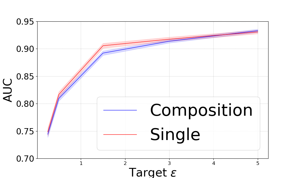
(a) Single-Shot Re-Design

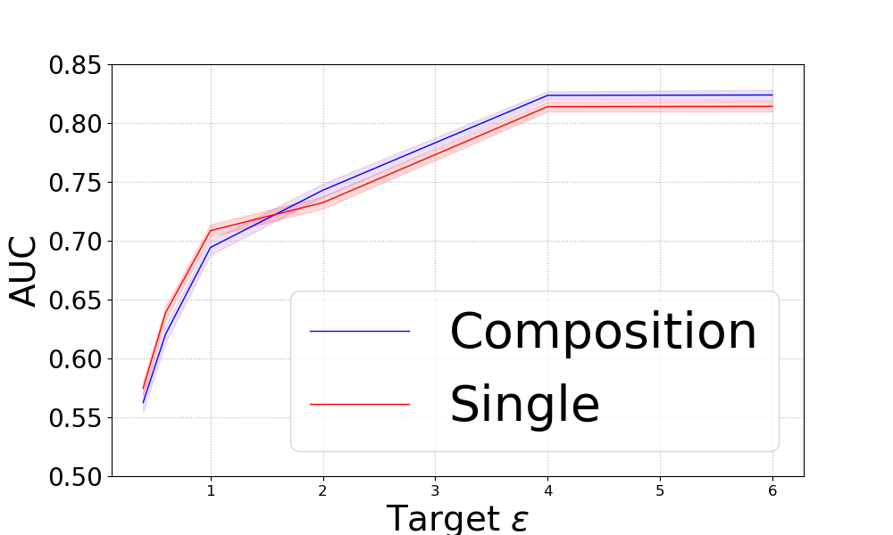
(b) Copula Perturbation

Figure 1: (a) shows five tests with fixed $\delta_{g}=\delta_{i}=0.02$: $\epsilon^{1}_{g}=0.25$ with $\epsilon^{1}_{i}=0.05$, $\epsilon^{2}_{g}=0.25$ with $\epsilon^{2}_{i}=0.1$, $\epsilon^{3}_{g}=1.5$ with $\epsilon^{3}_{i}=0.3$, $\epsilon^{4}_{g}=3$ with $\epsilon^{4}_{i}=0.6$, and $\epsilon^{5}_{g}=5$ with $\epsilon^{5}_{i}=1$, for $i\in\{2,3,4,5\}$. (b) shows six tests with fixed $\delta_{g}=\delta_{i}=0.02$: $\epsilon^{1}_{g}=0.4$ with $\epsilon^{1}_{i}=0.05$, $\epsilon^{2}_{g}=0.6$ with $\epsilon^{2}_{i}=0.1$, $\epsilon^{3}_{g}=1$ with $\epsilon^{3}_{i}=0.18$, $\epsilon^{4}_{g}=2$ with $\epsilon^{4}_{i}=0.3$, $\epsilon^{5}_{g}=4$ with $\epsilon^{5}_{i}=0.6$, and $\epsilon^{5}_{g}=6$ with $\epsilon^{5}_{i}=1$, for $i\in\{1,2,3,4,5\}$.

6 Numerial Experiments

This section presents the copula perturbation and single-shot redesign approaches for the inverse composition of DP in the context of genomic summary statistic sharing. The experiments use a dataset from the 2016 iDASH Workshop on Privacy and Security [32], derived from the 1000 Genomes Project [33], consisting of SNVs from 800 individuals on Chromosome 10. All experiments were conducted on an NVIDIA A40 48G GPU using PyTorch. Detailed experimental settings are provided in the appendix. We consider a mechanism $\mathtt{f}$ that takes as input a dataset $s$ composed of SNVs from 200 individuals and outputs the minor allele frequency (MAF) as summary statistics. Membership information, indicating whether each of the 800 individuals is present ($1$) or absent ($0$) in $s$, is treated as sensitive information. For each realized membership vector, we construct five distinct datasets $\{s_{i}\}_{i=1}^{5}$, where each $s_{i}$ contains a unique set of 300 SNVs from 200 individuals selected from the 800, with $s_{i}\neq s_{j}$ for all $i\neq j$. Thus, the five datasets $\{s_{i}\}_{i=1}^{5}$ share the same sensitive information. We refer to each $f_{i}(s_{i})=f(s_{i})$ as a unique mechanism, and the set $\{f_{i}(s_{i})\}$ represents five different mechanisms accessing datasets with the same sensitive information. Each $(\epsilon_{i},\delta_{i})$-DP mechanism $\mathcal{N}_{i}(s_{i};\psi_{i})=\mathtt{f}_{i}(s_{i})+\mathtt{n}_{i}$, where $\mathtt{n}_{i}$ is Gaussian noise that ensures differential privacy.

We evaluate the strength of privacy protection of the mechanisms by analyzing the performance of membership inference attacks, measured in terms of Area Under the Curve (AUC). Membership inference attacks serve as an auditing tool to quantify the extent of data leakage in machine learning models [34, 35].

In our experiments, we demonstrate the inverse composition for multiple independent differentially private mechanisms using the single-shot re-design and the copula perturbation approaches. Each experiment involves a comparison between the composition of five mechanisms (labeled as “Composition") with the target cumulative privacy loss bound $(\epsilon_{g},\delta_{g})$, implemented by the inverse composition, and the $(\epsilon_{g},\delta_{g})$-CP of a single mechanism (labeled as “Single"). The purpose of these comparisons is to show that the $(\epsilon_{g},\delta_{g})$-CP achieved through the inverse composition of five mechanisms results in a privacy loss similar to that of a single mechanism with $(\epsilon_{g},\delta_{g})$-CP. This comparison is assessed in terms of membership inference attacks, which is a common auditing tool for quantifying data leakage in machine learning models [34, 35]. Thus, the similar performance of the membership inference attacks indicates the similar strength of privacy protection.

Single-shot re-design

We use $800$ individuals with $1000$ SNVs of each individual for the experiments of single-shot re-design. The privacy loss function $\ell_{p}$ used in the experiments is the cross-entropy loss. We use one neural network (termed Defender) to train $\phi_{1}$ to solve (11), where the constraint $\sigma\in\operatorname*{arg\,min}\nolimits_{\sigma^{\prime}}\textup{PriL}\left(\sigma^{\prime},\psi_{1};\theta,\ell_{p}\right)$ is tackled by another neural network (termed Attacker).

Copula perturbation

We use $800$ individuals with $300$ SNVs of each individual for the experiments of copula perturbation. The privacy loss function $\ell_{p}$ used in the experiments is the cross-entropy loss. We use one neural network (termed Defender) to generate $\epsilon_{\mathtt{c}}$ to solve (10). Similar to the single-shot re-design, we use the neural network (termed Attacker) to train the best response $\sigma\in\operatorname*{arg\,min}\nolimits_{\sigma^{\prime}}\textup{PriL}\left(\sigma^{\prime},\epsilon,\delta;\theta,\ell_{p}\right)$.

In the experiments, we train a neural network to simulate the constraint $\sigma\in\operatorname*{arg\,min}\nolimits_{\sigma^{\prime}}\textup{PriL}\left(\cdot\right)$ in both (10) and (11). For the single-shot re-design approach, we consider four mechanisms $\{\mathcal{N}_{i}(\psi_{i})\}_{i=2}^{5}$, each satisfying $(\epsilon_{i},\delta_{i})$-DP. The re-design approach chooses a $\psi_{1}$ to optimize (11) by training a neural network. Figure 1(a) shows the results for five different target $\epsilon_{g}$ values with fixed $\delta_{g}=0.02$, demonstrating that the single-shot re-design effectively performs inverse composition to achieve the target DP under composition. For the copula perturbation approach, we consider five mechanisms $\{\mathcal{N}_{i}(\psi_{i})\}_{i=1}^{5}$, each satisfying $(\epsilon_{i},\delta_{i})$-DP. We train a neural network to generate $\epsilon_{\mathtt{c}}$ for a fixed $\delta_{\mathtt{c}}=0.02$ by solving (10) to obtain $C^{\mathtt{g}}_{\rho}(\epsilon_{\mathtt{c}},\delta_{\mathtt{c}})$ with $\rho=0.5$. Two mechanisms, $\mathcal{N}_{1}(\psi_{1})$ and $\mathcal{N}_{2}(\psi_{2})$, are perturbed using $C^{\mathtt{g}}_{\rho}(\epsilon_{\mathtt{c}},\delta_{\mathtt{c}})$. Figure 1(b) presents the results for six different target $\epsilon_{g}$ values with fixed $\delta_{g}=0.02$, showing that copula perturbation effectively performs inverse composition to achieve the target DP under composition.

7 Conclusion

This paper introduces confounding privacy (CP), extending differential privacy (DP) and Pufferfish privacy (PP) by modeling the probabilistic relationship between sensitive information and dataset output. We demonstrate that while CP remains intact under composition, traditional DP bounds underestimate privacy loss in the CP framework. We propose a novel inverse composition framework to optimally implement a target privacy bound under composition. Two methods of inverse composition are proposed for DP mechanisms. Experimental results validate the effectiveness of our approach to implement target privacy bounds under the composition of DP.

Appendix A CP As Single-Point DP

Consider that the prior knowledge $\theta_{S}\in\Theta_{S}$ is a uniform distribution (or other non-informative prior) over $\mathcal{S}$, and $\mathcal{Q}$ is a set of pairs of adjacent states denoted by $s\simeq s^{\prime}$, where $s$ and $s^{\prime}$ differ in only one entry. Thus, in this case, the sensitive information is an entry of a state, where the relationship between the sensitive information and the state is deterministic. Then, $(\epsilon,\delta)$-CP is a notion of $(\epsilon,\delta)$-differential privacy when we treat the dataset $x$ as some intermediate terms in the probabilistic pipeline from the state to the output.

When we consider adjacent states with subjective priors, the CP framework also mathematically coincides with the Bayesian differential privacy (BDP).

Definition 11 ($(\epsilon_{\omega},\delta_{\omega})$-Bayesian Differential Privacy [36]).

A randomized mechanism $\mathcal{M}:\mathcal{X}\mapsto\mathcal{Y}$ is $(\epsilon_{\omega},\delta_{\omega})$-Bayesian differentially private ($(\epsilon_{\omega},\epsilon_{\omega})$-BDP) with $\epsilon_{\omega}\geq 0$ and $\delta_{\omega}\in[0,1]$, if for any $x\simeq x^{\prime}$ differing in a single entry $z\sim\omega$, we have

$$\textup{Pr}\left[\mathcal{M}(x)\in\widehat{\mathcal{Y}}\right]\leq e^{\epsilon_{\omega}}\textup{Pr}\left[\mathcal{M}(x^{\prime})\in\widehat{\mathcal{Y}}\right]+\delta_{\omega},\forall\widehat{\mathcal{Y}}\subseteq\mathcal{Y},$$

where the probability is taken over the randomness of the output response $y$ and the data entry $z$.

The notion of BDP enjoys many properties of the standard DP [36], including post-processing, composition, and group privacy. The core idea of BDP lies in defining typical scenarios. A scenario is considered as typical when all sensitive data is drawn from the same distribution [36]. This is motivated by the fact that many machine learning models are often designed and trained for specific data distributions, and such prior knowledge is usually known by the attackers. The BDP framework adjusts the noise according to the data distribution and can provide a better expected privacy guarantee.

In the general CP framework, we treat the entire state as sensitive information and consider the probability space over all states, while the BDP only considers the space over a single differing entry. Since the common data entries of the adjacent datasets are assumed to be known by the (worst-case) attacker, these common entries do not impact the distributions of the mechanism. In addition, both standard DP and BDP consider independent data. That is, the privacy guarantees by DP and BDP do not consider the correlation between data entries. Therefore, we can mathematically treat the CP framework as the BDP framework when the virtual dataset (that contains sensitive entry) is a single-point dataset and the true dataset $x$ is some intermediate term that is not publicly observable. However, such a single-point (B)DP equivalence is valid only when there is one mechanism. When multiple CP mechanisms are composed, this equivalence fails (See Section Composition for more detail).

Appendix B Bound-Consistent Privacy Loss

The ordering of privacy strengths, as quantified by the privacy parameters $(\epsilon,\delta)$, is consistently reflected in the ordering of the expected privacy loss across all bound-consistent privacy loss (BCPL) functions. Specifically, if one mechanism $\mathcal{M}_{1}(\gamma_{1})$ is more privacy than another mechanism $\mathcal{M}_{2}(\gamma_{2})$ based on their $(\epsilon,\delta)$ values, then the expected privacy loss for $\mathcal{M}_{1}(\gamma_{1})$ is smaller than that for $\mathcal{M}_{2}(\gamma_{2})$, regardless of which BCPL function is used (as long as it is BCPL). Suppose that $\mathcal{M}_{1}(\gamma_{1})$ and $\mathcal{M}_{2}(\gamma_{2})$ are $(\epsilon,\delta)$-CP and $(\hat{\epsilon},\hat{\delta})$-CP, respectively. Then, for any two BCPL functions $\ell_{p}$ and $\ell^{\prime}_{p}$, such that $\Gamma^{\theta}\left[L_{\epsilon,\delta},\ell_{p}\right]\subseteq\Gamma^{\theta}\left[\epsilon,\delta\right]$ and $\Gamma^{\theta}\left[L_{\hat{\epsilon},\hat{\delta}},\ell_{p}\right]\subseteq\Gamma^{\theta}\left[\hat{\epsilon},\hat{\delta}\right]$, and $\Gamma^{\theta}\left[L_{\epsilon,\delta},\ell^{\prime}_{p}\right]\subseteq\Gamma^{\theta}\left[\epsilon,\delta\right]$ and $\Gamma^{\theta}\left[L_{\hat{\epsilon},\hat{\delta}},\ell^{\prime}_{p}\right]\subseteq\Gamma^{\theta}\left[\hat{\epsilon},\hat{\delta}\right]$, the following hold:

• Suppose $\delta=\hat{\delta}$. Then, the following statements are equivalent.

  • $\epsilon\leq\hat{\epsilon}$.

  • $\textup{E}_{\textup{min}}\left[\ell_{p};\gamma_{1},\theta\right]\geq\textup{E}_{\textup{min}}\left[\ell_{p};\gamma_{2},\theta\right]$.

  • $\textup{E}_{\textup{min}}\left[\ell^{\prime}_{p};\gamma_{1},\theta\right]\geq\textup{E}_{\textup{min}}\left[\ell^{\prime}_{p};\gamma_{2},\theta\right]$.

• Suppose $\epsilon=\hat{\epsilon}$. Then, the following statements are equivalent.

  • $\delta\leq\hat{\delta}$.

  • $\textup{E}_{\textup{min}}\left[\ell_{p};\gamma_{1},\theta\right]\geq\textup{E}_{\textup{min}}\left[\ell_{p};\gamma_{2},\theta\right]$.

  • $\textup{E}_{\textup{min}}\left[\ell^{\prime}_{p};\gamma_{1},\theta\right]\geq\textup{E}_{\textup{min}}\left[\ell^{\prime}_{p};\gamma_{2},\theta\right]$.

Here,

$$\textup{E}_{\textup{min}}\left[\ell_{p};\gamma,\theta\right]\equiv\min\left\{\min_{(s_{0},s_{1})\in\mathcal{Q}}\textup{PriL}\left(\sigma^{*},\gamma,\theta;\ell_{p}\right)\middle|\sigma^{*}\in\Sigma^{\theta}_{s_{0},s_{1}}[\gamma;\ell_{p}]\right\}.$$

The alignment between the ordering of privacy strength and the ordering of the minimum attainable (ex-ante) expected BCPL leads to a corresponding alignment in the ordering of accuracy for the optimal inference strategies under a given BCPL. That is, a more (resp. less) informative mechanism leads to a more (resp. less) accurate optimal inference for any given BCPL. Consequently, Bayesian inference emerges as one of the optimal inference strategies because it maximally exploits the informativeness provided by a given mechanism and prior. In addition, the minimum expected privacy loss value is unique when the loss function is BCPL. We provide two prominent classes of loss functions that are bound-consistent privacy loss that this work particularly focuses on. Simplified notations are used for the ease of exposition.

B.1 Class 1: Joint-Convex and Strict-Convex in Prediction (JCSCP) Loss Functions

A loss function $\ell_{p}(s,\hat{s})$ belongs to the class of Joint-Convex and Strict-Convex in Prediction (JCSCP) functions if it satisfies two key properties:

1. Joint Convexity: The function $\ell_{p}(s,\hat{s})$ is convex in both $s$ and $\hat{s}$ when considered together. This means that the loss function does not create local minima other than the global minimum in its domain, ensuring that any convex combination of points in the domain results in a loss that does not exceed the corresponding convex combination of their losses.

2. Strict Convexity in Prediction: The function $\ell_{p}(s,\hat{s})$ is strictly convex in $\hat{s}$. Formally, for any $s$ and for all $\hat{s}_{1}\neq\hat{s}_{2}$ and $0<\alpha<1$, the following inequality holds:

   $$\ell_{p}(s,\alpha\hat{s}_{1}+(1-\alpha)\hat{s}_{2})<\alpha\ell_{p}(s,\hat{s}_{1})+(1-\alpha)\ell_{p}(s,\hat{s}_{2}).$$

   This property guarantees that the loss function has a unique minimum with respect to $\hat{s}$, thus promoting precise predictions.

Example 1: Mean Squared Error (MSE)

The Mean Squared Error (MSE) is a quintessential example of a symmetric loss function. It is defined as:

$$\ell_{p}(s,\hat{s})=(s-\hat{s})^{2}$$

To demonstrate its symmetry, consider any given values of $s$ and $\hat{s}$. The loss function evaluates as:

$$\ell_{p}(s,\hat{s})=(s-\hat{s})^{2}$$

and

$$\ell_{p}(s,2s-\hat{s})=\left(s-(2s-\hat{s})\right)^{2}=\left(\hat{s}-s\right)^{2}=(s-\hat{s})^{2}.$$

Since the loss remains identical under this transformation, MSE is indeed symmetric, reflecting its impartial treatment of overestimation and underestimation errors.

Example 2: Regularized Squared Error

An example of a JCSCP loss function is the regularized squared error, given by:

$$\ell_{p}(s,\hat{s})=(s-\hat{s})^{2}+\lambda\hat{s}^{2},$$

where $\lambda>0$ is a regularization parameter that penalizes large predictions.

• Convexity: The term $(s-\hat{s})^{2}$ is convex in $\hat{s}$, as it represents a parabolic curve. The regularization term $\lambda\hat{s}^{2}$ is also convex in $\hat{s}$ since it too is a quadratic function. Since the sum of convex functions is convex, $\ell_{p}(s,\hat{s})$ is convex in $\hat{s}$.

• Strict Convexity in $\hat{s}$: The presence of the quadratic term $\lambda\hat{s}^{2}$ ensures strict convexity in $\hat{s}$. This strict convexity means that the loss function will have a unique minimizer with respect to the prediction $\hat{s}$, making it particularly useful in optimization problems where uniqueness of the solution is desirable.

B.2 Class 2: Proper Scoring Rules

A scoring rule $\textup{Score}(p,s)$ is considered proper if it incentivizes truthful probability predictions by minimizing the expected score when the predicted distribution $p$ matches the true distribution $q$. Mathematically, $\textup{Score}(p,s)$ is proper if for all predicted distributions $p$ and true distributions $q$:

$$\mathbb{E}_{s\sim q}[\textup{Score}(q,s)]\leq\mathbb{E}_{s\sim q}[\textup{Score}(p,s)].$$

The scoring rule is strictly proper if equality holds if and only if $p=q$, meaning the minimum expected score is achieved uniquely when the predicted probabilities exactly match the true probabilities. When using a proper scoring rule as the loss function, the minimum expected loss value is unique. This uniqueness arises because the expected loss is minimized only when the predicted distribution matches the true distribution, and this minimum value cannot be matched by any other incorrect distribution.

Example: Logarithmic Score (Log-Score)

The logarithmic score, often referred to as log-loss in the context of classification tasks, is a classic example of a proper scoring rule. It is defined as:

$$\textup{Score}(p,s)=-\log p(s),$$

where $p(s)$ is the predicted probability assigned to the true class $s$.

For binary classification, where $s\in\{0,1\}$, the log-score operates as follows:

• If the true class is $s=1$, the score is $\textup{Score}(p,1)=-\log p(1)$.

• If the true class is $s=0$, the score is $\textup{Score}(p,0)=-\log p(0)$.

The log-score is minimized when the predicted probabilities $p(1)$ and $p(0)$ are aligned with the actual underlying probabilities of the classes, thereby ensuring that truthful predictions are rewarded. This property makes log-loss a powerful tool in probabilistic classification and model evaluation. An instantiation of the log-score loss function is the cross-entropy loss.

Appendix C More on Copula Perturbation and Inverse Composition

C.1 Copula Perturbation

In the copula perturbation, we use $N\left(0,\mathtt{w}^{2}\left(\frac{\mathtt{C}_{\textup{sen}}}{\epsilon_{\mathtt{c}}}\right)^{2}\right)$ with $\mathtt{w}\geq 2\log(2/\delta_{\mathtt{c}})$ and $N(0,1)$ to generate the latent variables $z_{1}$ and $z_{2}$, respectively. Additionally, the copula perturbation employs a mechanism $\tilde{\eta}_{S}$ to impose dependence on the state, where the latent variable $z_{1}$ acts as Gaussian noise to perform output perturbation for $\tilde{\eta}_{S}$. As a result, this Gaussian copula achieves $(\epsilon_{\mathtt{s}},\delta_{\mathtt{c}})$-CP. This procedure allows the copula to influence the total cumulative privacy loss of the mechanisms under composition.

This copula perturbation is straightforward to implement, with state dependence solely captured by the deterministic mechanism $\tilde{\eta}_{S}$, which is entirely independent of the design of the underlying distributions of the Gaussian copula. Alternative approaches to copula perturbation exist. For instance, we could select the parameters (e.g., correlation coefficient $\rho$, mean, or variance) of the bivariate Gaussian distribution that serves as the copula framework based on the states, thereby introducing state dependence into the copula itself.

In the process of the pseudo-random sample generation, we jointly sample noises $v_{1}$ and $v_{2}$ to perturb the selected two mechanisms $\mathcal{M}_{1}(\gamma_{1})$ and $\mathcal{M}_{2}(\gamma_{2})$. However, the copula perturbation does not require these two mechanisms to operate simultaneously. In particular, the key requirement is that the noise used to perturb each of $\mathcal{M}_{1}(\gamma_{1})$ and $\mathcal{M}_{2}(\gamma_{2})$ is generated through the pseudo-random sample generation process.

C.2 Inverse Composition

By using copula perturbation, the inverse composition aims to implement a target privacy budget $(\epsilon_{g},\delta_{g})$ while ensuring that each individual mechanism $\mathcal{M}_{i}(\gamma_{i})$ preserves the predetermined $(\epsilon_{i},\delta_{i})$-CP. The core of the inverse composition lies in using the bound-consistent privacy loss (BCPL) function, which ensures that the posterior distributions induced by the underlying probability distributions of the individual mechanisms, the copula, and the prior comply with the constraints specified by the convex set (8). By straightforwardly extending the conditions of Proposition 1 to multiple outputs observed under composition, we conclude that the composition of the given mechanisms with the optimal copula satisfies $(\epsilon_{g},\delta_{g})$-CP. By definition of bound-consistent privacy loss (BCPL), if the composition of $\{\mathcal{M}_{i}(\gamma_{i})\}^{k}_{i=1}$ is $(\epsilon_{g},\delta_{g})$-CP for one certain BCPL function $\ell_{p}$, it is also $(\epsilon_{g},\delta_{g})$-CP for another BCPL function $\ell_{p}$.

However, for a given group of mechanisms $\{\mathcal{M}_{i}(\gamma_{i})\}^{k}_{i=1}$, where each $\mathcal{M}_{i}(\gamma_{i})$ is $(\epsilon_{i},\delta_{i})$-CP, not every arbitrary target $(\epsilon_{g},\delta_{g})$ can be implemented. In particular, for a fixed $\delta_{g}$, any $\epsilon_{g}<\textup{OPT}_{\delta_{g}}(\textup{PL}(b_{s_{0}}\|b_{s_{1}}))$ cannot be implemented, where $\textup{OPT}_{\delta_{g}}(\textup{PL}(b_{s_{0}}\|b_{s_{1}}))$ represents the tightest epsilon value under composition without any perturbation. This limitation arises because, when preserving each individual mechanism’s $(\epsilon_{i},\delta_{i})$-CP, it is impossible that the total cumulative privacy loss can be strictly less than $\textup{OPT}_{\delta_{g}}(\textup{PL}(b_{s_{0}}\|b_{s_{1}}))$. However, if the preservation of individual mechanisms’ predetermined local privacy is not required, then the inverse composition by re-designing all mechanisms can technically implement all feasible target privacy budgets.

The application of inverse composition to standard DP is straightforward. Inverse composition using copula perturbation effectively transforms DP under composition into CP by introducing dependencies between independent mechanisms, with the dependence entirely controlled by the copula. When considering the privacy loss of copula-perturbed mechanisms under composition, the copula perturbation plays a role in partially designing the cumulative privacy loss of these mechanisms. The single-shot re-design can be seen as a special case of copula perturbation, where the privacy loss of a single mechanism is directly designed, albeit at the expense of violating the predetermined local privacy guarantee for that mechanism.

Appendix D Proof of Lemma 1

Since the privacy loss function $\ell_{p}$ is convex and strictly convex with respect to the inference conclusion, the minimum expected privacy loss is unique. Therefore, if $\ell_{p}$ is utilized, then for any $(\epsilon,\delta)$-CP mechanism $\mathcal{M}(\gamma^{*})$, there exists an attainable bound $L_{\epsilon,\delta}$ such that $\gamma^{*}\in\Gamma^{\theta}[L_{\epsilon,\delta},\ell_{p}]$. Furthermore, by the definition of bound-consistent privacy loss functions, if $\mathcal{M}(\gamma^{*})$ is a $(\epsilon,\delta)$-CP mechanism, then for any bound-consistent privacy loss function $\hat{\ell}_{p}$, there exists a corresponding bound $\hat{L}_{\epsilon,\delta}$.

∎

Appendix E Proof of Lemma 2

Lemma 2 is a corollary of Proposition 2.4 and Proposition 2.12 of [18]. To prove Lemma 2, we first need to show that there exists uniformly most powerful test for the problem:

• $H_{0}$: with prior knowledge $\theta$, the state is $s_{0}$.

• $H_{1}$: with prior knowledge $\theta$, the state is $s_{1}$.

It is straightforward to see that this is a simple binary hypothesis testing problem. Hence, Neyman-Pearson lemma implies that the likelihood-ratio test is the UMP test. Therefore, for any significance level $\alpha\in[0,1]$, there is

$$\beta^{\alpha}=\inf\nolimits_{\phi}\left\{\beta_{\phi}:\alpha_{\phi}\leq\alpha\right\},$$

such that $\alpha=\mathbb{E}[\phi|H_{0},\gamma]$ and $\beta^{\alpha}=1-\mathbb{E}[\phi|H_{1},\gamma]$. Therefore, the mechanism $\mathcal{M}(\gamma)$ is $f$-differentially private (Definition 2.3 of [18]). Then, by Proposition 2.4 of [18], $\mathcal{M}(\gamma)$ is also $f^{*}$-differentially private, where $f^{*}(y)=\sup\nolimits_{0\leq\alpha^{\prime}\leq 1}y\alpha^{\prime}-f(\alpha^{\prime})$. Then, we obtain $\delta(\epsilon)=1+f^{*}(-e^{\epsilon})$ from Proposition 2.12 of [18].

∎

Appendix F Proof of Lemma 3

Consider the following hypothesis testing:

• $H_{0}$: with prior knowledge $\theta$, the state is $s_{0}$.

• $H_{1}$: with prior knowledge $\theta$, the state is $s_{1}$.

Under the composition, given any $\vec{y}=(y_{1},y_{2})$, the likelihood ratio is given by

$$\textup{LR}(y_{1},y_{2})=\frac{\textup{L}(y_{1},y_{2}|H_{0})}{\textup{L}(y_{1},y_{2}|H_{1})},$$

where

$$\textup{L}(y_{1},y_{2}|H_{\ell})=\int\limits_{x}\prod_{i=1}^{k}\gamma_{i}(y_{i}|x)\frac{p_{\theta}(s_{\ell},x)}{p_{\theta_{S}}(s_{\ell})}dx,$$

for $\ell\in\{0,1\}$, which is well-defined. Then, the proof of part (i) follows Lemma 2.

∎

Appendix G Proofs of Proposition 1

We prove Proposition 1 by the following steps. By using Lemma 4 shown below, we first obtain that

$$\textup{J}\left(s\middle|y;\gamma,\theta\right)\geq e^{-\epsilon}p_{\theta_{S}}(s),\mathbb{E}\left[\frac{\textup{J}\left(S\middle|y;\gamma,\theta\right)}{p_{\theta_{S}}(S)}\right]\leq\delta e^{\epsilon}$$

implies

$$\textup{Pr}\left[e^{-\epsilon}\leq\frac{\textup{J}\left(S\middle|y;\gamma,\theta\right)}{p_{\theta_{S}}(S)}\leq e^{\epsilon}\right]\geq 1-\delta,$$ (12)

for any $y\in\mathcal{Y}$. The probability in (12) is taken over the randomness of $S\sim\textup{J}(\cdot|y;\gamma,\theta)$. Then, if $Y\sim\gamma(\cdot|s_{0})$, it holds that

$$\textup{Pr}_{Y\sim\gamma(\cdot|s_{0})}\left[e^{-\epsilon}\leq\frac{\textup{J}\left(S\middle|Y;\gamma,\theta\right)}{p_{\theta_{S}}(S)}\leq e^{\epsilon}\right]\geq 1-\delta.$$ (13)

Next, Lemma 5 implies that

$$e^{-\epsilon}\leq\frac{\textup{J}\left(s^{\prime}\middle|y;\gamma,\theta\right)}{p_{\theta_{S}}(s^{\prime})}\leq e^{\epsilon},$$ (14)

for $s^{\prime}\in\{s_{0},s_{1}\}\in\mathcal{Q}$ is equivalent to

$$\textup{Pr}\left[y\in\mathcal{W}\middle|s_{0};\theta,\gamma\right]\leq e^{\epsilon}\textup{Pr}\left[y\in\mathcal{W}\middle|s_{1};\theta,\gamma\right],$$

for all $(s_{0},s_{1})\in\mathcal{Q}$, $\mathcal{W}\subset\mathcal{Y}$. Thus, by (13), we have

$$\textup{Pr}_{Y\sim\gamma(\cdot|s_{0})}\left[\frac{\textup{Pr}\left[Y\in\mathcal{W}\middle|s_{0};\theta,\gamma\right]}{\textup{Pr}\left[Y\in\mathcal{W}\middle|s_{1};\theta,\gamma\right]}\leq e^{\epsilon}\right]\geq 1-\delta.$$ (15)

Finally, Lemma 6 shows that (15) implies

$$\textup{Pr}\left[y\in\mathcal{W}\middle|s_{0};\theta,\gamma\right]\leq e^{\epsilon}\textup{Pr}\left[y\in\mathcal{W}\middle|s_{1};\theta,\gamma\right]+\delta.$$

Therefore, we can conclude the sufficiency of the conditions given by Lemma 1.

Lemma 4.

Let $F:\mathcal{Y}\mapsto\Delta(\mathcal{S})$ be any conditional probability mass or density function, and let $p_{\theta_{S}}\in\Delta(\mathcal{S})$ be any prior distribution. For any $\epsilon\geq 0$ and $\delta\in[0,1)$, if

$$F(s|y)\geq e^{-\epsilon}p_{\theta_{S}}(s)\textup{ and }\mathbb{E}\left[\frac{F\left(S\middle|y\right)}{p_{\theta_{S}}(S)}\right]\leq\delta e^{\epsilon},$$

where the expectation is taken over the randomness of $S\sim F(\cdot|y)$, then

$$\textup{Pr}\left[e^{-\epsilon}\leq\frac{F(S|y)}{p_{\theta_{S}}(S)}\leq e^{\epsilon}\right]\geq 1-\delta,$$

for any $s\in\{s_{0},s_{1}\}\in\mathcal{Q}$, $y\in\mathcal{Y}$.

Proof.

First, $F(s|y)\geq e^{-\epsilon}p_{\theta_{S}}(s)$ implies

$$\textup{Pr}\left[e^{-\epsilon}\leq\frac{F(s|y)}{p_{\theta_{S}}(s)}\leq e^{\epsilon}\right]=1-\textup{Pr}\left[\frac{F(s|\vec{y}_{[k]})}{P_{\theta_{S}}(s)}\geq e^{\epsilon}\right].$$

By Markov’s inequality, we have

$$\textup{Pr}\left[\frac{F(s|\vec{y}_{[k]})}{P_{\theta_{S}}(s)}\geq e^{\epsilon}\right]\leq\frac{\mathbb{E}\left[\frac{F(s|\vec{y}_{[k]})}{P_{\theta_{S}}(s)}\right]}{e^{\epsilon}}.$$

Since $\mathbb{E}\left[\frac{F\left(S\middle|y\right)}{p_{\theta_{S}}(S)}\right]\leq\delta e^{\epsilon}$, we have

$$\textup{Pr}\left[\frac{F(s|\vec{y}_{[k]})}{P_{\theta_{S}}(s)}\geq e^{\epsilon}\right]\leq\delta.$$

Therefore, $\textup{Pr}\left[e^{-\epsilon}\leq\frac{F(s|\vec{y}_{[k]})}{P_{\theta_{S}}(s)}\leq e^{\epsilon}\right]\geq 1-\delta$. ∎

Lemma 5.

A mechanism is $(\epsilon,\delta)$-CP if and only if the posterior belief $\textup{J}(\cdot;\gamma,\theta)$ satisfies

$$e^{-\epsilon}\leq\frac{\textup{J}\left(s^{\prime}\middle|y;\gamma,\theta\right)}{p_{\theta_{S}}(s^{\prime})}\leq e^{\epsilon},$$

for all $s^{\prime}\in\{s_{0},s_{1}\}\in\mathcal{Q}$.

Lemma 5 directly extends Claim 3 of [1] to the general confounding privacy. Since $(\epsilon,\delta)$-CP can be viewed as a single-point DP, the proof of Lemma 5 follows Claim 3 of [1].

Lemma 6.

Given $\theta\in\Theta$, if

$$\textup{Pr}_{Y\sim\gamma(\cdot|s_{0})}\left[\frac{\textup{Pr}\left[Y\in\mathcal{W}\middle|s_{0};\theta,\gamma\right]}{\textup{Pr}\left[Y\in\mathcal{W}\middle|s_{1};\theta,\gamma\right]}\leq e^{\epsilon}\right]\geq 1-\delta,$$ (16)

for all $\mathcal{W}\subseteq\mathcal{Y}$, $(s_{0},s_{1})\in\mathcal{Q}$, $\epsilon\geq 0$, $\delta\in[0,1)$, then we have

$$\textup{Pr}\left[y\in\mathcal{W}\middle|s_{0};\theta,\gamma\right]\leq e^{\epsilon}\textup{Pr}\left[y\in\mathcal{W}\middle|s_{1};\theta,\gamma\right]+\delta.$$

The condition (16) is equivalent to the strong Bayesian DP introduced by [36]. By treating the CP as a single-point DP, Lemma 6 can be proved in the similar way as Proposition 1 of [36].

∎

Appendix H Proof of Theorem 2

Both Theorems 1 and 2 show that the tightest privacy bound under the optimal composition of DP underestimates the actual cumulative privacy loss of CP. We prove these two theorems together in this section.

For ease of exposition, we restrict attention to the composition of two individual mechanisms without loss of generality. Consider two mechanisms $\mathcal{M}_{1}(\gamma_{1})$ and $\mathcal{M}_{2}(\gamma_{2})$ that are $(\epsilon_{1},\delta_{1})$-CP and $(\epsilon_{2},\delta_{2})$-CP, respectively. Let $\mathcal{N}_{i}(\psi_{i})$ be induced by $\mathcal{M}_{i}(\gamma_{i})$ for $i\in\{1,2\}$. Recall that the density function $\psi_{i}$ is given by

$$\psi_{i}(y_{i}|s)=\int\limits_{x}\gamma_{i}(y_{i}|x)\frac{p_{\theta}(s,x)}{p_{\theta_{S}}(s)}dx,$$

which is induced by $\gamma_{i}$ and $\theta$. Let

$$\mathtt{D}_{1,2}(y_{1},y_{2}|s)=\psi_{1}(y_{1}|s)\psi_{2}(y_{2}|s).$$

In addition, the density function associated with $\mathcal{M}(\gamma_{[2]})$ is give by

$$\mathtt{D}_{[2]}(y_{1},y_{2}|s)=\int\limits_{x}\prod_{i=1}^{2}\gamma_{i}(y_{i}|x)\frac{p_{\theta}(s,x)}{p_{\theta_{S}}(s)}dx.$$

We adopt the general notation of trade-off function given by Definition 2.1 of [18].

Definition 12 (trade-off function).

Let $\alpha_{\phi}$ and $\beta_{\phi}$ be the Type-I and Type-II errors given any rejection rule $\phi$, respectively. For any two probability distributions $P$ and $Q$ on the same space, define the trade-off function $T(P,Q):[0,1]\to[0,1]$ as

$$T(P,Q)(\alpha)=\inf\{\beta_{\phi}:\alpha_{\phi}\leq\alpha\},$$

where the infimum is taken over all (measurable) rejection rules.

The following Proposition 4 shows that for any $\gamma_{[2]}$, $\mathtt{D}_{[2]}$ is more informative than $\mathtt{D}_{1,2}$ about the state in the sense of Blackwell [37, 38].

Proposition 4.

For any $(s_{1},s_{0})\in\mathcal{Q}$ and $\alpha\in[0,1]$, we have

$$T(\mathtt{D}_{[2]}(\cdot|s_{0}),\mathtt{D}_{[2]}(\cdot|s_{1}))\leq T(\mathtt{D}_{1,2}(\cdot|s_{0}),\mathtt{D}_{1,2}(\cdot|s_{1})),$$

where the equality holds if and only if $\mathtt{D}_{[2]}=\mathtt{D}_{1,2}$.

The proof of Proposition 4 depends on Lemmas 7 and 8. In particular, Lemma 7 shows that the Bayesian inference based on $\mathtt{D}_{[2]}$ leads to a smaller expected cross-entropy loss than that based on $\mathtt{D}_{1,2}$. Lemma 8 establishes an equivalence between the ordering of expected cross-entropy losses and the Blackwell’s ordering of informativeness. Thus, by Lemmas 7 and 8, we can prove Proposition 4.

H.1 Detailed Proofs

By Bayes’ rule, construct the posterior distributions as follows:

$$\textup{J}_{1,2}(s|y_{1},y_{2})=\frac{\mathtt{D}_{1,2}(y_{1},y_{2}|s)p_{\theta_{S}}(s)}{\textup{P}_{1,2}(y_{1},y_{2})},$$

$$\textup{J}_{[2]}(s|y_{1},y_{2})=\frac{\mathtt{D}_{[2]}(y_{1},y_{2}|s)p_{\theta_{S}}(s)}{\textup{P}_{[2]}(y_{1},y_{2})},$$

where $\textup{P}_{1,2}(y_{1},y_{2})=\int_{s}\mathtt{D}_{1,2}(y_{1},y_{2}|s)p_{\theta_{S}}(s)ds$ and $\textup{P}_{[2]}(y_{1},y_{2})=\int_{s}\mathtt{D}_{[2]}(y_{1},y_{2}|s)p_{\theta_{S}}(s)ds$ are the marginal likelihoods.

For any attack model $\mathcal{A}(\sigma)$ with $\sigma:\mathcal{Y}_{1}\times\mathcal{Y}_{2}\mapsto\Delta(\mathcal{S})$, the expected CEL induced by $\{\gamma_{1},\gamma_{2},\theta\}$ is given by

$$\textup{CEL}\left(\sigma\right)=-\int\limits_{s,x}p_{\theta}(s,x)\int\limits_{y_{1},y_{2}}\prod_{i=1}^{2}\gamma_{i}(y_{i}|x)\log\sigma(s|y_{1},y_{2})dxdsdy_{[2]}.$$

Lemma 7.

The following holds

$$\textup{CEL}\left(\textup{J}_{[2]}\right)\leq\textup{CEL}\left(\textup{J}_{1,2}\right),$$

where the equality holds if and only if $\textup{J}_{[2]}=\textup{J}_{1,2}$.

Proof.

We consider the difference between the expected CELs

$$\textup{CEL}\left(\textup{J}_{1,2}\right)-\textup{CEL}\left(\textup{J}_{[2]}\right)=-\int\limits_{s,x}p_{\theta}(s,x)\int\limits_{y_{1},y_{2}}\prod_{i=1}^{2}\gamma_{i}(y_{i}|x)\times\log\frac{\textup{J}_{[2]}(s|y_{1},y_{2})}{\textup{J}_{1,2}(s|y_{1},y_{2})}dxdsdy_{[2]}.$$

By definitions of $\mathtt{D}_{[2]}$ and $\textup{J}_{[2]}$, we have

$$\textup{J}_{[2]}(s|y_{1},y_{2})\textup{P}_{[2]}(y_{1},y_{2})=\int\limits_{x}\prod_{i=1}^{2}\gamma_{i}(y_{i}|x)p_{\theta}(s,x)dx.$$

Then, we can rewrite the difference $\textup{CEL}\left(\textup{J}_{1,2}\right)-\textup{CEL}\left(\textup{J}_{[2]}\right)$ using the definition of Kullback–Leibler (KL) divergence between $\textup{J}_{[2]}$ and $\textup{J}_{1,2}$ as

$$\textup{CEL}\left(\textup{J}_{1,2}\right)-\textup{CEL}\left(\textup{J}_{[2]}\right)=\textup{KL}\left(\textup{J}_{[2]}\|\textup{J}_{1,2}\right),$$

where

$$\textup{KL}\left(\textup{J}_{[2]}\|\textup{J}_{1,2}\right) =\int_{s}\int_{y_{1},y_{2}}\textup{J}_{[2]}(s|y_{1},y_{2})\times\log\frac{\textup{J}_{[2]}(s|y_{1},y_{2})}{\textup{J}_{1,2}(s|y_{1},y_{2})}\textup{P}_{[2]}(y_{1},y_{2})dy_{1}dy_{2}ds.$$

Since $\textup{KL}\left(\textup{J}_{[2]}\|\textup{J}_{1,2}\right)\geq 0$, where the equality holds if and only if $\textup{J}_{[2]}=\textup{J}_{1,2}$, it follows that

$$\textup{CEL}\left(\textup{J}_{[2]}\right)\leq\textup{CEL}\left(\textup{J}_{1,2}\right).$$

∎

Lemma 8.

Let $\mathcal{A}(\sigma)$ with $\sigma:\mathcal{Y}_{1}\times\mathcal{Y}_{2}\mapsto\Delta(\mathcal{S})$ be any attack model. Let $\textup{J}_{[2]}$ and $\textup{J}_{1,2}$ be the posterior distributions induced by $\mathtt{D}_{[2]}$ and $\mathtt{D}_{1,2}$, respectively. Then, the following two statements are equivalent

• $\textup{CEL}\left(\textup{J}_{[2]}\right)\leq\textup{CEL}\left(\textup{J}_{1,2}\right)$.

• For any $(s_{1},s_{0})\in\mathcal{Q}$ and $\alpha\in[0,1]$,

  $$T(\mathtt{D}_{[2]}(\cdot|s_{0}),\mathtt{D}_{[2]}(\cdot|s_{1}))\leq T(\mathtt{D}_{1,2}(\cdot|s_{0}),\mathtt{D}_{1,2}(\cdot|s_{1})).$$

The equality holds if and only if $\mathtt{D}_{[2]}=\mathtt{D}_{1,2}$.

Proof.

By Theorem 1 of [38], we have the part (ii) of Lemma 8 is equivalent to the following:

• There exists a randomized mechanism $\mathtt{Proc}:\mathcal{Y}_{1}\times\mathcal{Y}_{2}\mapsto\mathcal{Z}$ such that $\mathtt{D}_{1,2}(s_{0})=\mathtt{Proc}\left(\mathtt{D}_{[2]}(s_{0})\right)$ and $\mathtt{D}_{1,2}(s_{1})=\mathtt{Proc}\left(\mathtt{D}_{[2]}(s_{1})\right)$ for all $(s_{0},s_{1})\in\mathcal{Q}$.

Then, by Theorem 10 in [37] (see also Theorem 2.10 in [18] and Theorem 2.5 in [5]), we establish the equivalence of parts (i) and (ii) of Lemma 8. ∎

Recall that a function $f:[0,1]\mapsto[0,1]$ is a symmetric trade-off function if it is convex, continuous, non-increasing, satisfies $f(\alpha)\leq 1-\alpha$, and $f(\alpha)=\inf\{t\in[0,1]:f(t)\leq\alpha\}$ for $\alpha\in[0,1]$ [18]. The convex conjugate of $f$ is defined by

$$f^{*}(y)=\sup\nolimits_{0\leq\alpha^{\prime}\leq 1}y\alpha^{\prime}-f(\alpha^{\prime}).$$

Let $\epsilon^{*}(\delta_{g})=\textup{OPT}\left(\mathcal{N}(\psi_{[2]}),\delta_{g}\right)$ for any $\delta_{g}\in[0,1)$, where $\psi_{[2]}$ is induced by $\gamma_{[2]}$. In addition, let $\delta_{[2]}(\epsilon_{g})=1+f^{*}_{[2]}(-e^{\epsilon_{g}})$ and $\delta_{1,2}(\epsilon_{g})=1+f^{*}_{1,2}(-e^{\epsilon_{g}})$, for any $\epsilon_{g}\geq 0$. When $\mathtt{D}_{[2]}\neq\mathtt{D}_{1,2}$, Proposition 4 implies $T(\mathtt{D}_{[2]}(\cdot|s_{0}),\mathtt{D}_{[2]}(\cdot|s_{1}))<T(\mathtt{D}_{1,2}(\cdot|s_{0}),\mathtt{D}_{1,2}(\cdot|s_{1}))$. Then, $f_{[2]}(\alpha)<f_{1,2}(\alpha)$ for all $\alpha\in[0,1]$, which implies that for any fixed $\epsilon_{g}$ and $\epsilon$, we have $\delta_{[2]}(\epsilon)>\delta_{1,2}(\epsilon)$. Suppose that $\delta_{[2]}(\epsilon_{[2]})=\delta_{1,2}(\epsilon_{1,2})$. Then, $f^{*}_{[2]}(-e^{\epsilon^{[2]}_{g}})=f^{*}_{1,2}(-e^{\epsilon^{1,2}_{g}})$. Since both $f_{[2]}$ and $f_{1,2}$ are convex, continuous, and non-increasing functions, their convex conjugates are concave, continuous, and non-decreasing functions. In addition, since $\delta_{[2]}(\epsilon)>\delta_{1,2}(\epsilon)$ for all $\epsilon\geq 0$, in order to get $\delta_{[2]}(\epsilon_{[2]})=\delta_{1,2}(\epsilon_{1,2})$, we must have $\epsilon_{[2]}>\epsilon_{1,2}$. Therefore, we finish the proof of Theorem 1 (Appendix E).

Theorem 1 confirms the following parts of Theorem 2:

• If $\mathcal{L}_{c_{s_{0}}\|c_{s_{1}}}(\vec{Y})\neq 0$, then

  $$\underline{\textup{OPT}}_{\delta_{g}}(s_{0},s_{1})<\textup{OPT}_{\delta_{g}}(\textup{PL}(b_{s_{0}}\|b_{s_{1}}))$$

  $$\textup{and }\underline{\delta}^{\epsilon_{g}}(s_{0},s_{1})<\delta^{\epsilon_{g}}(\textup{PL}(b_{s_{0}}\|b_{s_{1}})).$$

The second inequalities

$$\textup{OPT}_{\delta_{g}}(\textup{PL}(b_{s_{0}}\|b_{s_{1}}))\leq\overline{\textup{OPT}}_{\delta_{g}}(s_{0},s_{1})$$

$$\delta^{\epsilon_{g}}(\textup{PL}(b_{s_{0}}\|b_{s_{1}}))\leq\overline{\delta}^{\epsilon_{g}}(s_{0},s_{1})$$

arise from the fact that, in the PLRV given by (6), the copula-dependent random variable $\mathcal{L}_{c_{s_{0}}\|c_{s_{1}}}(\vec{Y})$ is correlated with the set $\{\mathcal{L}_{\psi_{i}^{s_{0}}\|\psi_{i}^{s_{1}}}(Y_{i})\}_{i=1}^{k}$, where each element of $\{\mathcal{L}_{\psi_{i}^{s_{0}}\|\psi_{i}^{s_{1}}}(Y_{i})\}_{i=1}^{k}$ is independent of the others. Consequently, even when each $\psi_{i}$ attains the bounds of its probabilistic indistinguishability, the copula may not attain its own bound. The maximum privacy loss ($\overline{\textup{OPT}}_{\delta_{g}}(s_{0},s_{1})$ or $\overline{\delta}^{\epsilon_{g}}(s_{0},s_{1})$) occurs when all the individual mechanisms and the copula term achieve their respective bounds of probabilistic indistinguishability is maximized.

∎

Proof of Theorem 3

Part (i) of Theorem 3 demonstrates that our modified Gaussian copula $C^{\mathtt{g}}_{\rho}(\Xi_{1},\Xi_{2};\epsilon_{\mathtt{c}},\delta_{\mathtt{c}})$ is a valid copula which retains the marginals as $\gamma_{1}$ and $\gamma_{2}$. Part (ii) of Theorem 3 shows that the conservative upper bound given by Theorem 2 can be calculated using Theorem 1.5 of [6], given $(\epsilon_{\mathtt{c}},\delta_{\mathtt{c}})$ that parameterized the Gaussian distribution of $Z_{1}$ in the process $\textup{PsedR}_{\rho}(\cdot|\Xi_{1},\Xi_{2})$. For simplicity, we omit $\epsilon_{\mathtt{c}},\delta_{\mathtt{c}}$ and write $C^{\mathtt{g}}_{\rho}(\Xi_{1},\Xi_{2})$.

H.2 Proof of Part (i)

Part (i) of Theorem 3 can be proved by showing that

$$C^{\mathtt{g}}_{\rho}(V_{1},V_{2}|\Xi_{1},\Xi_{2})=\Phi_{\rho^{\prime}}\left(F_{1}^{-1}(\Xi_{1}(V_{1})),F_{\rho}^{-1}(\Xi_{2}(V_{2}))\right)$$

is indeed a valid copula for any $\rho^{\prime}\in(-1,1)$ and $\rho\in(-1,1)\backslash\{0\}$ so that the marginals of the joint distribution $\overline{\textup{PR}}(Z_{1},Z_{2}|\Xi_{1},\Xi_{2})$ are $\Xi_{1}$ and $\Xi_{2}$. Let

$$C^{g}_{\rho}(U_{1},U_{2})=\Phi_{\rho^{\prime}}\left(F^{-1}_{1}(U1),F^{-1}_{\rho}(U_{2})\right).$$

$C^{\mathtt{g}}_{\rho}(V_{1},V_{2}|\Xi_{1},\Xi_{2})$ is a valid copula if the following holds.

• $C^{g}_{\rho}(U_{1},U_{2})$ is a valid joint CDF.

• $C^{g}_{\rho}(U_{1},U_{2})$ has uniform marginals,

where (a) directly follows the definition of $\Phi_{\rho^{\prime}}$ which is the joint CDF of bivariate Gaussian distribution with zero mean and correlation coefficient $\rho^{\prime}$.

Uniform marginal for $U_{1}$

Given any $s$, the CDF of $z_{1}(s)$ is given by

$$F_{1}(z_{1}(s))=\Phi\left(\frac{z_{1}-\tilde{\eta}_{S}(s)}{\sqrt{\mathtt{var}_{1}}}\right),$$

where $\Phi$ is the CDF of the standard Gaussian distribution, and $\mathtt{var}_{1}=\mathtt{w}^{2}\left(\frac{\mathtt{C}_{\textup{sen}}}{\epsilon_{\mathtt{c}}}\right)^{2}$. By the probability integral transform, $U_{1}=F_{1}(Z_{1}(s))$ is uniformly distributed on $[0,1]$ because $F_{1}$ maps the real line to $[0,1]$ and it is a continuous, strictly increasing function.

Uniform marginal for $U_{2}$

Given any $s$, $F_{\rho}$ is the CDF of the random variable

$$\hat{Z}_{2}(s)=\rho Z_{1}(s)+\sqrt{(}1-\rho^{2})Z_{2},$$

where $Z_{2}\sim N(0,1)$. Hence,

$$F_{\rho}(\hat{z}_{2}(s))=\Phi\left(\frac{\hat{z}_{2}(s)-\rho\tilde{\eta}_{S}(s)}{\sqrt{(}\rho^{2}\mathtt{var}_{1}+(1-\rho^{2}))}\right).$$

Again, by the probability integral transform, $U_{2}=F_{\rho}(\hat{Z}_{2}(s))$ is uniformly distributed on $[0,1]$ since $F_{\rho}$ is a valid CDF mapping $\hat{Z}_{2}(s)$ to a uniform distributed random variable on $[0,1]$.

Therefore, $C^{\mathtt{g}}_{\rho}(V_{1},V_{2}|\Xi_{1},\Xi_{2})$ is a valid copula whose marginal distributions are $\Xi_{1}$ and $\Xi_{2}$. Here, each $\Xi_{i}$ is independently chosen (without considering composition) such that the mechanism $\mathcal{M}_{i}(\gamma_{i})$ is $(\epsilon_{i},\delta_{i})$-CP for $i\in\{1,2\}$. Then, if the attacker only has access to one of these two mechanisms, each $\mathcal{M}_{i}(\gamma_{i})$ of the $C^{\mathtt{g}}_{\rho}(V_{1},V_{2}|\Xi_{1},\Xi_{2})$ perturbed $\{\mathcal{M}_{1}(\gamma_{1}),\mathcal{M}_{2}(\gamma_{2})\}$ maintains $(\epsilon_{i},\delta_{i})$-CP.

H.3 Proof of Part (ii)

Recall that $\mathtt{C}_{\textup{sen}}=\sup_{(s_{1},s_{0})\in\mathcal{Q}}|\tilde{\eta}_{S}(s_{0})-\tilde{\eta}_{S}(s_{1})|$ is the sensitivity of a function $\tilde{\eta}_{S}:\mathcal{S}\mapsto\mathcal{B}$ that releases a univariate output $\tilde{\eta}_{S}(s)$ given the state $s$. Given any state $s\in\mathcal{S}$, let $z_{1}(s)=\tilde{\eta}_{S}(s)+\tilde{z}_{1}$, where $\tilde{z}_{1}$ is drawn from $N\left(0,\mathtt{w}^{2}\left(\frac{\mathtt{C}_{\textup{sen}}}{\epsilon_{\mathtt{c}}}\right)^{2}\right)$ for any $\mathtt{w}\geq 2\log(2/\delta_{\mathtt{c}})$ with $\epsilon_{\mathtt{c}}\geq 0$ and $\delta_{\mathtt{c}}\in[0,1)$. Then, it is straightforward to verify that $z_{1}(s_{0})$ and $z_{1}(s_{1})$ are normally distributed with mean $\tilde{\eta}_{S}(s_{0})$ and $\tilde{\eta}_{S}(s_{1})$, respectively, and a common variance $\mathtt{var}_{1}=\mathtt{w}^{2}\left(\frac{\mathtt{C}_{\textup{sen}}}{\epsilon_{\mathtt{c}}}\right)^{2}$.

For any $s$, let

$$C^{g}_{\rho}(U_{1}(s),U_{2}(s))=\Phi_{\rho^{\prime}}\left(F^{-1}_{1}(U1),F^{-1}_{\rho}(U_{2})\right),$$

where $U_{1}(s)=F_{1}(Z_{1}(s))$ and $U_{2}(s)=F_{\rho}(\hat{Z}_{2}(s))$. By Theorem 4.3 in [2], we can show that $z_{1}(s)$ satisfies $(\epsilon_{\mathtt{c}},\delta_{\mathtt{c}})$-SDP. By the post-processing of DP, $C^{g}_{\rho}(U_{1}(s),U_{2}(s))$ is also $(\epsilon_{\mathtt{c}},\delta_{\mathtt{c}})$-SDP. Here, the formulation $\hat{Z}_{2}(s)=\rho Z_{1}(s)+\sqrt{(}1-\rho^{2})Z_{2}$ is deterministic and a linear combination of $Z_{1}(s)$ and $Z_{2}$, where $\rho\neq-1$ or $1$ that avoiding the degenerate cases. The CDFs are strictly monotone functions. In addition, all the inverse CDFs are assumed to be continuous and well-defined. Therefore, the process $C^{g}_{\rho}(u_{1}(s),u_{2}(s))$ is a deterministic one-to-one mapping (from $(z_{1}(s),z_{2})$). Thus, the parameters $(\epsilon_{\mathtt{c}},\delta_{\mathtt{c}})$ of $C^{g}_{\rho}(u_{1}(s),u_{2}(s))$’s CP are tight given $(z_{1}(s),z_{2})$.

Recall (after Equation (6)) that we can define the privacy loss random variable

$$\widehat{\mathcal{L}}_{s_{0}|s_{1}}(U_{1}(s),U_{2}(s),Y_{1},Y_{2})\equiv\mathcal{L}_{\hat{c}_{s_{0}}\|\hat{c}_{s_{1}}}(U_{1}(s),U_{2}(s))+\sum^{2}_{i=1}\mathcal{L}_{\psi_{i}^{s_{0}}\|\psi_{i}^{s_{1}}}(Y_{i}),$$

where $\hat{c}_{s}=c^{\mathtt{g}}_{\rho}(U_{1}(s),U_{2}(s))$. Hence, if we treat the copula as the independent mechanism accessing to any dataset related to $s$, then we can obtain the conservative bound

$$\overline{\textup{OPT}}_{\delta_{g}}(s_{0},s_{1})=\textup{OptComp}((\epsilon_{\mathtt{c}},\delta_{\mathtt{c}}),\epsilon_{1},\delta_{1}),\epsilon_{2},\delta_{2}),\delta_{g}),$$

for any $(s_{1},s_{0})\in\mathcal{Q}$, $\delta_{g}\in[0,1)$, where OptComp is given by Theorem 1.5 of [6].

∎

sectionProof of Proposition 2

For simplicity, we omit $(\epsilon_{\mathtt{c}},\delta_{\mathtt{c}})$ and write $C^{\mathtt{g}}_{\rho}(\Xi_{1},\Xi_{2};\epsilon_{\mathtt{c}},\delta_{\mathtt{c}})$.

Recall that $\psi_{i}:\mathcal{S}\mapsto\Delta(\mathcal{Y}_{i})$ is the density function induced by $\gamma_{i}$ and $\theta$, and $\Psi_{i}$ is the corresponding CDF.

Suppose that the noise perturbation $y_{i}=\mathtt{A}(v_{i})$ and $\mathtt{A}$ is strictly increasing. Then, $\mathtt{A}^{-1}(Y_{i})\leq v_{i}$ is equivalent to $Y_{i}\leq\mathtt{A}(v_{i})$. Thus, we have

$$\Xi_{i}(v_{i})=\textup{Pr}\left(\mathtt{A}^{-1}(Y_{i})\leq v_{i}\right)=\Psi_{i}(\mathtt{A}(v_{i})|s).$$

Suppose that the noise perturbation $y_{i}=\mathtt{A}(v_{i})$ and $\mathtt{A}$ is strictly decreasing. Then, $\mathtt{A}^{-1}(Y_{i})\leq v_{i}$ is equivalent to $Y_{i}\geq\mathtt{A}(v_{i})$. Thus, we have

$$\Xi_{i}(v_{i})=\textup{Pr}\left(\mathtt{A}^{-1}(Y_{i})\geq v_{i}\right)=1-\Psi_{i}(\mathtt{A}(v_{i})|s).$$

Therefore, when the invertible $\mathtt{A}$ is strictly increasing and strictly decreasing, respectively, we have

$$\widehat{C}^{\mathtt{g}}_{\rho^{\prime}}(V_{1},V_{2}|\Xi_{1},\Xi_{2};s)=\Phi_{\rho^{\prime}}\left(F_{1}^{-1}(\Psi_{1}(\mathtt{A}(V_{1})|s)),F_{\rho}^{-1}(\Psi_{2}(\mathtt{A}(V_{2})|s))\right)$$

and

$$\widetilde{C}^{\mathtt{g}}_{\rho^{\prime}}(V_{1},V_{2}|\Xi_{1},\Xi_{2};s)=\Phi_{\rho^{\prime}}\left(F_{1}^{-1}(1-\Psi_{1}(\mathtt{A}(V_{1})|s)),F_{\rho}^{-1}(1-\Psi_{2}(\mathtt{A}(V_{2})|s))\right).$$

In addition, let $\widehat{c}^{\mathtt{g}}_{\rho^{\prime}}\left(V_{1},V_{2}\middle|s\right)$ and $\widetilde{c}^{\mathtt{g}}_{\rho^{\prime}}\left(V_{1},V_{2}\middle|s\right)$ be the corresponding copula densities.

For the two mechanisms $\mathcal{M}_{1}(\gamma_{1})$ and $\mathcal{M}_{2}(\gamma_{2})$ perturbed by $C^{\mathtt{g}}_{\rho}(V_{1},V_{2}|\Xi_{1},\Xi_{2})$, let $\Psi_{[2]}(Y_{1},Y_{2}|s,C^{\mathtt{g}}_{\rho})$ denote the joint CDF of the outputs $Y_{1}$ and $Y_{2}$.

Lemma 9.

The following holds.

• If invertible $\mathtt{A}$ is strictly increasing, then

  $$\Psi_{[2]}(Y_{1},Y_{2}|s,C^{\mathtt{g}}_{\rho})=\widehat{C}^{\mathtt{g}}_{\rho}(Y_{1},Y_{2}|\Xi_{1},\Xi_{2};s).$$

• If invertible $\mathtt{A}$ is strictly decreasing, then

  $$\Psi_{[2]}(Y_{1},Y_{2}|s,C^{\mathtt{g}}_{\rho})=\widetilde{C}^{\mathtt{g}}_{\rho}(Y_{1},Y_{2}|\Xi_{1},\Xi_{2};s).$$

Proof.

Suppose invertible $\mathtt{A}$ is strictly increasing. Then,

$$\Psi_{[2]}(y_{1},y_{2}|s,C^{\mathtt{g}}_{\rho}) =\textup{Pr}\left(Y_{1}\leq y_{1},Y_{2}\leq y_{2}\right)=\textup{Pr}\left(\mathtt{A}(V_{1})\leq y_{1},\mathtt{A}(V_{1})\leq y_{2}\right)$$

$$=\textup{Pr}\left(V_{1}\leq\mathtt{A}^{-1}(y_{1}),V_{2}\leq\mathtt{A}^{-1}(y_{2})\right).$$

In addition, $V_{i}\leq\mathtt{A}^{-1}(y_{i})$ is equivalent to $Y_{i}=\mathtt{A}(V_{i})\leq y_{i}$, which yields

$$\Xi_{i}(\mathtt{A}^{-1}(y_{i}))=\textup{Pr}\left(V_{i}\leq\mathtt{A}^{-1}(y_{i})\right)=\Psi_{i}(y_{i}),$$

for all $i\in[k]$. Since $V_{1}$ and $V_{2}$ has joint CDF $C^{\mathtt{g}}_{\rho}(\cdot|\Xi_{1},\Xi_{2})$, we have

$$\Psi_{[2]}(y_{1},y_{2}|s,C^{\mathtt{g}}_{\rho})=C^{\mathtt{g}}_{\rho}(\mathtt{A}^{-1}(y_{1}),\mathtt{A}^{-1}(y_{2})|\Xi_{1},\Xi_{2}) =\Phi_{\rho^{\prime}}\left(F_{1}^{-1}(\Psi_{1}(\mathtt{A}(\mathtt{A}^{-1}(y_{1}))|s)),F_{\rho}^{-1}(\Psi_{2}(\mathtt{A}(\mathtt{A}^{-1}(y_{2}))|s))\right)$$

$$=\Phi_{\rho^{\prime}}\left(F_{1}^{-1}(\Psi_{1}(y_{1}|s)),F_{\rho}^{-1}(\Psi_{2}(y_{2}|s))\right).$$

A similar procedure can be used to prove (ii). ∎

Lemma 9 shows that the dependency between $Y_{1}$ and $Y_{2}$ due to the copula perturbation can be completely characterized by the same structure $C^{\mathtt{g}}_{\rho^{\prime}}$ as the noises $V_{1}$ and $V_{2}$.

Under the copula perturbation using $C^{\mathtt{g}}_{\rho^{\prime}}$, let $b(\cdot|s;c^{\mathtt{g}}_{\rho^{\prime}})$ denote the joint density. Then,

$$b\left(\vec{Y}\middle|s\right)=c\left(\Psi_{[2]}(Y_{1},Y_{2}|s,C^{\mathtt{g}}_{\rho}),\Psi_{3}(Y_{3}|s),\dots,\Psi_{k}\left(Y_{k}\middle|s\right)\middle|s\right)\psi_{[2]}(Y_{1},Y_{2}|s,C^{\mathtt{g}}_{\rho})\prod^{k}\nolimits_{i=3}\psi_{i}\left(Y_{i}|s\right)$$

$$=c\left(\Psi_{[2]}(Y_{1},Y_{2}|s,C^{\mathtt{g}}_{\rho}),\Psi_{3}(Y_{3}|s),\dots,\Psi_{k}\left(Y_{k}\middle|s\right)\middle|s\right)c^{\mathtt{g}}_{\rho}(y_{1},y_{2}|s)\prod^{k}\nolimits_{i=1}\psi_{i}\left(Y_{i}|s\right),$$

where $\psi_{[2]}$ is the joint density of the joint CDF $\Psi_{[2]}$. For any $(s_{0},s_{1})\in\mathcal{Q}$, define

$$\widehat{\mathcal{L}}_{s_{0}\|s_{1}}(Y_{1},Y_{2};\widehat{c}^{\mathtt{g}}_{\rho})\equiv\log\frac{\widehat{c}^{\mathtt{g}}_{\rho}(\Psi_{1}(Y_{1}|s_{1}),\Psi_{2}(Y_{2}|s_{1})|\epsilon_{\mathtt{c}},\delta_{\mathtt{c}})}{\widetilde{c}^{\mathtt{g}}_{\rho}(\Psi_{1}(Y_{1}|s_{0}),\Psi_{2}(Y_{2}|s_{0})|\epsilon_{\mathtt{c}},\delta_{\mathtt{c}})},$$

and

$$\widetilde{\mathcal{L}}_{s_{0}\|s_{1}}(Y_{1},Y_{2};\widetilde{c}^{\mathtt{g}}_{\rho})\equiv\log\frac{\widetilde{c}^{\mathtt{g}}_{\rho}(\Psi_{1}(Y_{1}|s_{1}),\Psi_{2}(Y_{2}|s_{1})|\epsilon_{\mathtt{c}},\delta_{\mathtt{c}})}{\widetilde{c}^{\mathtt{g}}_{\rho}(\Psi_{1}(Y_{1}|s_{0}),\Psi_{2}(Y_{2}|s_{0})|\epsilon_{\mathtt{c}},\delta_{\mathtt{c}})}.$$

Then, by the product rule for Logarithms, we can separate the copula $\widehat{c}^{\mathtt{g}}_{\rho}$ and $\widetilde{c}^{\mathtt{g}}_{\rho}$ and obtain

$$\widetilde{\mathcal{L}}_{b_{s_{0}}\|b_{s_{1}}}(\vec{Y};C^{\mathtt{g}}_{\rho})=\mathcal{L}_{b_{s_{0}}\|b_{s_{1}}}(\vec{Y})+\widehat{\mathcal{L}}_{s_{0}\|s_{1}}(Y_{1},Y_{2};\widehat{c}^{\mathtt{g}}_{\rho}),$$

and

$$\widetilde{\mathcal{L}}_{b_{s_{0}}\|b_{s_{1}}}(\vec{Y};C^{\mathtt{g}}_{\rho})=\mathcal{L}_{b_{s_{0}}\|b_{s_{1}}}(\vec{Y})+\widetilde{\mathcal{L}}_{s_{0}\|s_{1}}(Y_{1},Y_{2};\widetilde{c}^{\mathtt{g}}_{\rho}).$$

∎

sectionProof of Proposition 3, Corollaries 1 and 2

The key role of the BCPL in the inverse composition is that the optimizations indirectly impose the constraints in the convex set (8) for the posterior distributions induced by the underlying probability distributions of the mechanisms and the copula. Then, by trivially extending the conditions in Proposition 1 to multiple outputs as observations under composition, we can conclude that the composition of the given mechanisms with the optimal Gaussian copula is $(\epsilon_{g},\delta_{g})$-CP.

Here, we prove that Bayesian inference is one of the optimal inference strategies when the privacy loss functions belong to the classes of JCSCP and the proper scoring rules. For simplicity, let $\gamma^{\mathtt{g}}_{[k]}(y_{[k]}|x,s)$ denote the effective joint density given $\gamma_{[k]}$ and the Gaussian copula $C^{\mathtt{g}}_{\rho}$ that perturbs $\mathcal{M}_{1}(\gamma_{1})$ and $\mathcal{M}_{2}(\gamma_{2})$.

The posterior distribution induced by $\{\{\gamma_{i}\}^{k}_{i=1}\theta,C^{\mathtt{g}}_{\rho}\}$ is given by

$$\textup{J}^{\mathtt{g}}_{[k]}\left(s\middle|y_{[k]}\right)=\frac{\mathtt{D}^{\mathtt{g}}_{[k]}(y_{[k]}|s)p_{\theta_{S}}(s)}{\textup{P}^{\mathtt{g}}_{[k]}(y_{[k]})}$$

where

$$\mathtt{D}^{\mathtt{g}}_{[k]}(y_{[k]}|s)=\int\limits_{x}c^{\mathtt{g}}_{\rho}(y_{1},y_{2}|s)\prod_{i=1}^{k}\gamma_{i}(y_{i}|x)\frac{p_{\theta}(s,x)}{p_{\theta_{S}}(s)}dx,$$

and $\textup{P}^{\mathtt{g}}_{[k]}(y_{[k]})$ is the corresponding marginal likelihood.

H.4 JCSCP Loss Function

Suppose that $\ell_{p}$ is a JCSCP function. For any $s$ and $y_{[k]}$, define

$$\textup{PL}(\hat{s},y_{[k]})\equiv\mathbb{E}\left[\ell_{p}(S,\hat{s})\middle|y\right]=\int_{s}\ell_{p}(s,\hat{s})\textup{J}^{\mathtt{g}}_{[k]}\left(s\middle|y_{[k]}\right)ds.$$

By Jensen’s inequality, we have

$$\ell_{p}(\int_{s}s\textup{J}^{\mathtt{g}}_{[k]}\left(s\middle|y_{[k]}\right)ds,\hat{s})\leq\int_{s}\ell_{p}(s,\hat{s})\textup{J}^{\mathtt{g}}_{[k]}\left(s\middle|y_{[k]}\right),$$

which implies that for a fixed prediction $\hat{s}$, the expected loss $\textup{PL}(\hat{s},y_{[k]})$ is minimized when $s$ is replaced by its posterior-expected value $\mathbb{E}[S|y_{[k]}]$. For any $\sigma:\prod^{k}_{i=1}\mathcal{Y}_{i}\mapsto\Delta(\mathcal{S})$, by applying the strict convexity in $\hat{s}$, we know that

$$\textup{R}(\sigma,y_{[k]})\equiv\int_{\hat{s}}\textup{PL}(\hat{s},y_{[k]})\sigma(\hat{s}|y_{[k]})d\hat{s},$$

is minimized when $\sigma(\hat{s}|y_{[k]})=\textup{J}^{\mathtt{g}}_{[k]}\left(\hat{s}\middle|y_{[k]}\right)$ because the posterior distribution $\textup{J}^{\mathtt{g}}_{[k]}\left(s\middle|y_{[k]}\right)$ correctly weights each possible prediction $\hat{s}$ according to the true distribution of $s$ given $y$. In addition, $\sigma(\hat{s}|y_{[k]})=\textup{J}^{\mathtt{g}}_{[k]}\left(\hat{s}\middle|y_{[k]}\right)$ also minimizes $\textup{PriL}\left(\sigma,\epsilon_{\mathtt{c}},\delta_{\mathtt{c}};\theta,\ell_{p}\right)$ because

$$\textup{PriL}\left(\sigma^{\prime},\epsilon_{\mathtt{c}},\delta_{\mathtt{c}};\theta,\ell_{p}\right)=\int_{y_{[k]}}\textup{R}(\sigma,y_{[k]})\textup{P}_{[k]}(y_{[k]})dy_{[k]}.$$

In addition, since $\ell_{p}(s,\hat{s})$ is strictly convex in $\hat{s}$, the function $\frac{\partial}{\partial\hat{s}}\textup{PL}(\hat{s},y_{[k]})$ is also strictly convex in $\hat{s}$, which implies that the minimizer of $\frac{\partial}{\partial\hat{s}}\textup{PL}(\hat{s},y_{[k]})$ is unique. Therefore, $\textup{J}^{\mathtt{g}}_{[k]}\in\Sigma^{\epsilon_{g},\delta_{g}}$. Then, by trivially extending the conditions in Proposition 1 to multiple outputs as observations under composition, we can conclude that the composition of the given mechanisms with the optimal Gaussian copula is $(\epsilon_{g},\delta_{g})$-CP

H.5 Proper Scoring Rules: Cross-Entropy Loss

Consider that $\ell_{p}$ is the cross-entropy loss. For any attack model $\mathcal{A}(\sigma)$ with $\sigma:\prod^{k}_{i=1}\mathcal{Y}_{i}\mapsto\Delta(\mathcal{S})$, the expected CEL induced by $\{\{\gamma_{i}\}^{k}_{i=1}\theta,C^{\mathtt{g}}_{\rho}\}$ is given by

$$\textup{CEL}^{\mathtt{g}}\left(\sigma\right)=-\int\limits_{s,x}p_{\theta}(s,x)\int\limits_{y_{[k]}}\Big{(}c^{\mathtt{g}}_{\rho}(y_{1},y_{2}|s)\prod_{i=1}^{k}\gamma_{i}(y_{i}|x)\log\sigma(s|y_{[k]})dxdsdy_{[k]}\Big{)}.$$

Consider the difference

$$\textup{CEL}^{\mathtt{g}}\left(\sigma\right)-\textup{CEL}^{\mathtt{g}}\left(\textup{J}^{\mathtt{g}}_{[k]}\right)=-\int\limits_{s,x}p_{\theta}(s,x)\int\limits_{y_{[k]}}\Big{(}c^{\mathtt{g}}_{\rho}(y_{1},y_{2}|s)\prod_{i=1}^{k}\gamma_{i}(y_{i}|x)\log\frac{\textup{J}^{\mathtt{g}}_{[k]}(s|y_{[k]})}{\sigma(s|y_{[k]})}dxdsdy_{[k]}\Big{)}.$$

By definitions of $\textup{J}^{\mathtt{g}}_{[k]}$ and $\mathtt{D}^{\mathtt{g}}_{[k]}$, we have

$$\textup{J}^{\mathtt{g}}_{[k]} \left(s\middle|y_{[k]}\right)\textup{P}^{\mathtt{g}}_{[k]}(y_{[k]})=\int\limits_{x}c^{\mathtt{g}}_{\rho}(y_{1},y_{2}|s)\prod_{i=1}^{k}\gamma_{i}(y_{i}|x)p_{\theta}(s,x)dx.$$

Then,

$$\textup{CEL}^{\mathtt{g}}\left(\sigma\right)-\textup{CEL}^{\mathtt{g}}\left(\textup{J}^{\mathtt{g}}_{[k]}\right)=\textup{KL}\left(\textup{J}^{\mathtt{g}}_{[k]}\|\sigma\right),$$

where

$$\textup{KL}\left(\textup{J}^{\mathtt{g}}_{[k]}\|\sigma\right) =\int_{s}\int_{y_{1},y_{2}}\textup{J}_{[k]}(s|y_{[k]})\log\frac{\textup{J}_{[k]}(s|y_{[k]})}{\sigma(s|y_{[k]})}\textup{P}_{[k]}(y_{[k]})dy_{[k]}ds$$

is the KL divergence. Since the KL divergence is non-negative where zero is achieved if and only if $\sigma(s|y_{[k]})=\textup{J}_{[k]}(s|y_{[k]})$ for all $s$ and $y_{[k]}$, it follows that

$$\textup{CEL}^{\mathtt{g}}\left(\sigma\right)\geq\textup{CEL}^{\mathtt{g}}\left(\textup{J}^{\mathtt{g}}_{[k]}\right).$$

Therefore, $\textup{J}^{\mathtt{g}}_{[k]}\in\operatorname*{arg\,min}\nolimits_{\sigma^{\prime}}\textup{PriL}\left(\sigma^{\prime},\epsilon_{\mathtt{c}},\delta_{\mathtt{c}};\theta,\ell_{p}\right)$ when $\ell_{p}$ is the cross-entropy loss. In addition, $\textup{J}^{\mathtt{g}}_{[k]}\in\Sigma^{\epsilon_{g},\delta_{g}}$. Then, by Proposition 1, we can conclude that the composition of the given mechanisms with the optimal Gaussian copula is $(\epsilon_{g}.\delta_{g})$-CP.

Corollaries 1 and 2 directly follow Proposition 3.

∎

Appendix I Experiment Details

I.1 Network Configurations and Hyperparameters

The Defender neural network is a generative model designed to process membership vectors and generate beacon modification decisions. The input layer is followed by a series of fully connected layers with activation functions applied after each layer. The first and second hidden layers use ReLU activation, while the third hidden layer employs LeakyReLU activation. Layer normalization is applied after the second and third hidden layers. The output layer utilizes a custom ScaledSigmoid activation function, producing a real value in a scaled range determined by this function. The network is trained using the AdamW optimizer with a learning rate of $1.5\times 10^{-5}$ and weight decay of $1.5\times 10^{-5}$. Specific configurations for Defender performing single-shot re-design and copula perturbation are provided in Tables 1 and 2, respectively.

The Attacker neural network is a generative model designed to process beacons and noise, producing membership vectors. The input layer is followed by multiple fully connected layers, each equipped with batch normalization and ReLU activation. The output layer applies a standard sigmoid activation function. All Attacker models were trained using the AdamW optimizer, with a learning rate of $1.0\times 10^{-4}$ and a weight decay of $1.0\times 10^{-4}$. Specific configurations for Attacker when Defender performing single-shot re-design and copula perturbation are provided in Tables 3 and 4, respectively.

Defender	Input Units	Output Units
Input Layer	800	5000
Hidden Layer 1	5000	9000
Hidden Layer 2	9000	3000
Output Layer	3000	1000

Table 1: Defender Neural Network Architecture (Single Re-Design)

Defender	Input Units	Output Units
Input Layer	830	3000
Hidden Layer 1	3000	2000
Hidden Layer 2	2000	1200
Hidden Layer 3	1200	1200
Output Layer	1200	1

Table 2: Defender Neural Network Architecture (Copula Perturbation)

Attacker	Input Units	Output Units
Input Layer	1500	14000
Hidden Layer 1	14000	9500
Hidden Layer 2	9500	4500
Output Layer	4500	800

Table 3: Attacker Neural Network Architecture (Single Re-Design)

Attacker	Input Units	Output Units
Input Layer	1500	31000
Hidden Layer 1	31000	25000
Hidden Layer 2	25000	15000
Output Layer	15000	800

Table 4: Attacker Neural Network Architecture (Copula Perturbation)

I.2 AUC Values with Standard Deviations

Tables 5 and 6 show the AUC values shown in the plots.

Target $\&$ Ind. $\epsilon$	Mechanisms	AUC ± std
$\epsilon_{g}=0.25$, $\epsilon_{i}=0.05$	Composition	0.7441 ± 0.0055
	Single	0.7485 ± 0.0064
$\epsilon_{g}=0.5$, $\epsilon_{i}=0.1$	Composition	0.8093 ± 0.0042
	Single	0.8165 ± 0.0044
$\epsilon_{g}=1.5$, $\epsilon_{i}=0.3$	Composition	0.8921 ± 0.0031
	Single	0.9056 ± 0.0029
$\epsilon_{g}=3$, $\epsilon_{i}=0.6$	Composition	0.9138 ± 0.0031
	Single	0.9175 ± 0.0031
$\epsilon_{g}=5$, $\epsilon_{i}=1$	Composition	0.9330 ± 0.0029
	Single	0.9308 ± 0.0028

Table 5: AUC and standard deviation for single-shot re-design when the target $\delta_{g}$ and each individual $\delta_{i}$ are the same, i.e., $\delta_{g}=\delta_{i}=0.02$, and $\rho=0.5$

Target $\&$ Ind. $\epsilon$	Type	AUC ± std
$\epsilon_{g}=0.4$, $\epsilon_{i}=0.05$	Composition	0.5624 ± 0.0078
	Single	0.5745 ± 0.0060
$\epsilon_{g}=0.6$, $\epsilon_{i}=0.1$	Composition	0.6206 ± 0.0071
	Single	0.6388 ± 0.0053
$\epsilon_{g}=1$, $\epsilon_{i}=0.18$	Composition	0.6943 ± 0.0063
	Single	0.7086 ± 0.0052
$\epsilon_{g}=2$, $\epsilon_{i}=0.3$	Composition	0.7429 ± 0.0055
	Single	0.7324 ± 0.0051
$\epsilon_{g}=4$, $\epsilon_{i}=0.6$	Composition	0.8235 ± 0.0035
	Single	0.8139 ± 0.0042
$\epsilon_{g}=6$, $\epsilon_{i}=1$	Composition	0.8238 ± 0.0043
	Single	0.8142 ± 0.0044

Table 6: AUC and standard deviation for copula perturbation when the target $\delta_{g}$ and each individual $\delta_{i}$ are the same, i.e., $\delta_{g}=\delta_{i}=0.02$, and $\rho=0.5$

References

- [1] Cynthia Dwork, Frank McSherry, Kobbi Nissim, and Adam Smith. Calibrating noise to sensitivity in private data analysis. In Theory of Cryptography: Third Theory of Cryptography Conference, TCC 2006, New York, NY, USA, March 4-7, 2006. Proceedings 3, pages 265–284. Springer, 2006.
- [2] Cynthia Dwork. Differential privacy: getting more for less. In Proc. Int. Cong. Math, volume 6, pages 4740–4761, 2022.
- [3] Daniel Kifer and Ashwin Machanavajjhala. Pufferfish: A framework for mathematical privacy definitions. ACM Transactions on Database Systems (TODS), 39(1):1–36, 2014.
- [4] Damien Desfontaines and Balázs Pejó. Sok: differential privacies. arXiv preprint arXiv:1906.01337, 2019.
- [5] Peter Kairouz, Sewoong Oh, and Pramod Viswanath. The composition theorem for differential privacy. In International conference on machine learning, pages 1376–1385. PMLR, 2015.
- [6] Jack Murtagh and Salil Vadhan. The complexity of computing the optimal composition of differential privacy. In Theory of Cryptography Conference, pages 157–175. Springer, 2015.
- [7] Roger B Nelsen. An introduction to copulas. Springer, 2006.
- [8] Xi He, Ashwin Machanavajjhala, and Bolin Ding. Blowfish privacy: Tuning privacy-utility trade-offs using policies. In Proceedings of the 2014 ACM SIGMOD international conference on Management of data, pages 1447–1458, 2014.
- [9] Shuang Song, Yizhen Wang, and Kamalika Chaudhuri. Pufferfish privacy mechanisms for correlated data. In Proceedings of the 2017 ACM International Conference on Management of Data, pages 1291–1306, 2017.
- [10] Wanrong Zhang, Olga Ohrimenko, and Rachel Cummings. Attribute privacy: Framework and mechanisms. In Proceedings of the 2022 ACM Conference on Fairness, Accountability, and Transparency, pages 757–766, 2022.
- [11] Theshani Nuradha and Ziv Goldfeld. Pufferfish privacy: An information-theoretic study. IEEE Transactions on Information Theory, 2023.
- [12] Cynthia Dwork, Guy N Rothblum, and Salil Vadhan. Boosting and differential privacy. In 2010 IEEE 51st Annual Symposium on Foundations of Computer Science, pages 51–60. IEEE, 2010.
- [13] Salil Vadhan and Tianhao Wang. Concurrent composition of differential privacy. In Theory of Cryptography: 19th International Conference, TCC 2021, Raleigh, NC, USA, November 8–11, 2021, Proceedings, Part II 19, pages 582–604. Springer, 2021.
- [14] Xin Lyu. Composition theorems for interactive differential privacy. Advances in Neural Information Processing Systems, 35:9700–9712, 2022.
- [15] Salil Vadhan and Wanrong Zhang. Concurrent composition theorems for differential privacy. In Proceedings of the 55th Annual ACM Symposium on Theory of Computing, pages 507–519, 2023.
- [16] Ilya Mironov. Rényi differential privacy. In 2017 IEEE 30th computer security foundations symposium (CSF), pages 263–275. IEEE, 2017.
- [17] Borja Balle and Yu-Xiang Wang. Improving the gaussian mechanism for differential privacy: Analytical calibration and optimal denoising. In International Conference on Machine Learning, pages 394–403. PMLR, 2018.
- [18] Jinshuo Dong, Aaron Roth, and Weijie J Su. Gaussian differential privacy. Journal of the Royal Statistical Society Series B: Statistical Methodology, 84(1):3–37, 2022.
- [19] David M Sommer, Sebastian Meiser, and Esfandiar Mohammadi. Privacy loss classes: The central limit theorem in differential privacy. Proceedings on Privacy Enhancing Technologies, 2019(2):245–269.
- [20] Antti Koskela, Joonas Jälkö, and Antti Honkela. Computing tight differential privacy guarantees using fft. In International Conference on Artificial Intelligence and Statistics, pages 2560–2569. PMLR, 2020.
- [21] Mark Bun and Thomas Steinke. Concentrated differential privacy: Simplifications, extensions, and lower bounds. In Theory of Cryptography Conference, pages 635–658. Springer, 2016.
- [22] Martin Abadi, Andy Chu, Ian Goodfellow, H Brendan McMahan, Ilya Mironov, Kunal Talwar, and Li Zhang. Deep learning with differential privacy. In Proceedings of the 2016 ACM SIGSAC conference on computer and communications security, pages 308–318, 2016.
- [23] Yu-Xiang Wang, Borja Balle, and Shiva Prasad Kasiviswanathan. Subsampled rényi differential privacy and analytical moments accountant. In The 22nd international conference on artificial intelligence and statistics, pages 1226–1235. PMLR, 2019.
- [24] Sivakanth Gopi, Yin Tat Lee, and Lukas Wutschitz. Numerical composition of differential privacy. Advances in Neural Information Processing Systems, 34:11631–11642, 2021.
- [25] Yuqing Zhu, Jinshuo Dong, and Yu-Xiang Wang. Optimal accounting of differential privacy via characteristic function. In International Conference on Artificial Intelligence and Statistics, pages 4782–4817. PMLR, 2022.
- [26] Antti Koskela, Marlon Tobaben, and Antti Honkela. Individual privacy accounting with gaussian differential privacy. arXiv preprint arXiv:2209.15596, 2022.
- [27] Cynthia Dwork and Moni Naor. On the difficulties of disclosure prevention in statistical databases or the case for differential privacy. Journal of Privacy and Confidentiality, 2(1), 2010.
- [28] Cynthia Dwork. Differential privacy: A survey of results. In International conference on theory and applications of models of computation, pages 1–19. Springer, 2008.
- [29] Stephan R Sain. The nature of statistical learning theory, 1996.
- [30] M Sklar. Fonctions de répartition à n dimensions et leurs marges. In Annales de l’ISUP, volume 8, pages 229–231, 1959.
- [31] Thomas Steinke. Composition of differential privacy & privacy amplification by subsampling. arXiv preprint arXiv:2210.00597, 2022.
- [32] Haixu Tang, X Wang, Shuang Wang, and Xiaoqian Jiang. Idash privacy and security workshop, 2016.
- [33] 1000 Genomes Project Consortium et al. A global reference for human genetic variation. Nature, 526(7571):68, 2015.
- [34] Samuel Yeom, Irene Giacomelli, Matt Fredrikson, and Somesh Jha. Privacy risk in machine learning: Analyzing the connection to overfitting. In 2018 IEEE 31st computer security foundations symposium (CSF), pages 268–282. IEEE, 2018.
- [35] Santiago Zanella-Beguelin, Lukas Wutschitz, Shruti Tople, Ahmed Salem, Victor Rühle, Andrew Paverd, Mohammad Naseri, Boris Köpf, and Daniel Jones. Bayesian estimation of differential privacy. In International Conference on Machine Learning, pages 40624–40636. PMLR, 2023.
- [36] Aleksei Triastcyn and Boi Faltings. Bayesian differential privacy for machine learning. In International Conference on Machine Learning, pages 9583–9592. PMLR, 2020.
- [37] David Blackwell et al. Comparison of experiments. In Proceedings of the second Berkeley symposium on mathematical statistics and probability, volume 1, page 26, 1951.
- [38] Henrique de Oliveira. Blackwell’s informativeness theorem using diagrams. Games and Economic Behavior, 109:126–131, 2018.