Analytical and Empirical Study of Herding Effects in Recommendation Systems
Abstract.
Online rating systems are often used in numerous web or mobile applications, e.g., Amazon and TripAdvisor, to assess the ground-truth quality of products. Due to herding effects, the aggregation of historical ratings (or historical collective opinion) can significantly influence subsequent ratings, leading to misleading and erroneous assessments. We study how to manage product ratings via rating aggregation rules and shortlisted representative reviews, for the purpose of correcting the assessment error. We first develop a mathematical model to characterize important factors of herding effects in product ratings. We then identify sufficient conditions (via the stochastic approximation theory), under which the historical collective opinion converges to the ground-truth collective opinion of the whole user population. These conditions identify a class of rating aggregation rules and review selection mechanisms that can reveal the ground-truth product quality. We also quantify the speed of convergence (via the martingale theory), which reflects the efficiency of rating aggregation rules and review selection mechanisms. We prove that the herding effects slow down the speed of convergence while an accurate review selection mechanism can speed it up. We also study the speed of convergence numerically and reveal trade-offs in selecting rating aggregation rules and review selection mechanisms. To show the utility of our framework, we design a maximum likelihood algorithm to infer model parameters from ratings, and conduct experiments on rating datasets from Amazon and TripAdvisor. We show that proper recency aware rating aggregation rules can improve the speed of convergence in Amazon and TripAdvisor by 41% and 62% respectively.
1. Introduction
Nowadays, online product rating systems are often used in numerous web or mobile applications, e.g., Amazon, eBay, TripAdvisor, Google App Store, etc. Online product rating systems aim to reveal the ground-truth quality of products via user contributed ratings or reviews. Product ratings not only improve users’ purchasing experience (Lackermair2013, ; Li2013, ; Zhao2013, ), but can also improve revenues of sellers (Berger2016, ; Luca2016, ; Zaroban2015, ). Formally, each user provides ratings to a subset of products, and their ratings are known to all users. For each product, the historical collective opinion (i.e., aggregation of historical ratings) and shortlisted representative product reviews are usually displayed to assist users assess the product quality. For example, Figure 1 shows such displays in Amazon.

However, user ratings are “biased” toward the displayed historical collective opinion and shortlisted product reviews due to herding effects (Muchnik2013, ; Salganik2006, ). Informally, the herding effects means that users simply “follow” the historical ratings or reviews of the crowd in providing ratings. This rating bias makes it difficult to reveal the ground-truth product quality. To illustrate, let us consider a commonly used rating metric {1 = “Terrible”, 2 = “Poor”, 3 = “Average”, 4 = “Good”, 5 = “Excellent”}. Assume the ground-truth collective opinion of the whole user population is , i.e., the fraction of users hold an overall opinion of 1, 2, 3, 4 and 5 are 1%, 2%, 7%, 40% and 50% respectively. Suppose we use the average scoring rule to summarize the collective opinion, i.e., the ground-truth quality is . For simplicity, we use the following two simplified examples to illustrate the herding effect.
Example 0 (Unbiased ratings).
Consider the ideal case that users provide unbiased ratings, i.e., each rating is of 1, 2, 3, 4 and 5, with probability 0.01, 0.02, 0.07, 0.4 and 0.5 respectively. If the number of historical ratings is sufficiently large (Xie2015, ), then its average is around 4.36, which is exactly the ground-truth quality of the product.
Example 0 (Ratings under herding effects).
For simplicity, consider one possible herding effect, i.e., each user provides a rating according to the historical collective opinion, i.e., the empirical distribution of past ratings. Suppose the first rating is 1, then the second rating will be 1 because the historical collection opinion is . Similarly, the third and all subsequent ratings will be 1. The average of historical ratings will be 1, no matter how large the number of ratings is, and it is very different from the ground-truth quality of 4.36.
Example 1 and 2 highlight that as the strength of herding effects increases, revealing the ground-truth product quality via historical ratings (i.e., mean of the historical ratings) varies from accurate to erroneous. In general, the strength of herding effects may lie between that of Example 1 and 2, and the initial ratings is not given in advance. Some users may even provide high or low ratings intentionally to promote or badmouth a product. Furthermore, the shortlisted product reviews can also influence subsequent ratings. This paper explores three fundamental questions under such general settings: (1) Under what conditions the historical collective opinion converges to the ground-truth collective opinion? (2) What’s the convergence speed of the historical collective opinion? (3) What are some effective rating aggregation rules and review selection mechanisms to reveal the ground-truth product quality? The convergence guarantee implies that the ground-truth product quality can be revealed, and the rating bias caused by the herding effects can be eliminated. Namely, it reflects the accuracy of an online rating system. The speed of convergence reflects the efficiency of an online rating system, i.e., a faster speed implies that the ground-truth product quality can be revealed using a smaller number of ratings. The complicated psychological nature of herding effects makes it challenging to explore these three questions. Our contributions are:
-
•
We develop a mathematical model to capture important factors of herding effects in online product ratings. Our model also characterizes the decision space of an online rating system operator in selecting rating aggregation rules and review selection mechanisms.
-
•
We apply the stochastic approximation theory to derive sufficient conditions, under which the historical collective opinion converges to the ground-truth collective opinion (both the honest and misbehaving rating scenarios). These conditions identify a class of rating aggregation rules and review selection mechanisms, which can reveal the ground-truth product quality.
-
•
We quantify the speed of convergence via the “martingale theory”, which reflects the efficiency of rating aggregation rules and review selection mechanisms. We prove that the herding effects slow down the speed of convergence while an accurate and robust review selection mechanism speeds it up. We also study the speed of convergence numerically and find a number of interesting findings. For example, the improvement of convergence speed via an accurate selection mechanism becomes small when we increase the recency awareness of a rating aggregation rule.
-
•
To show the utility of our framework, we design a maximum likelihood algorithm to infer model parameters from online product ratings and conduct experiments on rating datasets from Amazon and TripAdvisor. We find that TripAdvisor has a higher strength of herding effects than Amazon and appropriate recency aware rating aggregation rules can improve the convergence speed in Amazon and TripAdvisor by 41% and 62% respectively.
This paper organizes as follows. Section 2 presents the herding model and the decision model. Section 3 presents the convergence analysis. Section 4 presents a maximum likelihood algorithm to infer model parameters from data. Section 5 and 7 presents the experimental results on synthetic and real-world data (from Amazon and TripAdvisor) respectively. Section 9 discusses the related work and Section 10 concludes.
2. Model
We start with the baseline model of unbiased product ratings. We then model herding effects and present the decision model in managing product ratings. Finally, we model misbehavior in ratings.
2.1. Unbiased Product Rating
We consider an online product rating system, which deploys an level cardinal rating metric to assess product quality
A higher rating indicates that a user is more satisfied about a product. For example, a widely deployed rating metric is {1 = “Terrible”, 2 = “Poor”, 3 = “Average”, 4 = “Good”, 5 = “Excellent”}. Without loss of generality, we consider one product denoted by . Note that can be interpreted as a book in Amazon, a hotel in TripAdvisor, a mobile app in Google App Store, etc. Let denote the fraction of users whose intrinsic (or ground-truth) opinion toward is . Namely, the intrinsic (or ground-truth) collective opinion of the whole user population toward can be characterized by where . For example, and means that 50% users holds an intrinsic opinion of toward . We denote a space of all the possible collective opinion vectors as
Let denote an opinion aggregation rule, which produces an indicator to quantify the ground-truth quality of a product. We call the ground-truth quality of . For example, the commonly deployed average scoring rule can be expressed as . Furthermore, if we have .
Note that is a hidden vector and online product rating systems aim to reveal it via ratings provided by users. Let denote the -th (in chronological order) rating of . We denote the intrinsic opinion of the user who provides by . The rating is public to all users, while the intrinsic opinion is a hidden variable. We consider a random observation model that are independent identical distributed (IID) random variables with a probability mass function (pmf):
We say a rating is “unbiased”, if it reflects a user’s intrinsic opinion (i.e., ), otherwise it is “biased”. Probabilistically, unbiased ratings mean that are IID random variables with pmf . However, ratings can be biased due to herding effects. We proceed to model such phenomenon.
2.2. Rating Under Herding Effects
Modeling herding effects. We denote all the historical ratings of up to the -th rating as
For presentation convenience, we define We denote historical collective opinion associated with as where and . Note that the is public to all users. Rating recency is important for a variety of applications (BrightLocal2016, ; Shrestha2016, ). We consider a class of weighted aggregation rules to capture it, which is expressed as
| (1) |
where denotes the weights for the -th rating, and is an indicator function. For example, , corresponds to the simple “unweighted average rule” and corresponds to the fraction of historical ratings equals . Thus rule is deployed in many web services like Amazon, TripAdvisor, etc. Furthermore, denotes a “recency aware aggregation rule”, i.e., assigning higher weights to recent ratings.
Many online rating systems also display shortlisted representative product reviews. Each review selection mechanism can be characterized by the accuracy (in identifying representative reviews) vs. cost (e.g., complexity) trade-off. We aim to understand the impact of the selection accuracy in managing product ratings. Let denote the initial collective opinion that users form from and the shortlisted product reviews, where and . One interpretation of is the probability that a user forms an opinion . When the review selection mechanism is not deployed, we model the baseline initial collective as .
Assumption 1.
Under an accurate review selection mechanism, it holds that , where denotes a vector norm.
Assumption 1 captures that the initial collective opinion is closer to the ground-truth collective opinion than the historical collective opinion, when representative reviews are presented.
One possible example of is
| (2) |
where . Note that captures the case that the review selection mechanism is not deployed, and models the accuracy of a review selection mechanism stated in the following lemma.
Lemma 0.
is decreasing in .
Due to page limit, selected proofs are presented in the appendix and missing proofs can be found in our supplementary file (Xie2020, ). Lemma 1 states that as we increase , users form an initial collective opinion being closer to the ground-truth collective opinion . Namely, increasing the models that the review selection mechanism is more accurate in selecting representative reviews. One possible example of is , where captures the accuracy of a review selection mechanism and captures that the selected reviews is more accurate in reflecting the ground-truth collective opinion, when the number of reviews increases.
After purchasing a product, a user’s rating is modeled as a combination of the initial collective opinion and the intrinsic collective opinion. Formally, we have
where models the strength of herding effects. Increasing models a stronger strength of herding effects. We define to capture that when there is no historical ratings, a user provides her ground-truth rating. Note that we consider this simple model for the purpose of capturing key factors of herding effects while reducing the number of parameters to tune. The following assumption eliminates a trivial case that users purely follow the initial opinion.
Assumption 2.
The satisfies that .
One possible example of is , which captures that the strength of herding effects increases as the number of ratings increases. Note that our work is general in the sense that our model is not restricted to any specific evolving pattern of the strength of herding effects . In other words, it is allowed to increase, decrease, or even go up and down in the number of ratings (i.e., over time).
Managing product ratings. The strength of herding effects is an intrinsic characteristic of the user population, which the online rating system operators can not control. To manage product ratings, their decision is to select the rating aggregation rule, i.e., , and the review selection mechanism, i.e., . Our objective to make converge to as fast as possible. This paper aims to provide fundamental understandings on how to select and . For the ease of presentation, we denote , , and
2.3. Rating Under Misbehavior
Now, we extend our model to capture misbehaving ratings, which is also known as spam/fake ratings (Jindal2007, ). It has been reported that some sellers use fake ratings to promote their own products, some even use fake ratings to badmouth their competitors’ products (Jindal2007, ). We consider a -misbehavior model, which is defined as follows.
Definition 0.
-misbehavior is to inject ratings equal to toward product , where denotes the index set of the injected ratings and .
For example, a -misbehavior means injecting two ratings of 5 and the indices of these two injected ratings are . Note that this simple misbehavior model can model many misbehavior and our objective is to understand the impact of misbehaving ratings on the convergence of .
3. Theoretical Analysis and Implications
We first study the convergence of the historical collective opinion via the stochastic approximation theory. Through this we establish conditions under which the historical collective opinion converges to ground-truth collective opinion. Then we study the speed of convergence via the martingale theory. Through this we identify a metric to guide product rating managing. Lastly, we derive the minimum number of ratings to guarantee an accurate estimation on the ground-truth product quality.
3.1. Convergence of Historical Collective Opinion
A commonly used product quality estimation method is . Studying the convergence of the historical collective opinion is important, because it lays the foundation for revealing the ground-truth product quality. In the following theorem, we apply stochastic approximation theory to investigate the convergence of under the honest rating scenario, i.e., there are no misbehaving ratings.
Theorem 1.
Theorem 1 derives sufficient conditions under which the historical collective opinion converges to the ground-truth collective opinion . Note that converges to implies that the ground-truth quality will be revealed, i.e., converges to . In other words, the rating bias caused by herding effects will eventually be eliminated. It is important to note that the convergence of is achieved without adding any condition on . This means that the convergence can be achieved even without any review selection mechanism. Condition (3) identifies a class of weighted aggregation rules to guarantee the convergence of historical collective opinion. It characterizes a broad class of aggregation rules for the online rating system operator to choose as we proceed to illustrate.
Condition (3) characterizes a large supply of rating aggregation rules. Let us use some examples to illustrate this point. Consider , which corresponds to the simple unweighted average rule. We have . One can easily check that Condition (3) holds, i.e.,
Namely, the simple unweighted average rule is a candidate. Consider a recency aware aggregation rule with . Under this aggregation rule, recent ratings are of higher importance. We have . One can easily check that Condition (3) also holds. Namely, for applications that the recency of rating matters, the online rating system operator can choose this aggregation rule. Consider a more general example . First, one can derive as
Then, one can calculate as We conclude that this class of recency aware aggregation rules also satisfy Condition (3).
In the following theorem, we extend Theorem 1 to study the impact of misbehaving ratings.
Theorem 2.
Theorem 2 states that the convergence of the historical collective opinion is invariant of the misbehaving ratings, as long as the number of misbehaving ratings is finite. It states that the aggregation rules that satisfy Condition (3) are robust against misbehaving rating attacks. This implies that the online rating system operator does need to worry about misbehaving ratings, as long as its number of misbehaving ratings is finite.
3.2. Convergence Speed of Historical Collective Opinions
The convergence speed of historical collective opinion reflects the efficiency of online rating systems, because a faster speed implies that the ground-truth product quality can be revealed with a smaller number of ratings. Under general initial opinion vector , it is difficult to study the convergence speed of analytically. We therefore we focus on one class of initial opinion vector derived in Equation (2). The convergence speed for this case can already provide important insights on selecting rating aggregation rules and review selection mechanisms. In the following theorem, we apply martingale theory to study the honest rating scenario.
Theorem 3.
Theorem 3 derive a metric, i.e., , to quantify the convergence speed of the historical collective opinion. Given the number of ratings , larger implies faster convergence speed. The serves as a building block to study product rating managing. It enables us to analyze the impact of on the convergence speed, so as to draw important insights on managing product ratings. Algorithmically, it enables online rating system operators to design algorithms to select proper rating aggregation rule and review selection mechanisms to speed up convergence.
To illustrate, let us consider the simple unweighted average rule with and (i.e., there is no herding bias). In this special case, ratings are independently and identically generated according to . We have , . Then it follows that . Note that this corresponds to the Chernoff bound for IID ratings. This example shows that the Chernoff bound is a special case of Theorem 3. In the following theorem, we characterize the impact of and on the speed of convergence.
Theorem 4.
is non-increasing in , and non-decreasing in .
Theorem 4 states that decreases as the strength of herding effects increases, and increases as the accuracy of the review selection mechanism increases. This implies that as users’ ratings are more prone to herding effects, the speed convergence slows down , and it speeds up if the online rating system operator can improve the accuracy of the review selection mechanism. The impact of aggregation rules (i.e., ) is not as clear as and , and we will study it through numerical analysis. In the following theorem, we study the impact of misbehaving ratings.
Theorem 5.
3.3. Product Quality Estimation
As an application of the above convergence rate metric, we now derive the minimum number of ratings needed to reveal the intrinsic product quality. In particular, we consider two commonly used opinion aggregation rules:
| (4) | |||
| (5) |
Note that these two opinion aggregation rules are not conflicting. They reflect two perspectives on producing an indicator on the product quality. For brevity, we only consider the honest rating case, and one can easily extend to accommodate misbehaving ratings based on Theorem 5. In the following theorem, we apply theorem 3 to derive the minimum number of ratings needed.
Theorem 6.
Suppose the same assumptions in Theorem 3 hold. Consider the average scoring rule, i.e., satisfies (4). If the number of ratings satisfies
then holds with probability at least , where the function is defined as
Consider the majority rule, i.e., satisfies (5). If the number of ratings satisfies
then holds with probability at least , where and denotes the largest and second largest element of the vector respectively.
Theorem 6 derives lower bounds on the number of ratings such that the product estimation is accurate. It states that the number of ratings needed is critical to the accuracy for the average scoring rule, and is critical to the opinion gap for the majority rule. For other opinion aggregation rules such as the median rating rule, one can apply Theorem 3 to derive similar bounds on the number of ratings needed.
4. Inferring Model Parameters
In this section, we first present a maximum likelihood estimation (MLE) framework to infer model parameters from ratings. We show that without adding extra conditions, there is an issue of over fitting caused by the high dimensionality of model parameters. To resolve this issue, we propose a linear approximation approach.
4.1. MLE Framework & the Over Fitting Issue
MLE framework. Without loss of generality, we focus one infer the model parameters for one product. We consider the scenario that we are given ratings of product and the associated rating aggregation rule . Our objective is to infer and from these ratings via maximum likelihood estimation. The log-likelihood function can be derived as
Problem 1.
Given of the product and . Select model parameters to maximize :
| subject to | |||
The over fitting issue. The following theorem characterizes the optimal solution of Problem 1, which reveals an issue of over fitting.
Theorem 1.
Theorem 1 states that the inferred strength of herding effects is either 0 or 1 for all , and is arbitrary for all . This statement holds no matter what ratings are fed to the Problem 1. It implies an issue of over fitting and the inferred strength of herding effects is not meaningful. The inferred initial opinion also has similar over fitting issues and we omit it for brevity. One reason for the over fitting is that the number of model parameters is far more than the number of ratings. We next propose a linear approximation approach to reduce the dimension of the model parameters, while making the inferred parameters meaningful and interpretable.
4.2. Linear Approximation
To address the over fitting issue, we consider the linear approximation of derived in Equation (2), where the parameter is interpreted as the accuracy of a review selection mechanism. To further reduce the number of parameters to tune, we set . The and can be interpreted as the overall accuracy of a review selection mechanism or overall strength of herding effects. Then, it boils down to infer from ratings. Log-likelihood function is
One can observe that and is not identifiable. This is because two pairs and can give the same log-likelihood, i.e., , if . To resolve this issue, we define , which can be interpreted as effective strength of herding effects under a review selection mechanism. The corresponding log-likelihood function is
The inference problem can be stated as follows.
Problem 2.
Given of the product and . Select to maximize :
| subject to | |||
Problem 2 reduces the number of models parameters from infinite to . Through this we resolve the over fitting issue of Problem 1, and all the parameters have clear physical meaning. Note that the objective function of Problem 2 is non-linear and not concave. This means that it may have multiple local optimal solutions. One can apply a gradient method to locate one local optimal solution of it. To increase the chance of hitting one global optimal point, one can repeat the gradient method with multiple different initial points. Through this we may obtain multiple local optimal solutions, and among them we select the one with the largest objective functional value. We denote the selected one as . In the next section, we evaluate the accuracy of this search scheme via experiments on synthetic data.
5. Experiments on Synthetic Data
We conduct experiments on synthetic data to quantitatively study the impact of and on the convergence speed. We also evaluate the accuracy of our inference algorithm. Code and dataset can be found in the link111https://1drv.ms/u/s!AkqQNKuLPUbEii1kw6asVjdSKXUm?e=y9c8Nl.
5.1. Evaluating the Convergence Speed
We focus on the honest rating scenario, because the convergence speed under misbehaving ratings has similar analytical expressions as the honest rating case. The importance of rating recency was justified by a variety of evidences in real-world applications (BrightLocal2016, ; Shrestha2016, ). To capture it, we consider a class of rating aggregation rules with
where . Recall from Section 3 that this class of rating aggregation rules can reveal the ground-truth collective opinion. The parameter models the strength of the recency awareness. Increasing means that the rating aggregation rule is more aware of the recency, and captures that the recency is not considered. To study the impact of the accuracy of review selection mechanisms, we consider the initial collective opinion derived in Equation (2), i.e., models the accuracy. For the purpose of reducing the number of parameters to tune, we set and . The and can be interpreted as the overall accuracy of a review selection mechanism and overall strength of herding effects respectively.
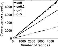
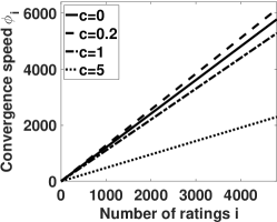
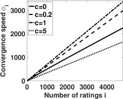
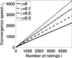
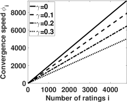
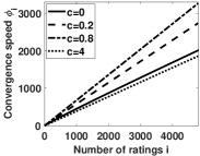
Impact of rating aggregation rules (). Recall that . Thus, we study the impact of rating aggregation rules through varying . Figure 2 shows the curve of across , where we vary from 0 to 5. Note that in the figure, we use to denote for brevity. From Figure 2, one can observe that the value of is almost linear in the number of ratings . This implies that the speed of convergence is roughly exponential in the number of ratings . Figure 2(a) shows that decreases in when . This implies that when there are no herding effects, the convergence speed of the simple unweighted average rule is faster than recency aware aggregation rules. However, when and , first increases and then decreases as we increase . This implies that in the presence of herding effects, recency aware aggregation rule can have faster speed of convergence. However, the strength of recency awareness should not be too strong. Furthermore, when and , the aggregation rules with and have the highest convergence speed respectively. Namely, as the strength of herding effects increases, the online rating system operator can increase the strength of recency awareness to speed up convergence.
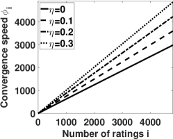
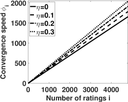
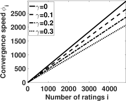
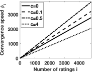
Impact of review selection mechanism (). Recall that each review selection mechanism is modeled via a parameter capturing the accuracy. Figure 3 shows as we vary from 0 to 0.3. One can observe that increases in . This shows that increasing the accuracy of review selection mechanism can speed up the convergence. The improvement of becomes small, as we increase . This implies that an accurate review selection mechanism can improve the convergence speed significantly only when the strength of recency awareness of an aggregation rule is not very strong.
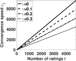
Impact of herding effects (). Recall that the herding effects is modeled via a parameter capturing the strength of herding. Figure 4 shows as we vary from 0 to 0.3. One can observe that decreases in . This shows that as users become more prone to herding effects, the speed of convergence slows down. The decrease of becomes small, as we increase . In other words, the rating aggregation rules having higher strength of recency awareness are more robust against herding effects.
Lessons learned. The recency aware aggregation rule can speed up the convergence over the simple unweighted average rule, but the strength of recency awareness should not be too strong. Increasing the the accuracy of a review selection mechanism can always improve the convergence speed, and this improvement decreases as the strength of recency awareness increases. Herding effects slow down the speed of convergence, but the aggregation rule with stronger strength of recency awareness can be more robust (in terms of convergence speed) against herding effects.
5.2. Evaluating the Inference Algorithm
Recall that and denote the inferred model parameters. We aim to study the accuracy of and in estimating the best linear approximation denoted by and . In general, the best linear approximation and is determined by the specific form of and . For simplicity, here we consider approximating a linear model, which is specified in Section 5.1, i.e., derived in Equation (2), and . Then the best linear approximation for this linear model is We define the relative estimation error as
| (6) |
We calculate and via the Monte Carlo simulation. For each round of simulation, we use our model (with parameters , , and , which will be specified later) to generate ratings. Inputting these ratings to our inference algorithm stated in Section 4.2, we obtain and for one round. Then, we compute one sample of and via Equation (6). We repeat this process for multiple rounds to obtain multiple samples of and . Lastly, we use the average of these samples to estimate and .
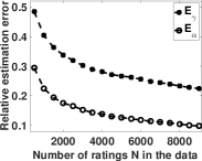
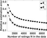
Figure 5 shows and across the number of ratings under both the honest rating and misbehaving rating scenarios, where we set , and We consider a large effective strength of herding effects , because the robustness of our inference algorithm (against misbehaving ratings) under small strength can be implied by this large strength. Figure 5(a) shows that under the honest rating scenario, both and decrease in the number of rating . This implies that the accuracy of our inference algorithm increases as more ratings are observed. Furthermore, the curve of lies above . This means that our inference algorithm has a higher accuracy in estimating the ground-truth collective opinion than the effective strength of herding effects . The error and can be as small as 10% and 20% respectively with thousands of ratings. Figure 5(b) presents and when we inject 50 misbehaving ratings (i.e., ) of 5. Compared to Figure 5(a), one can observe that our inference algorithm has similar accuracy as that of the honest rating case. This implies that our inference algorithm is robust against misbehaving ratings.
Lessons learned. Our inference algorithm can achieve a high accuracy under thousands of ratings and it is robust against misbehaving ratings.
6. Experiments on Real Data
We conduct experiments on real-world online ratings from Amazon and TripAdvisor. We identify recency aware rating aggregation rules, which improve the convergence speed in Amazon and TripAdvisor by 41% and 62% respectively.
6.1. Datasets and Parameter Inference.
We use the ratings of 32,888 products in Amazon and 11,543 hotels in TripAdvisor crawled in 2013. From the rating dataset we select the items (i.e., products in Amazon or hotels in TripAdvisor) with at least 2,000 ratings to attain a balance between inference accuracy and dataset scale. In total, 284 products in the Amazon dataset and 111 hotels in TripAdvisor dataset are selected. Note that Amazon and TripAdvisor use the simple unweighted average rule, i.e., . We apply the Algorithm stated in Section 4 to infer and for each selected item.

Figure 8 shows the cumulative distribution (CDF) of the inferred effective herding strength across items. One can observe that the cumulative distribution curve of Amazon lies above that of TripAdvisor roughly. The average of the inferred effective herding strengths for Amazon and TripAdvisor are and respectively. This implies that users in Tripadvisor are more likely to follow the crowd in providing ratings.
6.2. Rating Aggregation Rules and Implications
We consider . Figure 9 shows the value of as we vary from 0 to 4. Note that the Amazon and TripAdvisor practice , i.e., unweighted aggregation rule. One can observe that we can improve the speed of convergence in Amzaon by using a recency aware aggregation rule with and speed up the convergence in TripAdvisor by using a recency aware aggregation rule with . In other words, using these aggregation rules, we can reveal the ground-truth quality of products with the same accuracy by using significantly less ratings in both Amazon and TripAdvisor.

Lessons learned. We identify appropriate recency aware aggregation rules, which can improve the speed of convergence in Amazon and TripAdvisor by 41% and 62%.
7. Experiments on Real Data
We conduct experiments on real-world online ratings from Amazon and TripAdvisor. We identify recency aware rating aggregation rules, which improve the convergence speed in Amazon and TripAdvisor by 41% and 62% respectively.
7.1. Datasets and Parameter Inference.
We use the ratings of 32,888 products in Amazon and 11,543 hotels in TripAdvisor crawled in 2013. From the rating dataset we select the items (i.e., products in Amazon or hotels in TripAdvisor) with at least 2,000 ratings to attain a balance between inference accuracy and dataset scale. In total, 284 products in the Amazon dataset and 111 hotels in TripAdvisor dataset are selected. Note that Amazon and TripAdvisor use the simple unweighted average rule, i.e., . We apply the Algorithm stated in Section 4 to infer and for each selected item.
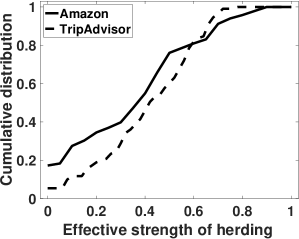
Figure 8 shows the cumulative distribution (CDF) of the inferred effective herding strength across items. One can observe that the cumulative distribution curve of Amazon lies above that of TripAdvisor roughly. The average of the inferred effective herding strengths for Amazon and TripAdvisor are and respectively. This implies that users in Tripadvisor are more likely to follow the crowd in providing ratings.
7.2. Rating Aggregation Rules and Implications
We consider . Figure 9 shows the value of as we vary from 0 to 4. Note that the Amazon and TripAdvisor practice , i.e., unweighted aggregation rule. One can observe that we can improve the speed of convergence in Amzaon by using a recency aware aggregation rule with and speed up the convergence in TripAdvisor by using a recency aware aggregation rule with . In other words, using these aggregation rules, we can reveal the ground-truth quality of products with the same accuracy by using significantly less ratings in both Amazon and TripAdvisor.

Lessons learned. We identify appropriate recency aware aggregation rules, which can improve the speed of convergence in Amazon and TripAdvisor by 41% and 62%.
8. Application: Rating Prediction
To demonstrate the versatility of our model, we parametrize our model to predict subsequent ratings. We apply regularized least square to infer model parameters. Extensive experiments on four datasets demonstrate that our model can improve the accuracy of Herd and the HIALF .
8.1. Applying Our Models to Rating Prediction
We consider the following rating prediction problem: given a set of historical ratings of items, predict subsequent ratings of items. To apply our model to address this problem, we next first parameterize our model and then infer model parameters.
Let denote the ubiased rating of user toward . Namely, characterizes user ’s intrinsic overall opinion toward item
Modeling initial opinion formation. Now we model the initial opinion formation, i.e., the function . Users may form initial opinions from the aggregation of historical ratings or a small number of latest ratings. We first consider the case that users form initial opinions from the aggregation of historical ratings. Denote the collective opinion summarized from the rating history as
where and . The is public to all users. We consider a class of weighted aggregation rules to summarize historical ratings:
| (7) |
where denotes the weight associated with -th rating, and is an indicator function. For example, , is deployed in Amazon and TripAdvisor, which corresponds to “average rating rule”. Under this average rating rule, we have , which is the fraction of historical ratings equal . Note that is displayed to all users. We capture the aggregate opinion heterogeneity in initial opinion formation as follows:
| (8) |
where the weight models how a user weighs the opinion associated with each rating level. For example, a user may assign a large weight to low ratings representing that she is sensitive to negative opinions. There are several possible parametric forms of the weights:
where .
Now, we consider the case that users form initial opinions from a small number of latest ratings. Let denote the number of latest ratings that users refer to for initial opinion formation. We capture rating recency in initial opinion formation as:
| (9) |
where the weight satisfies and we set for all by default. There are several possible forms of the weight . One can use the following forms of to model arrival order aware initial opinion formation:
where . One can use the following forms of to model arrival time stamp aware initial opinion formation:
where denotes the arrival time of user , , we set by default for all .
Model parameterization. The Herd algorithm was proposed by Wang et al. , which is the first algorithm exploring Herd effects to improve rating prediction. We will use Herd as a major comparison baseline. For fair comparison with Herd , we parameterize via the classical latent factor (LF) model :
| (10) |
In Equation (10), and represent vectors of latent features for user and product , where . The and model user and product bias respectively. The models the constant shift or residual. All parameters in Equation (10) are unknown and will be inferred from the data. Similarily, we parametrize the strength of herding effects as:
where is unknown parameters to be inferred from data. Note this parametrization method was used in , and we choose it for fair comparison with Herd. We will show that our model can outperform all the baselines. This implies that if one selects them with finer tuning, our model can achieve better performance. We summarize all parameters to be inferred from data as
All the hyper parameters will be given before model training.
Model inference. Consider a training rating dataset, in which product has historical ratings. We aim to infer from the training rating dataset. In particular, we use regularized least square method to infer :
We use stochastic gradient descent (SGD) algorithm to learn model parameters . Note that SGD was widely used in previous works to improve training efficiency
Rating prediction. Let denote the inferred model parameter set. To illustrate, suppose we are going to predict the -th rating of item , i.e., . Note that is the user who assign the rating . We are given the ID of the user denoted by . Then we predict the rating as , which are computed using our model with the inferred parameters . We denote our rating prediction method as R-HE.
8.2. Evaluation Settings
The dataset. We use four public datasets to evaluate the accuracy of our AC-RP method, whose overall statistics are summarized in Table 1. The dataset from Amazon was published in and it contains historical ratings of movies in Amazon. The dataset from Google Local was published in and it contains reviews about businesses from Google Local (Google Maps). The dataset from TripAdvisor was published in , and it contains historical ratings of hotels in TripAdvisor. The dataset from Yelp was downloaded from the link 222https://www.yelp.com/dataset and it contains historical ratings for restaurants in Yelp.
| category | # products | # users | # ratings |
|---|---|---|---|
| Amazon-movie | 208,321 | 2,088,620 | 4,607,047 |
| Googlelocal | 4,567,431 | 3,116,785 | 10,601,852 |
| TripAdvisor | 1,705 | 623,567 | 871,689 |
| Yelp | 60,785 | 366,715 | 1,569,264 |
For fair comparison with Herd, we use the same method as HIALF (Zhang2019, ) to extract training dataset and testing dataset. Similar with HIALF , for each item in Table 1, we only select items with an medium positive average rating, i.e., average rating in the range out. For each selected item we extract all its ratings and the associated users out. We then remove items with less than 50 training ratings, to avoid over-fitting. Table 2 summarizes overall statistics of the selected data. One can observe that after this selection, some datasets still contain around two hundred thousands of users. Comparing the number of ratings with the number of users, one can observe that the rating matrix is very sparse. Similar with HIALF , we further aggregate users with twenty ratings (or fifty) as a big user for Googlelocal and TripAdvisor ( or Amazon-movie and Yelp). Furthermore, for each selected item, we use its last 25 ratings as test ratings and use all other ratings as training ratings. We train the models on the training dataset, and validate the model on the testing dataset.
| category | # products | # users | # ratings |
|---|---|---|---|
| Amazon-movie | 1,118 | 198,209 | 271,295 |
| Googlelocal | 445 | 38,553 | 53,740 |
| TripAdvisor | 309 | 134,484 | 150,201 |
| Yelp | 736 | 82,509 | 157,463 |
Comparison baseline & metrics. We use the root mean squared error (RMSE) to quantify the testing accuracy:
| (11) |
where denotes an estimation of , which is computed using our model with the inferred parameters . We compare our AC-RP method with the following three baselines.
-
•
HIALF . The HIALF algorithm was proposed by Zhang et al. , which is the first algorithm exploring assimilate-contrast effects to improve rating prediction.
-
•
Herd . The Herd algorithm was proposed by Zhang et al., which explores herding effects to improve rating prediction.
Parameter setting. To prevent over fitting, we set appropriate regularization hyper parameters for our models. Following similar principle in HIALF , we consider the regularization hyper parameters summarized in Table 3. Following previous work , we choose the dimension of latent features as . For the other hyper parameters, we will select them systematically and present them with the experiment results.
| 0.1 | 0.01 | 5 |
8.3. Rating Recency for Rating Prediction
In this section, we evaluate the benefit of exploiting rating recency for rating prediction tasks. Consider that under rating recency, users form initial opinion from latest ratings. We consider the initial opinion formation model derived in Equation
Impact of . The initial opinion is the simple average of latest ratings, i.e., . Table 4 shows the RMSE of Herd, HIALF and our B-HE method. In Table 4, the column corresponds to the RMSE of our B-HE method with . One can observe that when , our method has a smaller RMSE than Herd. This statement also holds when . Namely, under some simple selections of , our method has a higher rating prediction accuracy than Herd. Note that this improvement of rating prediction accuracy by exploiting rating recency is supported by survey studies, which identified that users tend to read a small number of latest reviews or ratings to form initial opinions . The RMSE of our method varies as we increase from 20 to 80, This implies that is an important factor for the rating prediction accuracy and one needs to exploit the rating recency carefully for rating prediction. The above improvement on the rating prediction accuracy is achieved at simple selections of . One may further improve the rating prediction accuracy by finer tuning of . In this experiment, the initial opinion is the simple average of latest ratings. Users may have different weights to different ratings, i.e., more weights on more recent ratings. In the following, we explore this direction.
| category | Herd | HIALF | RobustAVG |
|---|---|---|---|
| Amazon-movie | 1.4871 | 1.2209 | 1.1848 |
| Googlelocal | 1.1412 | 1.0616 | 1.1013 |
| TripAdvisor | 1.1838 | 0.9208 | 1.1307 |
| Yelp | 1.4200 | 1.2006 | 1.0059 |
| category | =20 | =40 | =80 |
| Amazon-movie | 1.1827 | 1.1842 | 1.1847 |
| Googlelocal | 1.0995 | 1.1007 | 1.1013 |
| TripAdvisor | 1.1299 | 1.1301 | 1.1305 |
| Yelp | 1.0037 | 1.0050 | 1.0058 |
Impact of arrival order. The are two types of weights on ratings, i.e., based on arrival order and based on arrival time stamp of ratings. Here we study the weight which is based on arrival order. We fix . To study the impact of arrival order, we consider three types of weights associated with the arrival order of ratings, i.e., exponential, polynomial and logarithmic in the arrival order, which are stated in Table 5. Table 5 shows that RMSE of our R-BE method under these three types of weights. Consider that the weight is exponential in the arrival order, i.e., . One can observe that as we vary the parameter of from 0.01 to 0.0001, the RMSE can be further reduced over the unweighted case, i.e., . Similar observations can be found when the weight is polynomial or logarithmic in the arrival order of ratings. This implies that one can further improve the rating prediction accuracy via tuning the weight of ratings based on the arrival order. This improvement on rating prediction accuracy is supported by that users tend to assign larger weights to more recent ratings Furthermore, this improvement is achieved at simple selections of the weight of ratings. One can further improve the rating prediction accuracy by finer tuning of weights.
| category | Herd | =0.01 | =0.001 | =0.0001 | |
|---|---|---|---|---|---|
| Amazon-movie | 1.4871 | 1.1823 | 1.1824 | 1.1824 | |
| Googlelocal | 1.1412 | 1.0999 | 1.0999 | 1.0999 | |
| TripAdvisor | 1.1838 | 1.1300 | 1.1320 | 1.1311 | |
| Yelp | 1.4200 | 1.0033 | 1.0033 | 1.0033 | |
| —— | |||||
| =0.5 | =1 | =2 | =0.5 | =1 | =2 |
| 1.1817 | 1.1818 | 1.1818 | 1.1817 | 1.1814 | 1.1831 |
| 1.0993 | 1.0993 | 1.0993 | 1.0993 | 1.1001 | 1.1026 |
| 1.1299 | 1.1299 | 1.1299 | 1.1299 | 1.1303 | 1.1287 |
| 1.0028 | 1.0028 | 1.0028 | 1.0028 | 1.0043 | 1.0038 |
Impact of arrival time stamp. We fix . To study the impact of arrival time stamp, we consider three types of weights associated with the arrival time stamp of ratings, i.e., exponential, polynomial and logarithmic in the arrival time stamp, which are stated in Table 6. Table 6 shows that RMSE of our R-BE method under these three types of weights. Consider that the weight is exponential in the arrival time stamp, i.e., . One can observe that as we vary the parameter of from 0.01 to 0.0001, the RMSE can be further reduced over the unweighted case, i.e., . Similar observations can be found when the weight is polynomial or logarithmic in the arrival time stamp of ratings. This implies that one can further improve the rating prediction accuracy via tuning the weight of ratings based on the arrival time stamp. This improvement on rating prediction accuracy is supported by that users tend to assign larger weights to more recent ratings (Rudolph2015, ). Furthermore, this improvement is achieved at simple selections of the weight of ratings. It can be further improved by finer tuning of weights.
| category Herd | =0.01 | =0.001 | =0.0001 | ||
|---|---|---|---|---|---|
| Amazon-movie | 1.4871 | 1.1823 | 1.1823 | 1.1823 | |
| Googlelocal | 1.1412 | 1.0998 | 1.0999 | 1.0999 | |
| TripAdvisor | 1.1838 | 1.1300 | 1.1300 | 1.1300 | |
| Yelp | 1.4200 | 1.0037 | 1.0037 | 1.0037 | |
| —— | |||||
| =0.2 | =0.4 | =0.8 | =0.2 | =0.4 | =0.8 |
| 1.1623 | 1.1623 | 1.1623 | 1.1623 | 1.1623 | 1.1623 |
| 1.0991 | 1.0991 | 1.0999 | 1.0992 | 1.00989 | 1.0999 |
| 1.1299 | 1.1299 | 1.1303 | 1.1320 | 1.1320 | 1.1320 |
| 1.0031 | 1.0031 | 1.0049 | 1.0031 | 1.0030 | 1.0045 |
8.4. Aggregate Opinion Heterogeneity for Rating Prediction
In this section, we study the benefit of exploiting aggregate opinion heterogeneity for rating prediction. We consider the initial opinion formation model derived in Equation (8). Table 7 shows the RMSE of our R-BE method under the case that the weight is exponential in opinion levels. In Table 7, we only compare our R-BE method with Herd. One can observe that as we vary the parameter of from 0.01 to 0.0001, the RMSE can be further reduced over Herd. Similar observations can be found when the weights is polynomial or logarithmic in rating level as shown in Table 8 and 9. This implies that one can further improve the rating prediction accuracy via tuning the weight of rating levels, i.e., aggregate opinion heterogeneity. This improvement on rating prediction accuracy is supported by that users tend to assign different weights to different rating levels (Rudolph2015, ) This reduction of RMSE is achieved at simple selections on weight for rating levels. Finer tuning of weight may lead to further reduction on the RMSE.
| category | Herd | =0.1 | =0.01 | =0.001 |
|---|---|---|---|---|
| Amazon-movie | 1.4871 | 1.1661 | 1.1824 | 1.1844 |
| Googlelocal | 1.1412 | 1.1155 | 1.1026 | 1.1016 |
| TripAdvisor | 1.1838 | 1.1387 | 1.1312 | 1.1308 |
| Yelp | 1.4200 | 0.9929 | 1.0043 | 1.0057 |
| category | Herd | =-0.1 | =-0.01 | =-0.001 |
| Amazon-movie | 1.4871 | 1.2115 | 1.1871 | 1.1851 |
| Googlelocal | 1.1412 | 1.0923 | 1.1002 | 1.1018 |
| TripAdvisor | 1.1838 | 1.1292 | 1.1303 | 1.1307 |
| Yelp | 1.4200 | 1.0230 | 1.0074 | 1.0062 |
| category | Herd | =0.5 | =1 | =2 |
|---|---|---|---|---|
| Amazon-movie | 1.4871 | 1.1618 | 1.1613 | 1.1615 |
| Googlelocal | 1.1412 | 1.1203 | 1.1449 | 1.1436 |
| TripAdvisor | 1.1838 | 1.1437 | 1.1690 | 1.1463 |
| Yelp | 1.4200 | 0.9896 | 0.9846 | 0.9833 |
| category | Herd | =-0.5 | =-1 | =-2 |
| Amazon-movie | 1.4871 | 1.2149 | 1.2388 | 1.2621 |
| Googlelocal | 1.1412 | 1.0926 | 1.0889 | 1.0868 |
| TripAdvisor | 1.1838 | 1.1293 | 1.1310 | 1.1340 |
| Yelp | 1.4200 | 1.0229 | 1.0359 | 1.0498 |
| category | Herd | =0.5 | =1 | =2 |
|---|---|---|---|---|
| Amazon-movie | 1.4871 | 1.1608 | 1.1607 | 1.1619 |
| Googlelocal | 1.1412 | 1.1261 | 1.1480 | 1.1376 |
| TripAdvisor | 1.1838 | 1.1495 | 1.1705 | 1.1482 |
| Yelp | 1.4200 | 0.9871 | 0.9839 | 0.9846 |
| category | Herd | =-0.5 | =-1 | =-2 |
| Amazon-movie | 1.4871 | 1.2331 | 1.2729 | 1.2842 |
| Googlelocal | 1.1412 | 1.0893 | 1.0858 | 1.0876 |
| TripAdvisor | 1.1838 | 1.1305 | 1.1370 | 1.1474 |
| Yelp | 1.4200 | 1.0336 | 1.0620 | 1.0941 |
9. Related Work
Online product rating (or review) systems has been studied extensively. A number of works investigated whether and how online product rating systems can benefit sellers and users. Chevalier et al. (Chevalier2006, ) studied the impact of product reviews on the sales of sellers, and they found that positive product reviews can increase the sales. Mudambi et al. (Mudambi2010, ) studied the impact of product reviews on customer’s purchasing behavior, and found that product reviews are helpful in purchasing decision makings. Similar observations were found by Lackermair et al. (Lackermair2013, ) and Li (Li2013, ). We refer readers to (BrightLocal2016, ; Rudolph2015, ; Shrestha2016, ) for a number of survey studies on the role of product reviews in purchasing decisions.
A variety of works investigated rating (or review) biases. A number of sources that can lead to rating biases has been revealed, e.g., product categories (Guo2015, ), system interfaces (Cosley2003, ), recommendation algorithms (Shafto2016, ), the dynamics of user preferences (Koren2009, ), the improvement of user expertise (McAuley2013, ), etc. To mitigate these biases, a number of methods or algorithms were developed, e.g., (Cosley2003, ; Guo2015, ; Koren2009, ; McAuley2013, ; Shafto2016, ). Our work is closed related to the studied of rating bias from psychological perspectives. Zhang et al. (Zhang2017, ) modeled the assimilate and contrast phenomenon in ratings, and they used the model to improve recommendation accuracy. The herding effects in product ratings were revealed by a number of real-workd experiments (Salganik2006, ; Muchnik2013, ). Krishnan et al. (Krishnan2014, ) and Wang et al. (Wang2014, ) developed models to quantify the effect of herding effects (or social influence biases). Coba et al. (Coba2018, ) did some experiments to study how rating summaries influence user decisions. These works provided evidences for the existence of herding effects in online product rating systems. Built on these evidences, we investigate the convergence of product ratings. We also demonstrate how to utilize these convergence properties to manage product ratings.
10. Conclusion
We develop a framework to manage online product ratings. We formulate a mathematical model to characterize the herding effects, and the decision space to correct product ratings. We identify a class of rating aggregation rules, under which the historical collective opinion converges to the ground-truth collective opinion. We derive a metric to quantify the speed of convergence, which also guides product rating managing. Via theoretical analysis and experiment studies we found: (1) recency aware aggregation rules can significantly speed up the convergence over the unweighted average rule (commonly deployed) especially under strong herding effects; (2) the convergence speed increases in the accuracy of the review selection mechanism but this improvement becomes small when the aggregation rule has a strong recency awareness; (3) recency aware rating aggregation rules can improve the convergence speed in Amazon and TripAdvisor by 41% and 62% respectively.
References
- (1) G. Lackermair, D. Kailer, and K. Kanmaz, “Importance of online product reviews from a consumer’s perspective,” Advances in Economics and Business, vol. 1, no. 1, pp. 1–5, 2013.
- (2) M. Li, L. Huang, C.-H. Tan, and K.-K. Wei, “Helpfulness of online product reviews as seen by consumers: Source and content features,” International Journal of Electronic Commerce, vol. 17, no. 4, pp. 101–136, 2013.
- (3) Y. Zhao, S. Yang, V. Narayan, and Y. Zhao, “Modeling consumer learning from online product reviews,” Marketing Science, vol. 32, no. 1, pp. 153–169, 2013.
- (4) J. Berger, Bad Reviews Can Boost Sales. Here’s Why. Harvard Business Review, 2012.
- (5) M. Luca, “Reviews, reputation, and revenue: The case of yelp. com,” 2016.
- (6) S. Zaroban, Product reviews boost revenue per online visit 62%. Digital Commerce, 2015.
- (7) L. Muchnik, S. Aral, and S. J. Taylor, “Social influence bias: A randomized experiment,” Science, vol. 341, no. 6146, pp. 647–651, 2013.
- (8) M. J. Salganik, P. S. Dodds, and D. J. Watts, “Experimental study of inequality and unpredictability in an artificial cultural market,” science, vol. 311, no. 5762, pp. 854–856, 2006.
- (9) H. Xie and J. C. S. Lui, “Mathematical modeling and analysis of product rating with partial information,” ACM Trans. Knowl. Discov. Data, vol. 9, no. 4, pp. 26:1–26:33, 2015.
- (10) BrightLocal, Local Consumer Review Survey. BrightLocal, 2016.
- (11) K. Shrestha, 50 Stats You Need to Know About Online Reviews [Infographic]. Vendasta, 2016.
-
(12)
SupplementaryFile, Robust Product Rating Rules Against Herding Effects:
Theory and Applications.
https://1drv.ms/b/s!AkqQNKuLPUbEii73M4esYvRveTyj?e=ilSYyw, 2020. - (13) N. Jindal and B. Liu, “Review spam detection,” in Proc. of WWW, 2007.
- (14) X. Zhang, H. Xie, J. Zhao, and J. C. Lui, “Understanding assimilation-contrast effects in online rating systems: modelling, debiasing, and applications,” ACM Transactions on Information Systems (TOIS), vol. 38, no. 1, pp. 1–25, 2019.
- (15) S. Rudolph, 50 Stats You Need to Know About Online Reviews [Infographic]. Business 2 Community, 2016.
- (16) J. A. Chevalier and D. Mayzlin, “The effect of word of mouth on sales: Online book reviews,” Journal of marketing research, vol. 43, no. 3, pp. 345–354, 2006.
- (17) S. M. Mudambi and D. Schuff, “What makes a helpful online review? a study of customer reviews on amazon.com,” MIS Quarterly, vol. 34, no. 1, pp. 185–200, 2010.
- (18) F. Guo and D. B. Dunson, “Uncovering systematic bias in ratings across categories: A bayesian approach,” in Proc. of ACM RecSys, 2015.
- (19) D. Cosley, S. K. Lam, I. Albert, J. A. Konstan, and J. Riedl, “Is seeing believing? how recommender system interfaces affect users’ opinions,” in Proceedings of the SIGCHI conference on Human factors in computing systems, 2003, pp. 585–592.
- (20) P. Shafto and O. Nasraoui, “Human-recommender systems: From benchmark data to benchmark cognitive models,” in Proc. of ACM RecSys, 2016.
- (21) Y. Koren, “Collaborative filtering with temporal dynamics,” in Proc. of ACM KDD, 2009.
- (22) J. J. McAuley and J. Leskovec, “From amateurs to connoisseurs: modeling the evolution of user expertise through online reviews,” in Proceedings of the 22nd international conference on World Wide Web, 2013, pp. 897–908.
- (23) X. Zhang, J. Zhao, and J. C. S. Lui, “Modeling the assimilation-contrast effects in online product rating systems: Debiasing and recommendations,” in Proc. of ACM RecSys, 2017.
- (24) S. Krishnan, J. Patel, M. J. Franklin, and K. Goldberg, “A methodology for learning, analyzing, and mitigating social influence bias in recommender systems,” in Proc. of ACM RecSys, 2014.
- (25) T. Wang, D. Wang, and F. Wang, “Quantifying herding effects in crowd wisdom,” in Proc. of ACM KDD, 2014.
- (26) L. Coba, M. Zanker, L. Rook, and P. Symeonidis, “Exploring users’ perception of rating summary statistics,” in Proceedings of the 26th Conference on User Modeling, Adaptation and Personalization. ACM, 2018, pp. 353–354.
Appendix A Technical Proofs
Proof of Lemma 1:
First we have
Then if follows that
Therefore,
is decreasing in .
Proof of Theorem 1: Let denote an dimensional vector, whose -th entry is 1, i.e., and all the other entries are zero, i.e., and . Note that equals to . Then we have that
This implies a useful equation for later proof Then we can derive as follows:
where we define as Let denote a mapping defined as Then it follows that is a pseudo-contraction mapping
Note that we conclude the pseudo-contraction mapping, because . Then it follows that has a unique fixed point . One can also check that the error vector satisfies
Furthermore,
Lastly, note that satisfies
Then it follows that
converges to the unique fixed point of almost surely.
Then it follows that
Proof of Theorem 2:
Note that the number of misbehaving ratings is finite
and the index of the last misbehaving rating is .
Let us now consider for all
.
Note that from the proof of Theorem 1,
one can observe that the convergence of
is invariant of the initial historical collective opinion,
i.e., .
Therefore the sequence of historical collective opinion
still converges to almost surely.
Proof of Theorem 3: Without loss of generality, let us consider one entry of the historical collective opinion , i.e., . From the proof of Theorem 1, we have that Then it follows that
Let . Then we can further have
Note that and define . For the simplicity of presentation, let us define Then it follows that
Note that Thus forms a martingale with respect to . To study the convergence rate of , let us first check the difference between and .
For simplicity of presentation, we define
where . Then it follows that Furthermore, we we have Note that . This implies that . Then we have . Then applying the martingale concentration theory (in particular the Azuma Hoeffiding inequality) we have
This proof is then complete.
Proof of Theorem 4: First we can rewrite as
Note that we can further have
Observe that the term
.
Thus the term
is non-decreasing in
and is non-increasing in .
Therefore,
is non-decreasing in
and is non-increasing in
for all .
We can then conclude this theorem.
Proof of Theorem 5: Note that the number of misbehaving ratings is finite and the index of the last misbehaving rating is . Let us now consider for all . Let . Then it follows that Now we treat as the starting point. Note that the sequence forms a martingale, i.e., for all . Furthermore, the difference still holds and satisfies Note that for all . Then it follows that
Then by some algebraic operations, we have
This proof is then complete.
Proof of Theorem 6: Consider the average score rule. Note that implies By the union bound, we have
Namely, with probability at least we have that holds for all . Then with probability at least , it holds that
Now, let us consider the majority rule. With a similar proof, one can conclude that with probability at least , it holds that for all . Then we have that
Consider , we have
Namely, the true quality is still revealed.