ViLReF: A Chinese Vision-Language
Retinal Foundation Model

Abstract

Subtle semantic differences in retinal image and text data present great challenges for pre-training visual-language models. Moreover, false negative samples, i.e., image-text pairs having the same semantics but incorrectly regarded as negatives, disrupt the visual-language pre-training process and affect the model’s learning ability. This work aims to develop a retinal foundation model, called ViLReF, by pre-training on a paired dataset comprising 451,956 retinal images and corresponding diagnostic text reports. In our vision-language pre-training strategy, we leverage expert knowledge to facilitate the extraction of labels and propose a novel constraint, the Weighted Similarity Coupling Loss, to adjust the speed of pushing sample pairs further apart dynamically within the feature space. Furthermore, we employ a batch expansion module with dynamic memory queues, maintained by momentum encoders, to supply extra samples and compensate for the vacancies caused by eliminating false negatives. Extensive experiments are conducted on multiple datasets for downstream classification and segmentation tasks. The experimental results demonstrate the powerful zero-shot and transfer learning capabilities of ViLReF, verifying the effectiveness of our pre-training strategy. Our ViLReF model is available at: https://github.com/T6Yang/ViLReF.

I Introduction

Foundation models pre-trained on large datasets are receiving increasing attention in computer vision and natural language processing due to their impressive generalization capabilities when fine-tuned on various downstream tasks [1, 2]. With the availability of training data of ophthalmology, retinal foundation models have recently gained much attraction and are widely employed in clinical applications. Retinal images and their corresponding diagnostic reports, the two common and enormous data modalities have been proposed for training retinal foundation models. Compared with natural images, differences among retinal images are often more subtle [3]. The main structures are very similar in both normal and diseased retinal images, with few tiny areas showcasing pathological differences, which brings a great challenge to construct retinal foundation models based on self-supervised contrastive learning.

Figure 1: Overview of the proposed vision-language pre-training strategy. Labels are extracted from Chinese retinal diagnostic reports to provide extra supervision for image-text contrastive learning, mitigating the effect caused by false negative samples. Note: The text in the gray box is the English translation of the adjacent Chinese text.

Self-supervised contrastive vision-language joint representation learning is a common strategy to train foundation models, which typically does not require additional manual annotations except for the diagnostic reports [4]. Theoretically, this strategy possesses the ability to learn semantic representations of an unlimited variety of lesions and diseases [5]. However, traditional self-supervised contrastive learning strategies may treat image-text pairs having the same semantics as negative samples (i.e., false negative samples) and push them apart during pre-training, which introduces noise, obscure the appearance of pathological differences to models, and lead to confusion in learning clinically relevant visual representations. One way to mitigate the effect caused by false negative samples is to introduce extra supervision during pre-training.

According to the text reports, a series of labels can be extracted automatically to provide supervision and avoid the occurrence of false negatives. The Unified Medical Language System (UMLS) [6] recognizes clinically defined entities within text reports to extract labels conveniently [7]. However, there is no Chinese UMLS available, and existing methods for identifying Chinese entities using UMLS predominantly rely on translation and mapping. The quality of translation affects the results of mapping significantly, thereby limiting the efficiency and effectiveness of mapping algorithms [8]. Moreover, some entities cannot be converted into labels after being identified directly, thus they require further logical decisions based on expert knowledge. Therefore, to accommodate large and diverse retinal diagnostic reports in Chinese and ensure accurate and effective label generation, a new method to acquire supervision labels from Chinese retinal text reports is needed.

To this end, we present an expert-knowledge-based report converter for data pre-processing to convert Chinese text reports into supervision labels, and propose a novel pre-training strategy for retinal foundation models, as illustrated in Fig. 1. A novel constraint in the feature space, leveraging the labels, is proposed to adjust the speed of pushing sample pairs apart dynamically, mitigating the effect caused by false negative samples during pre-training. When the sample pairs have the same labels, they are eliminated during contrastive learning. This brings a new challenge: the number of contrastive samples might be reduced, affecting the pre-training process.

To compensate for the weakened contrastive learning effect resulting from the elimination of false negatives, memory queues are maintained by momentum encoders to expand the quantity of contrastive samples. Ultimately, we propose ViLReF, a Chinese Vision-Language Retinal Foundation model, which comprises two aligned universal retinal image and text feature extractors. The main contributions of this work can be summarized as follows:

• We propose ViLReF, a foundation model pre-trained on a dataset of 451,956 paired retinal images and corresponding diagnostic reports provided by Beijing Tongren Hospital. Utilizing contrastive learning without reliance on pretext tasks during pre-training, ViLReF effectively understands and aligns rich visual and language semantic representations of ophthalmic data. Our vision-language pre-training strategy helps the model capture subtle but clinically significant visual patterns in the data.

• To address the challenge of false negative samples while ensuring effective representation learning during pre-training, we introduce a novel contrastive learning pre-training strategy. Specifically, we develop the expert-knowledge-based report converter, which leverages domain knowledge to extract labels from Chinese retinal diagnostic text reports. Additionally, we propose the Weighted Similarity Coupling Loss to optimize the coupling distribution of feature and label similarities, aiding the model in learning robust representations. Furthermore, we employ a batch expansion module with dynamic memory queues to compensate for the absent contrastive samples caused by the elimination of false negatives.

• We extensively evaluate ViLReF’s zero-shot and fine-tuned inference performance on various downstream tasks across multiple datasets. Compared with existing pre-training strategies, our method demonstrates impressive effectiveness, endowing ViLReF with excellent semantic understanding and generalization capabilities in the ophthalmic domain.

II Related Work

II-A Vision-language Pre-trained Foundation Models

Pre-training is the basis of foundation models, aiming to enable the model to learn representations of data. Compared with training models from scratch, pre-training improves the robustness of the model and endows better generalization capabilities. Unsupervised pre-training can be regarded as a regularization that places the starting point of optimization on a data-dependent manifold [9].

The pre-training strategies of foundation models can be generally divided into two categories: learning from auxiliary pretext tasks and contrastive learning. Auxiliary pretext tasks are typically achieved through self-supervision. These tasks generate pseudo labels and help the model extract representative knowledge from the data [10]. For example, InsLoc [11] builds a target detection pretext task by clipping and synthesizing images to learn representations of the target data. Frameworks dedicated to super-resolution, such as HIPA [12] and NasmamSR [13], are also commonly employed for representation extraction and understanding. In retinal domain, foundation models like RETFound [14] and EyeFound [15] incorporate the principles of masked autoencoders (MAE) [16]. These models learn information-dense image representations by predicting masked regions of input data, demonstrating state-of-the-art performance in critical tasks such as disease prediction, diagnosis, and prognosis.

Contrastive learning offers a straightforward method for learning representations by pulling features of positive samples closer and pushing features of negative samples further apart. Sample pairs are selected during pre-training dynamically [17]. For example, SimCLR [18] promotes alignment between different augmented views of an image through a learnable non-linear projection and a contrastive loss function. To address the sensitivity of InfoCE loss to batch size, MoCo [19] uses output representations of a momentum-updated encoder’s as the embedding repository rather than those from the trained network. DINO [20] enhances the representative consistency across rescaled image crops using self-supervised distillation. SwAV [21] and PCL [22] first cluster the data to avoid computationally intensive pairwise comparisons and reduce false negative pairs during contrastive learning.

Contrastive pre-training strategies, exemplified by CLIP [2], which combines vision and language to match positive and negative sample pairs automatically, are growing in popularity. Among medical data sources, images and their associated text descriptions are two common and abundant data modalities. The emergence of large-scale medical datasets such as MIMIC-CXR [23], PadChest [24] and ROCO [25], provides necessary data to pre-train foundation models within medical domain.

In recent years, various studies have explored contrastive pre-trained vision-language foundation models in medical domain. ConVirt [26] processes image patches and sentence snippets into different but semantically aligned views to learn cross-modal representations bidirectionally. BioMedCLIP [27] utilizes 15 million image-text pairs extracted from biomedical and life science literature for pre-training, achieving top performance on various downstream tasks. GLoRIA [4] applies global loss and sub-region loss to extract representations at multiple scales, capturing semantic information of different granularities within the data. In retinal domain, RetiZero[28] leverages 341,896 retinal image-text pairs sourced from public datasets, ophthalmic literature, and online resources, covering over 400 retinal diseases. To reflect real-world clinical scenarios, RET-CLIP [29] utilizes binocular image-text datasets to learn representations at the levels of left eye, right eye, and patient as a whole.

II-B Expert Knowledge as Additional Supervision

Compared with the natural domain, data in medical domain exhibits finer-grained, denser, and more specialized semantics. In ophthalmological diagnosis through retinal images, interpretative descriptions characterize structural appearances (e.g., optic disk color, blood vessel orientation, retinal nerve fiber thickness) and local lesions (e.g., exudation, retinopathy patterns, neovascularization). Diagnostic reports serve as the clinical decision presented to healthcare facilities and patients, indicating the presence or absence of conditions like arteriosclerosis, diabetic retinopathy (DR), and glaucoma. While interpretive and diagnostic contents are presented at different levels, they are highly interdependent and predominantly associated with expert knowledge.

Medical tasks driven by expert knowledge typically follow agent-based paradigms. For instance, comprehensive observation of exudation, hemorrhaging, neovascularization, and retinal damage can indicate DR [30]. Drusen size and retinal pigment epithelium changes are correlated to age-related retinopathy staging [31]. Expert knowledge also serves as clinical priors. For example, the segmentation results of exudates in retinal images can be used to judge the severity of macular edema [32], and the diameter ratio of optic cup (OC) and optic disk (OD) can be used to determine the presence of glaucoma [33].

Contrastive learning foundation models pre-trained on image and text data, such as CLIP, often fail to fully capitalize on the expert knowledge contained in medical data, risking the loss of fine-grained representations during the pre-training process. Additionally, false negative sample pairs can reduce the model performance significantly. To address these challenges, existing strategies have leveraged expert knowledge to obtain additional supervision and apply it to the contrastive learning. For example, MedCLIP [3] uses rule-based label extraction from clinical texts and decouples image-text associations, vastly increasing the data available for pre-training while alleviating the false negative confusion. MedKLIP [34] enhances representation learning by incorporating clinical expert knowledge and disease descriptions. In retinal domain, FLAIR [35] uses a pre-training dataset built from 37 open-source datasets with category labels and maps these labels into text descriptions using expert knowledge, addressing the scarcity of text-based supervision in public retinal datasets. KeepFIT[36] leverages high-quality image-text pairs collected from professional fundus diagram books. It employs image similarity-guided text revision and a mixed pre-training strategy to infuse expert knowledge.

In contrastive representation learning within retinal domain, we leverage expert knowledge to extract diagnostic labels from detailed clinical medical data as additional supervision, thereby mitigating the effect of false negatives and enabling the model to understand finer-grained pathological structures and learn accurate clinical reasoning.

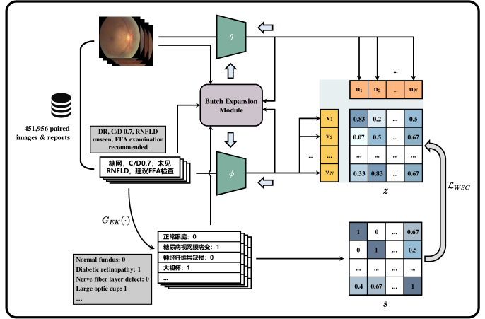
(a)

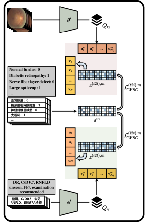
(b)

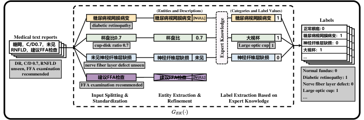
(c)

(d)

Figure 2: Flowchart of our vision-language pre-training strategy. (a) The backbone of the ViLReF model pre-training. (b) Illustration of the batch expansion module. (c) Illustration of the expert knowledge-based report converter. (d) Legend of symbols presented in the flowchart. Note: The text in the gray box is the English translation of the adjacent Chinese text.

III Method

In this section, we introduce the pre-training process and technical details of our model. The workflow is illustrated in Fig. 2a. After sampling a batch of retinal image-text pairs from the dataset, we first extract labels from the text report using the proposed expert-knowledge-based report converter $G_{EK}(\cdot)$. Features are then extracted by the image encoder $\theta(\cdot)$ and the text encoder $\phi(\cdot)$. We use the proposed Weighted Similarity Coupling Loss $\mathcal{L}_{WSC}$ to constrain the feature similarities of images and texts based on the prior similarities between their labels. Meanwhile, we employ a batch expansion module with dynamic memory queues, maintained by the momentum encoders $\theta^{\prime}(\cdot)$ and $\phi^{\prime}(\cdot)$, to effectively expand the equivalent batch size.

III-A Label Extraction Driven by Expert Knowledge

The extraction of labels for additional supervision, guided by rules built on expert knowledge, is a pre-processing step before pre-training. We propose an expert-knowledge-based report converter $G_{EK}(\cdot):\mathcal{T}^{l\times 1}\mapsto\mathcal{Y}^{c\times 1}$, as shown in Fig. 2c, to convert texts into labels, where $T_{n}\in\mathcal{T}^{l\times 1}$ represents a Chinese diagnostic report with a maximal length $l$, and $y_{n}\in\mathcal{Y}^{c\times 1}$ is a binary label sequence containing $c$ categories obtained by $G_{EK}(T_{n})$. $G_{EK}(\cdot)$ consists of three modules: Input Splitting & Standardization, Entity Extraction & Refinement, and Label Extraction Based on Expert Knowledge.

When a retinal diagnostic report is input into $G_{EK}(\cdot)$, it is first split into multiple phrases, and the Chinese vocabulary is standardized to facilitate entity mapping, ensuring accurate label extraction. During this step, common abbreviations used by clinicians are standardized into full medical terms. For example, “糖网” (DR) is standardized to “糖尿病视网膜病变” (Diabetic retinopathy), and “RNFLD” is standardized to “神经纤维层缺损” (Nerve fiber layer defect). Then, to refine the semantic information, entities with their descriptions are extracted, and irrelevant phrases (e.g., medical advice such as “FFA (fluorescein fundus angiography) examination recommended”) that are not related to the image information are filtered out. Finally, clinical expert knowledge is utilized to make decisions based on entities and their descriptions to obtain the labels of phrases. For example, “cup-disk ratio more than 0.5” can be inferred as “large optic cup”, and “arteriovenous ratio smaller than 2:3” can be inferred as “thin arteries”. The combination of labels from multiple phrases constitutes the label set of each retinal diagnostic report. Since the retinal images and diagnostic reports are in pair, the obtained text labels can also be regarded as the annotations of the corresponding retinal images.

To set the number of required labels, we use the method described in Luo et al. [37] to split the standardized texts and count word frequencies in the entire text domain. Finally, we select the “normal” category, several “abnormal” categories, and the “others” category. The “abnormal” categories include both disease categories (such as “diabetic retinopathy”, “fundus arteriosclerosis” and “cataract”) and lesion categories (such as “cotton wool spots”, “exudation” and “macular pucker”). Diseases and lesions with very low word frequencies are grouped into the category of “others” because the probability of encountering false negative samples within a mini-batch of contrastive learning is extremely low.

III-B Feature Extraction and Similarity Calculation

Given a large dataset $\mathcal{D}$, we sample a subset $\mathcal{D}_{s}=\{(I_{n},T_{n},y_{n})\}_{n=1}^{N}\subset\mathcal{D}$ as the mini-batch input, where $I_{n}\in\mathbb{R}^{H\times W\times C}$ represents a retinal image. Our model consists of an image encoder $\theta(\cdot)$ and a text encoder $\phi(\cdot)$, each containing a feature extractor and a nonlinear projection layer. The projection layer aims to map the extracted features from a narrow band to the entire space, effectively avoiding the feature collapse phenomenon [38].

The features $\mathbf{u}_{n}=\theta(I_{n})$ and $\mathbf{v}_{n}=\phi(\hat{T}_{n})$ are obtained after inputting the image and tokenized retinal diagnostic report sequence $\hat{T}_{n}$ to the image and text encoders. Then, the cosine similarity $z_{i,j}$ between image and text features can be calculated as:

$$z_{i,j}=\frac{\mathbf{u}_{i}\cdot\mathbf{v}_{j}^{\top}}{{\|\mathbf{u}_{i}\|}_{2}\cdot{\|\mathbf{v}_{j}\|}_{2}}.$$ (1)

Similarly, according to the obtained labels, the label similarity $s_{i,j}$ can be calculated as:

$$s_{i,j}=\begin{cases}\hfil\displaystyle\frac{y_{i}\cdot y_{j}^{\top}}{{\|y_{i}\|}_{2}\cdot{\|y_{j}\|}_{2}}&{\|y_{i}\|}_{2}\cdot{\|y_{j}\|}_{2}\neq 0,\vspace{2ex}\\ \vspace{1ex}\hfil 0&{\|y_{i}\|}_{2}\cdot{\|y_{j}\|}_{2}=0.\end{cases}$$ (2)

Note that when calculating the cosine similarity of labels, the “others” category is not included, which explains the situation where ${\|y_{i}\|}_{2}\cdot{\|y_{j}\|}_{2}=0$. In our model, the samples of “others” class are negative samples relative to every other sample in the same pre-training mini-batch.

III-C Speed Adjustment of Feature Similarity

Inspired by InfoCE Loss, we propose the Weighted Similarity Coupling Loss $\mathcal{L}_{WSC}$, which aims to supply a novel constraint, adjusting the speed of pushing features further apart within a mini-batch. This loss function can utilize the additional supervision provided by labels appropriately, making the pre-training process more robust. For the “image to text (i2t)” and “text to image (t2i)” conditions, the proposed $\mathcal{L}_{WSC}^{(i2t)}$ and $\mathcal{L}_{WSC}^{(t2i)}$ are formulated as:

$$\mathcal{L}_{WSC}^{(i2t)}=-\frac{1}{N}\sum_{i}^{N}\log\left[\frac{\sigma_{i,i}}{\sigma_{i,i}+\sum_{j\neq i}^{N}\left(1-s_{i,j}\right)\sigma_{i,j}}\right],$$ (3)

$$\mathcal{L}_{WSC}^{(t2i)}=-\frac{1}{N}\sum_{i}^{N}\log\left[\frac{\sigma_{i,i}}{\sigma_{i,i}+\sum_{j\neq i}^{N}\left(1-s_{i,j}\right)\sigma_{j,i}}\right],$$ (4)

where $\sigma_{i,i}=\exp(z_{i,i}/\tau)$ and $\sigma_{i,j}=\exp(z_{i,j}/\tau)$ are the exponential self-similarity and mutual-similarity between image and text features in the mini-batch, and $\tau$ denotes the temperature coefficient. By coupling $\sigma_{i,i}$ and $\sigma_{i,j}$ using $s_{i,j}$ to establish their correlation, we increase the similarities between positive samples while reducing them between negatives.

Specifically, $s_{i,j}=0$ indicates that the label similarity is completely different between a positive sample and a true negative sample in a mini-batch, the weight for their feature similarity $(1-s_{i,j})$ is 1, equivalently performing a softmax operation and pushing the true negative sample furthest from the positive sample. When $s_{i,j}=1$, it indicates that the two samples have completely identical labels, and the weight for their feature similarity $(1-s_{i,j})$ is 0, causing the false negative sample to be ignored in the calculation. When $0<s_{i,j}<1$, the feature similarity $\sigma_{i,j}$ is linearly weighted by the label similarity between the two samples, adjusting the speed of pushing their features further apart dynamically.

It can be observed that $\mathcal{L}_{WSC}$ pulls the positive samples closer in the feature space, while the speed at which the features of other samples are pushed further apart is adjusted by $s_{i,j}$. Specifically, taking $\mathcal{L}_{WSC}^{(i2t)}$ as an example, its negative gradient with respect to $\sigma_{i,i}$ is given by the partial derivative:

$$-\nabla_{\sigma_{i,i}}\mathcal{L}_{WSC}^{(i2t)}=\frac{1}{N}\cdot\frac{\sum_{j\neq i}^{N}{\left(1-s_{i,j}\right)\sigma_{i,j}}}{\sigma_{i,i}\cdot\left[\sigma_{i,i}+\sum_{j\neq i}^{N}{\left(1-s_{i,j}\right)\sigma_{i,j}}\right]},$$ (5)

where the calculation result is always non-negative, indicating that the positive samples are always pulled closer in the feature space. Similarly, the partial derivative of $\mathcal{L}_{WSC}^{(i2t)}$ with respect to $\sigma_{i,j\neq i}$ is given by:

$$-\nabla_{\sigma_{i,j\neq i}}\mathcal{L}_{WSC}^{(i2t)}=-\frac{1}{N}\cdot\frac{1-s_{i,j}}{\sigma_{i,i}+\sum_{j\neq i}^{N}{\left(1-s_{i,j}\right)\sigma_{i,j}}},$$ (6)

which showcases that the absolute gradient decreases with the increasing of $s_{i,j}$. When $s_{i,j}$ is high, indicating similar samples, the gradient becomes small, thus pushing similar samples further apart more slowly in the feature space. In contrast, the gradient is larger when $s_{i,j}$ is low, pushing samples apart faster.

III-D Batch Expansion Using Memory Queues

Eliminating or linearly weighting the contrastive samples can influence $\mathcal{L}_{WSC}$, thereby reducing the gradients and weakening the pre-training effect. To address this issue, we employ a batch expansion module using dynamic memory queues to compensate for the absent contrastive samples, as illustrated in Fig. 2b.

First, the image and text encoders are augmented with extra momentum encoders $\theta^{\prime}(\cdot)$ and $\phi^{\prime}(\cdot)$, respectively. The parameters of momentum encoders are initialized as their corresponding image and text encoders and they are not updated via gradients during pre-training. Instead, they are updated using the momentum updating approach:

$$p(\theta^{\prime})_{t}\,{\rm{\xleftarrow{}}} \,m\cdot p(\theta^{\prime})_{t-1}+(1-m)\cdot p(\theta)_{t},$$ (7)

$$p(\phi^{\prime})_{t}\,{\rm{\xleftarrow{}}} \,m\cdot p(\phi^{\prime})_{t-1}+(1-m)\cdot p(\phi)_{t},$$

$$p(\theta^{\prime})_{0}\;{\rm{=}} \;p(\theta)_{0},$$

$$p(\phi^{\prime})_{0}\;{\rm{=}} \;p(\phi)_{0},$$

where $p(\cdot)$ denotes the network parameters and $m$ is the preset momentum coefficient. The variable $t$ represents the current global pre-training step.

The momentum encoders extract and store features into two dynamic memory queues, $Q_{\mathbf{u}}$ and $Q_{\mathbf{v}}$, each with the size of $N_{Q}$. Then, we calculate the expotential feature similatities $\sigma_{i,j}^{(i2t),m}=\exp(z_{i,j}^{(i2t),m}/\tau)$ and $\sigma_{j,i}^{(t2i),m}=\exp(z_{j,i}^{(t2i),m}/\tau)$ between the features $\mathbf{u}_{i}$ ($\mathbf{v}_{i}$) and the features $\mathbf{v}_{j}^{m}$ ($\mathbf{u}_{j}^{m}$) in $Q_{\mathbf{v}}$ ($Q_{\mathbf{u}}$), where

$$z_{i,j}^{(i2t),m}=\frac{\mathbf{u}_{i}\cdot\mathbf{v}_{j}^{m\top}}{{\|\mathbf{u}_{i}\|}_{2}\cdot{\|\mathbf{v}_{j}^{m}\|}_{2}},$$ (8)

$$z_{j,i}^{(t2i),m}=\frac{\mathbf{u}_{j}^{m}\cdot\mathbf{v}_{i}^{\top}}{{\|\mathbf{u}_{j}^{m}\|}_{2}\cdot{\|\mathbf{v}_{i}\|}_{2}}.$$ (9)

Similar to Eq. (2), we calculate the label similarity as:

$$s_{i,j}^{m}=\begin{cases}\hfil\displaystyle\frac{y_{i}\cdot y_{j}^{m\top}}{{\|y_{i}\|}_{2}\cdot{\|y_{j}^{m}\|}_{2}}&{\|y_{i}\|}_{2}\cdot{\|y_{j}^{m}\|}_{2}\neq 0,\vspace{2ex}\\ \vspace{1ex}\hfil 0&{\|y_{i}\|}_{2}\cdot{\|y_{j}^{m}\|}_{2}=0.\end{cases}$$ (10)

In this case, the momentum Weighted Similarity Coupling Loss $\mathcal{L}^{(i2t),m}_{WSC}$ and $\mathcal{L}^{(t2i),m}_{WSC}$ are calculated as:

$$\mathcal{L}^{(i2t),m}_{WSC}=\\ -\frac{1}{N}\sum_{i}^{N}\log\left[\frac{\sigma_{i,i}^{(i2t),m}}{\sigma_{i,i}^{(i2t),m}+\sum_{j\neq i}^{N_{Q}}\left(1-s_{i,j}^{m}\right)\sigma_{i,j}^{(i2t),m}}\right],$$ (11)

$$\mathcal{L}^{(t2i),m}_{WSC}=\\ -\frac{1}{N}\sum_{i}^{N}\log\left[\frac{\sigma_{i,i}^{(t2i),m}}{\sigma_{i,i}^{(t2i),m}+\sum_{j\neq i}^{N_{Q}}\left(1-s_{i,j}^{m}\right)\sigma_{j,i}^{(t2i),m}}\right].$$ (12)

This module expands the equivalent batch size by using $Q_{\mathbf{u}}$ and $Q_{\mathbf{v}}$ effectively, compensating for the weakened pre-training effect caused by the gradient reduction of loss functions, while the computational overhead is only slightly increased by momentum encoders. The slow update of momentum encoders also ensures sequential relevance of each feature in $Q_{\mathbf{u}}$ and $Q_{\mathbf{v}}$, avoiding inconsistencies in feature discrimination caused by rapid changes.

Finally, the overall loss function can be formulated as:

$$\mathcal{L}=\mathcal{L}^{(i2t)}_{WSC}+\mathcal{L}^{(t2i)}_{WSC}+\mathcal{L}^{(i2t),m}_{WSC}+\mathcal{L}^{(t2i),m}_{WSC}.$$ (13)

IV Experiments

In this section, we validate our model on various downstream tasks and datasets to demonstrate the superior performance of ViLReF and the effectiveness of the pre-training strategy. We detail the pre-training and evaluation datasets, present experimental results comparing our pre-training strategy with existing ones, conduct an ablation study to verify the contribution of each component, and compare the performance of our model with state-of-the-art retinal foundation models.

IV-A Datasets

IV-A1 Pre-training dataset

The pre-training dataset comprises 451,956 pairs of retinal images and corresponding diagnostic reports provided by Beijing Tongren Hospital. The retinal images were collected from various medical institutions across China, and the diagnostic reports were authored by professional ophthalmologists. Patients’ private information was removed during data pre-processing. We analyzed the frequency of Chinese words in the text data, removed semantic ambiguities, and identified 33 common categories, including 1 “normal” category, 7 diseased categories, and 24 lesion categories, and 1 “others” category containing extremely rare categories. The category labels are represented in a multi-hot binary format. This approach is based on the hypothesis that the likelihood of samples with rare categories appearing in the same mini-batch is very low, which makes them reasonable to be simply classified into an “others” category and will not influence the pre-training as false negative samples. The detail of our pre-training dataset is presented in Table I.

IV-A2 Evaluation datasets

For evaluation, we use eight public datasets, which are introduces as below.

• RFMiD [39] is a retinal image dataset consisting of 3,200 images with 28 different categories, including 27 diseases and 1 “others”.

• ODIR [40] is a dataset containing 6,392 retinal images with various resolutions. The images are classified into 8 categories.

• REFUGE [41] consists of 1,200 color retinal images with reference labels for glaucomatous and non-glaucomatous conditions.

• MESSIDOR [42] contains 1,200 retinal images of varying resolutions. Each image has two medical diagnoses: DR grade and risk of macular edema. We use the 4-level DR grading data for evaluation.

• FIVES [43] is a retinal image dataset consisting of 800 color fundus images with annotations. Labels of four conditions (normal, age-related macular degeneration, DR, and glaucoma) are used for evaluation.

• IDRiD [44] provides 81 color retinal images with signs of DR. Each image is accompanied by pixel-level segments of lesions relevant to DR, including 4 types of lesions. The segments are provided as binary masks.

• Retinal-Lesions [45] contains 1,593 color fundus images with 8 categories of expert-labeled lesion segments.

• FGADR [46] consists of two sets, we use its Seg-set, which contains 1,842 images with both pixel-level lesion annotations and image-level grading labels. The lesions are divided into four types.

This selection of datasets provides a comprehensive evaluation of our model across a wide range of downstream tasks with different retinal conditions.

IV-B Implementation and Evaluation Metrics

We use PyTorch to build the network and pre-train ViLReF based on Chinese CLIP [47] (CN-CLIP). CN-CLIP is pre-trained on several large-scale datasets containing approximately 200 million image-Chinese text pairs. We utilize ViT-B/16 [48] as the image encoder and RoBERTa-wwm-ext-base-chinese [49] as the text encoder. During data pre-processing, all retinal images are resized to $224\times 224$. Each image is flipped horizontally with a probability of $0.5$ for data augmentation. A color jitter factor $0.1$ is used to adjust brightness, contrast and saturation. Based on the findings in [50], the Chinese text input is segmented by characters rather than words.

The hyperparameter settings for the pre-training process are as follows: the maximum text length $l$ is set to $100$, and the batch size $N$ is set to $256$. The dimension of the features output from the projection layers in the encoders is fixed at $512$, and the learnable temperature coefficient $\tau$ is initialized to $0.07$. The momentum coefficient $m$ is set to $0.75$, and the size of memory queues $N_{Q}$ is set to $768$. We use AdamW [51] as the optimizer with a learning rate of $3e-5$, and set $\beta_{1}=0.9,\beta_{2}=0.98,\epsilon=1e-6$. The weight decay $\lambda$ is set to $0.001$. The pre-training time on a single RTX 3090 GPU is 16 hours using automatic mixed precision training. In evaluating downstream tasks, we use the features extracted by the feature extractors rather than the projection layers.

For quantitative study, we adopt the Area Under the receiver operating characteristic Curve (AUC) and mean Average Precision (mAP) as the classification evaluation metrics. AUC evaluates overall performance, while mAP focuses more on evaluating long-tailed label data. For evaluating segmentation results, we use the Dice Similarity Coefficient (DSC) and the Intersection over Union (IoU). DSC measures the similarity between the segmentation result and the ground truth, while IoU calculates the overlap between the segmentation result and the ground truth. The reported values for each experiment are the mean and standard deviation over five repeated runs.

TABLE I: Details of Our Pre-training Dataset.

	Category	Count	Proportion	Category	Count	Proportion	Category	Count	Proportion
Diseases	白内障 (Cataract)	62,369	13.80%	动脉硬化 (Arteriosclerosis)	59,060	13.07%	糖尿病视网膜病变 (Diabetic retinopathy)	31,197	6.90%
	飞蚊症 (Floaters)	1,106	0.24%	近视 (Myopia)	8,367	1.85%	老视 (Presbyopia)	10,566	2.34%
	青光眼 (Glaucoma)	12,752	2.82%
Lesions	脉络膜视网膜病变 (Chorioretinopathy)	1,748	0.39%	出血 (Hemorrhages)	37,409	8.28%	交叉压迹 (Arteriovenous nicking)	30,459	3.74%
	豹纹眼底 (Tessellated retina)	19,039	4.21%	动脉细 (Thin arteries)	1,682	0.37%	玻璃体后脱离 (Posterior vitreous detachment)	2,391	0.53%
	血管阻塞 (Vessel occulusion)	4,707	1.04%	硬渗 (Hard Exudation)	22,339	4.94%	黄斑变性 (Macular degeneration)	11,020	2.44%
	大视杯 (Large optic cup)	11,602	2.57%	玻璃膜疣 (Drusen)	14,709	3.25%	萎缩弧 (Parapapillary atrophy)	12,953	2.87%
	新生血管 (Neovascularization)	1,086	0.24%	微动脉瘤 (Microaneurysm)	13,403	2.97%	神经纤维层缺损 (Nerve fiber layer defect)	6,185	1.37%
	视网膜脱离 (Retinal detachment)	826	0.18%	激光斑 (Laser spots)	3,226	0.71%	色素上皮层脱离 (Pigment epithelial detachment)	149	0.03%
	脉络膜萎缩 (Choroidal atrophy)	2,588	0.57%	模糊眼底 (Blurred)	56,703	12.55%	黄斑区色素紊乱 (Macular pigmentary disturbance)	11,736	2.60%
	棉絮斑 (Cotton wool spots)	5,716	1.26%	黄斑区皱褶 (Macular Folds)	756	0.17%	黄斑前膜 (Epiretinal membrane)	7,039	1.56%
	正常眼底 (Normal)	173,310	38.35%	其他 (Others)	38,220	8.46%
	Total	451,956	100%

• The English translations for each category are provided for reference and are not used in the training text data.

TABLE II: Evaluation on Linear Probing Performance for Different Pre-training Stratefgies. Each Encoder is Fixed to ViT-B/16. (%)

Pre-training Strategy	RFMiD		ODIR		REFUGE		MESSIDOR		FIVES
	AUC	mAP	AUC	mAP	AUC	mAP	AUC	mAP	AUC	mAP
MAE	78.40 (0.03)	24.37 (0.02)	77.32 (0.01)	39.43 (0.01)	51.10 (0.44)	49.41 (0.11)	56.49 (0.45)	31.03 (0.26)	74.36 (0.19)	51.57 (0.15)
CLIP	92.52 (0.16)	61.25 (0.16)	91.86 (0.15)	68.85 (0.32)	96.76 (0.66)	95.03 (0.46)	82.50 (0.38)	59.28 (0.38)	96.33 (0.25)	90.21 (1.00)
DeiT	93.55 (0.01)	56.93 (0.19)	92.14 (0.15)	68.33 (0.55)	96.26 (0.52)	93.30 (0.26)	83.21 (0.14)	59.67 (0.31)	95.25 (0.27)	87.74 (0.37)
MedCLIP	87.73 (0.45)	41.42 (0.24)	91.36 (0.01)	66.13 (0.19)	95.47 (0.28)	91.85 (0.23)	81.85 (0.20)	59.32 (0.39)	92.03 (0.24)	83.31 (0.29)
Ours	94.29 (0.38)	63.62 (0.24)	92.34 (0.10)	69.37 (0.12)	98.33 (0.27)	95.90 (0.17)	84.60 (0.29)	63.75 (0.32)	96.52 (0.20)	91.23 (0.29)

TABLE III: Evaluation on Fully Fine-tuned Classification Performance for Different Pre-training Stratefgies. Each Encoder is Fixed to ViT-B/16. (%)

Pre-training Strategy	RFMiD		ODIR		REFUGE		MESSIDOR		FIVES
	AUC	mAP	AUC	mAP	AUC	mAP	AUC	mAP	AUC	mAP
MAE	85.61 (0.20)	41.49 (0.20)	83.47 (0.48)	55.57 (0.53)	88.71 (1.27)	80.37 (0.84)	71.85 (1.12)	49.48 (1.40)	95.44 (0.22)	88.10 (0.20)
CLIP	94.61 (0.11)	63.00 (0.26)	92.73 (0.38)	71.39 (0.70)	96.63 (0.44)	94.97 (0.51)	84.81 (0.71)	63.19 (0.52)	97.48 (0.35)	94.48 (0.63)
DeiT	93.30 (0.09)	56.61 (0.26)	92.25 (0.25)	69.10 (0.33)	96.66 (0.29)	93.84 (0.62)	84.74 (0.28)	63.51 (0.49)	97.54 (0.06)	94.42 (0.28)
MedCLIP	91.38 (0.44)	54.52 (0.81)	89.25 (0.52)	63.15 (0.84)	96.38 (0.28)	92.32 (0.45)	82.38 (0.64)	60.35 (0.70)	96.70 (0.12)	92.13 (0.24)
Ours	95.17 (0.09)	66.17 (0.15)	93.01 (0.11)	71.54 (0.16)	97.73 (0.30)	95.23 (0.15)	86.29 (0.40)	65.02 (0.37)	98.13 (0.11)	95.56 (0.22)

IV-C Comparison with Existing Pre-training Strategies

In this section, we compare the effectiveness of our pre-training strategy with existing pre-training strategies on the same pre-training dataset as our ViLReF. The comparison methods are briefly outlined as follows.

• MAE [16] enables the model to learn representations via a reconstruction-based pretext task employing mask encoders. Existing experimental results showcase that the model achieves the best performance when the masking ratio is set to $0.75$, meaning it masks $\frac{3}{4}$ of the image areas and reconstructs them.

• CLIP [2] uses InfoCE Loss to sample negative samples from the data and push all samples further apart directly from each other within the feature space.

• DeiT [52] involves training a convolution-based teacher model and using a distillation token to align the output distribution between the teacher model and ViT-based student model. This approach helps the student model to learn inductive biases from the teacher model.

• MedCLIP [3] introduces Semantic Matching Loss to make label similarities indicate the optimization target of feature similarities.

We use the same pre-training data and fixed the image encoder to ViT-B/16. For quantitative evaluation, we employ linear probing, fully fine-tuned classification, and prompt-based out-of-distribution zero-shot classification (hereinafter referred to as prompt-based OOD-ZSC). Linear probing is first introduced in [16], which evaluates classification performence by keeping the model parameters fixed and replacing the last layer with a trainable linear layer, examining the quality of knowledge acquired during pre-training. In fully fine-tuned classification, all model parameters are fine-tuned to optimize for downstream classification tasks, which can examine the model’s generalization performance. In prompt-based OOD-ZSC, all model parameters are fixed to match multiple images and texts within a mini-batch, testing the transfer performance of representation learned by the model, and the modality alignment performance between the image and text encoders. For qualitative evaluation, we employ the multi-modal Grad-CAM [53] method. This method enables the use of text features as input to backpropagate through the image encoder and generate heatmaps that highlight the regions strongly corresponding to the text.

IV-C1 Results on linear probing

We first evaluate the linear probing performance of our pre-training strategy against existing ones across RFMiD, ODIR, REFUGE, MESSIDOR, and FIVES datasets, with results presented in Table II. Our pre-training strategy consistently outperforms the other strategies, enabling the model to achieve the highest AUC and mAP among all test datasets. Notably, for RFMiD dataset, which exhibits a large number of categories and an uneven data distribution, the model pre-trained with our strategy achieves a remarkable AUC of $94.29\%$, which is $0.74\%$ higher than the runner-up DeiT-based model. In the DR grading task on MESSIDOR dataset, where distinguishing inter-class features is challenging, our strategy attains the best mAP of $63.75\%$, surpassing the DeiT-based model by $4.08\%$.

The MAE-based model exhibits lower AUC and mAP scores. This can be attributed to the lack of granularity and the high masking ratio of reconstruction-based pretext task, which hinders the model from learning fine-grained lesion representations effectively. The CLIP strategy may lead to false negative samples, adversely affecting the model performance. However, since many false negatives belong to the “normal” category, as shown in Table I, the model can still achieve acceptable performance in downstream disease classification tasks. In the DeiT strategy, the presence of false negative samples means the student model optimizes towards a noisy distribution from the teacher model, which does not result in performance improvement. The MedCLIP strategy utilizes Cross Entropy Loss to align label similarities with feature similarities. While it mitigates the impact of false negatives effectively, there are doubts about whether label similarity reflects feature similarity accurately. Additionally, inevitable label noise may affect pre-training effectiveness.

Our pre-training strategy leverages label information as additional supervision for contrastive learning. By adjusting the speed of pushing sample pairs further apart dynamically within the feature space, it mitigates the impact caused by false negative samples and enables the model to learn more semantically accurate representations.

TABLE IV: Evaluation on Prompt-based OOD-ZSC Performance for Different Pre-training Stratefgies. Each Encoder is Fixed to ViT-B/16. (%)

Pre-training Strategy	RFMiD		ODIR		REFUGE		MESSIDOR		FIVES
	AUC	mAP	AUC	mAP	AUC	mAP	AUC	mAP	AUC	mAP
CLIP	82.32	35.27	86.22	55.18	83.37	82.14	58.68	34.32	95.64	91.28
DeiT	53.96	5.09	57.25	15.65	90.20	78.99	49.81	26.20	54.31	34.72
MedCLIP	80.89	32.73	86.97	59.57	85.71	85.68	54.80	28.40	91.58	85.23
Ours	84.82	37.53	88.73	58.99	93.18	86.78	72.25	47.73	96.07	91.34

• Obtaining the mean and standard deviation from five repeated runs is not applicable to prompt-based OOD-ZSC because all parameters are fixed.

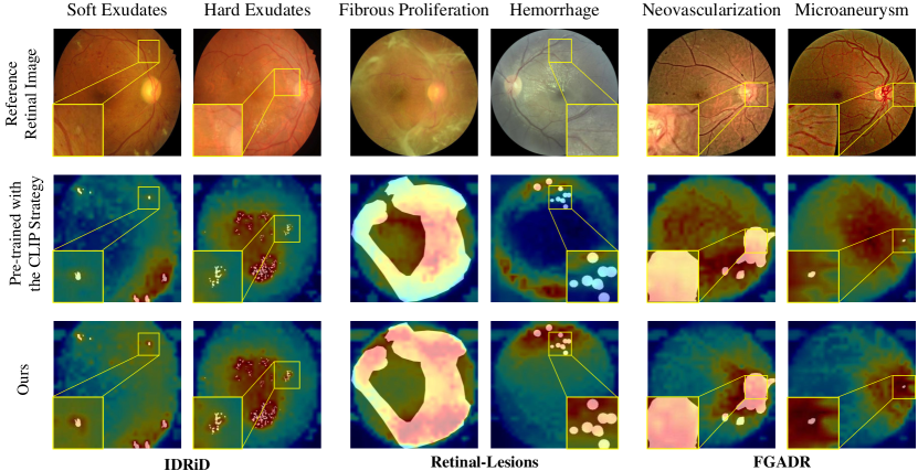
Figure 3: Visualization of multi-modal activation maps for model pre-trained with the CLIP strategy and ours on IDRiD (exemplar: soft exudates and hard exducates), Retinal-Lesions (exemplar: fibrous proliferation and hemorrhage), and FGADR (exemplar: neovascularization and microaneurysm). The white mask area indicates the ground truth.

IV-C2 Results on fully fine-tuned classification

We apply fully fine-tuned classification tasks, comparing our pre-training strategy with existing methods on test datasets. The results are shown in Table III. From the experimental results, we can draw conclusions consistent with those from the linear probing: the model pre-trained with our strategy demonstrates superior performance accross all test datasets. This shows that our pre-training strategy not only enables the model to learn rich and high-quality representations in the pre-training stage but also has strong generalization performance during specific downstream tasks.

IV-C3 Results on prompt-based OOD-ZSC

We apply prompt-based OOD-ZSC to evaluate the feature extraction quality and the visual-language representation alignment performance. The results are presented in Table IV. The MAE strategy does not involve text and is therefore excluded from this comparison.

The CLIP strategy introduces noise into the model due to false negatives, complicating the matching of images and texts with the same semantics. The DeiT strategy shows poor performance in cross-modal alignment because the distillation constraint introduces uncertainty. The MedCLIP strategy, which aligns feature similarities with label similarities, enables the model to achieve good performance on some test datasets. For example, it achieves an mAP of $59.57\%$ on ODIR. However, during the pre-training stage, the samples categorized in different grades of DR are assigned to the same label and are optimized to be similar in the feature space, leading to false positive samples in the DR grading task and thus causing lower performance of AUC.

For these potential false positive samples in downstream tasks with more subdivided categories, our pre-training strategy eliminates them rather than forcing them to be similar. This approach enables the model to adapt to various downstream tasks effectively. Our pre-training strategy allows the model to achieve the best overall performance and distinguish diseases in different grades, as demonstrated by the superior AUC of $72.25\%$ and mAP of $47.73\%$ on the DR grading task on MESSIDOR dataset, surpassing the second-best CLIP-based model by $13.57\%$ and $13.41\%$, respectively.

IV-C4 Multi-modal activation map visualization using Grad-CAM

To demonstrate the interpretability of features extracted by ViLReF more intuitively, we adopt the multi-modal Grad-CAM method to visualize the gradient activation heatmaps. The multi-modal heatmap overlays are drawn on IDRiD, Retinal-Lesions, and FGADR datasets, as shown in Fig. 3, with one sample for each disease. Due to space limitations, we only show the results for ViLReF and the runner-up model pre-trained with the CLIP strategy. Owing to the additional supervision provided by labels and the proposed Weighted Similarity Coupling Loss, ViLReF can learn the lesion features of retinal images more effectively, which can be reflected in the more accurate activation positions of the lesion appearance, location, and extent. Additionally, ViLReF is capable of learning more subtle lesion patterns.

IV-D Ablation Study

To evaluate the contribution of each component in our pre-training strategy, we conduct ablation studies using the same pre-training data and fix the image encoder to ViT-B/16 as in previous evaluations. We introduce the speed adjustment of feature similarity (SA) and the batch expansion (BE) to the baseline CN-CLIP. We then compare their performance on two downstream tasks: fully fine-tuned classification and prompt-based OOD-ZSC.

TABLE V: Evaluation on Fully Fine-tuned Classification Performance for Ablation Study. Each Encoder is Fixed to Vit-B/16. (%)

	AUC				mAP
SA	✗	✗	✓	✔	✗	✗	✓	✔
BE	✗	✓	✗	✔	✗	✓	✗	✔
RFMiD	94.61 (0.11)	94.49 (0.08)	94.79 (0.21)	95.17 (0.09)	63.00 (0.26)	63.21 (0.30)	63.19 (0.18)	66.17 (0.15)
ODIR	92.73 (0.38)	92.11 (0.34)	92.43 (0.13)	93.01 (0.11)	71.39 (0.70)	70.11 (0.55)	71.45 (0.56)	71.54 (0.16)
REFUGE	96.63 (0.44)	96.58 (1.37)	97.20 (0.37)	97.73 (0.30)	94.97 (0.51)	94.89 (0.89)	95.05 (0.30)	95.23 (0.15)
MESSIDOR	84.81 (0.71)	84.52 (0.45)	85.37 (0.77)	86.29 (0.40)	63.19 (0.52)	62.09 (0.26)	64.12 (0.57)	65.02 (0.37)
FIVES	97.48 (0.35)	96.49 (0.17)	97.82 (0.20)	98.13 (0.11)	94.48 (0.63)	91.54 (0.40)	95.11 (0.33)	95.56 (0.22)

TABLE VI: Evaluation on Prompt-based OOD-ZSC Performance for Ablation Study. Each Encoder is Fixed to Vit-B/16. (%)

	AUC				mAP
SA	✗	✗	✓	✔	✗	✗	✓	✔
BE	✗	✓	✗	✔	✗	✓	✗	✔
RFMiD	82.32	80.86	85.08	84.82	35.27	36.38	37.54	37.57
ODIR	86.11	81.28	88.43	88.73	54.26	54.99	58.36	58.99
REFUGE	83.37	86.48	87.55	93.18	82.14	79.11	85.08	86.78
MESSIDOR	58.68	65.07	71.70	72.25	34.32	37.09	45.74	47.73
FIVES	89.98	92.17	93.70	93.67	76.39	81.03	84.70	84.72

• Obtaining the mean and standard deviation from five repeated runs is not applicable to prompt-based OOD-ZSC because all parameters are fixed.

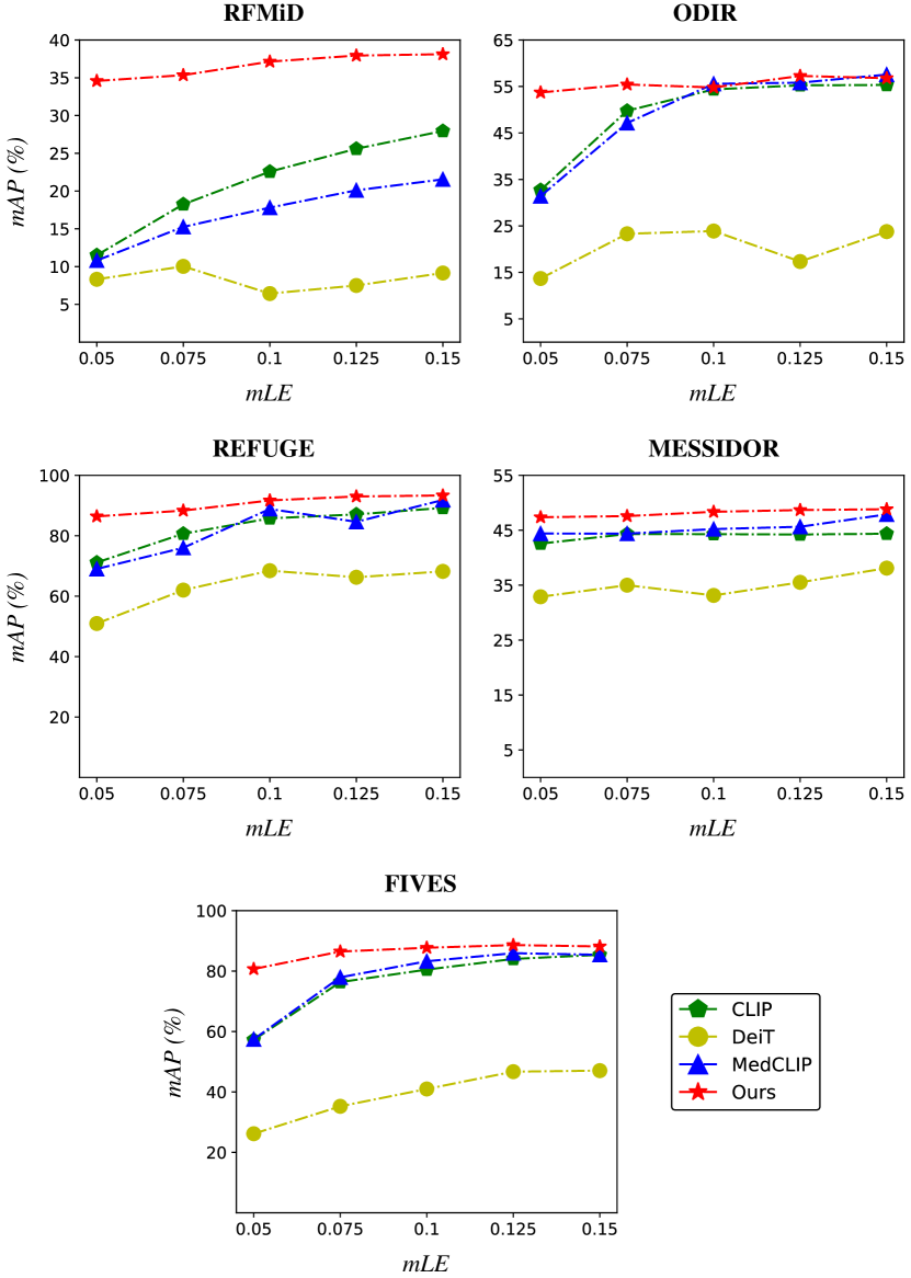
Figure 4: Comparison of prompt-based OOD-ZSC performance for models trained on datasets with different label entropies.

IV-D1 Results on fully fine-tuned classification

The results of fully fine-tuned classification performance are shown in Table V. Without applying SA, only employing BE does not improve the performance significantly, as it does not address the impact of false negative samples. On the other hand, applying SA alone can improve the model’s performance significantly. For instance, the AUC on REFUGE increases to $97.20\%$, which is $0.57\%$ higher than the baseline, and the mAP on FIVES imcreases to $95.11\%$, with an improvement of $0.63\%$. When both SA and BE are employed, the model achieves the best performance across all datasets. This indicates that the dynamic memory queues effectively compensate for the vacancies caused by eliminating false negatives.

IV-D2 Results on prompt-based OOD-ZSC

The results of prompt-based OOD-ZSC performance are shown in Table VI. From the experimental results, we can draw conclusions consistent with those from the fully fine-tuned task. As expected, the combination of SA and BE leads to the most significant improvement across all datasets.

These ablation studies highlight the synergistic effect of the two crucial components of our pre-training strategy in improving the model’s ability to capture and understand generalizable representations within ophthalmic data, while maintaining strong alignment between visual and language representations across diverse datasets.

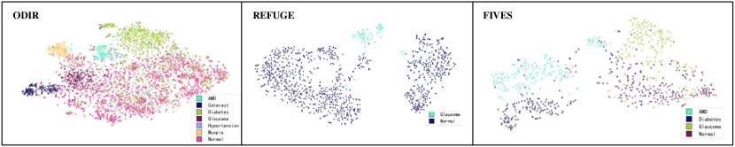
Figure 5: Visualization of compressed feature distributions encoded by ViLReF on ODIR, REFUGE and FIVES datasets via t-SNE dimensionality reduction.

TABLE VII: Evaluation on Fully Fine-tuned Classification Performance for Different Retinal Foundation Models. (%)

Model	Visual architecture	RFMiD		ODIR		REFUGE		MESSIDOR		FIVES
		AUC	mAP	AUC	mAP	AUC	mAP	AUC	mAP	AUC	mAP
FLAIR	ResNet50	79.78 (0.37)	33.24 (0.12)	83.44 (0.46)	58.97 (0.21)	92.54 (2.85)	89.78 (1.89)	77.37 (1.52)	58.00 (0.62)	91.84 (1.54)	86.89 (1.42)
KeepFIT (CFP)	ResNet50	87.25 (0.24)	40.93 (0.11)	86.74 (0.50)	59.36 (0.19)	85.73 (1.90)	81.88 (0.85)	80.19 (0.29)	58.35 (0.16)	95.00 (0.20)	88.67 (0.45)
RETFound (CFP)	ViT-L/16	90.60 (0.21)	53.12 (0.41)	88.53 (0.68)	64.51 (0.32)	94.50 (1.14)	91.52 (2.14)	79.03 (1.52)	56.32 (1.34)	96.94 (0.36)	92.87 (0.77)
RET-CLIP	ViT-B/16	94.22 (0.41)	61.39 (0.15)	92.61 (0.32)	69.56 (0.69)	95.68 (0.19)	94.42 (0.25)	84.20 (0.22)	61.77 (0.34)	97.06 (0.26)	93.84 (0.26)
ViLReF (RN50)	ResNet50	93.51 (0.13)	60.15 (0.28)	93.60 (0.08)	73.69 (0.25)	97.72 (0.32)	94.03 (0.15)	88.18 (0.16)	68.89 (0.20)	97.55 (0.29)	93.82 (0.71)
ViLReF (ViT-B/16)	ViT-B/16	95.17 (0.09)	66.17 (0.15)	93.01 (0.11)	71.54 (0.16)	97.73 (0.30)	95.23 (0.15)	86.29 (0.40)	65.02 (0.37)	98.13 (0.11)	95.56 (0.22)

IV-E Further Discussion on Pre-Training Effectiveness

In this section, we further discuss the effectiveness of our pre-training strategy. We introduce mean label entropy (mLE) to evaluate the impact of training data with different proportions of identical labels on pre-training. Additionally, we visualize the clustering patterns of distributions in the feature space using t-distributed Stochastic Neighbor Embedding (t-SNE) [54], which helps validate whether our pre-training strategy separates images of different categories correctly and aggregates those of the same category.

IV-E1 Label Entropy Analysis

We sample subsets containing 100,000 image-text pairs with different mLEs from the full pre-training dataset to pre-train the model. The mLE is calculated as:

$$mLE=-\frac{1}{c}\sum_{i}\left[P(y_{i}=1)\log P(y_{i}=1)\right.\\ \left.+P(y_{i}=0)\log P(y_{i}=0)\right].$$ (14)

When the mLE of a dataset is high, the proportion of identical labels is low; when the mLE is low, the proportion of identical labels is high. The mLE of full pre-training dataset is $0.1423$, while the sampled subsets are $0.05$, $0.075$, $0.1$, $0.125$, and $0.15$, respectively. We investigate the changes in the prompt-based OOD-ZSC performance for models pre-trained with different strategies as the mLE of the pre-training dataset varies. The results are depicted in Fig. 4.

It can be observed that the performance of the four pre-training strategies improves with the increase of mLE. Among them, the CLIP and MedCLIP strategies are affected significantly, indicating that neither can mitigate the impact caused by false negative samples effectively. The results of DeiT further demonstrate the aforementioned declaration that the distillation constraint introduces uncertainty. Regardless of the mLE value of the pre-training dataset, our strategy achieves the best prompt-based OOD-ZSC performance. Notably, when the mLE value is $0.05$, our strategy outperforms the comparison methods significantly, validating that the additional supervision can guide the optimization direction of contrastive learning effectively, enabling it to learn effective representations from datasets with highly similar labels.

IV-E2 Feature visualization using t-SNE

To demonstrate that ViLReF, pre-trained using the proposed strategy, can effectively capture discriminative features in retinal images and possess strong generalization capabilities, we employ the t-SNE method to visualize the multi-class clusters in the ODIR, REFUGE, and FIVES datasets, as shown in Fig. 5. It can be observed that ViLReF effectively clusters retinal images belonging to different diseases. Although retinal image features are highly homogeneous compared with natural image features due to the high consistency of image structure and content, ViLReF still achieves good classification results on downstream tasks.

TABLE VIII: Evaluation on Fully Fine-tuned Lesion Segmentation Performance for Different Pre-trained Encoders. Each Encoder is Fixed to ResNet50. (%)

Pre-trained Visual Encoder	Hemorrhages
	IDRiD		Retinal-Lesions		FGADR
	DSC	IoU	DSC	IoU	DSC	IoU
CN-CLIP (RN50)	51.84 (0.72)	37.64 (0.56)	34.22 (0.04)	23.35 (0.09)	37.77 (0.16)	26.06 (0.11)
FLAIR	48.21 (0.89)	33.92 (0.90)	31.76 (0.51)	21.40 (0.30)	36.35 (0.46)	24.85 (0.35)
KeepFIT (CFP)	41.29 (1.15)	29.41 (0.71)	31.75 (0.15)	21.39 (0.18)	36.00 (0.22)	24.54 (0.18)
ViLReF (RN50)	52.65 (0.86)	38.38 (0.60)	34.35 (0.09)	23.44 (0.06)	38.23 (0.48)	26.46 (0.33)
Pre-trained Visual Encoder	Soft Exudates
	IDRiD		Retinal-Lesions		FGADR
	DSC	IoU	DSC	IoU	DSC	IoU
CN-CLIP (RN50)	59.50 (1.13)	47.23 (1.71)	48.22 (0.34)	35.75 (0.24)	35.43 (0.60)	25.75 (0.58)
FLAIR	58.02 (1.30)	45.12 (1.77)	48.13 (0.63)	35.58 (0.50)	33.38 (0.98)	24.28 (0.75)
KeepFIT (CFP)	58.40 (0.65)	45.69 (0.73)	47.43 (0.46)	34.58 (0.26)	33.47 (0.62)	24.38 (0.61)
ViLReF (RN50)	60.05 (1.03)	47.86 (1.02)	49.43 (0.51)	36.73 (0.35)	36.11 (0.74)	26.32 (0.63)
Pre-trained Visual Encoder	Hard Exudates
	IDRiD		Retinal-Lesions		FGADR
	DSC	IoU	DSC	IoU	DSC	IoU
CN-CLIP (RN50)	55.18 (0.66)	40.79 (0.41)	46.16 (0.40)	34.35 (0.33)	44.01 (0.17)	31.08 (0.22)
FLAIR	54.75 (0.71)	40.90 (0.52)	47.38 (0.30)	35.47 (0.32)	44.30 (0.74)	31.20 (0.47)
KeepFIT (CFP)	54.88 (0.38)	40.08 (0.20)	48.23 (0.23)	36.07 (0.17)	44.93 (0.38)	31.77 (0.20)
ViLReF (RN50)	56.53 (0.18)	41.50 (0.13)	46.46 (0.24)	34.59 (0.29)	44.38 (0.22)	32.00 (1.30)

IV-F Comparison with State-of-the-art Models

In this section, we compare the performance of our model with state-of-the-art foundation models pre-trained on various data domains:

• FLAIR [35] is pre-trained on a collection of 37 datasets comprising 284,660 retinal images in 96 categories with different distributions. The diagnostic reports are synthesized from labels by leveraging expert knowledge.

• KeepFIT [36] employs MM-Retinal, a multi-modal dataset containing color fundus photography (CFP) and FFA image-text pairs captured from 4 professional fundus diagram books, to leverage expert knowledge to enhance the representation learning. We use its CFP version for evaluation.

• RETFound [14] includes 2 versions pre-trained with masked autoencoders, one pre-trained on 904,170 CFP images and the other on 736,442 optical coherence tomography (OCT) images. We use its CFP version for evaluation.

• RET-CLIP [29] is pre-trained on a retinal image-text dataset of 193,865 patients, optimizing feature extraction at the left eye, right eye, and patient levels, respectively.

IV-F1 Results on fully fine-tuned classification

We compare the fully fine-tuned classification performance of ViLReF and state-of-the-art retinal foundation models on test datasets. For fair and adequate comparison with existing models, we train a version of ViLReF using ResNet50 [55] as the image encoder additionally. The results are presented in Table VII.

FLAIR is pre-trained using the CLIP strategy, which is prone to false negatives. Additionally, FLAIR is pre-trained on a dataset using synthesized text reports based on labels, which lacks clinical diversity. Moreover, the combination of multiple small-scale public datasets suffers from poor data quality, limiting the model’s performance. KeepFIT achieves better overall performance due to the incorporation of expert knowledge into the pre-training dataset used by FLAIR. Since RETFound is pre-trained using the MAE strategy, its performance is not very satisfactory. RET-CLIP, pre-trained on a high-quality, large-scale retinal image-text dataset, learns representations at both monocular and binocular levels innovatively, achieving higher performance. However, it cannot alleviate the impact of false negative samples.

Our ViLReF demonstrates overwhelmingly high fully fine-tuned classification performance, surpassing the state-of-the-art retinal foundation models. Specifically, the ResNet50 version achieves an mAP of $73.69\%$ on ODIR dataset, an AUC of $88.18\%$, and an mAP of $68.89\%$ on MESSIDOR dataset, surpassing the runner-up ResNet50-based KeepFIT by $14.33\%$, $7.99\%$, and $10.54\%$, respectively. The ViT version achieves an mAP of $66.17\%$ on RFMiD, which is $4.78\%$ higher than the second-place ViT-based RET-CLIP. Both versions far outperform other state-of-the-art models under the same visual architecture.

IV-F2 Results on fully fine-tuned lesion segmentation

We evaluate the fully fine-tuned lesion segmentation performance on hemorrhages, soft exudates, and hard exudates across IDRiD, Retinal-Lesions, and FGADR datasets. For fair comparison using the same segmentation decoder, we use the ResNet50 version of ViLReF and compare its visual encoder with those of CN-CLIP, FLAIR, and KeepFIT, which also use ResNet50. The experimental results are presented in Table VIII, covering segmentation performance on three types of lesions: hemorrhages, soft exudates, and hard exudates across IDRiD, Retinal-Lesions, and FGADR datasets. It can be observed that using ViLReF’s visual encoder overall enhances the segmentation performance. Both DSC and IoU scores surpass or achieve comparable results with the state-of-the-art retinal foundation models. The results demonstrate that the representations learned by ViLReF are of high quality and have strong generalization ability.

V Conclusion

In this work, we propose ViLReF, a model pre-trained on 451,956 paired retinal image-diagnostic text report data. Expert knowledge is leveraged to guide label extraction, enabling the model to capture subtle but clinically significant visual patterns in retinal images. We present a novel Weighted Similarity Coupling Loss, $\mathcal{L}_{WSC}$, to adjust the speed of pushing sample pairs further apart dynamically within the feature space. Furthermore, a batch expansion module with dynamic memory queues is utilized to mitigate the equivalent batch size reduction incurred by eliminating false negative samples. Compared with state-of-the-art foundation models, our proposed ViLReF demonstrates superior representation learning performance and more promising results on various downstream tasks. In future work, we will explore more effective ways to utilize data information and further investigate the model’s capabilities on more complex datasets.

References

- [1] M. Moor, O. Banerjee, Z. S. H. Abad, H. M. Krumholz, J. Leskovec, E. J. Topol, and P. Rajpurkar, “Foundation models for generalist medical artificial intelligence,” Nature, vol. 616, no. 7956, pp. 259–265, 2023.
- [2] A. Radford, J. W. Kim, C. Hallacy, A. Ramesh, G. Goh, S. Agarwal, G. Sastry, A. Askell, P. Mishkin, J. Clark, et al., “Learning transferable visual models from natural language supervision,” in International Conference on Machine Learning, pp. 8748–8763, PMLR, 2021.
- [3] Z. Wang, Z. Wu, D. Agarwal, and J. Sun, “Medclip: Contrastive learning from unpaired medical images and text,” arXiv preprint arXiv:2210.10163, 2022.
- [4] S.-C. Huang, L. Shen, M. P. Lungren, and S. Yeung, “Gloria: A multimodal global-local representation learning framework for label-efficient medical image recognition,” in Proceedings of the IEEE/CVF International Conference on Computer Vision, pp. 3942–3951, 2021.
- [5] Y. Lv, J. Zhang, N. Barnes, and Y. Dai, “Weakly-supervised contrastive learning for unsupervised object discovery,” IEEE Transactions on Image Processing, 2024.
- [6] O. Bodenreider, “The unified medical language system (umls): integrating biomedical terminology,” Nucleic Acids Research, vol. 32, no. suppl_1, pp. D267–D270, 2004.
- [7] S. Zhang and N. Elhadad, “Unsupervised biomedical named entity recognition: Experiments with clinical and biological texts,” Journal of Biomedical Informatics, vol. 46, no. 6, pp. 1088–1098, 2013.
- [8] L. Chen, Y. Qi, A. Wu, L. Deng, and T. Jiang, “Mapping chinese medical entities to the unified medical language system,” Health Data Science, vol. 3, p. 0011, 2023.
- [9] D. Erhan, P.-A. Manzagol, Y. Bengio, S. Bengio, and P. Vincent, “The difficulty of training deep architectures and the effect of unsupervised pre-training,” in Artificial Intelligence and Statistics, pp. 153–160, PMLR, 2009.
- [10] A. Jaiswal, A. R. Babu, M. Z. Zadeh, D. Banerjee, and F. Makedon, “A survey on contrastive self-supervised learning,” Technologies, vol. 9, no. 1, p. 2, 2020.
- [11] C. Yang, Z. Wu, B. Zhou, and S. Lin, “Instance localization for self-supervised detection pretraining,” in Proceedings of the IEEE/CVF Conference on Computer Vision and Pattern Recognition, pp. 3987–3996, 2021.
- [12] Q. Cai, Y. Qian, J. Li, J. Lyu, Y.-H. Yang, F. Wu, and D. Zhang, “Hipa: hierarchical patch transformer for single image super resolution,” IEEE Transactions on Image Processing, 2023.
- [13] X. Yang, J. Fan, C. Wu, D. Zhou, and T. Li, “Nasmamsr: a fast image super-resolution network based on neural architecture search and multiple attention mechanism,” Multimedia Systems, pp. 1–14, 2022.
- [14] Y. Zhou, M. A. Chia, S. K. Wagner, M. S. Ayhan, D. J. Williamson, R. R. Struyven, T. Liu, M. Xu, M. G. Lozano, P. Woodward-Court, et al., “A foundation model for generalizable disease detection from retinal images,” Nature, vol. 622, no. 7981, pp. 156–163, 2023.
- [15] D. Shi, W. Zhang, X. Chen, Y. Liu, J. Yang, S. Huang, Y. C. Tham, Y. Zheng, and M. He, “Eyefound: A multimodal generalist foundation model for ophthalmic imaging,” arXiv preprint arXiv:2405.11338, 2024.
- [16] K. He, X. Chen, S. Xie, Y. Li, P. Dollár, and R. Girshick, “Masked autoencoders are scalable vision learners,” in Proceedings of the IEEE/CVF Conference on Computer Vision and Pattern Recognition, pp. 16000–16009, 2022.
- [17] L. Ericsson, H. Gouk, C. C. Loy, and T. M. Hospedales, “Self-supervised representation learning: Introduction, advances, and challenges,” IEEE Signal Processing Magazine, vol. 39, no. 3, pp. 42–62, 2022.
- [18] T. Chen, S. Kornblith, M. Norouzi, and G. Hinton, “A simple framework for contrastive learning of visual representations,” in International Conference on Machine Learning, pp. 1597–1607, PMLR, 2020.
- [19] K. He, H. Fan, Y. Wu, S. Xie, and R. Girshick, “Momentum contrast for unsupervised visual representation learning,” in Proceedings of the IEEE/CVF Conference on Computer Vision and Pattern Recognition, pp. 9729–9738, 2020.
- [20] M. Caron, H. Touvron, I. Misra, H. Jégou, J. Mairal, P. Bojanowski, and A. Joulin, “Emerging properties in self-supervised vision transformers,” in Proceedings of the IEEE/CVF International Conference on Computer Vision, pp. 9650–9660, 2021.
- [21] M. Caron, I. Misra, J. Mairal, P. Goyal, P. Bojanowski, and A. Joulin, “Unsupervised learning of visual features by contrasting cluster assignments,” Advances in Neural Information Processing Systems, vol. 33, pp. 9912–9924, 2020.
- [22] J. Li, P. Zhou, C. Xiong, and S. C. Hoi, “Prototypical contrastive learning of unsupervised representations,” arXiv preprint arXiv:2005.04966, 2020.
- [23] A. E. Johnson, T. J. Pollard, S. J. Berkowitz, N. R. Greenbaum, M. P. Lungren, C.-y. Deng, R. G. Mark, and S. Horng, “Mimic-cxr, a de-identified publicly available database of chest radiographs with free-text reports,” Scientific Data, vol. 6, no. 1, p. 317, 2019.
- [24] A. Bustos, A. Pertusa, J.-M. Salinas, and M. De La Iglesia-Vaya, “Padchest: A large chest x-ray image dataset with multi-label annotated reports,” Medical Image Analysis, vol. 66, p. 101797, 2020.
- [25] O. Pelka, S. Koitka, J. Rückert, F. Nensa, and C. M. Friedrich, “Radiology objects in context (roco): a multimodal image dataset,” in Intravascular Imaging and Computer Assisted Stenting and Large-Scale Annotation of Biomedical Data and Expert Label Synthesis, pp. 180–189, Springer, 2018.
- [26] Y. Zhang, H. Jiang, Y. Miura, C. D. Manning, and C. P. Langlotz, “Contrastive learning of medical visual representations from paired images and text,” in Machine Learning for Healthcare Conference, pp. 2–25, PMLR, 2022.
- [27] S. Zhang, Y. Xu, N. Usuyama, J. Bagga, R. Tinn, S. Preston, R. Rao, M. Wei, N. Valluri, C. Wong, et al., “Large-scale domain-specific pretraining for biomedical vision-language processing,” arXiv preprint arXiv:2303.00915, vol. 2, no. 3, p. 6, 2023.
- [28] M. Wang, T. Lin, K. Yu, A. Lin, Y. Peng, L. Wang, C. Chen, K. Zou, H. Liang, M. Chen, et al., “Common and rare fundus diseases identification using vision-language foundation model with knowledge of over 400 diseases,” arXiv preprint arXiv:2406.09317, 2024.
- [29] J. Du, J. Guo, W. Zhang, S. Yang, H. Liu, H. Li, and N. Wang, “Ret-clip: A retinal image foundation model pre-trained with clinical diagnostic reports,” arXiv preprint arXiv:2405.14137, 2024.
- [30] S. Sivaprasad, S. Sen, and J. Cunha-Vaz, “Perspectives of diabetic retinopathy—challenges and opportunities,” Eye, vol. 37, no. 11, pp. 2183–2191, 2023.
- [31] M. Fleckenstein, S. Schmitz-Valckenberg, and U. Chakravarthy, “Age-related macular degeneration: A review,” JAMA, vol. 331, no. 2, pp. 147–157, 2024.
- [32] L. Giancardo, F. Meriaudeau, T. P. Karnowski, Y. Li, S. Garg, K. W. Tobin Jr, and E. Chaum, “Exudate-based diabetic macular edema detection in fundus images using publicly available datasets,” Medical Image Analysis, vol. 16, no. 1, pp. 216–226, 2012.
- [33] S. Lu, H. Zhao, H. Liu, H. Li, and N. Wang, “Pkrt-net: prior knowledge-based relation transformer network for optic cup and disc segmentation,” Neurocomputing, vol. 538, p. 126183, 2023.
- [34] C. Wu, X. Zhang, Y. Zhang, Y. Wang, and W. Xie, “Medklip: Medical knowledge enhanced language-image pre-training,” medRxiv, pp. 2023–01, 2023.
- [35] J. Silva-Rodriguez, H. Chakor, R. Kobbi, J. Dolz, and I. B. Ayed, “A foundation language-image model of the retina (flair): Encoding expert knowledge in text supervision,” arXiv preprint arXiv:2308.07898, 2023.
- [36] R. Wu, C. Zhang, J. Zhang, Y. Zhou, T. Zhou, and H. Fu, “Mm-retinal: Knowledge-enhanced foundational pretraining with fundus image-text expertise,” arXiv preprint arXiv:2405.11793, 2024.
- [37] R. Luo, J. Xu, Y. Zhang, Z. Zhang, X. Ren, and X. Sun, “Pkuseg: A toolkit for multi-domain chinese word segmentation,” arXiv preprint arXiv:1906.11455, 2019.
- [38] K. Gupta, T. Ajanthan, A. v. d. Hengel, and S. Gould, “Understanding and improving the role of projection head in self-supervised learning,” arXiv preprint arXiv:2212.11491, 2022.
- [39] S. Pachade, P. Porwal, D. Thulkar, M. Kokare, G. Deshmukh, V. Sahasrabuddhe, L. Giancardo, G. Quellec, and F. Mériaudeau, “Retinal fundus multi-disease image dataset (rfmid): A dataset for multi-disease detection research,” Data, vol. 6, no. 2, p. 14, 2021.
- [40] “Peking university international competition on ocular disease intelligent recognition (odir-2019),” https://odir2019.grandchallenge.org/.
- [41] J. I. Orlando, H. Fu, J. B. Breda, K. Van Keer, D. R. Bathula, A. Diaz-Pinto, R. Fang, P.-A. Heng, J. Kim, J. Lee, et al., “Refuge challenge: A unified framework for evaluating automated methods for glaucoma assessment from fundus photographs,” Medical Image Analysis, vol. 59, p. 101570, 2020.
- [42] E. Decencière, X. Zhang, G. Cazuguel, B. Lay, B. Cochener, C. Trone, P. Gain, R. Ordonez, P. Massin, A. Erginay, et al., “Feedback on a publicly distributed image database: the messidor database,” Image Analysis and Stereology, vol. 33, no. 3, pp. 231–234, 2014.
- [43] K. Jin, X. Huang, J. Zhou, Y. Li, Y. Yan, Y. Sun, Q. Zhang, Y. Wang, and J. Ye, “Fives: A fundus image dataset for artificial intelligence based vessel segmentation,” Scientific Data, vol. 9, no. 1, p. 475, 2022.
- [44] P. Porwal, S. Pachade, R. Kamble, M. Kokare, G. Deshmukh, V. Sahasrabuddhe, and F. Meriaudeau, “Indian diabetic retinopathy image dataset (idrid): a database for diabetic retinopathy screening research,” Data, vol. 3, no. 3, p. 25, 2018.
- [45] Q. Wei, X. Li, W. Yu, X. Zhang, Y. Zhang, B. Hu, B. Mo, D. Gong, N. Chen, D. Ding, and Y. Chen, “Learn to segment retinal lesions and beyond,” in International Conference on Pattern Recognition, 2020.
- [46] Y. Zhou, B. Wang, L. Huang, S. Cui, and L. Shao, “A benchmark for studying diabetic retinopathy: Segmentation, grading, and transferability,” IEEE Transactions on Medical Imaging, vol. 40, no. 3, pp. 818–828, 2021.
- [47] A. Yang, J. Pan, J. Lin, R. Men, Y. Zhang, J. Zhou, and C. Zhou, “Chinese clip: Contrastive vision-language pretraining in chinese,” arXiv preprint arXiv:2211.01335, 2022.
- [48] A. Dosovitskiy, L. Beyer, A. Kolesnikov, D. Weissenborn, X. Zhai, T. Unterthiner, M. Dehghani, M. Minderer, G. Heigold, S. Gelly, et al., “An image is worth 16x16 words: Transformers for image recognition at scale,” arXiv preprint arXiv:2010.11929, 2020.
- [49] Y. Cui, W. Che, T. Liu, B. Qin, S. Wang, and G. Hu, “Revisiting pre-trained models for chinese natural language processing,” arXiv preprint arXiv:2004.13922, 2020.
- [50] X. Li, Y. Meng, X. Sun, Q. Han, A. Yuan, and J. Li, “Is word segmentation necessary for deep learning of chinese representations?,” arXiv preprint arXiv:1905.05526, 2019.
- [51] I. Loshchilov and F. Hutter, “Decoupled weight decay regularization,” arXiv preprint arXiv:1711.05101, 2017.
- [52] H. Touvron, M. Cord, M. Douze, F. Massa, A. Sablayrolles, and H. Jegou, “Training data-efficient image transformers & distillation through attention,” in International Conference on Machine Learning, vol. 139, pp. 10347–10357, July 2021.
- [53] R. R. Selvaraju, M. Cogswell, A. Das, R. Vedantam, D. Parikh, and D. Batra, “Grad-cam: Visual explanations from deep networks via gradient-based localization,” in Proceedings of the IEEE International Conference on Computer Vision, pp. 618–626, 2017.
- [54] L. Van der Maaten and G. Hinton, “Visualizing data using t-sne.,” Journal of Machine Learning Research, vol. 9, no. 11, 2008.
- [55] K. He, X. Zhang, S. Ren, and J. Sun, “Deep residual learning for image recognition,” in Proceedings of the IEEE Conference on Computer Vision and Pattern Recognition, pp. 770–778, 2016.