TANGO: Clustering with Typicality-Aware Nonlocal Mode-Seeking and Graph-Cut Optimization

Abstract

Density-based clustering methods by mode-seeking usually achieve clustering by using local density estimation to mine structural information, such as local dependencies from lower density points to higher neighbors. However, they often rely too heavily on local structures and neglect global characteristics, which can lead to significant errors in peak selection and dependency establishment. Although introducing more hyperparameters that revise dependencies can help mitigate this issue, tuning them is challenging and even impossible on real-world datasets. In this paper, we propose a new algorithm (TANGO) to establish local dependencies by exploiting a global-view typicality of points, which is obtained by mining further the density distributions and initial dependencies. TANGO then obtains sub-clusters with the help of the adjusted dependencies, and characterizes the similarity between sub-clusters by incorporating path-based connectivity. It achieves final clustering by employing graph-cut on sub-clusters, thus avoiding the challenging selection of cluster centers. Moreover, this paper provides theoretical analysis and an efficient method for the calculation of typicality. Experimental results on several synthetic and $16$ real-world datasets demonstrate the effectiveness and superiority of TANGO.

Introduction

Density-based clustering methods (Hartigan 1975; Ester et al. 1996; Tobin and Zhang 2024) have gained wide attention and thorough investigation due to their capability in handling complex data distributions. Mean Shift (Cheng 1995) and Quick Shift (Vedaldi and Soatto 2008) are the most representative density-based mode-seeking methods. Mean Shift iteratively converges data points into multiple clusters along the path of the steepest ascent of the density function. In contrast, Quick Shift enhances efficiency by establishing local dependencies through directly linking each sample point to the nearest neighbor with higher density that is within its $\tau$-radius neighborhood, eliminating the iterative process of Mean Shift. However, Quick Shift is highly sensitive to the hyperparameter $\tau$, and determining it without prior information still remains challenging.

Building upon this, the Density Peaks Clustering (DPC) algorithm (Rodriguez and Laio 2014) introduces a novel approach where modes of the data (cluster centers), are selected based on a decision graph given by both the local density $\rho$ and the distance $\delta$ to the nearest point with higher density. Each non-center point forms a dependency relationship with another point like Quick Shift, ultimately connecting to a mode (cluster center) along a density ascent path to complete clustering. Subsequent researchers have proposed various improvements of DPC tailored for manifold-structured, unevenly dense, and noisy data (Liu, Wang, and Yu 2018; Wang et al. 2023). However, a significant drawback of these methods is that selecting modes and establishing dependencies are both based on local data structures, lacking global perspective, which potentially lead to errors in complex data.

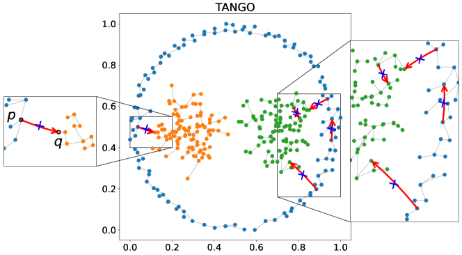
Figure 1: The existing issues with the Mode-Seeking paradigm and improvements related to the typicality proposed in this paper.

As shown in Fig. 1, due to significant density differences between clusters in the dataset, the existing Mode-Seeking paradigm can lead to incorrect dependency relationships (such as the connection indicated by the red arrow between points $p$ and $q$). In fact, point $p$ is one of the key points in a low-density region, whereas point $q$, although its density is higher than $p$, is not a key point in a high-density region. Such incorrect connection can lead to the merging of the two regions, thereby compromising clustering effectiveness. While some studies (Jiang, Jang, and Kpotufe 2018; Wang et al. 2023) have introduced more hyperparameters to prevent such connections, tuning them remains challenging and using the same hyperparameter value across different regions of complex data is also usually impractical.

To resolve these issues, it is useful to explore the internal structure of the data from a global perspective. As shown in Fig. 1, from a global perspective, point $p$ receives dependencies from more low-density points, whereas point $q$ is dependent by only very few points. In other words, the confidence of $p$ being a representative point should be higher than that of $q$. Therefore, based on density and dependency relationships, we propose to mine high-order features of the data and introduce the concept of typicality to help detect and remove potentially incorrect dependency connections between data points.

In addition, for complex data where determining the cluster centers is challenging, we employ graph-cut (Ng, Jordan, and Weiss 2001) to avoid the selection of cluster centroids for final clustering. Specifically, we first partition the data into tree-like sub-clusters by leveraging the dependency relationships adjusted by the proposed typicality; then, the similarities between sub-clusters are measured from a path-based connectivity perspective (Fischer, Roth, and Buhmann 2003); and finally, by using a global graph cut method, we aggregate the sub-clusters to achieve the final clustering result.

The contributions of this paper are as follows:

• By integrating local data similarities and overall distribution characteristics, a new clustering framework that fuses local and global information is proposed, introducing a new global perspective into density-based clustering methods.

• We introduce typicality to automatically exclude potentially incorrect dependency relationships in a parameter-free manner. Constraining equations for typicality are formulated, and the uniqueness and computational efficiency of typicality based on common dependency relationship are theoretically proven.

• Improved path-based similarities are utilized to comprehensively estimate similarities between sub-clusters. Graph-cut is employed to avoid the challenge of selecting cluster centroids on complex datasets.

The rest of this paper is organized as follows: The next section reviews related work, and then we present the details of the proposed TANGO algorithm, followed by a comparison of TANGO with multiple state-of-the-art algorithms on extensive datasets through experiments.

Related Work

Density-based clustering by mode-seeking relies on density estimation, identification of modes (e.g., density peaks), and establishment of dependency relationships.

The earlier Mean Shift (Cheng 1995) iteratively moves each data point to the mean of its neighborhood, which is equivalent to establishing dependency relationships in the direction of the steepest ascent of density (Arias-Castro, Mason, and Pelletier 2016). Quick Shift (Vedaldi and Soatto 2008) establishes dependency relationships by directly associating each point with its nearest neighbor of higher density, and identifies modes as points not dependending on others, which significantly accelerates Mean Shift. HQuickShift (Altinigneli et al. 2020) integrates hierarchical clustering with Quick Shift and a Mode Attraction Graph to help determine the hyperparameter for establishing dependencies, to deal with the sensitivity to hyperparameters of Quick Shift. Quick Shift++ (Jiang, Jang, and Kpotufe 2018) improves Quick Shift by computing density using k-nearest neighbors and identifying modal-sets (Jiang and Kpotufe 2017) instead of point as modes, which are connected components of mutual neighborhood graph determined by a density fluctuation parameter. DCF (Tobin and Zhang 2021) improves the efficiency of modal-sets identification based on Quick Shift++. CPF (Tobin and Zhang 2024) reduces the sensitivity to the density fluctuation parameter. However, all these studies focus on local densities or introducing more hyperparameters to optimize dependency relationships.

Compared with Quick Shift and its variants, the essential difference of DPC (Rodriguez and Laio 2014) is that it identifies modes by a decision graph of density and distance. Optimizations of DPC usually focus on density estimation, modes identification, and dependency relationships. DPC-DBFN (Lotfi, Moradi, and Beigy 2020) employs fuzzy kernels to compute density and identifies connected components containing cluster centroids in mutual KNN graphs. SNN-DPC (Liu, Wang, and Yu 2018) considers shared nearest neighbors to better characterize similarities and further refines the dependency relationships for boundary points by a KNN voting strategy. VDPC (Wang et al. 2023) utilizes two user-defined parameters to optimize dependency relationships. DPC-GD (Du et al. 2018) and DLORE-DP (Cheng, Zhang, and Huang 2020) address manifold-structured data by substituting Euclidean distance with geodesic distance. However, these approaches still focus on local fine-grained estimation of density and dependency, lacking global characteristics of data.

DPC and Quick Shift also provides a way to discover local structures based on dependency relationships, and clustering based on local density peaks is a typical example. These methods first form sub-clusters with the dependency relationship provided by DPC and Quick Shift in a local range, and then aggregates them using other clustering techniques to obtain final clustering results. For example, to aggregate sub-clusters, FHC-LDP (Guan et al. 2021) and LDP-MST (Cheng et al. 2021) use hierarchical clustering; LDP-SC (Long et al. 2022) and DCDP-ASC (Cheng et al. 2022) use spectral clustering; NDP-Kmeans (Cheng et al. 2023) applies K-means clustering with geodesic distance; DEMOS (Guan et al. 2023) uses a linkage-based approach to aggregate these sub-clusters. Although these algorithms introduce more aggregation strategies of sub-clusters, they still suffer from incorrect dependency relationships, because the construction of sub-clusters lacks a global perspective.

The Proposed TANGO Algorithm

General Definition for Typicality

In the traditional mode-seeking framework, algorithms like Quick Shift and DPC form multiple tree-like clusters by associating data points with nearest points with higher density. While this strategy balances efficiency and accuracy, with some theoretical guarantees (Jiang 2017), it primarily considers local density and similarity information when constructing dependency relationships, lacking exploration of global data characteristics. This limitation results in issues such as incorrectly associating some key points with other points, or misidentifying outliers as isolated modes. To address this drawback, we propose further exploring higher-order features based on the similarity matrix to model a global-view “typicality” of points.

Let $X=\{x_{1},\ldots,x_{n}\}$ denote a set containing $n$ data points, where $x_{i}\in\mathbb{R}^{d}$ represents a data point, $A\in\mathbb{R}^{n\times n}$ be the similarity matrix among the data points, and $\rho_{i}$ denote the density of $x_{i}$. Assuming that a dependency matrix $B\in\mathbb{R}^{n\times n}$ has been constructed based on $A$, where $B_{ij}$ represents the dependency of $x_{i}$ on $x_{j}$. For example, in DPC, $B_{ij}=1$ if $x_{j}$ is the nearest point with higher density than that of a non-center point $x_{i}$. Compared to locally determined relation structures by density and distance (similarity), we aim to determine typicality $T_{i}$ for each $x_{i}$ to better reflect the confidence of it being a representative point for some points. Generally, we propose that typicality should satisfy the following postulates:

• (P1) Typicality should consider the own density of a point. Density reflects the distribution of data around a point; points with higher density should possess higher typicality.

• (P2) Typicality should also consider relationships between data points, represented by the relation matrix $B$. The typicality of a point should be related to the typicality of other points that depend on it, and also be influenced by the strengths of these dependencies (weights in $B$). A point should receive higher typicality if highly typical points strongly depend on it.

Given these postulates, for a given data point $x_{i}$, we define its typicality value $T_{i}$ as:

$$T_{i}=B_{1i}T_{1}+B_{2i}T_{2}+...+B_{ni}T_{n}+\rho_{i}$$ (1)

Let $T=(T_{1},T_{2},...,T_{n})^{\intercal}$ and $\rho=(\rho_{1},\rho_{2},...,\rho_{n})^{\intercal}$ be two column vectors. The equation can be rewritten in matrix form as:

$$T=B^{\intercal}T+\rho$$ (2)

Remark 1.

The typicality $T$ resembles the Katz centrality measure in directed graphs (Katz 1953; Zhan, Gurung, and Parsa 2017), but Katz centrality calculates based solely on the similarity matrix $A$, lacking reflection of higher-level structural information.

Typicality based on Density Hierarchy

We propose a specific typicality measure based on density hierarchy, which relies on the dependency relationship matrix $B$. First, we introduce how to uncover the density hierarchy of data based on similarity and density. Subsequently, we analyze the theoretical properties of such typicality.

Complex data often exhibit specific manifold structures and its similarity can be better reflected by shared nearest neighbor information (Liu, Wang, and Yu 2018). Therefore, we define a similarity measure based on shared nearest neighbors, where we distinguish the varying contribution of each shared neighbor to have better robustness.

Definition 1 (Similarity).

For any two data points $x_{i}$ and $x_{j}$, let $N_{k}(x_{i})$ and $N_{k}(x_{j})$ denote the $k$ nearest neighbors of $x_{i}$ and $x_{j}$, respectively, and $\mathsf{SNN}_{k}(x_{i},x_{j})=N_{k}(x_{i})\cap N_{k}(x_{j})$. The similarity $A(x_{i},x_{j})$ (or $A_{ij}$) is defined as: $A(x_{i},x_{j})=\sum_{p\in\mathsf{SNN}_{k}(x_{i},x_{j})}\exp({-(\frac{d(p,x_{i})+d(p,x_{j})}{2d_{\max}})^{2}})$ if $x_{i}\in N_{k}(x_{j})$ or $x_{j}\in N_{k}(x_{i})$, and $0$ otherwise. Here, $d$ denotes the Euclidean distance between two points, and $d_{\max}$ is the maximum Euclidean distance between any point and its $k$ nearest neighbors in the dataset.

Based on the above definition of similarity, we define the density of points as usual with normalization.

Definition 2 (Density).

For $x_{i}$, let $L(x_{i})$ denote the set of $k$ points most similar to $x_{i}$ in terms of the similarity matrix $A$. Then, the density of $x_{i}$ is:

$$\rho(x_{i})=\frac{\sum_{p\in L(x_{i})}A(x_{i},p)}{\max_{x\in X}\sum_{p\in L(x)}A(x,p)}$$ (3)

To obtain the dependency matrix $B$, similar to Quick Shift and DPC, we can first establish dependency relationships between data points based on similarity and density information, known as leader relationships.

Definition 3 (Leader relationship).

For $x_{i}$, let $\mathsf{higher}(x_{i})$ denote the set of points with higher density than $x_{i}$ and nonzero similarity to $x_{i}$, i.e., $\mathsf{higher}(x_{i})=\{p\mid\rho(p)>\rho(x_{i}),A(x_{i},p)\neq 0\}$. The leader point of $x_{i}$ is:

$$\mathsf{leader}(x_{i})=\left\{\begin{array}[]{cl}\underset{x_{j}\in\mathsf{higher}(x_{i})}{\operatorname{argmax}}\,A_{ij}&\text{if }\mathsf{higher}(x_{i})\neq\emptyset\\ \mathsf{None}&\text{otherwise}.\end{array}\right.$$ (4)

According to the above definition, $\mathsf{leader}(x_{i})$ is the point with higher density than $x_{i}$ that has the highest similarity to $x_{i}$. If $x_{i}$ has zero similarity with all points of higher density, then $x_{i}$ has no leader. Note that this is slightly different from the original Quick Shift and DPC strategies, which considers most close points instead of most similar points.

In fact, the dependency structure induced by the leader relationships forms disjoint tree structures, referred to as density hierarchy, as shown in (Long et al. 2022, Theorem 1).

Theorem 1 (From (Long et al. 2022)).

Given a dataset $X$ and the number $k$ of neighbors, let $G=(X,E)$ be a directed graph where $(x_{i},x_{j})\in E$ if and only if $x_{j}=\mathsf{leader}(x_{i})$. Then $G$ consists of a collection of disjoint trees, that is, there exist trees $G_{1}=(X_{1},E_{1}),\ldots,G_{r}=(X_{r},E_{r})$ such that $X=X_{1}\cup\ldots\cup X_{r}$ (with $X_{i}\cap X_{j}=\emptyset$ for all $i\neq j$) and $E=E_{1}\cup\ldots\cup E_{r}$ (with $E_{i}\cap E_{j}=\emptyset$ for all $i\neq j$).

Besides leader relationships, we further consider the strength of their dependency. For instance, if a point is closer to its leader, the dependency of them is stronger. However, directly considering similarity can lead to stronger connections in dense regions and weaker connections in sparse ones. Therefore, we propose considering the position of the leader within the sequence of neighbors sorted by similarity.

Definition 4 (Rank).

For $x_{i}$, let $N_{\downarrow}(x_{i})$ denote the list of its neighbors sorted in descending order of similarity. Let $x_{j}=\mathsf{leader}(x_{i})$. We define $\mathsf{rank}(x_{i})$ as

$$\mathsf{rank}(x_{i})=\left\{\begin{array}[]{ll}r&\text{if }x_{j}\text{ is the }r\text{-th in }N_{\downarrow}(x_{i})\\ \mathsf{None}&\text{if }x_{j}=\mathsf{None}\end{array}\right.$$ (5)

That is, if $x_{i}$ has a leader, then $\mathsf{rank}(x_{i})$ represents the position of $\mathsf{leader}(x_{i})$ in the list of neighbors sorted in descending order of similarity to $x_{i}$.

We then define the leader dependency matrix $B\in\mathbb{R}^{n\times n}$ as follows:

$$B_{ij}=\begin{cases}\exp({-\left(\frac{\mathsf{rank}(x_{i})}{\max(\mathsf{rank})}\right)^{2}})&\text{if }x_{j}=\mathsf{leader}(x_{i})\\ 0&\text{otherwise}\end{cases}$$ (6)

Here, $\max(\mathsf{rank})$ is the maximum value of $\mathsf{rank}$ among all points. Note that since each point has at most one leader, each row of matrix $B$ has at most one non-zero element.

When computing the typicality $T$, the non-zero elements of matrix $B$ specify the weights of contribution of the points to the typicality of their respective leaders. Using $\mathsf{rank}(x_{i})$ to compute the weight can effectively adapt to varying density distributions, since the rank is more robust across different density regions.

Theorem 2.

For $B$ defined in Eq. (6), there exists a unique typicality vector $T$ such that $T=B^{\intercal}T+\rho$ (Eq. (2)) holds.

Proof.

See supplementary material. ∎

As stated in the following theorem, solving for the typicality $T$ defined by Eq. (6) is highly efficient.

Theorem 3.

For $B$ defined by Eq. (6), if data points $x_{1},\ldots,x_{n}$ are sorted by density $\rho$ in ascending order, then $T$ satisfying Eq. (2) ($T=B^{\intercal}T+\rho$) can be computed in $O(n)$ time.

Proof.

See supplementary material. ∎

Based on the above theorem, we can first sort $x_{1},\ldots,x_{n}$ by density in ascending order, and then compute $T$ sequentially for $i=1$ to $n$ as follows: $T(\mathsf{leader}(x_{i}))=T(\mathsf{leader}(x_{i}))+T(i)\cdot B_{ij}$.

Density Hierarchy Adjusted by Typicality

Typicality considers both local density distributions and global structural information as shown in Eq. 2. Points with higher typicality have higher confidence to be representatives of points dependent on them. Therefore, we establish new dependency relationships with the help of typicality, and construct density hierarchy accordingly.

Specifically, for $x_{i}$ and its leader $x_{j}$,

• if $T(x_{i})<T(x_{j})$, then we keep the dependency relationship between them;

• if $T(x_{i})\geq T(x_{j})$, then we remove the dependency relationship and assign $x_{i}$ as a new root of the corresponding tree-like sub-cluster.

These roots and corresponding tree-like sub-clusters will form a new density hierarchy adjusted by typicality. The procedure to calculate typicality and construct the new density hierarchy is given in Algorithm 1.

On the other hand, Quick Shift and DPC only considers local density distributions and similarity to establish dependency relationships, which might lead to the dependency relationship from a core point (with high typicality) in a low-density region to a boundary point in a high-density region. Fig. 1 demonstrates such situation in a synthetic dataset, whereas, typicality successfully prevents core points from being incorrectly connected to leaders that are less representative.

Remark 2.

In most cases, $\mathsf{leader}(x_{i})$ and $x_{i}$ will be likely from the same ground-truth cluster. However, if $\mathsf{leader}(x_{i})$ and $x_{i}$ belong to different ground-truth clusters, then usually $x_{i}$ is a local core point with higher density in its cluster (otherwise $\mathsf{leader}(x_{i})$ will be in the same cluster) and $\mathsf{leader}(x_{i})$ is a boundary point in another cluster with higher density. In this case, $x_{i}$ would be dependent by more points and gather a significant high typicality, while $\mathsf{leader}(x_{i})$, as a boundary point, will gather a much lower typicality, making it easy to have $T(x_{i})\geq T(\mathsf{leader}(x_{i}))$, thus our algorithm will disconnect them.

Algorithm 1 Constructing density hierarchy with typicality

0:  Dataset $X$; leaders $\mathsf{leader}$; density $\rho$; $\mathsf{rank}$ defined in (5); leader connection matrix $B$.

0:  The roots of tree-like sub-clusters $\mathsf{root}$.

1:  $\mathsf{root}\leftarrow\varnothing$

2:  for all $x_{i}\in X$ do

3:     $T(x_{i})\leftarrow\rho(x_{i})$

4:  for all $x_{i}\in X$ sorted by increasing order of $\rho$ do

5:     $T(\mathsf{leader}(x_{i}))\leftarrow T(\mathsf{leader}(x_{i}))+T(x_{i})\cdot B_{ij}$

6:  for all $x_{i}\in X$ do

7:     if $T(x_{i})\geq T(\mathsf{leader}(x_{i}))$ or $\mathsf{leader}(x_{i})=\mathsf{None}$ then

8:        $\mathsf{root}\leftarrow\mathsf{root}\cup\left\{x_{i}\right\}$

9:  return  $\mathsf{root}$

Aggregation of Sub-clusters in Density Hierarchy

After optimizing the connections and establishing new density hierarchy (tree-like sub-clusters) based on typicality, we need to form final clusters. To avoid the challenging identification of cluster centers in mode-seeking methods, we choose to characterize the similarities of sub-clusters in the hierarchy from a global perspective and then aggregate them using graph-cut to obtain final clustering results.

To better reflect global similarity, we introduce path-based similarity between root nodes based on the similarity of data points defined in Definition 1 and inspired by (Chang and Yeung 2008; Little, Maggioni, and Murphy 2020). This similarity considers global connectivity in addition to local similarity. Intuitively, the path-based similarity between two points is the maximum “connectivity” among all paths connecting these points, where the “connectivity” of each path is the minimum similarity between adjacent points on that path.

Definition 5 (Path-based similarity between sub-clusters).

Let $r_{i}$ and $r_{j}$ denote the roots of two tree-like sub-clusters $G_{i}$ and $G_{j}$ generated by Algorithm 1, and let $G$ be the similarity graph constructed based on the similarity matrix $A$. Define $\mathcal{P}_{ij}$ as the set of all paths in $G$ connecting $r_{i}$ and $r_{j}$, and let $p_{h}$ and $p_{h+1}$ be an adjacent pair of points on a path $P\in\mathcal{P}_{ij}$. The similarity between $G_{i}$ and $G_{j}$ is given by the following path-based similarity between their roots:

$$\mathsf{PBSim}(r_{i},r_{j})=\max_{P\in\mathcal{P}_{ij}}\left\{\min_{1\leq h<|P|}C(p_{h},p_{h+1})\right\},$$ (7)

where $C(p_{h},p_{h+1})=1$ if $\exists G_{t}$ s.t. $p_{h},p_{h+1}\in G_{t}$, and $A(p_{h},p_{h+1})\cdot\rho(p_{h})\cdot\rho(p_{h+1})$ otherwise.

Before computing path-based similarity $\mathsf{PBSim}(r_{i},r_{j})$, we first adjust all direct similarities by weighting them according to the densities of the points, as $A(p_{h},p_{h+1})\cdot\rho(p_{h})\cdot\rho(p_{h+1})$, ensuring that paths through high-density regions have higher “connectivity” and those through low-density regions have lower “connectivity”. Furthermore, to ensure that $\mathsf{PBSim}(r_{i},r_{j})$ is determined by pairs of points belonging to different sub-clusters, we set the similarity between all points in the same sub-cluster to the maximum possible value 1.

The final clustering result is then obtained by applying Spectral Clustering on these sub-clusters. Algorithm 2 outlines the overall procedure of the proposed algorithm TANGO. Here, a variant of Kruskal’s algorithm (Fischer, Roth, and Buhmann 2003) is utilized to compute the path-based similarity in $O(n^{2}\log n)$ time complexity.

Algorithm 2 TANGO

0:  Dataset $X$.

0:  Clustering results $\mathsf{labels}$.

1:  Calculate $A$ as in Definition 1, $\rho$ as in (3), and $\mathsf{leader}$ as in (4)

2:  Calculate $\mathsf{root}$ using Algorithm 1

3:  $\mathsf{edges}\leftarrow\emptyset$, $\mathsf{CC}(x_{i})\leftarrow i(\forall x_{i}\in X)$, $\mathsf{PBSim}\leftarrow\mathbf{O}$

4:  Prepare $\mathsf{edges}\leftarrow\{(C(x_{i},x_{j}),x_{i},x_{j})\mid x_{i},x_{j}\in X\}$ according to Definition 5

5:  for all $(\mathsf{sim},x_{i},x_{j})\in\mathsf{edges}$ sorted in decreasing order of $\mathsf{sim}$ do

6:     if $\mathsf{CC}(x_{i})\neq\mathsf{CC}(x_{j})$ then

7:        $\mathsf{CC}_{i}\leftarrow\left\{p\mid\mathsf{CC}(p)=\mathsf{CC}(x_{i})\right\}$

8:        $\mathsf{CC}_{j}\leftarrow\left\{p\mid\mathsf{CC}(p)=\mathsf{CC}(x_{j})\right\}$

9:        $\mathsf{CC}(p_{i})\leftarrow\mathsf{CC}(x_{j})$ for all $p_{i}\in\mathsf{CC}_{i}$

10:        for all $(r_{i},r_{j})\in(\mathsf{CC}_{i}\cap\mathsf{root})\times(\mathsf{CC}_{j}\cap\mathsf{root})$ do

11:           $\mathsf{PBSim}(r_{i},r_{j})\leftarrow\mathsf{sim}$

12:  Apply Spectral Clustering on $\mathsf{root}$ with $\mathsf{PBSim}$ to obtain clustering labels $\mathsf{labels}$

13:  for all $x_{i}\in X\setminus\mathsf{root}$ do

14:     $r_{i}\leftarrow$ the root of $x_{i}$

15:     $\mathsf{labels}(x_{i})\leftarrow\mathsf{labels}(r_{i})$

16:  return  $\mathsf{labels}$

Time Complexity

Let $n$, $d$, and $p$ be the number of data points, dimensionality, and total number of roots, respectively. The time complexity of TANGO can be analyzed as follows:

• Line 1: $O(dn\log n+nk^{2}d)$ for calculating $A$ with KD-Tree, and $O(kn\log(kn)+kn)$ for computing density and $\mathsf{leader}$.

• Line 2: $O(n\log n)$ for sorting data points and computing $T$ according to Theorem 2.

• Line 3: $O(n)$.

• Lines 4-11: $O(n^{2}\log n)$ according to (Fischer, Roth, and Buhmann 2003).

• Lines 12-13: $O(p^{3}+n)$ for spectral clustering and label assignment.

Therefore, when $k,p\ll n$, the overall time complexity of TANGO is $O(n^{2}\log n+dn\log n)$.

Experiment

In this section, we first visualize the clustering results of Quick Shift, DPC, and the proposed TANGO algorithm on several synthetic datasets; then we compare TANGO with 10 existing clustering methods on 16 real-world datasets; finally, we analyze the effects of the hyperparameter $k$ and proposed components.

Visualization on Synthetic Datasets

Fig. 2 shows the visualization of dependency relationships and clustering results for TANGO compared with the classical Quick Shift and DPC algorithms on four synthetic datasets. It can be observed that TANGO achieves favorable clustering results by disconnecting potentially incorrect connections based on typicality. Quick Shift, relying solely on distance for connection, incorrectly identifies most data points in datasets 1 and 3 as a single cluster and misidentifies outliers as independent clusters. Although DPC correctly identifies cluster centers in dataset 1 (orange asterisks), errors in dependency establishment lead to incorrect connections, and errors in cluster center selection are evident in dataset 3 (light blue cluster).

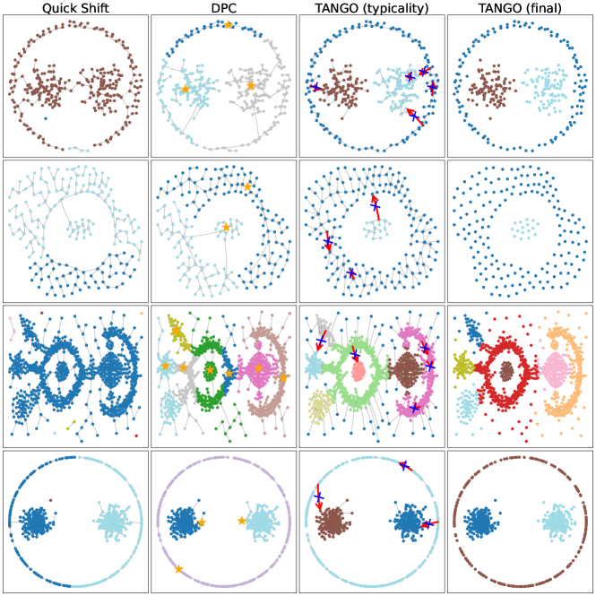
Figure 2: Results on 4 synthetic datasets. For TANGO, the hyperparameter $k$ is set to 20, 30, 70, and 30, respectively. For Quick Shift and DPC, we tune their hyperparameters to achieve a reasonable number of clusters while maximizing the Adjusted Rand Index (ARI).

Dataset	$n$	$d$	#Clusters
wdbc	569	30	2
heartEW	270	13	2
segmentation	2100	19	7
semeion	1593	256	10
semeionEW	1593	256	10
ver2	310	6	3
synthetic-control	600	60	6
waveform	5000	21	3
CongressEW	435	16	2
mfeat-zer	2000	47	10
ionosphereEW	351	34	2
banknote	1372	4	2
isolet1234	6238	617	26
Leukemia	72	3571	2
MNIST (AE)	10000	64	10
Umist (AE)	575	64	20

Table 1: Summary of real-world datasets.

Clustering on Real-word Datasets

We compared TANGO with 10 advanced algorithms based on density and local dependency relationships, as well as graph-cut clustering, on real-world datasets, including LDP-SC (Long et al. 2022), DCDP-ASC (Cheng et al. 2022), LDP-MST (Cheng et al. 2021), NDP-Kmeans (Cheng et al. 2023), DEMOS (Guan et al. 2023), CPF (Tobin and Zhang 2024), QKSPP (Jiang, Jang, and Kpotufe 2018), DPC-DBFN (Lotfi, Moradi, and Beigy 2020), USPEC (Huang et al. 2020), and KNN-SC (traditional spectral clustering based on $k$ nearest neighbor graph)

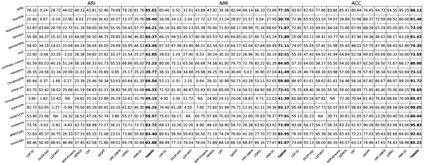
Figure 3: Results on $16$ real-world datasets (%, bold represents the best for a dataset).

We evaluated these algorithms using standard clustering metrics: Adjusted Rand Index (ARI; (Steinley 2004)), Normalized Mutual Information (NMI; (Xu, Liu, and Gong 2003)), and Accuracy (ACC; (Yang et al. 2010)).

For fair comparison, all algorithms were tuned to optimal hyperparameters. For TANGO, the neighborhood size $k$ was searched from 2 to 100 with a step size of 1. Algorithms requiring specification of the number of clusters used the ground-truth number of clusters. The detailed hyperparameter settings of the other algorithms are given in the supplementary material.

Experiments were conducted on 14 UCI datasets and 2 image datasets (Table 1). All datasets were min-max normalized. For image datasets MNIST and Umist, we used AutoEncoder (AE) to reconstruct them into 64-dimensional representations.

Fig. 3 presents the results of TANGO and 10 comparison algorithms on 16 real-world datasets. Specifically, LDP-MST on isolet1234 and NDP-Kmeans on ionosphereEW did not produce results due to the insufficient number of local density peaks compared to the target number of clusters. TANGO demonstrates superior performance across all datasets, by integrating local and global features of the data and employing a global graph-cut scheme.

Especially on datasets such as banknote, Leukemia, and MNIST (AE), TANGO outperforms other algorithms by a significant margin in various metrics. Algorithms based on local density peaks such as LDP-SC, DCDP-ASC, LDP-MST, NDP-Kmeans, and DEMOS performed poorly on multiple datasets, particularly DCDP-ASC and LDP-MST, which often yielded clustering results close to random division. This demonstrates the challenge of achieving satisfactory clustering results using only local data features. USPEC demonstrates strong clustering ability, ranking second after TANGO on multiple datasets, but it notably underperforms on datasets such as semeion and ver2 compared to TANGO. Moreover, USPEC requires extensive parameter tuning, limiting its practical utility.

Mode-seeking algorithms like CPF and QKSPP also exhibit significantly weaker performance compared to TANGO, highlighting the effectiveness of TANGO for removing incorrect connections through typicality and conducting global graph-cut.

We also obtained p $<0.05$ from Friedman’s test, and the pairwise mean rank differences between TANGO and other comparison algorithms surpassed the critical difference threshold (CD $=2.30$) in subsequent Nemenyi’s test, indicating the superior performance of TANGO is not due to random chance (see supplementary material).

Fig. 4 illustrates potentially incorrect dependency relationships identified by TANGO on the isolet1234 dataset (visualized in 2D using t-SNE for dimensionality reduction). The ability of TANGO to detect and remove such incorrect dependencies contributes to improved final clustering results.

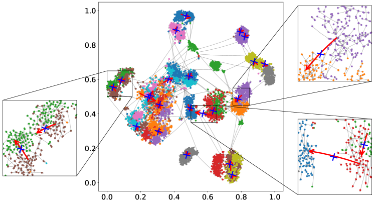
Figure 4: On the isolet1234 dataset, TANGO identified and severed potential incorrect associations.

Effects of the Hyperparameter $k$

The proposed TANGO algorithm has only one hyperparameter, which is the number of nearest neighbors $k$. Fig. 5 illustrates the performance of TANGO and three other density-based algorithms on six real-world datasets as the local neighborhood parameter $k$ varies. Here, the additional density fluctuation parameters of QKSPP and CPF are fixed at $0.7$ and $0.5$, respectively. From the figure, it is observed that the performance of TANGO tends to stabilize as $k$ increases and demonstrates strong overall effectiveness, whereas DPC-DBFN, QKSPP, and CPF exhibit significant fluctuations within the same parameter range. Moreover, in practical applications, optimizing the density fluctuation parameters of QKSPP and CPF requires fine-tuning to achieve optimal clustering results. Thus, TANGO demonstrates advantages in hyperparameter stability and practicability.

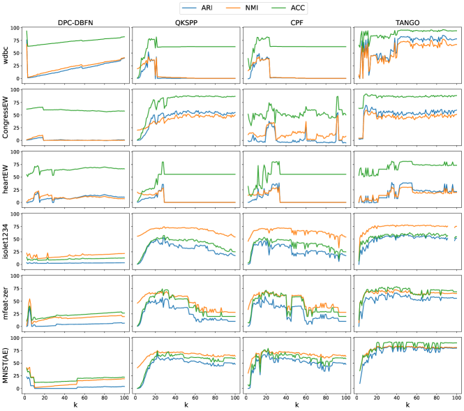
Figure 5: The impact of the number of neighbors $k$ on the performance of TANGO and other density-based algorithms.

Ablation Study

To validate the effectiveness of the main components of TANGO, we conducted ablation experiments by testing the performance after removing certain components:

• TANGO-a: Directly applying spectral clustering based on path-based similarity (Eq. (7)) to all data points.

• TANGO-b: Establishing dependency relationships without typicality, and applying spectral clustering on the sub-clusters using path-based similarity (Eq. (7)).

• TANGO-c: Replacing $C$ in Eq. (7) with the original similarity matrix $A$ to perform spectral clustering.

Fig. 6 illustrates the results of the ablation experiments. In nearly all datasets, the performance decreases when the corresponding component is removed, indicating that each component of the algorithm plays a significant role. Moreover, on some datasets like isolet1234, removing the typicality module (TANGO-b) results in a sharp decline in performance, highlighting the critical role of the typicality module.

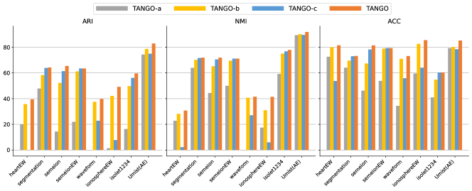
Figure 6: Results of ablation study.

Conclusion and Future Work

In this paper, we propose a novel clustering algorithm named TANGO to address the issues in current mode-seeking clustering algorithms. First, TANGO introduces the concept of typicality to identify and adjust potentially incorrect dependency relationships in a global perspective. Moreover, we establish constraining equations under rational postulates to calculate typicality, and theoretically show that a unique solution exists and can be found efficiently under dependency relationships given by density hierarchy. A global-view path-based similarity and graph-cut is then exploited to further partition the optimized sub-clusters by typicality, and to obtain final clustering results. Extensive experiments on multiple synthetic and $16$ real-world datasets demonstrate the effectiveness and superiority of TANGO over state-of-the-art clustering algorithms.

Future research could explore methods to automatically determine the hyperparameter $k$ and to investigate the effects of other types of dependency relationships on typicality.

References

- Altinigneli et al. (2020) Altinigneli, M. C.; Miklautz, L.; Böhm, C.; and Plant, C. 2020. Hierarchical Quick Shift Guided Recurrent Clustering. In ICDE, 1842–1845.
- Arias-Castro, Mason, and Pelletier (2016) Arias-Castro, E.; Mason, D.; and Pelletier, B. 2016. On the Estimation of the Gradient Lines of a Density and the Consistency of the Mean-Shift Algorithm. J. Mach. Learn. Res., 17: 43:1–43:28.
- Chang and Yeung (2008) Chang, H.; and Yeung, D. 2008. Robust path-based spectral clustering. Pattern Recognit., 41(1): 191–203.
- Cheng et al. (2023) Cheng, D.; Huang, J.; Zhang, S.; Xia, S.; Wang, G.; and Xie, J. 2023. K-Means Clustering With Natural Density Peaks for Discovering Arbitrary-Shaped Clusters. IEEE Transactions on Neural Networks and Learning Systems.
- Cheng et al. (2022) Cheng, D.; Huang, J.; Zhang, S.; Zhang, X.; and Luo, X. 2022. A Novel Approximate Spectral Clustering Algorithm With Dense Cores and Density Peaks. IEEE Trans. Syst. Man Cybern. Syst., 52(4): 2348–2360.
- Cheng, Zhang, and Huang (2020) Cheng, D.; Zhang, S.; and Huang, J. 2020. Dense members of local cores-based density peaks clustering algorithm. Knowl. Based Syst., 193: 105454.
- Cheng et al. (2021) Cheng, D.; Zhu, Q.; Huang, J.; Wu, Q.; and Yang, L. 2021. Clustering with Local Density Peaks-Based Minimum Spanning Tree. IEEE Trans. Knowl. Data Eng., 33(2): 374–387.
- Cheng (1995) Cheng, Y. 1995. Mean Shift, Mode Seeking, and Clustering. IEEE Trans. Pattern Anal. Mach. Intell., 17(8): 790–799.
- Du et al. (2018) Du, M.; Ding, S.; Xu, X.; and Xue, Y. 2018. Density peaks clustering using geodesic distances. Int. J. Mach. Learn. Cybern., 9(8): 1335–1349.
- Ester et al. (1996) Ester, M.; Kriegel, H.; Sander, J.; and Xu, X. 1996. A Density-Based Algorithm for Discovering Clusters in Large Spatial Databases with Noise. In KDD-96, 226–231.
- Fischer, Roth, and Buhmann (2003) Fischer, B.; Roth, V.; and Buhmann, J. M. 2003. Clustering with the Connectivity Kernel. In NeurIPS, 89–96.
- Guan et al. (2023) Guan, J.; Li, S.; Chen, X.; He, X.; and Chen, J. 2023. DEMOS: Clustering by Pruning a Density-Boosting Cluster Tree of Density Mounts. IEEE Trans. Knowl. Data Eng., 35(10): 10814–10830.
- Guan et al. (2021) Guan, J.; Li, S.; He, X.; Zhu, J.; and Chen, J. 2021. Fast hierarchical clustering of local density peaks via an association degree transfer method. Neurocomputing, 455: 401–418.
- Hartigan (1975) Hartigan, J. A. 1975. Clustering Algorithms. New York: Wiley.
- Huang et al. (2020) Huang, D.; Wang, C.; Wu, J.; Lai, J.; and Kwoh, C. 2020. Ultra-Scalable Spectral Clustering and Ensemble Clustering. IEEE Trans. Knowl. Data Eng., 32(6): 1212–1226.
- Jiang (2017) Jiang, H. 2017. On the Consistency of Quick Shift. In NeurIPS, 46–55.
- Jiang, Jang, and Kpotufe (2018) Jiang, H.; Jang, J.; and Kpotufe, S. 2018. Quickshift++: Provably Good Initializations for Sample-Based Mean Shift. In ICML, volume 80 of PMLR, 2299–2308.
- Jiang and Kpotufe (2017) Jiang, H.; and Kpotufe, S. 2017. Modal-set estimation with an application to clustering. In AISTATS, volume 54 of PMLR, 1197–1206.
- Katz (1953) Katz, L. 1953. A new status index derived from sociometric analysis. Psychometrika, 18: 39–43.
- Little, Maggioni, and Murphy (2020) Little, A. V.; Maggioni, M.; and Murphy, J. M. 2020. Path-Based Spectral Clustering: Guarantees, Robustness to Outliers, and Fast Algorithms. J. Mach. Learn. Res., 21: 6:1–6:66.
- Liu, Wang, and Yu (2018) Liu, R.; Wang, H.; and Yu, X. 2018. Shared-nearest-neighbor-based clustering by fast search and find of density peaks. Inf. Sci., 450: 200–226.
- Long et al. (2022) Long, Z.; Gao, Y.; Meng, H.; Yao, Y.; and Li, T. 2022. Clustering based on local density peaks and graph cut. Inf. Sci., 600: 263–286.
- Lotfi, Moradi, and Beigy (2020) Lotfi, A.; Moradi, P.; and Beigy, H. 2020. Density peaks clustering based on density backbone and fuzzy neighborhood. Pattern Recognit., 107: 107449.
- Ng, Jordan, and Weiss (2001) Ng, A. Y.; Jordan, M. I.; and Weiss, Y. 2001. On Spectral Clustering: Analysis and an algorithm. In NeurIPS, 849–856.
- Rodriguez and Laio (2014) Rodriguez, A.; and Laio, A. 2014. Clustering by fast search and find of density peaks. Science, 344(6191): 1492–1496.
- Steinley (2004) Steinley, D. 2004. Properties of the Hubert-Arable Adjusted Rand Index. Psychological Methods, 9(3): 386–396.
- Tobin and Zhang (2021) Tobin, J.; and Zhang, M. 2021. DCF: An Efficient and Robust Density-Based Clustering Method. In ICDM, 629–638.
- Tobin and Zhang (2024) Tobin, J.; and Zhang, M. 2024. A Theoretical Analysis of Density Peaks Clustering and the Component-Wise Peak-Finding Algorithm. IEEE Trans. Pattern Anal. Mach. Intell., 46(2): 1109–1120.
- Vedaldi and Soatto (2008) Vedaldi, A.; and Soatto, S. 2008. Quick Shift and Kernel Methods for Mode Seeking. In ECCV, volume 5305 of Lecture Notes in Computer Science, 705–718.
- Wang et al. (2023) Wang, Y.; Wang, D.; Zhou, Y.; Zhang, X.; and Quek, C. 2023. VDPC: Variational density peak clustering algorithm. Inf. Sci., 621: 627–651.
- Xu, Liu, and Gong (2003) Xu, W.; Liu, X.; and Gong, Y. 2003. Document clustering based on non-negative matrix factorization. In SIGIR, 267–273.
- Yang et al. (2010) Yang, Y.; Xu, D.; Nie, F.; Yan, S.; and Zhuang, Y. 2010. Image clustering using local discriminant models and global integration. IEEE Trans. Image Process, 19(10): 2761–2773.
- Zhan, Gurung, and Parsa (2017) Zhan, J.; Gurung, S.; and Parsa, S. P. K. 2017. Identification of top-K nodes in large networks using Katz centrality. J. Big Data, 4: 16.