Bayesian Uncertainty Quantification and Reliability Assessment for Mars Sample Return

Abstract

In this paper, we employ a Bayesian approach to assess the reliability of a critical component in the Mars Sample Return program, focusing on the Earth Entry System’s risk of containment not assured upon reentry. Our study uses Gaussian Process modeling under a Bayesian regime to analyze the Earth Entry System’s resilience against operational stress. This Bayesian framework allows for a detailed probabilistic evaluation of the risk of containment not assured, indicating the feasibility of meeting the mission’s stringent safety goal of $0.999999$ probability of success. The findings underscore the effectiveness of Bayesian methods for complex uncertainty quantification analyses of computer simulations, providing valuable insights for computational reliability analysis in a risk-averse setting.

Keywords: rare event, computer experiments, kriging

1 Introduction

In July 2020 the National Aeronautics and Space Administration (NASA) launched the Mars Perseverance Rover (Farley et al.,, 2020). Perseverance landed on Mars in February 2021 with the main goal of seeking signs of ancient life by the collection of rock cores, regolith and atmospheric samples for later evaluation on Earth (Beaty et al.,, 2019; Haltigin et al.,, 2022; Grady et al.,, 2022; Swindle et al.,, 2022; Carrier et al.,, 2022). Over the past several years, as Perseverance has been collecting samples, NASA and the European Space Agency (ESA) have been formulating the next elements of the Mars Sample Return (MSR) campaign. Prior to the re-architecture efforts undertaken in response to the second MSR Independent Review Board report (Figueroa et al.,, 2023), MSR would gather the sealed sample tubes, place them inside the Orbiting Sample (OS) container, launch them into Mars orbit, capture and contain them securely, and returm them safely to Earth through an Earth Entry System (EES) (Sarli et al.,, 2024).

In line with current policies (United Nations General Assembly,, 1967; COSPAR Panel on Planetary Protection,, 2021), the design, planning and execution of MSR must meet planetary protection requirements (NASA Office of Safety and Mission Assurance,, 2021, 2022). In this manuscript, we focus on Backward Planetary Protection (BPP), that is, protecting the Earth-Moon system from possible harmful extraterrestrial contamination that may be returned from Mars. These requirements translate into establishing and implementing a strategy and design concepts to break the chain of contact with Mars by isolating and robustly containing the restricted samples (Cataldo et al.,, 2024). To achieve compliance with these BPP requirements, quantitative targets have been established that correspond to a $0.999999$ probability of maintaining containment. Achieving this requires a statistical model involving both reliability analysis and extreme value distributions to assess the probability of a rare event, that is, the one-in-a-million probability of containment not assured, $\text{P}_{CNA}$. To evaluate the feasibility of this probabilistic goal, we focus on the assessment of the landing performance. In so doing, this paper specifically informs the process and prospects for complying with BPP policies using an EES-like vehicle.

In this analysis, we explore a particular cause of containment not assured when the maximum peak acceleration of the OS upon landing exceeds 3000 Gs. In particular, we examine the effects of uncertainty in specific materials properties of individual EES components. We note that while materials might react to additional unknowns affecting their behavior, this is beyond the scope of this paper. The uncertainty being used here is only due to the inherent variability of these materials properties. Assessing the reliability and $\text{P}_{CNA}$ of such complex systems involves significant uncertainty. Traditional deterministic methods may not be adequate to address such uncertainties due to inherent randomness and model parameter uncertainty. The Bayesian methodology, as a probabilistic approach, has been increasingly recognized as a powerful tool for managing uncertainty and variability in reliability analysis (Sankararaman and Mahadevan,, 2011, 2015). The aim of this study is to develop Bayesian methods that allow for model and parameter uncertainty as well as the inherent randomness of the system when assessing the probability of loss of containment.

In the following section, an overview of the data utilized is provided. In Section 3, we outline the methodology applied during our analysis. Section 4 is devoted to the application of these methods with respect to our specific data set as well as the results of the analysis. Section 5 provides a conclusion and recommendation for future work.

2 Data

For the use-case investigated here, earlier work completed by the Jet Propulsion Laboratory (JPL) identified 15 input variables comprising Young’s Modulus, Shear Modulus, and compressive and tensile strength in varying directions for two different materials, IM7 (a carbon fiber) and Kevlar (Carpenter,, 2021). Experimental tests executed by JPL provided initial observations for each of these 15 input variables. The number of observations for each variable ranges from 3 to 12. Previous Uncertainty Quantification (UQ) and reliability analysis work (Naresh et al.,, 2018; Fitt et al.,, 2019) as well as typical engineering practice suggest fitting two-parameter Weibull distributions to the strength variables and Normal distributions to the Modulus variables. Because of this precedence, as well as our small sample sizes and the need for extrapolation, we assume Weibull and Normal distributions, respectively. We use the indicators $X0001-X0015$ to identify the input variables moving forward and refer the reader to the supplementary materials for more details regarding the data.

After determining the parameters of the respective Normal and Weibull distributions for the 15 input variables using Maximum Likelihood Estimation (MLE), JPL engineers generated 25 samples of the input variables using Latin Hypercube Sampling (LHS). Using these 25 samples, the JPL engineers then ran 25 simulations of an LS-DYNA EES System-Level Impact Model (SLIM) and extracted peak OS acceleration as the quantity of interest (Livermore Software Technology, An Ansys Company,, 2021; Siddens et al.,, 2022, 2023). In the context of our analysis, we consider the 25 realization of peak OS acceleration as our output variable of interest. With the particulars of the data in mind, we next review the methods applied throughout our analysis.

3 Methods

In the following section, we outline the various methodologies employed in our analysis. A direct MLE approach is not appropriate because of the high dimension of the variable space and the low sample size; though we compare a functional regularized Restricted Maximum Likelihood (REML) approach to our preferred Bayesian method, which we favor due to its effective ability to incorporate uncertainty in the parameters. We begin with a consideration of the priors applied within the Bayesian analysis of our input variables.

3.1 Prior considerations

We have 15 input variables, each represented by either a Weibull or a Normal distribution; our goal with the Bayesian approach is to generate posterior distributions of the input variables’ parameters. For all the input variables, regardless of distributional assumptions, we compare the frequentist estimates provided by the MLE values and the mean of the posterior distributions generated by several priors within a Bayesian framework. That is, we assume a prior density on the unknown parameters $\pi_{0}(\psi)$ (here $\psi=(\alpha,\beta)$ or $\psi=(\mu,\sigma^{2})$ according to distributional assumption). Then, by applying Bayes’ Rule, we have $\pi(\psi\mid X_{1},\ldots,X_{n})=\frac{\pi_{0}(\psi)\prod_{i=1}^{n}{f(X_{i}\mid\psi)}}{\int\pi_{0}(\psi^{\prime})\prod_{i=1}^{n}{f(X_{i}\mid\psi^{\prime})}d\psi^{\prime}}$, where the distribution $\pi(\psi\mid X_{1},\ldots,X_{n})$ is known as the posterior distribution and reflects the updated knowledge of the parameters conditional on the data (Gelman et al.,, 2013).

The prior distribution is meant to reflect the prior knowledge one has in regard to the parameters. The degree of certainty surrounding these parameters can be controlled by the type of prior used in the analysis. The three priors we consider are a flat prior, which is non-informative, assigning equal probability to all parameter values; Jeffreys’ prior, which is also non-informative but scale-invariant and is defined by the square root of the determinant of the Fisher information matrix (Jeffreys,, 1939); and the conjugate prior, in which the prior and posterior distributions are part of the same probability family (Gelman et al.,, 2013) For the Weibull distribution we have an Inverse Gamma conjugate prior and for the Normal distribution, the Normal Inverse Gamma conjugate prior. While using certain priors, such as the conjugate prior, allows us to know the form of the posterior distribution, it is not always a straightforward task to generate a posterior distribution. In the next section, we discuss the use of an Adaptive Metropolis (AM) algorithm (Haario et al.,, 2001) that we implemented throughout our analysis in order to generate our posterior distributions.

3.2 Adaptive Metropolis (AM) algorithm

Once a prior distribution has been chosen, we look to generate values from the posterior distribution, $\pi(\bm{\psi}|X_{1}\ldots X_{n})$. One method of accomplishing this when the above distribution is intractable is by use of a Metropolis algorithm (Metropolis et al.,, 1953). This is an algorithm that can be used to obtain random samples from a probability distribution using a general symmetric proposal distribution where there is an associated accept/reject rate for the proposal distribution.

While this is a well-known, often-used algorithm, one issue typically cited is the difficulty in choosing a proposal distribution. The choice of proposal distribution greatly affects the speed of the algorithm and the acceptance probability, which is typically desired to be between $20-50\%$ (Gelman,, 1996). A feasible solution exists in the application of adaptive algorithms “which use the history of the process in order to ‘tune’ the proposal distribution suitably” (Haario et al.,, 2001). Haario et al., (2001) developed an AM algorithm that adapts continuously to the target distribution and is based on the original Metropolis algorithm (Metropolis et al.,, 1953) and its modifications as well as the Adaptive Proposal (AP) algorithm given in Haario et al., (1999).

The AP algorithm uses a Gaussian proposal distribution centered on the current state with the covariance calculated from a fixed finite number of previous states (Haario et al.,, 1999). The change to the AM algorithm is that the covariance of the proposal distribution is calculated using all the previous states (Haario et al.,, 2001). For further details on the specifics of the AM Algorithm and its implementation, we refer the reader to Haario et al., (2001).

Different variations of the Metropolis and Metropolis Hastings algorithms (Hastings,, 1970) were considered, such as the Delayed Rejection Adaptive Metropolis (DRAM) (Haario et al.,, 2006), the Hamiltonian Monte Carlo (Neal,, 2011), or the Metropolis-adjusted Langevin algorithm (MALA) (Roberts and Stramer,, 2002); however, for the balance in speed of computation and accuracy of algorithm results as well as the ease of implementation, we chose the AM algorithm. Another consideration in regards to the algorithm and its output was the number of iterations to apply and the amount of burn-in, if any, to remove. To make this determination, we relied on trace plots, running average plots, and the Geweke Convergence Diagnostic (GCD) (Geweke,, 1992). Now that we have discussed the AM algorithm, we turn our attention to the subjects of Gaussian processes and spatial statistics in relation to our modeling approach.

3.3 Gaussian processes and spatial statistics

First we consider the basic approach to modeling complex processes using computer simulations. Given a selection of input variables $\mathbf{X}=(X_{1},...,X_{k})$, an output variable, $Z=h(\mathbf{X})$, is produced by the computer code. In many instances, the goal of generating the output variable is prediction. Sacks et al., (1989) discusses the use of stochastic processes in modeling the prediction of the response variable while Kennedy and O’Hagan, (2001) expand upon this by using Bayesian methods in the calibration of computer models to improve the prediction process.

For our study, we model the output, $Z$, using a Gaussian Process (GP), a widely-used tool for dealing with spatially structured data (Rasmussen and Williams,, 2006). The GP provides a flexible, nonparametric approach, which is particularly apt at capturing spatial correlations (Cressie,, 1993). We define the GP model as $Z\sim N_{n}(X\beta,\Sigma)$, where Z represents the vector of simulation outputs, $X\beta$ denotes the mean response as a function of parameters $\beta$ ($X$ represents the design matrix of the GP, not the set of input variables previously defined as $\mathbf{X}$), and $\Sigma$ is the covariance matrix capturing the dependence structure among the data.

In GP s, the covariance between any two observations depends on the input locations corresponding to these observations. That is, we let $\Sigma=\alpha V(\mathbf{\theta})$, where $\alpha>0$ is a scale parameter and $V$ is a function of the spatial range parameters $\mathbf{\theta}$. Consistent with previous research (Sacks et al.,, 1989), $V$ is the squared exponential function. Assuming this form allows for an anisotropic covariance structure by using different spatial range parameters $\rho_{k}$, which scale the distances along each input dimension $k$, thus capturing varying influences of the inputs. We define $V$ by:

$$v_{ij}=\exp{\bigg{(}-\sum_{k=1}^{K}\frac{(s_{ik}-s_{jk})^{2}}{\rho_{k}^{2}}\bigg{)}}$$ (1)

where $s_{ik}$ and $s_{jk}$ are the $k$-th input variables of observations $i$ and $j$. We ensure the necessary positivity of the spatial range parameters for the Gaussian process model by setting $\theta_{k}=\log{\rho_{k}}$ (Rasmussen and Williams,, 2006).

To estimate our spatial range parameters, we again apply a Bayesian framework and compare those results to the MLE values. We consider several options using varying likelihood equations as outlined by Stein, (1999). We include some relevant equations as well as the likelihood equations in Table 1 but refer the interested reader to Stein’s book for further reference (Stein,, 1999).

Within our analysis we will employ the regularized REML Negative Log Likelihood (NLLH):

$$l_{R}(\theta)=l_{w}(\theta)+\lambda\sum_{k=1}^{K}(\theta_{k}-\bar{\theta})^{2}$$ (2)

for our MLE results. This particular formulation was incorporated in order to stabilize the estimation process which encountered issues due to the relatively small size of our data set. For the Bayesian portion of our analysis, we use the Bayesian NLLH:

$$l_{B}(\theta)=-\log{\pi(\theta)}+\frac{1}{2}\log{|V(\theta)|}+\frac{n-q}{2}\log{G^{2}(\theta)}+\frac{1}{2}\log{|X^{T}V(\theta)^{-1}X|}$$ (3)

where $\pi(\theta)$ is the prior distribution (Cressie,, 1993).

probability density function (pdf)	$f(Z|X\beta,\Sigma)=(2\pi)^{-\frac{n}{2}}|\Sigma|^{-\frac{1}{2}}\exp\left(-\frac{1}{2}[Z-X\beta]^{T}\Sigma^{-1}[Z-X\beta]\right)$
NLLH	$l(\beta,\alpha,\theta)=\frac{n}{2}\log(2\pi)+\frac{n}{2}\log(\alpha)+\frac{1}{2}\log{|V(\theta)|}+\frac{1}{2\alpha}[Z-X\beta]^{T}V(\theta)^{-1}[Z-X\beta]$
Estimates	$\hat{\beta}(\theta)=(X^{T}V(\theta)^{-1}X)^{-1}X^{T}V(\theta)^{-1}Z,\quad\hat{\alpha}(\theta)=\frac{G^{2}(\theta)}{n}$
Sub-expressions	$H=V(\theta)^{-1}-V(\theta)^{-1}X(X^{T}V(\theta)^{-1}X)^{-1}X^{T}V(\theta)^{-1},\quad G^{2}(\theta)=Z^{T}HZ$
Profile NLLH	$l_{p}(\theta)=l(\hat{\beta}(\theta),\hat{\alpha}(\theta),\theta)=\frac{n}{2}\log(2\pi)+\frac{n}{2}\log\left(\frac{G^{2}(\theta)}{n}\right)+\frac{1}{2}\log{|V(\theta)|}+\frac{n}{2}$
REML NLLH	$l_{w}(\theta)=\frac{n-q}{2}\log(2\pi)+\frac{n-q}{2}\log\left(\frac{G^{2}(\theta)}{n-q}\right)-\frac{1}{2}\log{|X^{T}X|}+\frac{1}{2}\log{|X^{T}V(\theta)^{-1}X|}+\frac{1}{2}\log{|V(\theta)|}+\frac{n-q}{2}$

Table 1: NLLH Equations

In the next section, we discuss the use of these varying methods, to include the Bayesian method with the prior $\theta_{1:K}\sim N(\tau,\nu^{2})$. We use Leave One Out Cross Validation (CV) twice, first to make an appropriate choice for the penalty term in the regularized REML case and again when choosing the hyperparameters $(\tau,\nu^{2})$ in the Bayesian case.

Once we have generated the posterior distributions for $\theta_{1:K}$, we can then predict new values from the computer simulations using a kriging approach. Kriging, a geostatistical interpolation technique, provides optimal, unbiased predictions by utilizing the spatial correlation structure inferred by the Gaussian process model (Cressie,, 1993; Stein,, 1999). We apply ordinary kriging to the problem, aiming to predict a new value $z_{0}$ with mean $x_{0}^{T}\beta$, variance $\sigma_{0}^{2}$, and covariance $\text{Cov}(z_{0},\mathbf{Z})=\phi$. We consider predictors of the form $\hat{z}_{0}=\gamma^{T}Z$ subject to the constraint $\gamma^{T}X=x_{0}^{T}$. Following the Lagrange Multiplier approach, we end up minimizing the mean squared prediction error (MSPE): $E[(z_{0}-\hat{z_{0}})^{2}]=\sigma_{0}^{2}-2\gamma^{T}\phi+\gamma^{T}\Sigma\gamma$ subject to the above constraint. Thus, our predictor and MSPE are:

$$\hat{z}_{0}=(x_{0}-X^{T}\Sigma\phi)\hat{\beta}+\phi^{T}\Sigma^{-1}\mathbf{Z}$$ (4)

$$E[(z_{0}-\hat{z_{0}})^{2}]=\sigma_{0}^{2}\phi^{T}\Sigma^{-1}\phi+(x_{0}-X^{T}\Sigma^{-1}\phi)^{T}(X^{T}\Sigma^{-1}X)^{-1}(x_{0}-X^{T}\Sigma^{-1}\phi)$$ (5)

After we have generated the posterior distributions for the parameters of the Normal and Weibull variables as well as for the spatial range parameters, we are able to predict the peak OS acceleration. A distinct advantage of the Bayesian approach to generate the spatial range parameters, as opposed to estimating the spatial process using MLE values for $\theta_{1:K}$, is that we are accounting for the error in the estimation of the spatial range parameters. This provides a more robust quantification of the underlying uncertainty within the model. With these elements in place, we can then simulate the posterior distribution of the probability of exceeding 3000 Gs with the given information.

3.4 Cross validation in a Bayesian setting

We mentioned in Section 3.3 that we would be using CV in two instances. In the first scenario, when choosing the penalty term for the regularized REML case, our CV follows the methods outlined by Hastie et al., (2009). For both uses of CV, we employ a squared error loss function. The algorithm used for the first CV is outlined in Algorithm 1. The input values for the algorithm are the input variables, $\mathbf{X}_{n\times K}$, the output variable, $\mathbf{Z}_{n\times 1}$, and the selected potential values for $\lambda$, $\mathbf{\Lambda}_{Q\times 1}$. The output of the algorithm is the vector of CV scores for each value of $\lambda$ used, $\mathbf{L}_{Q\times 1}$.

With the second use of CV, when choosing the hyperparameters in the Bayesian case, we follow the same methods but must account for the fact that we are dealing with posterior distributions of the $\theta_{k}$ values. In order to accommodate this addition, we adjust Algorithm 1 by applying the kriging step to every realization from the posteriors of $\theta_{1:K}$ (after removing burn-in) then calculate the squared error loss for each realization. Finally, we use the mean of the squared error loss across all of these realizations as the CV score for each potential set of hyperparameters. This update can be seen in Algorithm 2. We have the same input and output values as in Algorithm 1 except we use $\mathbf{P}_{Q\times 2}$ to represent the potential hyperparameter values instead of having a vector for the choice of $\lambda$. We also identify $T$ as the number of AM algorithm outputs and $b$ as the number of burn-in iterations removed.

Now that we have discussed all the elements that are used for generating the various posterior distributions, we move to the final step which is the simulation of the $\text{P}_{CNA}$.

Input: $\mathbf{X}_{n\times K}$, $\mathbf{Z}_{n\times 1}$, $\mathbf{\Lambda}_{Q\times 1}$, $n$, $Q$

Output: The set of CV values $\mathbf{L}_{Q\times 1}$ where $L_{q}=\sum_{i=1}^{n}(z_{0i}-\hat{z}_{0i}^{(q)})^{2}$

for $q\in 1,2,\ldots,Q$ do

       Set value of $\lambda$ from $\mathbf{\Lambda}$

       for $i\in 1,2,\ldots,n$ do

             Omit entry $i$ from $\mathbf{X}$ and $\mathbf{Z}$, set $n_{i}=n-1$ and $x_{0}$ as omitted vector from $\mathbf{X}$.

             Run optimization routine using Equation 2 to generate estimates for $\theta_{1:15}$.

             Perform kriging steps to generate $\hat{z}_{0i}^{(q)}$.

            

      Calculate $L_{q}=\sum_{i=1}^{n}(z_{0i}-\hat{z}_{0i}^{(q)})^{2}$

return Result: $\mathbf{L}_{Q\times 1}$

Algorithm 1 Cross Validation for Penalty Term $\lambda$

Input: $\mathbf{X}_{n\times K}$, $\mathbf{Z}_{n\times 1}$, $\mathbf{P}_{Q\times 2}$, $n$, $Q$, $T$, $b$

Output: The set of CV values $\mathbf{L}^{*}_{Q\times 1}$ where $L_{q}^{*}=\frac{1}{T-b}\sum_{j=1}^{T-b}L_{qj}$

for $q\in 1,2,\ldots,Q$ do

       Set value of $\tau$ and $\nu^{2}$ from $\mathbf{P}$

       for $i\in 1,2,\ldots,n$ do

             Omit entry $i$ from $\mathbf{X}$ and $\mathbf{Z}$, set $n_{i}=n-1$ and $x_{0}$ as omitted vector from $\mathbf{X}$.

             Run AM Algorithm using Equation 3 to generate posteriors: $\Theta_{15\times T}$.

             remove burn-in, $b$, from posterior results.

             for $j\in 1,2,\ldots,T-b$ do

                   Perform kriging steps to generate $\hat{z}_{0i_{j}}^{(q)}$.

                  

            

      for $j\in 1,2,\ldots,T-b$ do

             Calculate $L_{qj}=\sum_{i=1}^{n}(z_{0i}-\hat{z}_{0i_{j}}^{(q)})^{2}$

      Calculate $L^{*}_{q}=\frac{1}{T-b}\sum_{j=1}^{T-b}L_{qj}$

return Result: $\mathbf{L}^{*}_{Q\times 1}$

Algorithm 2 Cross Validation for Hyperparameters $\tau$ and $\nu^{2}$

3.5 Simulation of probability of containment not assured $(\text{P}_{CNA})$

Our end goal is to calculate the probability that the peak OS acceleration exceeds 3000 Gs, we will call this $z_{crit}$. In order to do this, we run a simulation based on Algorithm 3, fixing large $N$ and $M$. For each iteration of the simulation, we sample from the posterior distributions of parameters for our Weibull and Normal variables respectively in order to then generate a new set of input values $\mathbf{s}_{0}$. Additionally, we sample from the posterior distributions of the spatial range parameters, $\theta_{1:K}$ as input for the UQ model. Finally, we calculate the exceedance probability based on our previous GP assumption that $Z\sim N_{n}(X\beta,\Sigma)$. What results is a sample of probabilities that can be treated as the posterior distribution of the probability of exceeding 3000 Gs.

Input: Values: $N$, $M$, and $K$. Posterior distributions: $\pi(\alpha,\beta)$, $\pi(\mu,\sigma^{2})$, and $\pi(\theta_{k})$ for $k\in 1,\ldots,K$.

Output: The set of values $\hat{p}_{crit}^{(i)}$, $i=1,\ldots,N$, which is treated as a sample from the posterior distribution of $p_{crit}$.

for $i\in 1,2,\ldots,N$ do

       for $k\in 1,2,\ldots,K$ do

             Select values $\alpha_{k},\beta_{k},\mu_{k},\sigma_{k}$ from respective posterior distributions of the k^th input variable.

             Select values $\theta_{k}$ from the respective posterior distributions of the k^th spatial range parameter.

             These selections represent one sample from the posterior distribution.

            

      for $j\in 1,2,\ldots,M$ do

             for $k\in 1,2,\ldots,K$ do

                   Simulate one value of the Normal or Weibull distribution corresponding to the k^th input variable.This is our trial set of inputs $\mathbf{s}_{0}$.

                  

            Use the UQ model to obtain the mean predictor $\hat{z}_{0}$ and its RMSPE, $S_{0}$, at predictor $\mathbf{s}_{0}$.

             Calculate Exceedance probability: $1-\Phi(\frac{z_{crit}-\hat{z}_{0}}{S_{0}})$

      Average over $j=1,\ldots,M$ to obtain one estimate $\hat{p}_{crit}^{(i)}$ for the probability of exceeding $z_{crit}$.

      

return Result: $\hat{p}_{crit}^{(i)},i=1,\ldots,N$

Algorithm 3 $\text{P}_{CNA}$ Simulation

Having outlined the methodological framework and the statistical procedures used in this study, we now turn to the application of these methods. This includes applying our Gaussian process model and the associated kriging methodology to the data generated from the computer simulation. By employing the aforementioned techniques, we aim to illuminate the predictive capabilities of our model, demonstrating its practical relevance and validity. The following section thus presents the findings from this application, detailing the results and discussing their implications for our research question.

4 Application and Results

The overall analysis was completed in several steps, the first of which was to estimate the parameters for the Weibull and Normal distributions of the respective input variables. Next we estimated the spatial range parameters for the spatial model as well as evaluated the performance of our UQ model. Finally, we used Algorithm 3 to compute the distribution of the $\text{P}_{CNA}$.

4.1 Input variable analysis

Given the distributional assumptions on our 15 variables, we find the MLE values for $\mu$, $\sigma$ and $\alpha$, $\beta$, respectively; additionally, we apply the AM algorithm using all three of the aforementioned prior distributions (dependent on the distributional assumption). The MLE values give us an initial estimate on the parameters of the distributions. Allowing for different priors indicates how influential the choice of prior is on the posterior distribution. Additionally, when comparing the posterior means to the MLE values we can check the robustness of the results.

The results for the normally distributed variables can be seen in Figure 1 where the mean of the posterior distributions along with their 95% credible intervals (CIs) are plotted; additionally, the MLE s and their 95% confidence intervals are included for comparison. As observed in Figure 1(a), all the means and CIs are very similar. In Figure 1(b) we see less agreement in the scale parameter values, with some variation in the mean values as well as differing lengths of CIs; however, overall, the agreement across the priors is fairly consistent with no statistically significant differences.

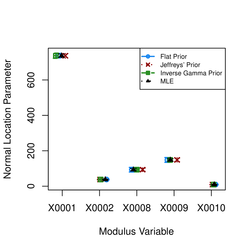
(a) Plot of posterior mean with 95% CIs for the location parameter of the Normally distributed variables.

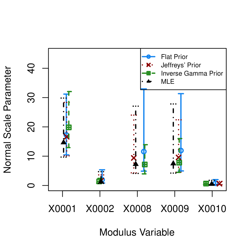
(b) Plot of posterior mean with 95% CIs for the scale parameter of the Normally distributed variables.

Figure 1: Posterior Distributions based on varying prior choices for the Normally distributed variables

Next we turn to the results for the Weibull distributed variables. Again we see plots of the mean and 95% CIs of the posterior distributions for the shape and scale parameters of the Weibull variables in Figure 2. Here we observe agreement for both the scale and shape parameters across prior choice. The consistency we see across prior choice in each instance demonstrates that the choice of prior is not overtaking the results; that is to say, the prior is not overly influential in the behavior of the posterior distributions.

Based on the results for both the Normal and Weibull variables, we use the posterior distributions that incorporated Jeffreys’ prior in further analysis steps. The main reasoning behind this is that Jeffreys’ prior gives more information than the flat prior (as it incorporates information about the structure of the model through the Fisher information) and does not have the extended parameter assumptions of a known shape parameter that is necessary when using a conjugate prior for the Weibull distribution.

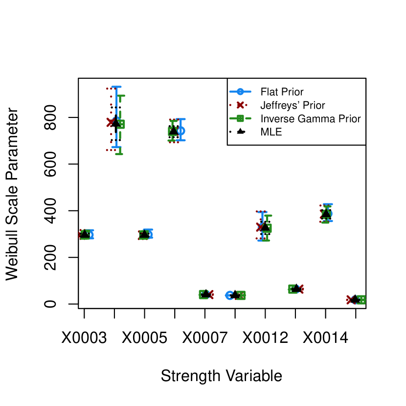
(a) Plot of posterior mean with 95% CIs for the scale parameter of the Weibull distributed variables.

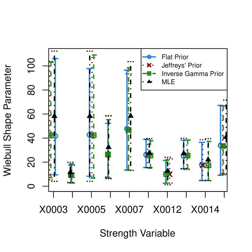
(b) Plot of posterior mean with 95% CIs for the shape parameter of the Weibull distributed variables.

Figure 2: Posterior Distributions based on varying prior choices for the Weibull distributed variables

4.2 Spatial range parameters analysis

Applying the GP approach to our data, we have $\mathbf{X}=(X0001,\ldots,X0015)$ as our input variables with the previously generated LHS as our input values for those variables. For our output variable $Z$, or the peak OS acceleration, we use the 25 realizations from JPL’s work. In our analysis, for numerical stability, we re-scaled the output data by dividing all output values by a factor of 1000, making our problem determining the probability that the peak OS acceleration is greater than $3.0$ when the input variables are random.

For simplicity, we assume a constant mean response for $X\beta$. Initially, we seek to determine the MLE values for the spatial range parameters $\theta_{1:K}$ with the overarching goal of generating posterior distributions for $\theta_{1:K}$ and then drawing from those distributions during the prediction (kriging) process. Considering several values of $\lambda>0$ via CV, we choose the value of $\lambda=2$ for our penalty term. We also completed the kriging step within the CV analysis at this point to see how our model performs in predicting the peak OS acceleration. The CV plot as well as a diagnostic plot of the model’s predictive quality can be seen in Figure 3.

From Figure 3, we see that $\lambda=2$ does provide the smallest CV value. In Figure 3 we see that the variance of the noise is greater than that of the signal. From this we consider that it is possible that the range of input values is too narrow; that is, we would get greater signal to noise ratio with a wider range of inputs. We also note that there are no simulated values in the critical region; that is, our $Z_{1:25}$ range from $2.474$ to $2.749$, so we have no data over $3.0$. Furthermore, kriging with a constant mean is a form of interpolation, which means it will never produce a predicted value outside the range of data and input values far from the test data set will simply be predicted back to the overall mean.

In spite of this critique, which we will discuss further in the next section, we move forward with the Bayesian analysis. We use Equation 3 with $\theta_{1:K}\sim N(\tau,\nu^{2})$ as the prior for the spatial range parameters; however, we must first determine appropriate values for $\tau$ and $\nu^{2}$. We start by using an Empirical Bayes approach, considering the MLE values of the Normal prior distribution for the $\theta_{i}$’s which are $\hat{\tau}=\bar{\theta}$ and $\hat{\nu}^{2}=\frac{1}{K}\sum_{i=1}^{K}{(\theta_{i}-\hat{\tau})^{2}}$. Here, as we do not have the actual values of $\theta_{1:K}$, we use the values generated from Equation 2 with $\lambda=2$ to calculate $\hat{\tau}$ and $\hat{\nu}^{2}$. However, when calculating $\hat{\nu}^{2}$ we get a value that is too small; that is, the MLE value of $\hat{\nu}^{2}$ suggests less variability than we believe truly exists. Therefore, we turn to the output of the Hessian matrix, $H$, from the optimization of Equation 2 and use $\hat{\nu}^{2}=\frac{1}{K}\sum_{i=1}^{K}{H_{i,i}^{-1}}$ as our estimate for $\nu^{2}$. This value provides a much more practical estimate of the variance at $0.259$ as compared to the MLE of $0.0364$.

(c) CV for regularized REML likelihood penalty term

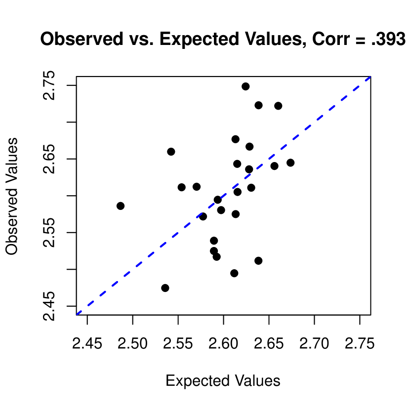
(d) Observed vs. Expected peak OS acceleration where observed are calculated using kriging methods described in Section 3.3

Figure 3: CV Results and Kriging Diagnostic Plot using Equation 2

After making the adjustment for $\hat{\nu}^{2}$, we then turn to CV to determine if the value of $\hat{\tau}=1.49$ as calculated from the output of optimizing Equation 2 is the best choice. In order to do this, for each potential value of $\tau$ under consideration, we run the adaptive algorithm $n=25$ times (as we used leave one out CV). Because of this, we narrowed the CV options to five potential values, $\tau=\{1.00,1.10,1.25,1.49,1.75\}$ based on some initial runs of the CV with fewer iterations for the AM algorithm. We see the results of the more extensive (in terms of number of iteration in the AM algorithm) CV analysis in Figure 4a which shows that $\hat{\tau}=1.25$ is the best option for our estimate of the mean of our prior distribution. To check the appropriateness of the choice for $\nu^{2}$, we did an additional round of CV with the same values of $\tau$ while using $\nu^{2}=0.5$. The CV scores with $\nu^{2}=0.5$ were consistently larger than when using $\nu^{2}=0.259$.

Once we determined the best choices for the hyperparameters of the prior distribution $(\tau=1.25,\nu^{2}=0.259)$, we examine the model performance using the chosen parameters. We also compare these results to those using the regularized REML approach with $\lambda=2$ as the penalty term. Comparing Figures 3 and 4, we see that the prediction using the Bayesian approach is slightly worse; however, this is to be expected given that we have allowed for more uncertainty within the choice of the spatial range parameters.

Finally, we examine the resulting values of the spatial range parameters from the Bayesian analysis. In Figure 5, we see the MLE results from Equation 2 plotted with their 95% confidence intervals as well as the posterior means and 95% CIs produced by the AM algorithm. As we can see, the two methods are fairly comparable, with the posterior mean estimates from the Bayesian method pooling toward the common mean, driven by the choice of $\tau=1.25$ as the mean of the prior distribution. This regularization in the Bayesian context is to be expected given the few number of data points we have, making the influence of the prior stronger.

(a) CV for regularized REML likelihood penalty term

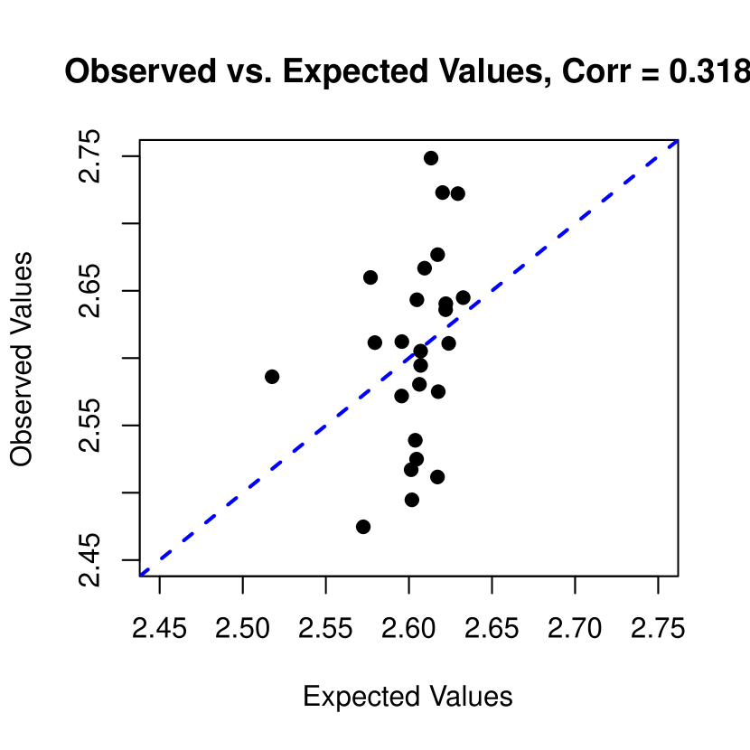
(b) Observed vs. Expected peak OS acceleration where observed are calculated using kriging methods described in Section 3.3

Figure 4: CV Results for Spatial Range Parameters and Kriging Diagnostic Plot using Equation 3

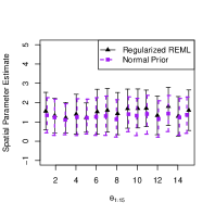
Figure 5: Comparison of MLE and Bayesian results

Now that we have posterior distributions for all of the parameters of our Normal and Weibull variables $(X0001,\ldots,X0015)$ as well as our spatial range parameters $(\theta_{1:15})$, we can move forward with our end-to-end analysis.

4.3 Final simulation results

We run the end-to-end simulation found in Algorithm 3 using two settings. In both settings A and B, we use the posterior distributions for $\alpha,\beta,\mu,\sigma^{2}$ generated by applying the AM algorithm with the respective Jeffreys’ priors. For the spatial range parameters $\theta_{1:15}$ in Setting A, we use the MLE results given by Equation 2 with penalty term $\lambda=2$. And in Setting B, for the spatial range parameters $\theta_{1:15}$ we use the posteriors produced by applying the AM algorithm with Equation 3 and prior $\theta_{k}\sim N(1.25,0.259)$. In both settings, we let $N=2000$ and $M=1000$. The resulting posterior distributions of the $\text{P}_{CNA}$ can be seen in Figure 6.

As observed in Figure 6a under Setting A, both the median and mean of the posterior distribution fail to meet the target value of one, or the probability of one in a million. However, in Figure 6b, the median of the posterior is well below the target value at $0.13$ and the mean only slightly exceeds the target value at $1.16$. We also see a narrower credible interval under Setting B. Thus, even though we have included a greater amount of uncertainty by varying the values of the spatial range parameters in Setting B, the $\text{P}_{CNA}$ appears to be reduced. A deeper dive into this result concluded that this change is due to the slight decrease in the spatial range parameter estimates and is specifically tied to the choice of prior parameters.

While this raises some concerns, we emphasize the extensive exploration in selecting the parameter values of the prior via CV. That is, in the context of this problem, we have incorporated empirical evidence by beginning with the MLE values for the spatial range parameters and then applying CV to choose hyperparameter values for the prior on the spatial range parameters in the Bayesian framework. Although the variability in $\theta_{1:K}$ has a strong influence on the final $\text{P}_{CNA}$ distribution, we have built some assurance in the results in Figure 6b with the systematic approaches outlined above. The implications of these findings and potential avenues for future research are discussed in the following section.

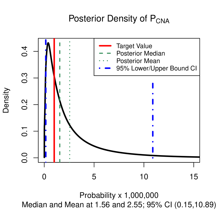
(a) Plot of posterior distribution of the $\text{P}_{CNA}$ under Setting A

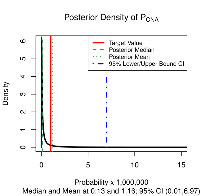
(b) Plot of posterior distribution of the $\text{P}_{CNA}$ under Setting B

Figure 6: Comparison of Posterior Distributions of $\text{P}_{CNA}$ between settings A and B

5 Conclusion and Future Work

The general process outlined and applied above gives a Bayesian approach to UQ of computer simulations. In context of the overarching goal for the MSR program, we have demonstrated a model for providing a measurement of the $\text{P}_{CNA}$ for the EES. By employing Bayesian methods, we produce a probability density of the $\text{P}_{CNA}$ as opposed to a singular point estimate. While our method and the subsequent results have limitations, we have ascertained that the predominant goal of ensuring containment at least equal to $99.9999\%$ is conceivable for this particular component. Additionally, providing decision makers with CIs allows for further risk assessment and analysis in the event that the stated goal has some flexibility. Indeed, these results would be factored into larger reliability analyses (Cataldo et al., nd, ) as part of the assurance case MSR is developing per NASA’s requirements (NASA Office of Safety and Mission Assurance,, 2021).

Several of the limitations within this analysis suggest directions for future projects. The first was mentioned in Section 4.2 in regard to kriging with a constant mean. While this element of the model could be modified, we believe the real issue here is the data used to generate the initial set of output values. We mentioned the engineers running the experiment used LHS when sampling from the input variables. This is a perfectly valid method of sampling as outlined by McKay et al., (1979). However, the 25 LHS samples fail to produce an example of the peak OS acceleration exceeding 3000 Gs when run through the chosen computer model. Therefore, we ask, if the simulation does not produce a critical value, how can we understand the conditions under which a critical value might occur in reality? To avoid this issue, we suggest a study on the comparison of sampling methods in respect to their impact on the $\text{P}_{CNA}$.

Although we believe that our method effectively exploits the data that are available, we also believe it highlights the disadvantages of working with such a limited dataset. As the initial computer model only produced 25 simulations of the peak OS acceleration, we were very limited in testing the robustness of our UQ model. There were multiple reasons for the number of runs conducted by JPL which include the cost of experiments as well as the length of time the simulation software takes. However, given the work we have done here, our counterparts at JPL have been receptive to the following suggestion. We propose the engineers generate more simulations using their computer model, perhaps using a sampling scheme as indicated by our next planned study. This would allow us to reapply the methods used in this paper and explore further alternative techniques if we meet the same sensitivity issues in regards to the influence of the choice of spatial range parameters in the GP model.

Finally, we outlined the chain of influence the choice of the spatial range parameters has on the final probability distribution. To explore this influence further, the future study with the incorporation of additional data should consider alterations to the model. These alterations would include examining a change to the GP’s covariance structure, and/or a change to the GP’s mean function, as well as a larger scale change in the distributional assumptions for the output variable $Z$ (e.g., a t-distribution). Exploring these different avenues, bolstered by additional data, will allow us to hone our methodology within this particular problem set and strengthen our abilities to apply such methods to additional aspects of the MSR program.

In conclusion, our work shines a light on the significant potential of the Bayesian approach in UQ for computer simulations, particularly in the context of complex projects such as the MSR. The highlighted limitations and subsequent recommendations not only provide a road map for immediate improvements but also emphasize the interdisciplinary nature of this research, bridging the gap between statistical methodologies and engineering challenges. As we advance further into an era dominated by simulations and computational models, understanding the underpinnings of their uncertainties becomes paramount. As we move forward, augmenting our dataset and refining our methodologies will be instrumental in enhancing the reliability and precision of our computational assessments.

Supplementary Materials

In the supplementary materials we define the settings we used when applying the AM algorithm. We also include information on hyperparameter choices and further algorithm settings when using CV for the spatial range parameters. In separate files, we include the data and code.

Disclosure Statement

The authors report there are no competing interests to declare.

SUPPLEMENTARY MATERIAL

Data:

The description of the different variables as well as the number of observations and the distributional assumptions can be seen in Table 2.

Indicator	Parameter	Description	Num of Obs	Distributional Assumption
X0001	$IM7-E_{a},E_{b},E_{c}$	Young’s Modulus	8	Normal
X0002	$IM7-G_{ab},G_{bc},G_{ca}$	Shear Modulus	4	Normal
X0003	$IM7-X_{c}$	Compressive Strength (0 Deg)	3	Weibull
X0004	$IM7-X_{t}$	Tensile Strength (0 Deg)	4	Weibull
X0005	$IM7-Y_{c}$	Compressive Strength (90 Deg)	3	Weibull
X0006	$IM7-Y_{t}$	Tensile Strength (90 Deg)	4	Weibull
X0007	$IM7-S_{c}$	Shear Strength	4	Weibull
X0008	$Kv-E_{a},E_{c}$	Young’s Modulus (0 Deg)	4	Normal
X0009	$Kv-E_{b}$	Young’s Modulus (90 Deg)	4	Normal
X0010	$Kv-G_{ab},G_{bc},G_{ca}$	Shear Modulus	4	Normal
X0011	$Kv-X_{c}$	Compressive Strength (0 Deg)	12	Weibull
X0012	$Kv-X_{t}$	Tensile Strength (0 Deg)	4	Weibull
X0013	$Kv-Y_{c}$	Compressive Strength (90 Deg)	11	Weibull
X0014	$Kv-Y_{t}$	Tensile Strength (90 Deg)	4	Weibull
X0015	$Kv-S_{c}$	Shear Strength	4	Weibull

Table 2: Description of input variables

AM algorithm settings:

We refer the reader to Haario et al., (2001) for an in-depth description of the AM algorithm. For every application of the AM algorithm unless otherwise noted, we set the total number of simulations to: $t=100,000$; we also set the following values: $s_{d}=\frac{(2.4)^{2}}{d}$ ($d$ is the dimension of the sample parameter space), $\epsilon=0.0001$, $t_{0}=10,000$ ($t_{0}$ is the length of the initial period (Haario et al.,, 2001), $t_{1}=10$ ($t_{1}$ is length of iterations between updating the covariance matrix), as well as $t_{2}=100$ ($t_{2}$ is the interval between updates of our output parameter matrix). Therefore, we end up with an output parameter matrix of dimension $\frac{t}{t_{2}}\times d=1,000\times d$. The number of total simulations was chosen after some initial runs at varying values; the choice of $t=100,000$ was based on the trace plots and running average plots. The values for $t_{0},t_{1}$, and $t_{2}$ were based on the speed of the algorithm as well as our confidence in the initial covariance matrix (in regards to $t_{0}$). After establishing the above settings of the AM algorithm, we looked at trace plots and running average plots as well as the GCD for each application of the AM algorithm in order to assess the burn-in rate for the algorithm. Taking into consideration all of these diagnostics, we removed the first 20% of the runs as burn-in for each use of the AM algorithm unless otherwise specified.

Hyperparameter choices for input variables:

For the Normally distributed variables, the hyperparameters for the Normal Inverse Gamma (NIG) were tuned and set to $m=10$, $c=0.003$, $a=0.1$, and $b=0.5$. And for the Weibull variables, the hyperparameters for the Inverse Gamma (IG) prior were tuned and set the hyperparameters to $\gamma=1,\zeta=2$.

Spatial range parameter CV:

We performed the CV using the following two settings for the AM algorithm, Setting 1: $t=5,000,t_{0}=500,t_{1}=10,t_{2}=50$ and Setting 2: $t=10,000,t_{0}=1,000,t_{1}=10,t_{2}=100$. We did not increase the total number of iterations to $100,000$ due to the projected length of time the CV would take. In both CV runs with the above settings, the conclusions agreed with the results presented in the body of the paper.

References

- Beaty et al., (2019) Beaty, D. W. et al. (2019). The Potential Science and Engineering Value of Samples Delivered to Earth by Mars Sample Return. Meteoritics and Planetary Science, 54(3):667–671.
- Carpenter, (2021) Carpenter, K. (2021). Uncertainty quantification for the eev energy absorber: Proof of concept. JPL Internal Memo.
- Carrier et al., (2022) Carrier, B. L. et al. (2022). Science and Curation Considerations for the Design of a Mars Sample Return (MSR) Sample Receiving Facility (SRF). Astrobiology, 22(S1):S–217–S–237. PMID: 34904886.
- Cataldo et al., (2024) Cataldo, G. et al. (2024). The Planetary Protection Strategy of Mars Sample Return’s Earth Return Orbiter Mission. Journal of Space Safety Engineering, Accepted.
- (5) Cataldo, G., Grello, Braverman, and Gage (n.d.). Reliability analyses and risk assessments for mars sample return. In preparation.
- COSPAR Panel on Planetary Protection, (2021) COSPAR Panel on Planetary Protection (2021). COSPAR Policy on Planetary Protection. Space Research Today, 211:12–25.
- Cressie, (1993) Cressie, N. A. C. (1993). Statistics for Spatial Data. John Wiley and Sons.
- Farley et al., (2020) Farley, K. A. et al. (2020). Mars 2020 Mission Overview. Space Science Reviews, 216(142).
- Figueroa et al., (2023) Figueroa, O., Kearns, S., Boll, N., and Elbel, J. (2023). Mars Sample Return (MSR) Independent Review Board-2 Final Report. Accessed: 21 May 2024.
- Fitt et al., (2019) Fitt, D., Wyatt, H., Woolley, T. E., and Mihai, L. A. (2019). Uncertainty quantification of elastic material responses: testing, stochastic calibration and bayesian model selection. Mechanics of Soft Materials, 1.
- Gelman, (1996) Gelman, A. (1996). Efficient metropolis jumping rules. Bayesian statistics, 5:599–607.
- Gelman et al., (2013) Gelman, A., Carlin, J. B., Stern, H. S., Dunson, D. B., Vehtari, A., and Rubin, D. B. (2013). Bayesian Data Analysis. CRC Press, 3 edition.
- Geweke, (1992) Geweke, J. (1992). Evaluating the accuracy of sampling-based approaches to calculating posterior moments. Bayesian Statistics, 4:169–193.
- Grady et al., (2022) Grady, M. M. et al. (2022). The Scientific Importance of Returning Airfall Dust as a Part of Mars Sample Return (MSR). Astrobiology, 22(S1):S–176–S–185. PMID: 34904884.
- Haario et al., (2006) Haario, H., Laine, M., Mira, A., and Saksman, E. (2006). Dram: Efficient adaptive mcmc. Statistics and Computing, 16(4):339–354.
- Haario et al., (1999) Haario, H., Saksman, E., and Tamminen, J. (1999). Adaptive proposal distribution for random walk metropolis algorithm. Computational Statistics, 14(3):375–395.
- Haario et al., (2001) Haario, H., Saksman, E., and Tamminen, J. (2001). An adaptive metropolis algorithm. Bernoulli, 7(2):223–242.
- Haltigin et al., (2022) Haltigin, T. et al. (2022). Rationale and Proposed Design for a Mars Sample Return (MSR) Science Program. Astrobiology, 22(S1):S–27–S–56. PMID: 34904885.
- Hastie et al., (2009) Hastie, T., Tibshirani, R., and Friedman, J. (2009). The Elements of Statistical Learning: Data Mining, Inference, and Prediction. Springer, 2nd edition.
- Hastings, (1970) Hastings, W. (1970). Monte carlo sampling methods using markov chains and their applications. Biometrika, 57(1):97–109.
- Jeffreys, (1939) Jeffreys, H. (1939). Theory of Probability. Oxford University Press, Oxford.
- Kennedy and O’Hagan, (2001) Kennedy, M. C. and O’Hagan, A. (2001). Bayesian calibration of computer models. Journal of the Royal Statistical Society: Series B (Statistical Methodology), 63(3):425–464.
- Livermore Software Technology, An Ansys Company, (2021) Livermore Software Technology, An Ansys Company (2021). LS-DYNA Keyword User’s Manual, Version R13. Accessed January 30, 2024.
- McKay et al., (1979) McKay, M. D., Beckman, R. J., and Conover, W. J. (1979). A comparison of three methods for selecting values of input variables in the analysis of output from a computer code. Technometrics, 21(2):239–245.
- Metropolis et al., (1953) Metropolis, N., Rosenbluth, A. W., Rosenbluth, M. N., Teller, A. H., and Teller, E. (1953). Equation of state calculations by fast computing machines. The Journal of Chemical Physics, 21(6):1087–1092.
- Naresh et al., (2018) Naresh, K., Shankar, K., and Velmurugan, R. (2018). Reliability analysis of tensile strengths using weibull distribution in glass/epoxy and carbon/epoxy composites. Composites Part B: Engineering, 133:129–144.
- NASA Office of Safety and Mission Assurance, (2021) NASA Office of Safety and Mission Assurance (2021). Planetary Protection Provisions for Robotic Extraterrestrial Missions. NASA Procedural Requirements (NPR) 8715.24.
- NASA Office of Safety and Mission Assurance, (2022) NASA Office of Safety and Mission Assurance (2022). Implementing planetary protection requirements for space flight. NASA Technical Standard 8719.27, NASA.
- Neal, (2011) Neal, R. M. (2011). Mcmc using hamiltonian dynamics. In Handbook of Markov Chain Monte Carlo. Chapman and Hall, CRC Press.
- Rasmussen and Williams, (2006) Rasmussen, C. E. and Williams, C. K. I. (2006). Gaussian Processes for Machine Learning. The MIT Press.
- Roberts and Stramer, (2002) Roberts, G. O. and Stramer, O. (2002). Langevin diffusions and metropolis-hastings algorithms. Methodology and Computing in Applied Probability, 4(4):337–358.
- Sacks et al., (1989) Sacks, J., Welch, W. J., Mitchell, T. J., and Wynn, H. P. (1989). Design and analysis of computer experiments. Statistical Science, 4(4):409–423.
- Sankararaman and Mahadevan, (2011) Sankararaman, S. and Mahadevan, S. (2011). Model validation under epistemic uncertainty. Reliability Engineering and System Safety, 96(9):1232–1241. Quantification of Margins and Uncertainties.
- Sankararaman and Mahadevan, (2015) Sankararaman, S. and Mahadevan, S. (2015). Integration of model verification, validation, and calibration for uncertainty quantification in engineering systems. Reliability Engineering and System Safety, 138:194–209.
- Sarli et al., (2024) Sarli, B. V. et al. (2024). NASA Capture, Containment, and Return System: Bringing Mars Samples to Earth. Acta Astronautica,, Accepted.
- Siddens et al., (2023) Siddens, A., Pempejian, J., Coleman, D., Vena, M., Yu, M., and Costain, A. (2023). Impact Testing for Model Validation and Hardware Verification for Mars Sample Return Landing Phase. In 20th International Planetary Probe Workshop, Marseille, France, Aug 28-Sept 1.
- Siddens et al., (2022) Siddens, A., Perino, S., and Sprunt, A. (2022). Earth Landing Loads for the Mars Sample Return Earth Entry System. In 2022 Spacecraft Launch Vehicle Dynamic Environments Workshop, June 28-30.
- Stein, (1999) Stein, M. L. (1999). Interpolation of Spatial Data: Some Theory for Kriging. Springer.
- Swindle et al., (2022) Swindle, T. D. et al. (2022). Scientific Value of Including an Atmospheric Sample as Part of Mars Sample Return (MSR). Astrobiology, 22(S1):S–165–S–175. PMID: 34904893.
- United Nations General Assembly, (1967) United Nations General Assembly (1967). 2222 (XXI). Treaty on Principles Governing the Activities of States in the Exploration and Use of Outer Space, including the Moon and Other Celestial Bodies. Article IX.