On the flux density spectral property of high linearly polarized signal from Pulsar J0332+5434

Abstract

The polarization position angles (PPA) of time samples with high linear polarization often show two parallel tracks across the pulsar profile that follow the rotating vector model (RVM). This feature support coherent curvature radiation (CCR) as the underlying mechanism of radio emission from pulsars, where the parallel tracks of the PPA represent the orthogonal extraordinary X and ordinary O eigen modes of strongly magnetized pair plasma. However, the frequency evolution of these high linearly polarized signals remains unexplored. In this work we explore the flux density spectral nature of high linearly polarized signals by studying the emission from PSR J0332+5434 over a frequency range between 300 MHz and 750 MHz, using the Giant Metrewave Radio Telescope. The pulsar average profile comprises of a central core and a pair of conal components. We find the high linearly polarized time samples to be broadband in nature and in many cases they resemble a narrow spiky feature in the conal regions. These spiky features are localised within a narrow pulse longitude, over the entire frequency range, and their spectral shapes sometimes resemble an inverted parabolic shape. In all such cases the PPA are exclusively along one of the orthogonal RVM tracks, likely corresponding to the X-mode. The inverted spectral shape can in principle be explained if the high linearly polarized emission in these time samples are formed due to incoherent addition of CCR from a large number of charged solitons (charge bunches) exciting the X-mode.

1 Introduction

PSR J0332+5434 (B0329+54) discovered in 1968 (Cole & Pilkington, 1968) is one of the brightest pulsars in the northern sky and as a result has been extensively studied over the radio spectrum from about 25 MHz to 43 GHz. Over a majority of this frequency range the pulsar profiles have three distinct emission components, consisting of a dominant central core surrounded by a pair of leading and trailing conal components, but the profiles are scattered by the inter stellar medium (ISM) below 100 MHz. The core component has a composite nature and becomes comparatively weaker with increasing frequency (see e.g. Shang et al., 2017; Basu et al., 2021). The profile type has been classified as core-outer cone triple (Rankin, 1993a, b), although some studies also reported the presence of additional inner cones (Gangadhara & Gupta, 2001). The pulsar profile shows the effect of radius to frequency mapping where the profile width progressively decreases at higher frequencies (Mitra & Rankin, 2002). The pulsar exhibits moderate levels of average linear and circular polarization across frequencies. The average polarization position angle (PPA) has a complex traverse across the profile, but single pulse observations have revealed two parallel PPA tracks (Gil & Lyne, 1995; Mitra et al., 2007) that follow the rotating vector model (Radhakrishnan & Cooke, 1969, hereafter RVM). According to RVM the linearly polarized emission traces the change in the dipolar magnetic field line plane of the rotating pulsar, and the model has been extensively used to measure the location of the radio emission region and emission geometry in several pulsars (see Mitra, 2017; Mitra et al., 2024, for a review).

The average flux density spectra in pulsars generally exhibit a steep power law nature ($S\propto\nu^{\alpha}$) above 100 MHz with typical spectral indices, $\alpha\sim-1.8$ (Maron et al., 2000; Jankowski et al., 2018). However, the spectrum of PSR J0332+5434 deviates from this typical behaviour and can be approximated as a broken power law, where at the high frequency range above 1 GHz the spectrum is steeper, while between 100 MHz and 1 GHz it becomes much flatter. The flux densities in pulsars usually show large fluctuations due to variations in the parameter of emission mechanism as well as scintillations during propagation in the ISM. As a result the spectral measurement requires averaging the flux density over longer timescales, usually several thousand pulses, to obtain a stable value. One of the drawbacks of the flux density estimates is that in the averaging process the information of the individual emission sources in the pulsar plasma, which last for significantly shorter timescales, is wiped out. Hence, our understanding of the coherent radio emission mechanism produced by these individual emission can benefit from the study of single pulse spectra across frequencies. The initial attempt at characterising the single pulse spectra was conducted by Kramer et al. (2003, hereafter K03), who carried out simultaneous observations of two pulsars, J0332+5434 and J1136+1551, over a wide frequency range between 200 MHz and 5 GHz. Their study showed that the single pulse flux densities have stronger correlation between nearby frequencies and the correlation gets weaker when widely separated frequencies are considered. This behaviour indicates that the radiation source in pulsars influences the single pulse spectra and motivates this present work of using single pulse spectral properties to study the underlying emission process.

In PSR J0332+5434, K03 found the spectra of the single pulses to be similar to the average spectrum, suggesting the possibility of a relatively stable and unvarying emission process on shorter timescales, although this does not provide any further constraints on the underlying emission mechanism. Recent studies have uncovered that PPAs of high linearly polarized time samples in single pulses are oriented along two parallel tracks, separated by 90$\arcdeg$ in phase, that closely follow the RVM, even in pulsars where the average PPA shows complex non-RVM like PPA traverse (Mitra et al., 2023a, b; Johnston et al., 2024). The feature that the high linearly polarized time sample follow the RVM can be only explained by curvature radiation, since the waves excited by curvature radiation are polarized parallel or perpendicular to the curved magnetic field line planes (see Mitra et al. 2024 for a recent review). Further the requirement of high brightness temperature of the pulsar radio emission establishes coherent curvature radiation (CCR) from charged bunches as the most likely emission mechanism. The high linearly polarized signals are free from depolarization and correspond exclusively to a single polarization state. The two orthogonal polarization states of the PPA can be associated with the extraordinary (X) and ordinary (O) eigen modes of a strongly magnetized pair plasma excited by CCR, with the polarization vector oriented perpendicular and parallel to the magnetic field line planes, respectively. Hence, it is expected that the spectra of these high linearly polarized time samples should provide additional constraints on the emission mechanism by bearing resemblance to the CCR spectra of individual charged bunches.

In this paper we explore the spectral nature of high linearly polarized time samples by carrying out simultaneous observations of single pulse polarization from PSR J0332+5434 over a frequency range, between 300 MHz and 750 MHz, using the Giant Meterwave Radio Telescope (GMRT,Swarup et al. 1991). We intend to examine whether these highly polarized time samples are broadband in nature and find their spectral behaviour over the observed frequency range. In section 2 we describe the observations and data analysis methods. Section 3 reports the spectral properties of the high linearly polarized time samples while section 4 provides a qualitative understanding of the spectra from the perspective of CCR from charge bunches. In section 5 we summarize the spectral nature of the highly polarized time samples of PSR J0332+5434.

2 Observation & Analysis

A group of bright pulsars, including PSR J0332+5434, were observed using the GMRT between December 2019 and February 2020. The GMRT is an interferometer consisting of 30 antennas, each of 45 meter diameter, and upgraded wideband receiver systems (Gupta et al., 2017) operating at four distinct frequency bands between 120-250 MHz (Band2), 250-500 MHz (Band-3), 550-850 MHz (Band-4), and 1050-1450 MHz (Band-5). The antennas are arranged resembling a Y-shaped array with two distinct configurations, a central square populated by 14 antennas spread within an area of 1 square km, and 16 antennas along three arms within a circle of 25 km diameter. The high time resolution observations for studying pulsars usually employs the phased-array mode where the signals from different antennas are co-added in phase. However, accurate flux density measurements require interferometric imaging. The GMRT allows the simultaneous measurements in both phased-array and interferometric modes.

The whole array can be divided into several subarrays, with different sets of antennas, observing simultaneously at multiple frequency bands. PSR J0332+5434 was observed on 17 January 2020 using dual subarrays at Band-3 and Band-4, with 200 MHz bandwidth, such that the pulsar emission could be recorded with a near continuous frequency coverage between 300 MHz and 750 MHz. During this session a total of 26 antennas were available for observations, with 3 antennas from the central square and 1 from an arm affected by technical issues. The first subarray in Band-3 (300-500 MHz) had 9 antennas, comprising of 6 central square antennas and 3 arm antennas, while the remaining 17 antennas were observing in Band-4 (550-750 MHz), comprising of 5 central square antennas and 12 arm antennas. The phased array used the central square antennas and the first two arm antennas while all available antennas in each subarray were part of the interferometric measurements. More central square antennas were part of the Band-3 subarray as the de-phasing of the nearby antennas would be slower allowing longer scans for single pulse studies. All four polarizations in the full Stokes mode were measured during these observations with the 200 MHz band divided into 2048 spectral channels. The entire 400 MHz frequency range was further subdivided into 6 subbands of 50-60 MHz (see Table 1), after removing channels affected by Radio frequency Interference (RFI), to study the spectral nature of the emission. The output signals from the phased array, that can be considered equivalent to a single dish, were sampled at high temporal resolution of 327.68 microseconds. The interferometer on the other hand recorded visibilities corresponding to each antenna pair in the subarray with 2 seconds integration time.

2.1 Estimating Flux Density

The measurement of the average flux density required observations of a standard flux calibrator, 3C48, whose flux levels at these observing frequencies have been well established (Perley & Butler, 2017). In addition, a bright point like source, 0432+416, located close to the pulsar, was observed for 3-4 minutes before and after the pulsar emission was recorded to correct for amplitude and phase variations in antenna responses with time as well as across the frequency band. The pulsar was observed for 85 minutes resulting in around 7000 single pulses. The maps of each of the 6 subbands were created using the Astronomical Image Processing System (AIPS) software. Fig 1, left panel, shows an image of the region of sky around PSR J0332+5434 at 330 MHz, as a total intensity contour map. The pulsar is seen as an unresolved point source at the center of the image. The unequal number of antennas in the two subarrays, particularly the use of more central square antennas in Band-3, resulted in the the noise rms in the maps to vary and the spatial resolutions being much larger in case of the lower frequency measurement. However, in all cases the pulsar was clearly seen in the images as a point source with high detection sensitivity. The average flux densities of PSR J0332+5434 at the 6 frequencies are reported in Table 1 along with the noise rms in the maps, their spatial resolutions, the flux density of the flux calibrator (3C48) and the phase calibrator (0432+416) used to scale the source flux density. In the right panel of Fig 1 the pulsar spectrum between 100 MHz and 20 GHz is shown, where the measurements at different frequencies have been compiled by Swainston et al. (2022). The measurements carried out in this work are also shown in the figure and appear to be consistent with earlier reported values in the relevant frequency range. The pulsar has a broken power law spectrum with a steeper spectral index at higher frequencies around 1 GHz and above and a much flatter spectra at low frequencies around 100 MHz. Our wideband observations provide a more accurate estimate of the transition frequency between the two spectral behaviour to be around 470 MHz. The spectral indices obtained from the fits (black dotted lines) in Fig 1 (right panel) are $\alpha_{low}=-0.5\pm 0.1$ and $\alpha_{high}=-2.06\pm 0.07$.

Table 1: Estimating Flux density of PSR J0332+5434

Frequency	Bandwidth	Image rms	Resolution	3C48∗	0432+416	J0332+5434
(MHz)	(MHz)	(mJy)	($"\times"$)	(Jy)	(Jy)	(Jy)
330.6	55.7	8.2	57.1$\times$29.4	43.51	15.33$\pm$0.44	1.447$\pm$0.044
412.0	58.5	4.4	40.6$\times$23.7	38.45	15.33$\pm$0.42	1.372$\pm$0.039
470.7	50.8	5.4	43.8$\times$20.8	35.50	14.74$\pm$0.41	1.298$\pm$0.038
579.3	54.7	0.89	5.9$\times$3.2	31.11	14.60$\pm$0.39	0.877$\pm$0.024
637.9	58.5	0.75	5.3$\times$3.2	29.18	13.98$\pm$0.38	0.697$\pm$0.019
720.5	58.5	0.71	5.0$\times$2.9	26.84	13.15$\pm$0.36	0.554$\pm$0.015

Note. — ^∗The flux scale is estimated from Perley & Butler (2017).

Figure 1: The left panel shows the total intensity contour map of the region of sky around PSR J0332+5434 at 330 MHz. The pulsar is seen as an unresolved point source at the center of the image, along with a few other sources in the field of view. The spatial resolution of the image is shown as a synthesized beam in the bottom left corner of the image. The right panel shows the spectral behaviour of PSR J0332+5434 with flux density measurements from the literature, between 100 MHz and 20 GHz (blue triangle), compiled by Swainston et al. (2022), as well as the 6 measurements between 300 MHz and 750 MHz (red circle) reported in Table. 1. The pulsar shows a broken power law spectrum with a transition from a steeper spectral index to a more flatter behaviour around 470 MHz.

Figure 2: The figure shows the pulsed emission from PSR J0332+5434 after applying the flux scaling from the image analysis. The left panel shows the average energy within the pulse window in each single pulse as a function of time for the two frequencies, 637.9 MHz (top window) and 412.0 MHz (bottom window). The right panel shows the average profile at all 6 frequencies, 330.6 MHz (black), 412.0 MHz (red), 470.7 MHz (green), 579.3 MHz (blue), 637.9 MHz (cyan) and 720.5 MHz (magneta). The four Stokes parameters I, Q, U, V are shown along with the polarization position angle across the pulse window.

The phased-array measurements are in arbitrary units that can be converted into the unit of flux density (Jy) with proper scaling from the interferometric estimates. The average flux densities in each subband obtained from the images (see Table 1) correspond to the average counts in the total intensity profiles, i.e. the emission in the pulse window equally distributed across the entire period. Additionally, the profiles have arbitrary baseline levels that needs to be subtracted before finding the period averaged counts. The scaling factor is estimated for each subband by dividing the measured flux density with baseline subtracted average counts in the profile. The intensity levels of the single pulses for all four Stokes parameters (I, Q, U and V) were multiplied by the scaling factor to convert the arbitrary units into the emitted flux density from the pulsar. Fig 2, left panel, shows the results of flux scaling on the total intensity single pulse emission, where the average intensity in the pulsed window is represented as function of observing time at two frequencies, 412.0 MHz and 637.9 MHz. The right panel of the figure shows the flux calibrated average profile of the four Stokes parameters as well as the variation of the PPA across the profile for the six frequency subbands.

One of the primary issues affecting pulsar flux measurements and proper estimations of the spectral nature is interstellar scintillations (Rickett, 1990; Cordes & Rickett, 1998). The scintillations can be divided into diffractive and refractive classes causing intensity modulations over various timescales as well as frequency ranges. However, K03 showed that in PSR J0332+5434 the effect of scintillations at frequencies below 1 GHz is not prominent. This is also corroborated in our analysis, where the measured average flux densities (Fig 1, right panel), is consistent with previous studies. Further, there is no sign of any periodic/quasi-periodic modulations of the single pulse intensities over the observing duration in any of the frequency bands (see left panel in Fig 2). We conclude that any spectral feature seen in the single pulse emission can be attributed to the intrinsic emission mechanism.

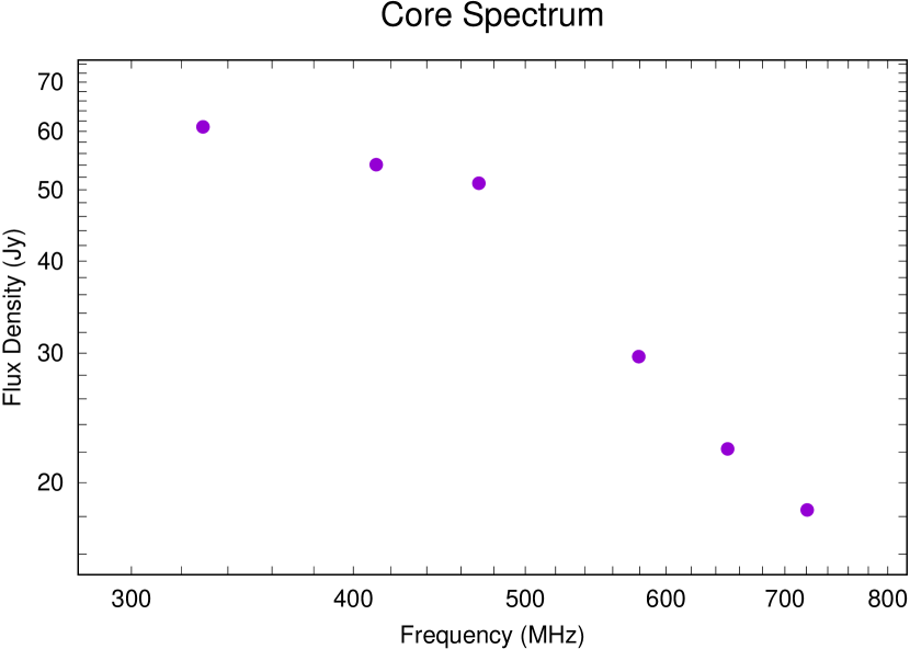
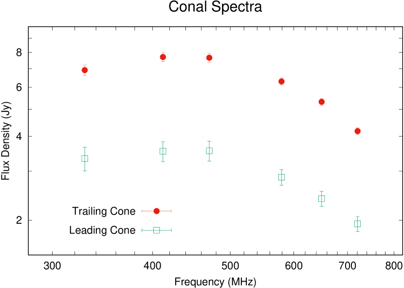
Figure 3: The left plot shows the average Flux density of the core component measured at the 6 frequency bands between 300 MHz and 750 MHz. The right panel shows the corresponding measurements for the leading and trailing conal components. All three components show the transition from the steep spectral behaviour above 470 MHz, to a much flatter spectra below it. The core component has a power law spectral behaviour at the lower frequency range, while the conal components show flat spectra with slight turnover.

The profile of PSR J0332+5434 consists of three main components, a pair of leading and trailing cones as well as a prominent composite central core, that are well separated from each other. We have estimated the average flux densities of all three components at the 6 subbands. The component windows used for the flux estimation were selected to be between 10% level of the peak intensities. Fig 3 shows the spectral nature of the three components between 300 MHz and 750 MHz, with all three components shifting from a steep power law spectra to a much flatter behaviour around 470 MHz. The core component maintains a negative power law spectrum below 470 MHz, but the conal components show slight turnover in their spectral shape with a positive spectral index.

The high intensity level of the pulsar in certain instances saturated the telescope response, where the peak intensities of the core component in the single pulses exceeded the detection limit and were suppressed. One clear indication of saturation was that the linear polarization level (L = $\sqrt{\rm{Q}^{2}+\rm{U}^{2}}$) in these time samples was much higher than the total intensity. We carefully examined the entire pulse sequence and found saturation affecting less then 10% of the single pulses in each subband and limited to less than 5% of the emission window. It is unlikely that the flux estimates from the images are affected by the saturation effect as they were recorded for longer integration time, such that the averaged peak intensity levels were significantly lower. In order to mitigate the effect of saturation on the subsequent analysis, firstly additional contribution from saturation are included in the error estimation of the flux scaling, that may arise from the underestimation of the average intensity of the profile. Secondly, in the spectral analysis of the time samples reported in the subsequent sections we consider only the conal regions that have much lower intensity levels and are free from saturation effect.

2.2 Measuring Polarized Single Pulse Emission

The Band-3 and Band-4 receiver systems of GMRT are equipped with dual linear polarization feeds that are converted into left and right hand circular polarization signals using a quadrature hybrid. The emission from PSR J0953+0755 was also recorded during these observations and served as a polarization calibrator. The auto and cross polarized signals of each time sample were suitably calibrated to produce the four Stokes parameters (I, Q, U, V) for each frequency channel (see Mitra et al., 2016, for details). Finally, using the dispersion measure, DM = 26.7641 pc cm^-3, and rotation measure, RM = -64.33 rad m^-2, of PSR J0332+5434 the systematic changes in the polarization behaviour across frequencies were corrected and subsequently averaged to produce the single pulse polarimetric time series corresponding to the 6 subbands. The effect of cross-coupling in the antenna feeds have not been addressed during this analysis and can lead to systematic errors up to 10% of the measured Stokes parameters. The four Stokes parameters of the single pulses in each subband were flux calibrated using the scaling factors from interferometric measurements (see discussion in the previous subsection). The two GMRT subarrays recorded independently and thereby introduced an arbitrary phase shift between the PPA traverse of Band-3 and Band-4 measurements that was estimated by careful visual inspection. The two Stokes parameters Q and U of one of the bands were rotated appropriately with this phase shift to align the PPA distribution across the entire frequency range. An overlay of the average stokes parameters for all the subbands after correcting for the above effects is shown in the right panel of Fig 2.

3 High Linearly Polarized Time Samples and their Spectral Nature

Figure 4: The above plots show the polarization behaviour of PSR J0332+5434 averaged over the entire 400 MHz frequency range, between 300 MHz and 750 MHz. The left panel comprises of all observed time samples, the middle panel corresponds to the high linearly polarized time samples with L/I $\geq$ 0.85, while the right panel includes the time samples with L/I below 50%. The upper window in each panel shows the average profiles formed from the different time samples consisting of I (black), L (red) and V (blue). The bottom window shows the distribution of the PPAs of the time samples in colour scale along with the RVM fits (magenta) for this pulsar obtained from the PPA distribution shown in Fig 5 (see discussion in section 3).

Figure 5: The figure shows the polarization behaviour of PSR J0332+5434 averaged over 400 MHz bandwidth between 300 MHz and 750 MHz. The figure uses time samples with L/I above 85% in single pulses with weaker emission in the core region, i.e. less than one tenth of the maximum detection sensitivity. The left panel is similar to Fig. 4 (see caption therein for details), while the right panel shows the number of time samples in each longitude bin used for the left plot, with clear demarcation for the longitude ranges corresponding to the leading cone, core and trailing cone shown in the figure.

Fig. 4, left panel, shows the polarization behaviour of PSR J0332+5434 averaged for 400 MHz within the 300 MHz and 750 MHz frequency range. The peaks of the 6 subbands were aligned before averaging (see Fig. 2, right panel) and included time samples with significant polarization detection, i.e. linear polarization level above five times the baseline noise rms of each single pulse. The two parallel RVM like PPA tracks can be readily seen in the lower window, although some PPA samples also spread out between the tracks and there is significant deviation from RVM in the core region, which has also been noted in Edwards & Stappers (2004). Mitra et al. (2023a) showed that the PPA traverse of highly polarized time samples can uncover the underlying RVM nature in pulsars with complicated PPA distribution. The middle panel of Fig. 4 picks out the high linearly polarized time samples, L/I exceeding 85%, where the PPAs are mostly along the two orthogonal RVM tracks. The right panel of Fig. 4 comprises of the low polarization signals, L/I below 50%, with the orthogonal RVM nature in the PPA distribution is discernible amidst the non-orthogonal behaviour. Initial results identifying the high linearly polarized emission from these observations over a limited frequency range, between 550 MHz and 750 MHz, have been previously reported in Mitra et al. (2024). These results are consistent with the general trend seen in the normal pulsar population (Johnston et al., 2024).

Although, the spread in the PPA distribution reduces in the high linearly polarized profile (middle panel, Fig. 4), there still remains considerable deviation from the RVM nature below the core window within -6^∘and $5^{\circ}$. Mitra et al. (2007) showed that the distortion of the PPA distribution in core region disappears in the single pulses where the core intensity is weaker. The high linearly polarized average profile is reconstructed by considering the single pulses with lower intensity core emission, i.e. less than 10% of the maximum detection sensitivity recorded in the core region of the single pulses, and shown in Fig. 5, left panel. Note that although our selection criteria was set to choose weak flux points in the core region, still about 10 time samples with high flux got selected. This is due to the fact that the noise level in some single pulses were extrememly high and hence the the signal to noise for these high flux samples were low and fitted the selection criteria. We have retained these points since they do not affect the PPA distribution. The overall distortion in the PPA distribution is significantly reduced in the core region and they follow two parallel tracks. This updated distribution is used to estimate the RVM fits for PSR J0332+5434 at the observing frequency using the equation,

$$\Psi=\Psi_{\circ}+\tan^{-1}{\left(\frac{\sin{\alpha}\sin{(\phi-\phi_{\circ})}}{\sin{(\alpha+\beta)}\cos{\alpha}-\sin{\alpha}\cos{(\alpha+\beta)}\cos{(\phi-\phi_{\circ})}}\right)}.$$ (1)

Here $\Psi$ is the PPA from RVM, $\phi$ is the rotational phase, $\alpha$ is the angle between the rotation and magnetic axes, and $\beta$ is the angle between the rotation axis and the observer’s line of sight during their closest approach. $\Psi_{\circ}$ and $\phi_{\circ}$ defines the reference points for measurement offsets in $\Psi$ and $\phi$, respectively. We have used eq.(1) to find appropriate fits of the emission geometry from the measured PPA using $\chi^{2}$ minimization techniques and obtain the minimum reduced $\chi^{2}\sim 6.5$ with corresponding values of the parameters as $\alpha=46.8^{\circ}$, $\beta=-4.5^{\circ}$ and $\phi_{\circ}=0.8^{\circ}\pm 0.4^{\circ}$. However, it has been well established that the geometric angles $\alpha$ and $\beta$ obtained from RVM fitting are highly correlated and should be treated with caution (see e.g. Everett & Weisberg 2001). The orthogonal RVM fits to the PPA distribution are shown in as Fig 4 as well as the left panel of Fig. 5 (magenta curves). The solid magenta curve specifies the primary polarization mode (PPM) corresponding to $\psi_{\circ}=44^{\circ}\pm 5^{\circ}$, while the orthogonal dashed curve represents the secondary polarization mode (SPM) with $\psi_{\circ}=-46^{\circ}\pm 5^{\circ}$. The right panel in Fig. 5 presents the number of time samples in each longitude range where L/I exceeds 85%, with the added constraint of single pulses having lower intensity core emission.

3.1 Selecting Single Pulse Emission Features for Spectral Studies

In the observing frequency range, between 300 MHz and 750 MHz, the single pulse emission have similar shapes indicating a broadband nature, which is consistent with the results of K03. There are several examples of high linearly polarized signals in the single pulses seen across all 6 subbands. But there is large variability in single pulse structure often in the form of sporadic illumination at different regions of the emission window. Both wider features spanning several degrees of longitude and narrow spiky emission about a degree in width is seen in different pulses. The spiky features are often highly polarized and appears at the same longitude range at all frequencies, and due to their relative ease of identification we particularly focus on their spectral nature in the subsequent analysis.

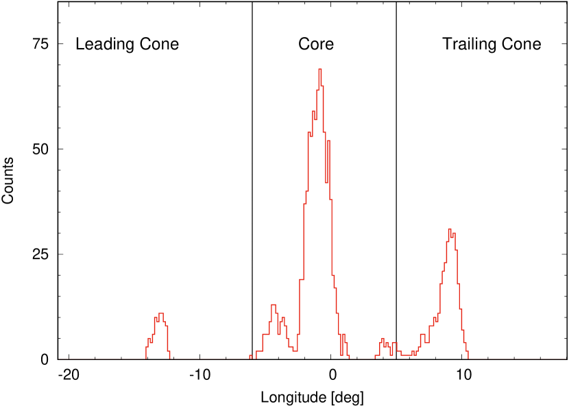
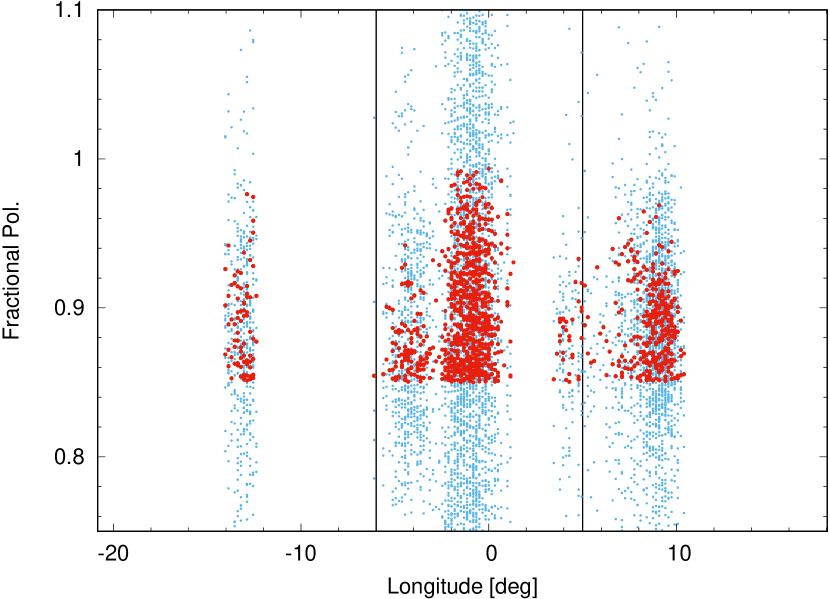
Figure 6: The selection criteria for the band averaged time samples with high levels of linear polarization are, L/I exceeds 85% and they have significant detection sensitivity, exceeding 15 times the noise rms levels in the single pulse baselines. The left panel in the figure shows the number of points in each longitude range that satisfy the selection criteria. The right panel shows the linear polarization fractions of these time samples across the profile window, with the red points representing the average over the entire frequency range, while the blue points correspond to the 6 subbands showing a larger spread than the average. The longitude windows of the leading cone, core and trailing cone are also shown in the figure.

The high linearly polarized time samples in the single pulses have been identified in Fig 4, middle panel, from the 400 MHz band between 300 to 750 MHz, and constitute L/I $\geq$ 85% and significant linear polarization detection sensitivity above 5 times the noise rms levels of the single pulse baselines. However, in the individual subbands the linear polarization levels of these time samples show a larger spread, often due to higher noise levels in each subband and consequently lower detection sensitivity. In order to minimise the spread the selection criterion is tightened to include time samples with detection sensitivity above 15 times the baseline noise levels and at least five times above the noise levels for each individual subband. Fig. 6, left panel, shows the number of time samples at each longitude bin that satisfy this section criterion. We have limited the spectral studies to the conal region of the pulsar profile, excluding the core between longitude range of -6$\arcdeg$ and 5$\arcdeg$ (see discussion in the previous section about saturation in the core). In some instances the L/I exceeds 100% which is unphysical, but in realistic measurements this can be attributed to cumulative errors like statistical fluctuation in the linear polarization, improper removal of polarization baseline levels, high baseline noise, cross-coupling between different polarizations, etc. Attributing an additional 10% error due to these effects the spectral studies are restricted to time samples in 6 subbands with L/I between 75% and 110%. Fig. 6, right panel, shows the distribution of the L/I for the selected time samples across the profile window.

The above selection criteria yielded a total of 93 high linearly polarized time samples, with about 34% samples belonging to the leading cone and 66% to the trailing conal component. The widths of the emission features associated with the high linearly polarized time samples, obtained from the full band, have been estimated at 50% level (W₅₀) of their peak intensity, and the distribution of the widths corresponding to the leading and trailing cones is shown in Fig. 7. More than 70% of these are narrow spiky features with widths less than 1.5$\arcdeg$ in longitude (see examples in Fig. 8), compared to around 3$\arcdeg$ for the leading and trailing conal components in the average profile. In the leading conal side around 90% of the highly polarized features belong to the narrow spiky category, while there is more even distribution in the trailing cone, with around 60% narrow features and the remaining 40% wider features with widths in excess of 1.5$\arcdeg$. The spiky emission is localised within a narrow longitude range across all 6 subbands with their peaks being mostly coincident.

The narrow localized nature of the spiky emission bears resemblance to the quasi-periodic emission structures found in single pulses of certain pulsars, known as microstructures (Boriakoff, 1983; Popov et al., 1987; Smirnova et al., 1994). Several studies have found strong correlation between microstructure widths ($w_{\mu}$) and the pulsar period with a dependence, $w_{\mu}\approx 0.5\times 10^{-3}P$ (Taylor et al., 1975; Cordes, 1979; Kramer et al., 2002; Mitra et al., 2015). Using this relation the expected microstructure width in PSR J0332+5434, with $P=0.714$ seconds, is $w_{\mu}\sim 357$ $\mu$s. This is comparable to the observing time resolution, 327 $\mu$s, and hence microstructures cannot be detected from these measurements. Additionally, the spiky highly linearly polarized emission is much wider than the expected microstructures and appear to be unrelated to them.

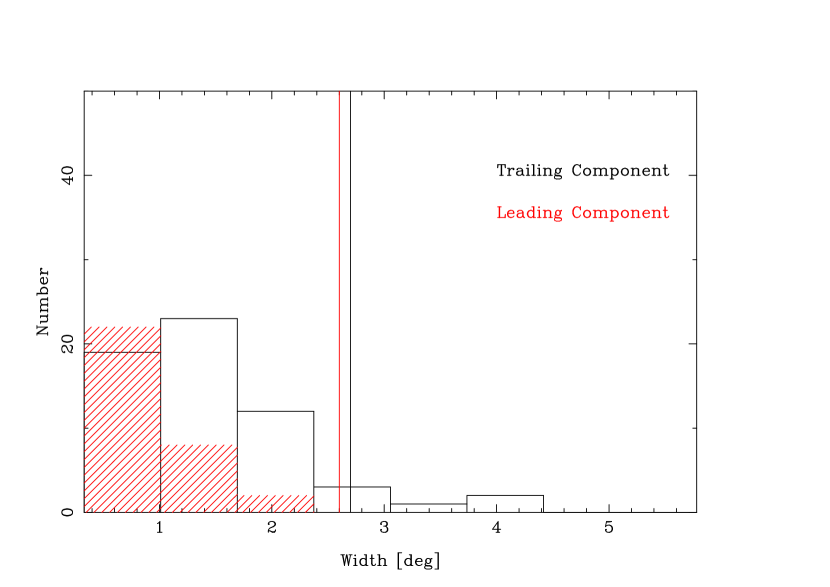
Figure 7: The figure shows the distribution of the widths of the highly polarized emission features in PSR J0332+5434 measured over 400 MHz band, between 300 MHz and 750 MHz, and obtained using our selection criteria (see text for details). The red distribution corresponds to features seen in the leading conal window while the black histogram represents the features in the trailing conal side. The widths were estimated at 50% level of the peak intensity. The corresponding widths for the leading and trailing cone in the average profile is shown as vertical red and black lines, respectively.

3.2 Spectral Nature of Highly Polarized Emission

Figure 8: The figure shows four single pulses of PSR J0332+5434 containing high linearly polarized spiky emission, exemplifying their polarization behaviour as well as spectral nature. Each panel comprises of three separate windows, where the left window shows the single pulse I, L and V at the 6 subbands between 300 MHz and 750 MHz as well as the average behaviour across the entire band at the bottom. The dashed lines in the figures identify the spiky emission from the full band, specified by $W_{50}$ of the feature. The top window on the right shows the PPA distribution across the single pulse for all 6 frequencies (see caption in Fig.2 for the frequency colour code). The PPAs of the spiky emission belong to the PPM in all cases. The bottom window on the right shows the spectral nature of the spiky polarized emission, where the average intensities at the 6 frequencies are estimated within the dashed window. (a) Pulse number 1051 where the spiky emission is seen in the trailing cone and the spectrum turns over with peak around 600 MHz. (b) Pulse number 2496 with the spiky emission in the leading cone and the spectrum reverses to positive spectral index around 600 MHz. (c) Pulse number 5220 with the spiky emission in the leading cone and the spectrum flattens at lower frequencies below 400 MHz. (d) Pulse number 6004 where the leading cone contains the spiky emission that has a inverted parabolic spectrum peaked around 500 MHz.

Figure 9: The figure shows an expanded view of the highly polarized spiky features in the four pulses reported in Fig. 8, at frequencies 330 MHz (red), 412 MHz (green), 470 MHz (blue), 580 MHz (orange), 638 MHz (yellow) and 720 MHz (indigo). The dot-dashed lines in the background of each panel show the relevant conal components of the average profiles at these frequencies, trailing cone in the left panels and leading cone in the right panels, with the same frequency colour scheme, and intensities scaled appropriately to be visible within the window. The average profile as well as the single pulses in each frequency have been aligned such that the profile peak is at zero longitude. The effect of RFM is readily seen in the cones, i.e. the emission shifts outward from the center with decreasing frequency. But this phenomenon is absent in the spiky emission, where the emission windows at different frequencies show little shift usually within one or two longitude bins.

The spectra of highly polarized emission features are estimated using $W_{50}$ window from the full band to find the average flux density at each frequency. Fig. 8 shows the emission behaviour of the spiky highly polarized features in four single pulses, pulse numbers 1051, 2496, 5220 and 6004 from the start of the observing session. The left window in all four panels, show the intensity in the single pulses corresponding to I, L and V at all 6 subbands as well as the full 400 MHz band, where the $W_{50}$ window has been identified with dashed lines. The spiky emission is seen within the trailing cone in pulses 1051 and 5220, but in the leading conal side in pulse 2496 and 6004. The top window on the right side shows the PPA distribution at all 6 frequencies while the bottom window represents the estimated spectrum obtained from the average flux estimates.

The spiky features in all cases have a broadband character and appear almost in the same longitude range at all frequencies. This is highlighted in Fig. 9 showing the expanded view of spiky emission features across the frequency range, overlaid on the relevant average conal component at these frequencies. The features are narrower than the cones and are largely localised within a narrow longitude range. In contrast both the leading and trailing conal components clearly show the effect of radius to frequency mapping (RFM), according to which the profile width progressively increases with decreasing frequency. The average emission at different frequencies are expected to originate from different heights in the pulsar magnetosphere, with higher frequencies arising closer to the stellar surface. However, the lack of RFM in the spiky emission suggests that they are localised within the magnetosphere, with the same source emitting over the frequency range of detection.

The spectra of these features have a variety of shapes, the most noticeable being the inverted spectra with a turnover frequency (see spectra of pulses 1051 and 6004 in Fig. 8) and the spectra falling on either side of the turnover frequency resembling a inverted parabolic shape and further the spectra differs greatly from the average spectra of the cones (see right panel of Fig. 3). The turnover frequencies in these inverted parabolic spectra are not fixed but shift within the entire band, e.g. the turnover frequency is around 600 MHz in pulse number 1051 but shifts to 500 MHz in pulse 6004. We found 42 spiky features with inverted parabolic spectral shape, constituting around 60% of the total sample. The spectra show flattening at the lower frequencies in several cases, while at other instances the spiky feature merge with surrounding emission and the resultant spectra in the $W_{50}$ window has irregular shape. The PPAs in all spiky features follow the RVM and are associated exclusively with the PPM.

Figure 10: The above plot shows two examples of single pulses from PSR J0332+5434 containing high linearly polarized broad emission features. The details of the individual panels are identical to Fig. 10 (see caption there for description). However, unlike the spiky emission the PPAs of the wide features are seen along both the PPM and the SPM. (a) Pulse number 3109 where the broad highly polarized emission is seen in the leading cone and the spectrum is mostly inverted power law with flattening above 600 MHz. (b) Pulse number 3356 where the broad emission is seen in the trailing cone and the spectrum has irregular shape.

Figure 11: The figure shows an expanded view of the highly polarized broad features in the two pulses reported in Fig. 10. The figure is identical to Fig. 9 (see caption for description). The broad features mostly match the radius to frequency mapping of the conal components.

In addition to the spiky features there are several examples of broader features with W${}_{50}>1.5\arcdeg$, that exhibit high levels of L/I. Examples of these features are seen in pulse number 3109 at the location of the leading cone and in trailing conal side of pulse number 3356, as shown in Fig. 10. The wider features are clearly different from the spiky emission in their physical properties. There are a few examples of inverted parabolic spectral shape even in these wider features, but they constitute less than 20% of the total sample. In most instances the spectra have irregular shape, but the flux generally decreases with increasing frequency. A closer look into the wider features shown in Fig. 11 reveal that they largely follow the tendency of RFM, consistent with the average conal behaviour. Although the PPAs in these features follow the RVM, they can be associated with both the PPM and the SPM.

4 Spectral nature of high linearly polarized emission : Qualitative Concepts

The polarization behaviour is expected to be a direct consequence of the underlying radio emission mechanism in pulsars. But the observed spectra is likely to be different from the one obtained from the intrinsic emission mechanism as they get reshaped through a number of subsequent processes, like averaging of emission from multiple sources with shifted spectra, propagation in the pulsar magnetosphere as well as the intervening medium, the observers’ line of sight geometry, etc. In the remainder of this section we will carry out a qualitative discussion about the origin of polarization from the emission mechanism as well as the effect of different phenomena on the observed spectra from pulsars, starting from the role of the emission mechanism. A more detailed quantitative study to model the observed average spectra as well as from the different single pulse polarized features will be deferred to a future dedicated work (see Basu et al., 2022b, for details).

The first and most important step towards understanding the radio emission mechanism is determining the location of the emission region in the pulsar magnetosphere. A widely used technique for estimating the radio emission height utilizes the aberration and retardation (A/R) effect arising due to rotation of the pulsar, which causes a shift ($\Delta\phi$) of the profile window with respect to the magnetic axis. The emission height, $h$, is related to this shift as $\Delta\phi=1440h/Pc$, where $\Delta\phi$ is in degrees, $c$ is the velocity of light and $P$ is the pulsar period (Blaskiewicz et al., 1991). The longitude difference between the profile center and the SG point ($\phi_{\circ}$) of the PPA traverse gives measure of $\Delta\phi$ from observations. As shown earlier, the PPAs of PSR J0332+5434 can be used to obtain RVM fits with estimates of $\phi_{\circ}=0.8\arcdeg\pm 0.4\arcdeg$. The outer edges of the average profile from the full band, estimated at 10% level of the conal components, are located at $\phi_{l}=-16.3\arcdeg\pm 0.4$ in the leading side and $\phi_{t}=12.7\arcdeg\pm 0.4$ in the trailing side. The profile center is located at -1.8$\arcdeg$ and using $P=0.715$ seconds, gives estimate of the average profile height to be $h\sim 386\pm 85$ km, which is well below 10% of the light cylinder radius ($Pc/2\pi\sim 35000$ km). The PPM and SPM fit orthogonal RVM models with identical $\phi_{\circ}$, suggesting similar emission heights for both modes.

The pulsar magnetosphere is filled with a dense electron-positron pair plasma streaming outwards in a relativistic non-stationary flow along the open field lines. The estimated emission height suggests the coherent radio emission to be excited in the strongly magnetized limit, and if we consider identical distribution functions of electrons and positrons, then the dispersion equations describing this system yield two orthogonal linearly polarized modes, the ordinary (O-mode) and extraordinary (X-mode) mode. The polarization vector of O-mode lies in the plane of propagation vector, $\vec{k}$, and the ambient magnetic field, $\vec{B}$, with a component along $\vec{B}$ as well as $\vec{k}$. The X-mode, has transverse character where the polarization vector is directed perpendicular to the plane containing $\vec{k}$ and $\vec{B}$, and is also known as $t$-mode. There are two additional branches of the O-mode, $lt_{1}$-mode and $lt_{2}$-mode, that are mixed longitudinal-transverse in nature. The $lt_{1}$-mode is sub-luminal and when propagating along the magnetic field it is an arbitrarily polarized purely transverse wave, while during oblique propagation it has longitudinal-transverse character. The $lt_{2}$-mode during oblique propagation has longitudinal-transverse nature and is super-luminal for low wave numbers but can transform into sub-luminal waves at high frequencies. When propagating along the magnetic fields the $lt_{2}$-mode coincides with the electrostatic Langmuir mode.

There is growing evidence that the PPAs of high linearly polarized time samples in pulsars follow the RVM, similar to PSR J0332+5434, with two orthogonal tracks. CCR is the only known mechanism that can excite waves polarized parallel and perpendicular to the curved magnetic field line planes such that the polarization vector of the emission can exhibit orthogonal RVM characteristics (Mitra et al., 2009, 2023a, 2023b). As a result the observed PPM and the SPM of the highly polarized signals can be readily associated with the X (or $t$-mode) and O (or $lt$-mode) modes in the strongly magnetized pair plasma, polarized either perpendicular or parallel to the curved magnetic field line planes, respectively. The association of the PPA with the X-mode has been established in the radio emission from the Vela pulsar. The X-ray observations was used to determine its projected rotation axis in the sky plane while the SG point of the PPA traverse provided the location of the dipolar magnetic fiducial plane. The difference between the projected angle of the rotation axis and the PPA at the SG point is $\sim 90\arcdeg$, suggesting that the emerging polarization is perpendicular to the dipolar magnetic fiducial plane, i.e. like the X-mode (Helfand et al., 2001). Only one PPA track is observed in the Vela pulsar such that the O-mode is absent. Unfortunately, it has not been possible to determine the direction of the rotation axis in other pulsars, hindering direct measurement of the orientation of the emerging radiation. However, the proper motion (PM) of Vela pulsar is along its rotation axis, and if this is a general trend in pulsars then the difference between the PM and the PPA at the SG point can be used as a substitute to find the direction of the emerging radiation. In PSR J0332+5434, Mitra et al. (2007) estimated $\mid$PM-PPA$\mid$ for the PPM to be $\sim 100\arcdeg$, which is nearly orthogonal to the magnetic fiducial plane, and suggested the PPM to be associated with the X-mode, and as a corollary the SPM can be identified as the O-mode. However, such associations need to be treated with caution, since the orientation of PM to be along the rotation axis is not an established fact in the general pulsar population. PSR J0332+5434 is a relatively old pulsar and the Galactic potential may have changed the direction its PM away from the natal kick along the rotation axis (Noutsos et al. 2013). However, if we ascribe the PPM to the X-mode then the spiky emission is a feature of the X-mode. The broad highly polarized features exhibit PPM as well as SPM and hence can associated with both the X-mode and O-mode.

The high linearly polarized spiky emission are correlated across the entire frequency range and do not show any signature of RFM. This suggests that the CCR leading to these spiky features must arise from a narrow range of emission heights. A suitable candidate for charge bunches giving rise to CCR is the stable relativistic charged envelopes or solitons that can form in the pulsar plasma (Melikidze et al. 2000; Lakoba et al. 2018; Rahaman et al. 2022). The two stream instability develops in the non-stationary plasma and facilitates the linear growth of Langmuir waves. The modulational instability of the Langmuir waves leads to the formation of charged solitons. The charged solitons move along curved magnetic field lines and emit curvature radiation to excite the $t$ and $lt_{1}$ modes. In the presence of strong magnetic field the refractive indices in the plasma are different for $t$ and $lt_{1}$ modes, resulting in different phase velocities. The $t$-mode (X-mode) has vacuum like character and can escape readily from the plasma. The $lt_{1}$ mode (O-mode) gets ducted along the magnetic field lines, and can only escape from the plasma boundary. The non-stationary plasma flow is generated from sparking discharges in an inner acceleration region (IAR) above the polar cap, which is partially screened by ions emitted from the stellar surface (see Basu et al., 2022a, for description of the sparking process). The sparking process forms dense intermittent plasma clouds outside the IAR that flows outward along the magnetic field lines, interspersed with less dense regions. At the radio emission region a large number of solitons are formed in these dense plasma clouds. The radio emission detected by the observer is obtained from incoherent addition of a large number of solitons, each emitting CCR.

The curvature radiation spectrum from a single soliton in vacuum, of size $a_{s}$ and Lorentz factor $\gamma_{s}$, moving along strong magnetic field, with radius of curvature $\rho$, has been estimated by Melikidze et al. (2000). The soliton in plasma moves with the group velocity with Lorentz factor being slightly larger than the plasma. When compared with the single particle spectra the soliton spectra has an extra term $[1-\cos(a(\omega/\omega_{c})]^{2}$, where $a=a_{s}{\gamma_{s}}^{3}/\rho$ and the characteristic frequency $\omega_{c}=1.5{\gamma_{s}}^{3}(c/\rho)$. These differences causes the curvature radiation spectra of solitons to have characteristic frequency to be a few times greater than the single particle $\omega_{c}$ and the spectra is wider and more symmetrical (see Fig 4. of Melikidze et al. 2000). The soliton spectra power falls off on either side of the characteristic frequency and has an upper cutoff frequency, $\nu_{h}\sim c/a_{s}$, below which the emission remains coherent. In the presence of plasma the emission from soliton is modified in a few different ways. Firstly, the emission splits into the $t$ and $lt$ modes such that the power in the $t$ mode is seven times weaker than the $lt$ mode. This reduction of power is uniform across all frequencies, ensuring that the spectral shape remains unchanged. Secondly, the emission can get suppressed within the plasma. Gil et al. (2004) showed that the $t$-mode is largely suppressed compared to the vacuum case, however can still escape freely preserving its inherent vacuum like polarization properties and spectral shape and can also explain the observed pulsar luminosities. The $lt$ mode can get entirely damped, and requires special regions such as the plasma edge at the boundary between clouds to escape (Melikidze et al. 2014; Mitra et al. 2023b). Next, if the distance between the solitons in the plasma is $D_{s}$, there is a lower frequency cutoff in the spectrum $\sim c/D_{s}$. Finally, the resultant spectrum is formed after incoherent addition of emission from a large number of solitons and can deviate from a single soliton spectral shape due to variations in several parameters such as $a_{s}$, $\gamma_{s}$, $\rho$, $D_{s}$, etc (see Basu et al. 2022b).

The absence of RFM in the spiky polarized features (see Fig. 9) can be interpreted as the emission arising from a single plasma cloud due to incoherent addition of CCR from a large number of solitons. In many of these features the spectra have inverted parabolic shapes, e.g. the two pulses shown in Fig. 8, pulse number 1051 with $\nu_{c}\sim 600$ MHz and pulse 6004 with $\nu_{c}\sim 500$ MHz. At the emission height of $\sim$ 300 km, we estimate $\rho\sim 3\times 10^{8}$cm in the conal region, which implies $\gamma_{s}\sim$ 300 for these characteristic frequencies. This shows that spectral shapes with different characteristic frequencies can be obtained from small variations in $\gamma_{s}$. However, estimating the other parameters like $a_{s}$ and $D_{s}$ requires measurements over a wider frequency range. The broader polarized features (see Fig. 10 and 11) on the contrary show RFM, indicating that the different frequencies arise from a range of heights. In this case several clouds from different heights contribute to the emission at any given frequency in a manner consistent with RFM in the average feature. The resultant spectrum is composed of emission from different clouds, where each cloud is characterized by different estimates of the parameters $a_{s}$, $\gamma_{s}$ and $D_{s}$. Thus the observed spectra reflects an average of the distribution of the parameters, and cannot uniquely represent a single soliton spectrum. A proper modeling of the spectra requires detailed simulations which is beyond the scope of this work, and will be addressed in future studies.

5 Summary

In this work we have used observations of PSR J0332+5434 over a wide frequency range, between 300 MHz and 750 MHz, to study the behaviour of high linearly polarized emission features in the single pulses as a function of frequency. The time samples with high levels of linear polarization across the entire frequency range have their PPAs distributed along two parallel tracks that follow the RVM. The two tracks, divided into PPM and SPM, can be associated with X-mode and O-mode in a strongly magnetized plasma. Using predictions of the A/R effect, the location of the radio emission region in PSR J0332+5434 at the observing frequencies is found to be few hundred km above the neutron star surface. At the location of radio emission, the polarization behaviour strongly favours the CCR from charged bunches as the radio emission mechanism. In the strongly magnetized, relativistic pair plasma in the pulsar magnetosphere, with a non-stationary flow along the open field lines, charged solitons are expected to form, and are the likely candidates for the charged bunches producing CCR.

We find several examples of high linearly polarized narrow spiky emission features whose location within the profile is roughly constant across the frequency range. This emission is always associated with the PPM, and can also possibly be associated with the X-mode. We suggest that this spiky emission arises from a single plasma cloud with incoherent addition from a large number of solitons, each emitting CCR. We detected many cases where the spectra of the spiky emission features have inverted parabolic shapes, that resemble the soliton spectrum. This further implies that in an emission cloud there is little spread in the values of soliton size, $a_{s}$, inter soliton distance, $D_{s}$ and Lorentz factor of the solitons, $\gamma_{s}$. The peak of the inverted spectrum can be used to find $\gamma_{s}$ which is of the order of a few hundred. There are also examples of high linearly polarized emission features with much broader size. These features seem to follow the RFM seen in the average profile, and it can be interpreted that their emission arise from a range of heights. The spectra of these features are formed after averaging over many clouds that have different distribution of soliton parameters. This provides a qualitative description of the origin of RFM in pulsars, although more detailed quantitative estimates are necessary to understand how the averaging process works in practice.

References

- Basu et al. (2022a) Basu, R., Melikidze, G. I., & Mitra, D. 2022a, ApJ, 936, 35, doi: 10.3847/1538-4357/ac8479
- Basu et al. (2021) Basu, R., Mitra, D., & Melikidze, G. I. 2021, ApJ, 917, 48, doi: 10.3847/1538-4357/ac0828
- Basu et al. (2022b) —. 2022b, ApJ, 927, 208, doi: 10.3847/1538-4357/ac5039
- Blaskiewicz et al. (1991) Blaskiewicz, M., Cordes, J. M., & Wasserman, I. 1991, ApJ, 370, 643, doi: 10.1086/169850
- Boriakoff (1983) Boriakoff, V. 1983, ApJ, 272, 687, doi: 10.1086/161331
- Cole & Pilkington (1968) Cole, T. W., & Pilkington, J. D. H. 1968, Nature, 219, 574, doi: 10.1038/219574a0
- Cordes (1979) Cordes, J. M. 1979, Australian Journal of Physics, 32, 9, doi: 10.1071/PH790009
- Cordes & Rickett (1998) Cordes, J. M., & Rickett, B. J. 1998, ApJ, 507, 846, doi: 10.1086/306358
- Edwards & Stappers (2004) Edwards, R. T., & Stappers, B. W. 2004, A&A, 421, 681, doi: 10.1051/0004-6361:20040228
- Everett & Weisberg (2001) Everett, J. E., & Weisberg, J. M. 2001, ApJ, 553, 341, doi: 10.1086/320652
- Gangadhara & Gupta (2001) Gangadhara, R. T., & Gupta, Y. 2001, ApJ, 555, 31, doi: 10.1086/321439
- Gil et al. (2004) Gil, J., Lyubarsky, Y., & Melikidze, G. I. 2004, ApJ, 600, 872, doi: 10.1086/379972
- Gil & Lyne (1995) Gil, J. A., & Lyne, A. G. 1995, MNRAS, 276, L55, doi: 10.1093/mnras/276.1.L55
- Gupta et al. (2017) Gupta, Y., Ajithkumar, B., Kale, H. S., et al. 2017, Current Science, 113, 707, doi: 10.18520/cs/v113/i04/707-714
- Helfand et al. (2001) Helfand, D. J., Gotthelf, E. V., & Halpern, J. P. 2001, ApJ, 556, 380, doi: 10.1086/321533
- Jankowski et al. (2018) Jankowski, F., van Straten, W., Keane, E. F., et al. 2018, MNRAS, 473, 4436, doi: 10.1093/mnras/stx2476
- Johnston et al. (2024) Johnston, S., Mitra, D., Keith, M. J., Oswald, L. S., & Karastergiou, A. 2024, MNRAS, 530, 4839, doi: 10.1093/mnras/stae1175
- Kramer et al. (2002) Kramer, M., Johnston, S., & van Straten, W. 2002, MNRAS, 334, 523, doi: 10.1046/j.1365-8711.2002.05478.x
- Kramer et al. (2003) Kramer, M., Karastergiou, A., Gupta, Y., et al. 2003, A&A, 407, 655, doi: 10.1051/0004-6361:20030842
- Lakoba et al. (2018) Lakoba, T., Mitra, D., & Melikidze, G. 2018, MNRAS, 480, 4526, doi: 10.1093/mnras/sty2152
- Maron et al. (2000) Maron, O., Kijak, J., Kramer, M., & Wielebinski, R. 2000, A&AS, 147, 195, doi: 10.1051/aas:2000298
- Melikidze et al. (2000) Melikidze, G. I., Gil, J. A., & Pataraya, A. D. 2000, ApJ, 544, 1081, doi: 10.1086/317220
- Melikidze et al. (2014) Melikidze, G. I., Mitra, D., & Gil, J. 2014, ApJ, 794, 105, doi: 10.1088/0004-637X/794/2/105
- Mitra (2017) Mitra, D. 2017, Journal of Astrophysics and Astronomy, 38, 52, doi: 10.1007/s12036-017-9457-6
- Mitra et al. (2015) Mitra, D., Arjunwadkar, M., & Rankin, J. M. 2015, ApJ, 806, 236, doi: 10.1088/0004-637X/806/2/236
- Mitra et al. (2016) Mitra, D., Basu, R., Maciesiak, K., et al. 2016, ApJ, 833, 28, doi: 10.3847/1538-4357/833/1/28
- Mitra et al. (2024) Mitra, D., Basu, R., & Melikizde, G. I. 2024, Universe, 10, 248, doi: 10.3390/universe10060248
- Mitra et al. (2009) Mitra, D., Gil, J., & Melikidze, G. I. 2009, ApJ, 696, L141, doi: 10.1088/0004-637X/696/2/L141
- Mitra et al. (2023a) Mitra, D., Melikidze, G. I., & Basu, R. 2023a, MNRAS, 521, L34, doi: 10.1093/mnrasl/slad022
- Mitra et al. (2023b) —. 2023b, ApJ, 952, 151, doi: 10.3847/1538-4357/acdc28
- Mitra & Rankin (2002) Mitra, D., & Rankin, J. M. 2002, ApJ, 577, 322, doi: 10.1086/342136
- Mitra et al. (2007) Mitra, D., Rankin, J. M., & Gupta, Y. 2007, MNRAS, 379, 932, doi: 10.1111/j.1365-2966.2007.11988.x
- Noutsos et al. (2013) Noutsos, A., Schnitzeler, D. H. F. M., Keane, E. F., Kramer, M., & Johnston, S. 2013, MNRAS, 430, 2281, doi: 10.1093/mnras/stt047
- Perley & Butler (2017) Perley, R. A., & Butler, B. J. 2017, ApJS, 230, 7, doi: 10.3847/1538-4365/aa6df9
- Popov et al. (1987) Popov, M. V., Smirnova, T. V., & Soglasnov, V. A. 1987, AZh, 64, 1013
- Radhakrishnan & Cooke (1969) Radhakrishnan, V., & Cooke, D. J. 1969, Astrophys. Lett., 3, 225
- Rahaman et al. (2022) Rahaman, S. M., Mitra, D., Melikidze, G. I., & Lakoba, T. 2022, MNRAS, 516, 3715, doi: 10.1093/mnras/stac2264
- Rankin (1993a) Rankin, J. M. 1993a, ApJ, 405, 285, doi: 10.1086/172361
- Rankin (1993b) —. 1993b, ApJS, 85, 145, doi: 10.1086/191758
- Rickett (1990) Rickett, B. J. 1990, ARA&A, 28, 561, doi: 10.1146/annurev.aa.28.090190.003021
- Shang et al. (2017) Shang, L.-H., Lu, J.-G., Du, Y.-J., et al. 2017, MNRAS, 468, 4389, doi: 10.1093/mnras/stx815
- Shapakidze et al. (2003) Shapakidze, D., Machabeli, G., Melikidze, G., & Khechinashvili, D. 2003, Phys. Rev. E, 67, 026407, doi: 10.1103/PhysRevE.67.026407
- Smirnova et al. (1994) Smirnova, T. V., Tul’bashev, S. A., & Boriakoff, V. 1994, A&A, 286, 807
- Swainston et al. (2022) Swainston, N. A., Lee, C. P., McSweeney, S. J., & Bhat, N. D. R. 2022, PASA, 39, e056, doi: 10.1017/pasa.2022.52
- Swarup et al. (1991) Swarup, G., Ananthakrishnan, S., Kapahi, V. K., et al. 1991, Current Science, 60, 95
- Taylor et al. (1975) Taylor, J. H., Manchester, R. N., & Huguenin, G. R. 1975, ApJ, 195, 513, doi: 10.1086/153351