Continuity up to the boundary for minimizers of the one-phase Bernoulli problem

Abstract.

We prove new boundary regularity results for minimizers to the one-phase Alt-Caffarelli functional (also known as Bernoulli free boundary problem) in the case of continuous and Hölder-continuous boundary data. As an application, we use them to extend recent generic uniqueness and regularity results to families of continuous functions.

1. Introduction

In this work, we study minimizers of the Alt–Caffarelli functional

(1.1) $$\operatorname{\textit{F}_{\Lambda}}(u,D)\coloneq\int_{D}|\nabla u|^{2}dx+\Lambda|\{u>0\}\cap D|,$$

where $D$ is an open domain in $\operatorname{\mathbb{R}}^{d}$, $\Lambda$ a positive real constant and $u\in H^{1}(D)$.

The problem, also known as one-phase or Bernoulli problem, originates in the fundamental works [Caf77, AC81] and has various applications in models of flame propagation [BL82] and jet flows [ACF82]. Recent development include [JS14, ESV20, ESV24, EFY23, FY23]. We also refer to [CS05] and [Vel23] for a detailed mathematical exposition.

Given an open bounded domain $D\subset\operatorname{\mathbb{R}}^{d}$ and a boundary datum $g\in H^{1}(D)$ with $g\geq 0$ in $D$, the Alt–Caffarelli problem is the minimization:

(1.2) $$\min\{\operatorname{\textit{F}_{\Lambda}}(u,D):u\in H^{1}(D)\text{ such that }u-g\in H_{0}^{1}(D)\}.$$

Any minimizer $u$ is nonnegative, and splits the domain into two parts:

$$\Omega_{u}:=\{x\in D:u(x)>0\}\quad\text{ and }\quad\Omega_{0}:=\{x\in D:u(x)=0\}.$$

The interface between the two sets, $\partial\Omega_{u}$, is a priori unknown and is called the free boundary.

Any minimizer $u$ to (1.2) is locally Lipschitz continuous inside $D$ (see e.g. [Vel23, Chapter 3]). The Euler–Lagrange equation, satisfied by (classical) stationary points of (1.1), is given by

$$\left\{\begin{array}[]{rcll}u&\geq&0&\quad\text{in}\quad D,\\ \Delta u&=&0&\quad\text{in}\quad\Omega_{u},\\ |\nabla u|&=&\sqrt{\Lambda}&\quad\text{on}\quad\partial\Omega_{u}\cap D.\end{array}\right.$$

For general stationary solutions, the previous equations need to be understood in the viscosity sense. Throughout the paper, for the sake of simplicity, we will fix $\Lambda=1$.

Reminiscent of the classical Laplace equation with Dirichlet boundary condition, the main goal of this work is to establish basic regularity estimates up to the boundary for solutions to (1.2). To our knowledge, up until now, the community has been proving such estimates on a need-to-use basis (see [ESV24, FY23]). We hope that this short note can be useful to researchers in contexts where such estimates can be applied. In this direction, we present some examples of applications of our results, namely a comparison principle and generic-type results for minimizers.

1.1. Main results

Our main result says that minimizers of the one-phase problem with continuous boundary datum are continuous up to the boundary. The following result applies, for example, to the case of $C^{1}$ domains.

Theorem 1.1.

Let $d\geq 2$ and $D\subset\operatorname{\mathbb{R}}^{d}$ be an open domain such that

• either $D$ is convex,

• or $D$ is a locally $c$-Lipschitz domain, for some $c$ small enough depending only on $d$.

Let $g\in C(\overline{D})\cap H^{1}(D)$ with modulus of continuity $\omega$ and $\|g\|_{H^{1}(D)}\leq M$ for some $M>0$, and let $u$ be a minimizer to (1.2).

Then, $u\in C(\overline{D})$, with a modulus of continuity depending only on $\omega$, $D$, $\Lambda$, and $M$. That is, for any $\varepsilon>0$, there exists $\delta=\delta(\omega,D,\Lambda,M)$ such that

$$|x-y|<\delta\implies|u(x)-u(y)|<\varepsilon\qquad\forall x,y\in\overline{D}.$$

A priori, as for the case of harmonic functions, the modulus of continuity of $u$ does not need to be the same (nor comparable) to the modulus of continuity of $g$.

This is in contrast to the case of more regular boundary data, where for Hölder coefficients we actually obtain Hölder regularity up to the boundary (again, as for harmonic functions):

Proposition 1.2.

Let $d\geq 2$ and $D\subset\operatorname{\mathbb{R}}^{d}$ be an open bounded $C^{1,\alpha}$ domain. Let $g\in C^{\gamma}(\bar{D})\cap H^{1}(D)$ where $\frac{1}{2}<\gamma<1$, and let $u$ be a minimizer to (1.2). Then, $u\in C^{\gamma}(\overline{D})$ and

$$\|u\|_{C^{\gamma}(\overline{D})}\leq C\left(1+\|g\|_{C^{\gamma}(\partial D)}+\|u\|_{L^{\infty}(D)}\right),$$

where $C$ depends only on $d$, $\gamma$, $\Lambda$, $\alpha$ and $D$ (in particular, through its diameter and $C^{1,\alpha}$ norm; see Definition 2.2).

The previous result is a generalization of the case for $\gamma=1$, originally treated in [ESV24, Appendix B].

1.2. Applications to generic regularity

In the second part of the paper, we apply the continuity up to the boundary to show how to extend the results on generic uniqueness of minimizers from [FY23] to the case of merely continuous data.

Namely, we show:

Proposition 1.3.

Let $d\geq 2$, and let $D\subset\operatorname{\mathbb{R}}^{d}$ be a domain as in Theorem 1.1. Let $g_{t}\in C(\overline{D})\cap H^{1}(D)$ for $t\in(0,1)$ with $\sup_{t\in(0,1)}\|g_{t}\|_{H^{1}(D)}<\infty$ be such that, for all $0<s<t<1$,

1. $g_{t}\geq g_{s}\geq 0$ in $D$, and

2. any connected component of $\{g_{s}>0\}\cap\partial D$ contains $x_{0}$ with $g_{t}(x_{0})>g_{s}(x_{0})$.

Then, there exists a countable subset $J\subset(0,1)$ such that for every $t\in(0,1)\backslash J$, there is a unique minimizer of $F_{\Lambda}(\cdot,D)$ with boundary datum given by $g_{t}$.

Lastly, we also show a generic regularity result for the free boundary. By [Wei99], it is already known that up to a certain critical dimension $d^{*}$ ($4\leq d^{*}\leq 6$, see [JS14]) the free boundary of $u$ is always smooth, i.e. its set of singular points, denoted ${\rm Sing}(u)$, is empty (and in general dimension, it has Hausdorff dimension $d-d^{*}-1$). Thanks to [FY23], generically this dimension can be increased by one if one takes minimizers with Lipschitz boundary data. We generalize the result to a wider class of boundary data:

Theorem 1.4.

Let $d\geq 2$, and let $D\subset\operatorname{\mathbb{R}}^{d}$ be a domain as in Theorem 1.1. Let $g_{t}\in C(\overline{D})\cap H^{1}(D)$ with $g_{t}\geq 0$ for $t\in(0,1)$, $\sup_{t\in(0,1)}\|g_{t}\|_{H^{1}(D)}<\infty$, and

$$g_{t}-g_{s}\geq t-s\quad\text{in}\quad D\quad\text{for all}\quad 0<s<t<1.$$

Let $u_{t}$ denote any minimizer of $F_{\Lambda}(\cdot,D)$ with boundary datum $g_{t}$. Then:

• If $d=d^{*}+1$, there exists a countable subset $J\subset(0,1)$ such that

  $${\rm Sing}(u_{t})=\varnothing\qquad\qquad\text{for every }t\in(0,1)\backslash J.$$

• If $d\geq d^{*}+2$,

  $$\textnormal{dim}_{\operatorname{\mathcal{H}}}\,{\rm Sing}(u_{t})\leq d-d^{*}-2\quad\quad\text{for almost every }t\in(0,1),$$

where ${\rm dim}_{\mathcal{H}}$ denotes the Hausdorff dimension of a set.

Remark 1.5.

As an example, the family $\{g+\lambda\}_{\lambda\in(0,1)}$ with $g:\partial D\to\operatorname{\mathbb{R}}$ nonnegative and continuous, satisfies the assumptions of Proposition 1.3 and Theorem1.4.

Remark 1.6.

Contrary to [FY23], where the family ${g_{t}}$ is required to be equi-Lipschitz continuous, any assumption on equicontinuity becomes redundant and only uniform boundedness of the family ${g_{t}}$ and monotonicity are required.

We finally also refer to Lemma 3.1 for a comparison principle between minimizers with continuous boundary data.

1.3. Structure of the paper

We start by proving, in Subsection 2.1 and by means of a barrier and compactness argument, the quantitative continuity up to the boundary, Theorem 1.1. In Subsection 2.2, we then show Proposition 1.2: for Hölder continuous boundary datum, the minimizer is also Hölder continuous (with the same exponent) up to the boundary. For that, we use a modified version of the arguments in [ESV24, Lemma B.1].

Finally, in Section 3, we apply our results by first proving a general comparison lemma for continuous minimizers, and then to show generic uniqueness (Proposition 1.3 in Subsection 3.1) and generic regularity (Theorem 1.4 in Subsection 3.2). There we show how to modify the arguments from [FY23], and how to work around the equicontinuity of the boundary data.

2. Boundary regularity

This section introduces the two new boundary regularity results. Note that the regularity of the ambient domain is crucial as well, however here we are not concerned with necessary conditions (Wiener-type criterioa) and assume sufficient regularity of $\partial D$ as needed. We recall that the hypograph of a function $f:\operatorname{\mathbb{R}}^{d}\to\operatorname{\mathbb{R}}$ is given as

$$\operatorname{hyp}(f):=\{(x,y)\in\operatorname{\mathbb{R}}^{d+1}:f(x)\geq y\}.$$

We also state some standard definitions here for the reader’s convenience.

Definition 2.1.

A domain $D\subset\operatorname{\mathbb{R}}^{d}$ is $c$-Lipschitz for some $c>0$, if for each $x_{0}\in\partial D$, up to a rotation, $\partial D$ is the graph of a $c$-Lipschitz function $\varphi$ in $B_{1}(x_{0})$.

Definition 2.2.

A domain $D\subset\operatorname{\mathbb{R}}^{d}$ is a $C^{1,\alpha}$ domain for some $\alpha\in(0,1]$, if for each $x_{0}\in\partial D$, up to a rotation, $\partial D$ is the graph of a $C^{1,\alpha}$ function $\varphi$ in $B_{1}(x_{0})$. The maximum $C^{1,\alpha}$ norm of such function among all $x_{0}\in\partial D$ is what we call the $C^{1,\alpha}$ norm of the domain $D$.

Remark 2.3.

Up to a rescaling, any bounded domain that is locally Lipschitz/$C^{1,\alpha}$ is a Lipschitz/$C^{1,\alpha}$ domain respectively.

2.1. Continuous boundary datum

The first result we prove concerns the regularity of minimizers with merely continuous datum. We recall the well-known solution on an annulus. Remember that we are fixing $\Lambda=1$.

Proposition 2.4.

[Vel23, Proposition 2.15] Let $d\geq 2$. There exists $R=R(d)\in(1,2)$ such that

$$v_{1}(x):=\begin{cases}1-\frac{\log|x|}{\log R}&\text{ if $d=2$},\\[7.0pt] \frac{|x|^{2-d}-R^{2-d}}{1-R^{2-d}}&\text{ if $d\geq 3$},\\ \end{cases}$$

is the unique solution of $\eqref{minimizationproblem}$ on $A=B_{R}\backslash B_{1}$ with $g|_{\partial B_{1}}=1$ and $g|_{\partial B_{R}}=0$.

Using the previous explicit solution as a barrier, we are able to prove quantitatively that the minimizer $u$ is continuous up to the boundary (Theorem 1.1). The modulus of continuity of the solution $u$ is not necessarily the same as for the boundary datum, but depends on it (as well as the domain and the modulus of the boundary datum itself). We start with a lemma, stating that minimizers are positive close to positive boundary data:

Lemma 2.5.

Let $d\geq 2$, and let $D$ be an open domain such that

• either $D$ is convex,

• or $D$ is $c$-Lipschitz, for some $c$ small enough depending only on $d$.

Let us assume, moreover, that $0\in\partial D$, and that $u\geq 2>0$ on $\partial D\cap B_{2}$. Then,

$$u>0\quad\text{in}\quad D\cap B_{\rho},$$

for some $\rho>0$ depending only on $d$.

Proof.

We proceed with a barrier argument (see Figure 1 for a sketch of the setting in the two types of domain).

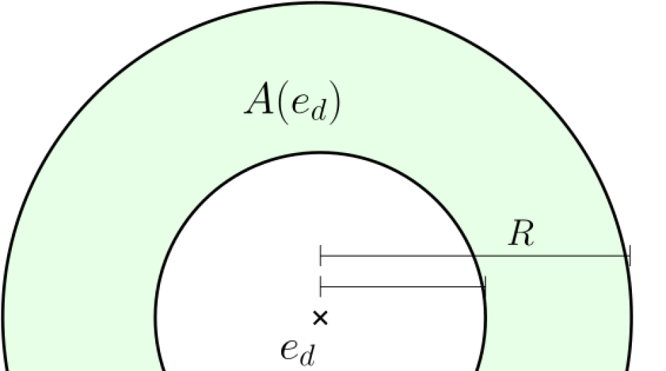
a) $D$ is convex

b) $D$ is $c$-Lipschitz

Figure 1. The set-up for the proof of Theorem 1.1

Take the annulus $A$ from Proposition 2.4. We now consider the two cases:

• $D$ is convex: Up to a rigid motion, we assume that $D\subset H$, where $H=\{(x^{\prime},x_{d}):x_{d}\leq 0\}$. Set

  $$E:=A(e_{d})\cap D,\qquad\partial E=E_{1}\cup E_{2}$$

  where

  $$E_{1}:=\partial D\cap A(e_{d})\subset\partial D\cap B_{1},\qquad E_{2}:=\partial B_{R}(e_{d})\cap D.$$

  Let $v_{1}$ be the (unique) solution from Proposition 2.4 in the annulus $A$. Then for $v(x):=v_{1}(x+e_{d})$, on $E_{1}$,

  $$v(x)\leq 1<2\leq u(x)\quad\text{on}\quad E_{1},$$

  and $v(x)=0$ on $E_{2}$. In particular, we get that

  $$v\leq u\quad\text{on}\quad\partial E.$$

• $\partial D$ is $c$-Lipschitz: Without loss of generality (up to rotation and rescaling), we assume that $D$ is the subgraph/hypograph of a $c$-Lipschitz function $f:B^{d-1}_{2}\to\operatorname{\mathbb{R}}$ in the $e_{d}$ direction and $f(0)=0$ (denote here by $B_{2}^{d-1}$ the $(d-1)$-dimensional ball of radius $2$). Since $f$ is $c$-Lipschitz, we have that for any $0<h<1$ the graph of $f$ lies within $B_{h}^{d-1}\times[-ch,ch]$.

  Then (recall $R\in(1,2)$ is given by Proposition 2.4, so $\frac{R+1}{2}\in(1,R)$), we have

  $$\operatorname{graph}(f)\cap A\left(\frac{R+1}{2}e_{d}\right)\subset B_{2}^{d-1}\times[-2c,2c].$$

  Set now $E$ to be the connected component of

  $$\operatorname{hyp}(f)\cap A\left(\frac{R+1}{2}e_{d}\right)$$

  containing the origin. As long as $c\leq\frac{R-1}{2}$, $\partial E=E_{1}\cup E_{2}$ with

  $$E_{1}\subset\operatorname{graph}(f)\quad\text{ and }\quad E_{2}\subset\partial B_{R}\left(\frac{R+1}{2}e_{d}\right).$$

  Let $v_{1}$ be the solution on the annulus $A$, for

  $$v(x):=v_{1}\left(x+\frac{(R+1)}{2}e_{d}\right)$$

  we have

  $$v(x)\leq 1<2\leq u(x)\qquad\text{ on }E_{1}$$

  and $v(x)=0$ on $E_{2}$. In particular, we get again that

  $$v\leq u\quad\text{on}\quad\partial E.$$

In both cases, we have constructed a set $E$ where the boundary consists of two parts $E_{1}$ and $E_{2}$, and $u|_{E_{1}}>v|_{E_{1}}$ and $u|_{E_{2}}\geq v|_{E_{2}}=0$. Also $v|_{E}$ and $u|_{E}$ are minimizers on $E$ for their own boundary datum, i.e.

$$\operatorname{\textit{F}_{\Lambda}}(v,E)\leq\operatorname{\textit{F}_{\Lambda}}(\min(v,u),E)\qquad\text{and}\qquad\operatorname{\textit{F}_{\Lambda}}(u,E)\leq\operatorname{\textit{F}_{\Lambda}}(\max(v,u),E).$$

From the cut-and-paste lemma for minimizers to the one-phase problem (see [Vel23, Lemma 2.5]),

$$\operatorname{\textit{F}_{\Lambda}}(\min(v,u),E)+\operatorname{\textit{F}_{\Lambda}}(\max(v,u),E)=\operatorname{\textit{F}_{\Lambda}}(v,E)+\operatorname{\textit{F}_{\Lambda}}(u,E),$$

thus $\operatorname{\textit{F}_{\Lambda}}(v,E)=\operatorname{\textit{F}_{\Lambda}}(\min(v,u),E)$. Since $v$ as a minimizer is unique, we have $v=\min(v,u)$, i.e. $u\geq v$ with $v$ vanishing only on a subset of $\partial E$. Hence, there exists some small $\rho>0$ such that on $B_{\rho}\cap D$ the function $u$ is strictly positive as was to be shown. ∎

As a consequence we obtain the proof of the regularity up to the boundary:

Proof of Theorem 1.1.

Assume by contradiction that it is not true. Then there exists $\bar{\varepsilon}>0$ and a sequence $\{g_{k}\}_{k\in\mathbb{N}}$ with $g_{k}\in C(\overline{D})\cap H^{1}(D)$ having a uniform modulus of continuity $\omega$ and $\|g_{k}\|_{H^{1}(D)}\leq M<\infty$ such that for some minimizers $u_{k}$ to (1.2) with $u_{k}-g_{k}=H_{0}^{1}(D)$, there exist $x_{k},y_{k}\in\overline{D}$ such that

(2.1) $$|x_{k}-y_{k}|\leq\frac{1}{k}\to 0\qquad\text{but}\qquad|u_{k}(x_{k})-u_{k}(y_{k})|\geq\bar{\varepsilon}>0,\qquad\text{for}\quad k\in\mathbb{N}.$$

By the uniformity of the modulus of continuity $\omega$ and the boundedness of the $H^{1}$-norm of $g_{k}$, again up to a subsequence $g_{k}\to g_{\infty}$ for some $g_{\infty}$ with the same modulus of continuity $\omega$ and $\|g_{\infty}\|_{H^{1}(D)}\leq M$. Note also that $u_{k}\to u_{\infty}$ in $H^{1}_{loc}(D)$ with $u_{\infty}$ being a minimizer of (1.2) with boundary datum $g_{\infty}$ by [Vel23, Lemma 6.3]. Both, $u_{k}$ and $u_{\infty}$ are locally Lipschitz continuous in $D$ independently of $k$.

Moreover, by compactness of $D$, $x_{k}$ and $y_{k}$ converge, up to a subsequence, to $x_{0}\in\overline{D}$. We now separate between three cases:

Case $x_{0}\in D$: For sufficiently large $k$, $x_{k}$, $y_{k}$, and $x_{0}$ are inside some $D^{\prime}\subset\subset D$. By the interior uniform (Lipschitz) continuity of $u_{k}$ and $u_{\infty}$ we get a contradiction with (2.1).

Case $x_{0}\in\partial D\cap\{g_{\infty}=0\}$: Since $g_{k}\to g_{\infty}$, $g_{k}(x_{0})\to 0$ as well. Consider now the solution to the Dirichlet problem,

$$\left\{\begin{array}[]{rlll}\Delta\bar{u}_{k}&=&0&\text{in }D\\ \bar{u}_{k}&=&g_{k}&\text{on }\partial D.\end{array}\right.$$

By the classical theory ([GT77, Lemma 2.13]), the $\bar{u}_{k}$’s have the same modulus of continuity $\bar{\omega}$, depending only on $\omega$, $d$, $D$ and $M$. Thus

$$|\bar{u}_{k}(x_{k})|\leq|\bar{u}_{k}(x_{k})-\bar{u}_{k}(x_{0})|+|g_{k}(x_{0})|\leq\bar{\omega}(|x_{k}-x_{0}|)+|g_{k}(x_{0})|,$$

which vanishes as $k\to\infty$. Hence $\bar{u}_{k}(x_{k}),\bar{u}_{k}(y_{k})\to 0$. On the other hand, from the subharmonicity of $u_{k}$ , by the comparison principle for weak (sub)solutions we have

$$|u_{k}(x_{k})-u_{k}(y_{k})|\leq u_{k}(x_{k})+u_{k}(y_{k})\leq\bar{u}_{k}(x_{k})+\bar{u}_{k}(y_{k})\to 0,$$

again a contradiction with (2.1).

Case $x_{0}\in\partial D\cap\{g_{\infty}>0\}$: We proceed by using the barrier argument from Lemma 2.5. Without loss of generality, up to a translation, we assume $x_{0}=0$ and observe that for some $\rho>0$ and for any $k$ sufficiently large, $u_{k}>0$ in $B_{\rho}\cap D$, and therefore, the $u_{k}$’s are harmonic there.

Indeed, for $k$ sufficiently large, and up to a rescaling by $r$, $\frac{u_{k}(rx)}{r}$ (independent of $k$), we can assume that $\frac{g_{k}}{r}\geq\frac{g_{\infty}(0)}{2r}$ in $B_{2}\cap\partial D$, so that, up to taking $r$ smaller if necessary (such that $\frac{g_{\infty}(0)}{2r}\geq 2$), we are in the setting of Lemma 2.5. Thus, there is a small $\rho>0$ (independent of $k$) such that $u_{k}>0$ in $D\cap B_{\rho}$, and thereby the $u_{k}$’s are harmonic there. We apply [GT77, Lemma 2.13] to get $u_{k}$ continuous in $\overline{B_{\rho/2}\cap D}$ with a common modulus of continuity $\bar{\omega}$, depending only on $\omega$, $d$, $\rho$, and $D$.

Thus

$$|u_{k}(x_{k})-u_{k}(x_{0})|\leq\bar{\omega}(|x_{k}-x_{0}|),\qquad|u_{k}(y_{k})-u_{k}(x_{0})|\leq\bar{\omega}(|y_{k}-x_{0}|)$$

and therefore, as $k\to\infty$, by the triangle inequality

$$|u_{k}(x_{k})-u_{k}(y_{k})|\leq\bar{\omega}(|x_{k}-x_{0}|)+\bar{\omega}(|y_{k}-x_{0}|)\to 0,$$

again a contradiction to (2.1). This finishes the proof. ∎

2.2. Hölder continuous boundary datum

For the case with Hölder continuous boundary datum, we show that the Hölder regularity is preserved. We do so by following [ESV24]. First we state a well-known technical tool, the Morrey Lemma [Vel23, Lemma 3.12].

Lemma 2.6.

Let $\Omega\subset\operatorname{\mathbb{R}}^{d}$, $u\in H^{1}(\Omega)$ and for $C>0$, $\gamma\in(-1,1)$

$$\fint_{B_{r}(x_{0})}|\nabla u|^{2}dx\leq C^{2}r^{2(\gamma-1)}\qquad\forall x_{0}\in B_{R/8}\quad\forall r\leq\frac{R}{2}.$$

Then $u\in C^{0,\gamma}(B_{R/8})$ with

$$\|u\|_{C^{0,\gamma}(B_{R/8})}\leq C\left(2^{d}+\frac{2}{\gamma}\right).$$

We now can prove the local version of Proposition 1.2:

Proposition 2.7.

Let $D$ be an open bounded $C^{1,\alpha}$ domain in $B_{1}$, given by the subgraph of a function with $C^{1,\alpha}$ norm bounded by 1. Let $u$ be a minimizer of (1.2) on $D$ with boundary datum $g\in C^{\gamma}(\bar{D})\cap H^{1}(D)$ with $1>\gamma>\frac{1}{2}$, and $0\in\partial\{u>0\}$. Then,

$$\|u\|_{C^{\gamma}(B_{1/2}\cap\overline{D})}\leq C\left(\|u\|_{C^{\gamma}(B_{1}\cap\partial D)}+\|u\|_{L^{\infty}(B_{1}\cap D)}+1\right),$$

for some constant $C$ depending only on $d$, $\gamma$, and $\alpha$.

Proof.

Let $\partial D$ be the graph of a $C^{1,\alpha}$ function $\phi$ in $B_{1}$, i.e. $\partial D\cap B_{1}=\{(x^{\prime},\phi(x^{\prime})):x^{\prime}\in\operatorname{\mathbb{R}}^{d-1}\}$. It suffices to show $\gamma$-Hölder continuity in a small ball $B_{1/8}$. Denote the positive and negative half spaces by $H^{+}$ and $H^{-}$.

First, we extend $\nabla u:B_{1}\cap D\to\operatorname{\mathbb{R}}^{d}$ to $\nabla u:B_{1}\to\operatorname{\mathbb{R}}^{d}$. In order to do so, let $\Phi:B_{1}\to\operatorname{\mathbb{R}}^{d}$ be the $C^{1,\alpha}$ function

$$\Phi(x^{\prime},x_{d}):=(x^{\prime},x_{d}+g(x^{\prime})).$$

Up to translation and rotation, we assume $\Phi(0)=0$ and $D\Phi(0)=I_{d\times d}$. Let

$$\pi:(y^{\prime},y_{d})\mapsto(y^{\prime},-y_{d}),$$

we define the extension

$$\nabla u(x)=\begin{cases}\nabla u(x)\qquad&\text{if }x\in D\cap B_{1},\\ \nabla u(\Phi\circ\pi\circ\Phi^{-1}(x))\qquad&\text{if }x\in D^{c}\cap B_{1}.\end{cases}$$

The idea is to arrive at an estimate for $u$ of the form

(2.2) $$\forall\bar{x}\in B_{1/8},\forall r\leq\frac{1}{2}:\qquad\int_{B_{r}(\bar{x})}|\nabla u|^{2}\leq Cr^{d+2(\gamma-1)},$$

and then use the Morrey Lemma [Vel23, Lemma 3.12], which gives directly $\gamma$-Hölder regularity in $B_{1/8}$. As in [ESV24], it suffices to show the estimate on the boundary, i.e. for a fixed $r>0$ small enough and $x_{0}\in\partial D\cap B_{1/8}$,

(2.3) $$\int_{B_{r}(x_{0})}|\nabla u|^{2}\leq Cr^{d+2(\gamma-1)}.$$

By a translation, we assume that $x_{0}=0$. Performing the change of variable,

$$x=\Phi(y),\qquad dx=|D\Phi(y)|dy,$$

we have

$$\begin{split}&\int_{B_{r}}|\nabla u(x)|^{2}dx=\int_{\Phi(B_{r})}|\nabla u(x)|^{2}dx=\int_{B_{r}}|\nabla u(\Phi(y))|^{2}|D\Phi(y)|dy\\ &\qquad=\int_{B_{r}\cap H^{+}}|\nabla u(\Phi(y))|^{2}|D\Phi(y)|dy+\int_{B_{r}\cap H^{-}}|\nabla u(\Phi\circ\pi\circ\Phi^{-1}(\Phi(y)))|^{2}|D\Phi(y)|dy\\ &\qquad=2\int_{B_{r}\cap H^{+}}|\nabla u(\Phi(y))|^{2}|D\Phi(y)|dy=2\int_{\Phi(H^{+}\cap B_{r})}|\nabla u(x)|^{2}dx.\end{split}$$

Step 1: Let $h_{g}:H^{+}\cap B_{1}\to\operatorname{\mathbb{R}}$ such that

$$\left\{\begin{array}[]{rlll}\Delta h_{g}&=&0&\text{in }H^{+}\cap B_{1},\\ h_{g}&=&g\circ\Phi&\text{ on }\partial(H^{+}\cap B_{1}),\end{array}\right.$$

which is in $C^{\gamma}(\bar{H}^{+}\cap B_{1/2})$ by [MS06, Proposition 2.1] ($u$ is continuous in $\overline{D}$ by Theorem 1.1) with

$$\begin{split}\|h_{g}\|_{C^{\gamma}(H^{+}\cap B_{1/2})}&\leq C_{d,\gamma}\left(\|g\circ\Phi\|_{C^{\gamma}(H^{+}\cap B_{1})}+\|h_{g}\|_{L^{\infty}(\partial H^{+}\cap B_{1})}\right)\\ &\leq C\left(\|g\|_{C^{\gamma}(\partial D)}+\|g\|_{L^{\infty}(H^{+}\cap B_{1})}\right),\end{split}$$

for $C$ depending on $d,\gamma$ and the $C^{1,\alpha}$ norm of $D$. We now claim that inside $H^{+}\cap B_{1/2}$

$$|\nabla h_{g}(x)|\leq C_{d}\|h_{g}\|_{C^{\gamma}(H^{+}\cap B_{1/2})}\operatorname{dist}(x,\partial H^{+})^{\gamma-1}.$$

For a fixed $x$, Take $x_{1}\in\partial H^{+}$ such that $|x-x_{1}|=\operatorname{dist}(x,\partial H^{+})=:\delta(x)$ and let

$$v(x)\coloneq h_{g}(x)-h_{g}(x_{1}).$$

By $\gamma$-Hölder regularity of $v$, from the definition, for $x\in H^{+}\cap B_{1/2}$

$$v(x)=v(x_{1})+R(x)=R(x)\qquad\text{with }|R(x)|\leq 2\|h_{g}\|_{C^{\gamma}(H^{+}\cap B_{1/2})}|x-x_{1}|^{\gamma}.$$

By standard harmonic estimates,

$$\begin{split}|\nabla h_{g}(x)|=|\nabla v(x)|&\leq\sup_{B_{\delta(x)/4}(x)}|\nabla v(y)|\\ &\leq\frac{d}{\delta(x)}\sup_{B_{\delta(x)/2}(x)}|v(y)|\\ &\leq\frac{d}{\delta(x)}\sup_{B_{\delta(x)/2}(x)}|R(y)|\\ &\leq\frac{2d\|h_{g}\|_{C^{\gamma}(H^{+}\cap B_{1/2})}}{\delta(x)}\sup_{B_{\delta(x)/2}(x)}|y-x_{1}|^{\gamma}\\ &\leq 4d\|h_{g}\|_{C^{\gamma}(H^{+}\cap B_{1/2})}\delta(x)^{\gamma-1},\end{split}$$

proving the claim. In the co-area formula [Fed69, Theorem 3.2.22], take $f(x)=\delta(x)$ and $g(x)=\delta(x)^{2(\alpha-1)}$. Since $\partial H^{+}=\{x_{d}=0\}$ we have $|\nabla f(x)|=1$. Hence, as

$$f^{-1}(t)=\{x\in H^{+}\cap B_{r}:\delta(x)=t\},$$

we estimate for $r<\frac{1}{2}$,

$$\begin{split}\int_{H^{+}\cap B_{r}}|\nabla h_{g}|^{2}dx&\leq C_{d}\|h_{g}\|^{2}_{C^{\gamma}(H^{+}\cap B_{1/2})}\int_{H^{+}\cap B_{r}}\delta(x)^{2(\gamma-1)}dx\\ &=C_{d}\|h_{g}\|^{2}_{C^{\gamma}(H^{+}\cap B_{1/2})}\int_{H^{+}\cap B_{r}}\delta(x)^{2(\gamma-1)}|\nabla f|dx\\ &=C_{d}\|h_{g}\|^{2}_{C^{\gamma}(H^{+}\cap B_{1/2})}\int_{\operatorname{\mathbb{R}}}\int_{\{x\in H^{+}\cap B_{r}:\delta(x)=t\}}\delta(x)^{2(\gamma-1)}d\operatorname{\mathcal{H}}^{d-1}(x)dt\\ &=C_{d}\|h_{g}\|^{2}_{C^{\gamma}(H^{+}\cap B_{1/2})}\int_{\operatorname{\mathbb{R}}}t^{2(\gamma-1)}\operatorname{\mathcal{H}}^{d-1}(\{x\in H^{+}\cap B_{r}:\delta(x)=t\})dt\\ &=C_{d}\|h_{g}\|^{2}_{C^{\gamma}(H^{+}\cap B_{1/2})}\int_{0}^{r}t^{2(\gamma-1)}\operatorname{\mathcal{H}}^{d-1}(\{x\in H^{+}\cap B_{r}:\delta(x)=t\})dt\\ &\leq C_{d}\|h_{g}\|^{2}_{C^{\gamma}(H^{+}\cap B_{1/2})}r^{d-1}\int_{0}^{r}t^{2(\gamma-1)}dt\\ &=C_{d}\|h_{g}\|^{2}_{C^{\gamma}(H^{+}\cap B_{1/2})}r^{d+2(\gamma-1)}.\end{split}$$

The rest of the proof follows exactly as in [ESV24], with the constant only depending on $d$, $\gamma$ and the $C^{1,\alpha}$ norm of $D$, but not on the Hölder norm of $g$. (We remark that $g$ here is named $\varphi$ in [Vel23].) We thereby conclude that (2.2) is satisfied since

$$\int_{B_{r}(x_{0})}|\nabla u|^{2}\leq C\|h_{g}\|^{2}_{C^{\gamma}(H^{+}\cap B_{1/2})}r^{d+2(\gamma-1)},$$

and thus by Lemma 2.6, the analogous interior regularity estimate, and the bound for $\|h_{g}\|_{C^{\gamma}(H^{+}\cap B_{1/2})}$, we have that $u$ is locally $C^{\gamma}$ Hölder continuous with

$$\|u\|_{C^{\gamma}(B_{1/8}\cap\overline{D})}\leq C\left(\|u\|_{C^{\gamma}(B_{1}(x_{0})\cap\partial D)}+\|u\|_{L^{\infty}(B_{1}(x_{0})\cap D))}+1\right),$$

as we wanted to show. ∎

As a consequence, we obtain directly Proposition 1.2.

Proof of Proposition 1.2.

Since $D$ is bounded and a $C^{1,\alpha}$ domain, up to a rescaling we can pick $x_{1},...,x_{N}\in\partial D$ such that $\partial D\subset\bigcup_{i=1}^{N}B_{1/2}(x_{i})=:S$ and inside each $B_{1}(x_{i})$ we are in the setting of Proposition 2.7. Thus by Proposition 2.7,

$$\begin{split}\|u\|_{C^{\gamma}(S)}&\leq\sum_{i=1}^{N}\|u\|_{C^{\gamma}(B_{1/2}(x_{i})\cap\overline{D})}\\ &\leq\sum_{i=1}^{N}C\left(\|u\|_{C^{\gamma}(B_{1}(x_{i})\cap\partial D)}+\|u\|_{L^{\infty}(B_{1}(x_{i})\cap D))}+1\right)\\ &\leq C\left(\|g\|_{C^{\gamma}(\partial D)}+\|u\|_{L^{\infty}(D)}+1\right).\end{split}$$

Since $u$ is Lipschitz continuous on $D\backslash S\subset\subset D$ with

$$\|\nabla u\|_{L^{\infty}(D\backslash S)}\leq C\left(1+\frac{\|u\|_{L^{\infty}(D)}}{\operatorname{dist}^{d+1}(D\backslash S,\partial D)}\right),$$

the result follows. ∎

Remark 2.8.

For $\gamma<\frac{1}{2}$, it is not a priori given that the boundary datum $g$ is the trace of a function in $H^{1}(D)$. For $\gamma\leq\frac{1}{2}$ and $g\in C^{\gamma}(\bar{D})\cap H^{1}(D)$, the previous proof does not work, since we crucially use the minimality if $u$.

Remark 2.9.

If $\gamma=1$ (i.e. the datum is Lipschitz), then using the same argument as above we recover the result from [ESV24], as expected,

$$\forall x_{0}\in\overline{\Omega}\cap B_{1/2},r\leq\frac{1}{2}:\qquad\fint_{B_{r}(x_{0})}|\nabla u|^{2}\leq Cr^{d+2(\gamma-1)},\qquad\forall\gamma<1.$$

This implies local $\gamma$-Hölder regularity for any $\gamma<1$, but not Lipschitz regularity, in the exact same fashion as for the Laplace equation with Dirichlet boundary condition. It remains open whether this result could be improved to show e.g. $\log$-Lipschitz continuity of the solution,

$$|u(x)-u(y)|\leq C|\log|x-y||\cdot|x-y|\qquad\forall x,y\in\overline{D}.$$

3. Applications of boundary regularity

3.1. Generic uniqueness of minimizers

Since the functional $\operatorname{\textit{F}_{\Lambda}}$ is not convex, in general, there is no reason to expect uniqueness of minimizers. Already in one dimension it is possible to construct a boundary datum $g$ giving two nonidentical minimizers. However, the cases with several minimizers are rare and we expect “almost everywhere” a unique minimizer. We start with a general comparison principle, which can be applied to many different contexts.

Lemma 3.1.

Let $D$ be a bounded open domain of $\operatorname{\mathbb{R}}^{d}$, and let $g,g^{\prime}\in C(\overline{D})\cap H^{1}(D)$ with $g^{\prime}\geq g\geq 0$ in $D$ and $g^{\prime}(z)>g(z)>0$ at some $z$ in each connected component of $\partial D\cap\{g>0\}$. Then for corresponding minimizers to (1.2), $u_{g}$ and $u_{g^{\prime}}$, we have $u_{g^{\prime}}\geq u_{g}$ on $\overline{D}$.

Proof.

Since on $\{u_{g}=0\}$ the result holds trivially, consider the open set $\Omega_{u_{g}}=\{u_{g}>0\}\cap D$.

Define $\tilde{u}(x)\coloneq\max\left\{u_{g^{\prime}}(x),u_{g}(x)\right\}$. Since by a computation ([Vel23, Lemma 2.5])

$$\operatorname{\textit{F}_{\Lambda}}(\max\{u_{g^{\prime}},u_{g}\},D)+\operatorname{\textit{F}_{\Lambda}}(\min\{u_{g^{\prime}},u_{g}\},D)=\operatorname{\textit{F}_{\Lambda}}(u_{g^{\prime}},D)+\operatorname{\textit{F}_{\Lambda}}(u_{g},D),$$

we have that $\tilde{u}$ is also a minimizer with $\Delta\tilde{u}=0$ in $\Omega_{u_{g}}\subset\Omega_{\tilde{u}}$. Suppose for contradiction that there exists $x_{0}\in\Omega_{u_{g}}$ such that $u_{g}(x_{0})>u_{g^{\prime}}(x_{0})$, that is $\tilde{u}(x_{0})=u_{g}(x_{0})$. Let $\mathcal{C}$ be the connected component of $\Omega_{u_{g}}$ containing $x_{0}$.

Set $h(x)\coloneq\tilde{u}(x)-u_{g}(x)\geq 0$, then on $\mathcal{C}$, $\Delta h=0$ and as its minimum value of $0$ is attained at $x_{0}\in\mathcal{C}$, by the strong maximum principle $h\equiv 0$ and $\tilde{u}=u_{g}$ on $\overline{\mathcal{C}}$.

We now show for the sake of contradiction that $\overline{\mathcal{C}}$ contains boundary points where $\tilde{u}>u_{g}>0$. If $\partial\mathcal{C}\subset\{u_{g}=0\}$, then by the maximum principle, $u\equiv 0$ in $\mathcal{C}$, contradicting $\mathcal{C}\subset\Omega_{u_{g}}$. Hence $\partial\mathcal{C}\cap\Omega_{u_{g}}\neq\varnothing$. Let $x_{1}\in\partial\mathcal{C}\cap\Omega_{u_{g}}$, if $x_{1}\in\textnormal{int}(D)$, then by interior Lipschitz continuity $x_{1}$ cannot be a point in $\partial C$, i.e. $x_{1}\in\partial D$ with $g(x_{1})>0$. Now the whole component $\partial D\cap\{g>0\}$ containing $x_{1}$ is contained in $\partial\mathcal{C}$ by continuity from Theorem 1.1. But by assumption we have $z\in\bar{C}$ with

$$\tilde{u}(z)\geq u_{g^{\prime}}(z)=g^{\prime}(z)>g(z)=u_{g}(z),$$

a contradiction to the fact that $\tilde{u}=u_{g}$ on $\mathcal{C}$, finishing the proof. ∎

We are now able to prove the generic uniqueness for the one-phase problem, using the argument from [FY23, Proposition 1.2], but for a wider class of boundary data.

Proof of Proposition 1.3.

During the proof we again use the Lipschitz continuity of minimizers, and we recall that we are taking $\Lambda=1$. By Lemma 3.1, minimizers are ordered with respect to the boundary datum, i.e. $t^{\prime}>t>0$ implies that $u_{t^{\prime}}\geq u_{t}$.

Let $t$ be such that there are at least two distinct minimizers $u_{t}^{1},u_{t}^{2}$. Let $u_{t}^{+}=\max\{u_{t}^{1},u_{t}^{2}\}$ and $u_{t}^{-}=\min\{u_{t}^{1},u_{t}^{2}\}$, then

$$\begin{split}\operatorname{\textit{F}_{\Lambda}}(u_{t}^{+})+\operatorname{\textit{F}_{\Lambda}}(u_{t}^{-})&=\int_{D\cap\{u_{t}^{1}\geq u_{t}^{2}\}}|\nabla u_{t}^{1}|^{2}+\int_{D\cap\{u_{t}^{1}<u_{t}^{2}\}}|\nabla u_{t}^{2}|^{2}\\ &\quad+|(\{u_{t}^{1}>0\}\cup\{u_{t}^{2}>0\})\cap D|\\ &\quad+\int_{D\cap\{u_{t}^{1}\geq u_{t}^{2}\}}|\nabla u_{t}^{2}|^{2}+\int_{D\cap\{u_{t}^{1}<u_{t}^{2}\}}|\nabla u_{t}^{1}|^{2}\\ \ &\quad+|\{u_{t}^{1}>0\}\cap\{u_{t}^{2}>0\}\cap D|\\ &=\operatorname{\textit{F}_{\Lambda}}(u_{t}^{1})+\operatorname{\textit{F}_{\Lambda}}(u_{t}^{2}).\end{split}$$

As $u_{t}^{1}$ and $u_{t}^{2}$ are minimizers, so are $u_{t}^{+}$ and $u_{t}^{-}$. Now let $x_{0}$ be a point where $u_{t}^{1}$ and $u_{t}^{2}$ differ, i.e. without loss of generality $u_{t}^{1}(x_{0})-u_{t}^{2}(x_{0})=\varepsilon$. By Lipschitz continuity, there exists $B_{r}(x_{0})$ where $u_{t}^{1}(x_{0})-u_{t}^{2}(x_{0})>\varepsilon/2$. Thus for $\rho=\min\{\varepsilon/3,r\}$, there exists a $d+1$ dimensional ball $B_{\rho}$ such that $B_{\rho}\subset\textrm{epi}(u_{t}^{2})\backslash\textrm{epi}(u_{t}^{1})$.

Repeating the argument for any $t$ with non-unique minimizers gives a collection of disjoint (as minimizers are ordered with respect to the boundary datum) balls. Since there can be at most countably many disjoint open balls in $\operatorname{\mathbb{R}}^{d}$, the proof is finished. ∎

3.2. Generic regularity of the free boundary

We now prove a slightly weaker version of Theorem 1.4, namely, the case where the boundary data is equicontinuous. The main part is already done in [FY23, Section 4], it remains only to prove [FY23, Lemma 4.3] for the larger class of boundary data (i.e. equicontinuous, which then implies the result for continuous data, see Lemma 3.3) instead of equi-Lipschitz).

Proposition 3.2.

Theorem 1.4 holds under the added assumption that the family $g_{t}$ is equicontinuous.

Proof.

For simplicity of the exposition, we assume that $D=B_{1}$. Fix $\tau\in(0,1)$ and let $x_{0}$ be a free boundary point, $x_{0}\in B_{1/2}\cap\partial\Omega_{u_{t_{0}}}$. for some $t_{0}\in[\tau,1)$. In view of [FY23, Lemma 4.3], we need to show that there exists $\kappa=\kappa(\tau,d,\omega,M)>0$ (with $\omega$ the common modulus of continuity of $\{g_{t}\}$ and $M$ its uniform $H^{1}$ bound), such that

$$\sup_{B_{\kappa(t-t_{0})}(x)}u_{t_{0}}\leq u_{t}(x)\qquad\text{for }x\in B_{3/4}\text{ and }t\in[t_{0},1).$$

By the assumptions on $\{g_{t}\}$, we have

$$g_{t_{0}}\geq\tau>0\qquad\text{ on }\partial B_{1}.$$

Applying now Theorem 1.1 ($u_{t_{0}}$ is continuous up to the boundary with modulus of continuity $\bar{\omega}(d,\omega,M)$), gives $\delta=\delta(\tau,d,\omega,M)<1/16$ such that

$$u_{t_{0}}>0\qquad\text{in }U:=B_{1}\backslash\overline{B_{1-8\delta}}.$$

Using now the comparison lemma, Lemma 3.1, gives $u_{t}\geq u_{t_{0}}$ for $t\geq t_{0}$ and as $U\subset\Omega_{u_{t_{0}}}\subset\Omega_{u_{t}}$,

$$\Delta(u_{t}-u_{t_{0}})=0\qquad\text{in }U.$$

The rest of the proof follows analogously to [FY23, Lemma 4.3]. ∎

We set out to remove the assumption of equicontinuity in the previous statement. The rough idea is to partition a family of continuous (not necessarily equicontinuous) functions into countable subfamilies of equicontinuous functions, apply Theorem 3.2 on each subfamily and then show that the size of the set of functions not falling into any equicontinuous subfamily is small. This is due to the separability of continuous functions.

Lemma 3.3.

Let $d\geq 1$ and $D\subset\operatorname{\mathbb{R}}^{d}$ a bounded Lipschitz domain. Let $\{g_{t}\}_{t\in(0,1)}$ be a monotone family of continuous functions in $\overline{D}$, i.e.

$$t\geq s\quad\implies\quad g_{t}\geq g_{s}\quad\text{in}\quad\overline{D}.$$

Then, there exists a countable family of disjoint open intervals $\{I_{k}\}_{k\in\mathbb{N}}$ with $I_{k}\subset(0,1)$ such that

• $(0,1)\setminus\bigcup_{k\in\mathbb{N}}I_{k}$ is countable,

• $g_{t}$ are locally equicontinuous for $t\in I_{k}$. That is, for any $K\subset I_{k}$ compact, the family $\{g_{t}\}_{t\in K}$ is equicontinuous.

Proof.

Let $T\subset(0,1)$ be the set where $\{g_{t}\}_{t\in(0,1)}$ is locally equicontinuous, i.e.

$$T:=\{t\in(0,1):\quad\exists\eta>0\text{ s.t. }\{g_{s}\}_{(t-\eta,t+\eta)}\text{ is equicontinuous}\}.$$

Since for $t_{0}\in T$ and $t\in B_{\eta/2}(t_{0})$ (where $\eta=\eta(t_{0})$),

$$\{g_{s}\}_{(t-\eta/2,t+\eta/2)}\subset\{g_{s}\}_{(t_{0}-\eta,t_{0}+\eta)},$$

it follows that $T$ is open in $(\{g_{s}\}_{(0,1)},\|\cdot\|_{L^{\infty}(D)})$. Next, we show by contraposition that for a fixed $t\in T^{c}$, either

$$\exists\varepsilon>0:\inf_{s>t}\|g_{t}-g_{s}\|_{L^{\infty}(D)}\geq\varepsilon\quad\text{ or }\quad\exists\varepsilon>0:\inf_{s<t}\|g_{t}-g_{s}\|_{L^{\infty}(D)}\geq\varepsilon.$$

Indeed, suppose it is not true true. Since $\{g_{s}\}_{(0,1)}$ is monotone, we have

$$\begin{split}\forall\varepsilon>0,\,&\inf_{s>t}\|g_{t}-g_{s}\|_{L^{\infty}(D)}<\varepsilon\quad\text{ and }\quad\forall\varepsilon>0,\,\inf_{s<t}\|g_{t}-g_{s}\|_{L^{\infty}(D)}<\varepsilon\\ \end{split}$$

that is,

$$\lim_{s\to t}\|g_{t}-g_{s}\|_{L^{\infty}(D)}=0.$$

Let $\varepsilon>0$ and take $\eta,\delta>0$ such that

$$\begin{split}|s-t|<\eta&\implies\|g_{t}-g_{s}\|_{L^{\infty}(D)}<\frac{\varepsilon}{3},\\ |x-y|<\delta&\implies|g_{t}(x)-g_{t}(y)|<\frac{\varepsilon}{3}.\end{split}$$

By the triangle inequality,

$$|g_{s}(x)-g_{s}(y)|\leq|g_{s}(x)-g_{t}(x)|+|g_{t}(x)-g_{t}(y)|+|g_{t}(y)-g_{s}(y)|\leq\varepsilon,$$

it follows that $\{g_{s}\}_{(t-\eta,t+\eta)}$ is equicontinuous, as $\delta$ does not depend on $s$, giving a contradiction.

It remains to show that $T^{c}$ is countable. We have

$$T^{c}=\underbrace{\{t\in(0,1):\inf_{s>t}\|g_{t}-g_{s}\|_{L^{\infty}(D)}>0\}}_{=:T^{c}_{1}}\cup\underbrace{\{t\in(0,1):\inf_{s<t}\|g_{t}-g_{s}\|_{L^{\infty}(D)}>0\}}_{=:T^{c}_{2}}.$$

Let

$$J_{m}:=\{t\in(0,1):\inf_{s>t}\|g_{t}-g_{s}\|_{L^{\infty}(D)}\geq\tfrac{1}{m}\},\quad\text{for}\quad m\in\mathbb{N}.$$

Then, by definition, we have

$$T_{1}^{c}=\bigcup_{m\in\mathbb{N}}J_{m}.$$

For any $m\in\mathbb{N}$ and $t_{1},t_{2}\in J_{m}$ with $t_{2}\neq t_{1}$ we have $\|g_{t_{1}}-g_{t_{2}}\|_{L^{\infty}(D)}\geq\tfrac{1}{m}>0$, and so the family $\{g_{t}\}_{t\in J_{m}}$ is a family of continuous functions that are pairwise at distance $\tfrac{1}{m}$. However, $C(\bar{D})$ and then also $\{g_{t}\}_{t\in J_{m}}$ are separable, that is, there exists a countable subset $I\subset J_{m}$ such that $\{g_{t}\}_{t\in I}$ is dense in $\{g_{t}\}_{t\in J_{m}}$. Take $g_{t}\in\{g_{t}\}_{t\in J_{m}}$ and $t_{n}\in I\subset J_{m}$ with $\|g_{t_{n}}-g_{t}\|_{L^{\infty}(D)}\to 0$. The lower bound on the pairwise distance implies that $t_{n}=t$ for all $n$ large enough, i.e. for any $t\in J_{m}$, $g_{t}\in\{g_{t}\}_{t\in I}$, thus $J_{m}$ is countable. Since $m$ was arbitrary and countability is preserved under countable unions, $T^{c}_{1}$ is countable and by the same argument $T^{c}_{2}$ is countable as well, and so is $T^{c}$.

Since $T\subset(0,1)$ is open it can be written as a disjoint union of open intervals, that is $(0,1)=T^{c}\cup T=T^{c}\cup\bigcup_{k\in\mathbb{N}}I_{k}$. Now, $K\subset\subset I_{k}$, $\{(t-\eta_{t},t+\eta_{t}\}_{t\in K}$ admits a finite subcover; and we take as common modulus of continuity its maximum. ∎

We now combine Proposition 3.2 with Lemma 3.3 to obtain the generic regularity result for a general (not necessarily equicontinuous) family of continuous boundary data, thus proving Theorem 1.4 in its full generality.

Proof of Theorem 1.4.

We first treat the case $d=d^{*}+1$. By Lemma 3.3, let $J_{0}=(0,1)\setminus\bigcup_{k\in\mathbb{N}}I_{k}$ and $\{g_{s}\}_{s}$ locally equicontinuous for $s\in I_{k}$ for each $k$. By taking a countable compact exhaustion of $I_{k}$ and applying Theorem 3.2 in each compact, we deduce that, for each $k$, there is $J_{k}$ countable such that $\textnormal{Sing}(u_{t})=\varnothing$ on $I_{k}\backslash J_{k}$. The result follows by setting $J:=J_{0}\cup\bigcup_{k\in\mathbb{N}}J_{k}$.

For the case $d\geq d^{*}+2$, since the dimension estimate $\dim_{\operatorname{\mathcal{H}}}\textnormal{Sing}(u_{t})\leq d-d^{*}-2$ holds for almost every $t\in K$ and every $K\subset\subset I_{k}$, it holds a.e. on $I_{k}$. Hence it holds also almost everywhere on $(0,1)$. ∎

References

- [AC81] H. Alt and L. Caffarelli “Existence and regularity for a minimum problem with free boundary.” In Journal für die reine und angewandte Mathematik 325, 1981, pp. 105–144
- [ACF82] H. Alt, L. Caffarelli and A. Friedman “Jet flows with gravity” In Journal für die reine und angewandte Mathematik 1982.331, 1982, pp. 58–103
- [BL82] J. Buckmaster and G. Ludford “Theory of Laminar Flames”, Cambridge Monographs on Mechanics Cambridge University Press, 1982
- [Caf77] L. Caffarelli “The regularity of free boundaries in higher dimensions” In Acta Mathematica 139 Institut Mittag-Leffler, 1977, pp. 155–184
- [CS05] L. Caffarelli and S. Salsa “A Geometric Approach to Free Boundary Problems”, Graduate studies in mathematics American Mathematical Society, 2005
- [EFY23] M. Engelstein, X. Fernández-Real and H. Yu “Graphical solutions to one-phase free boundary problems” In Journal für die reine und angewandte Mathematik 804, 2023, pp. 155–195
- [ESV20] M. Engelstein, L. Spolaor and B. Velichkov “Uniqueness of the blowup at isolated singularities for the Alt–Caffarelli functional” In Duke Mathematical Journal 169.8 Duke University Press, 2020, pp. 1541–1601
- [ESV24] Nick Edelen, Luca Spolaor and Bozhidar Velichkov “A strong maximum principle for minimizers of the one-phase Bernoulli problem” In Indiana Univ. Math. J. 73, 2024, pp. 1061–1096
- [Fed69] H. Federer “Geometric Measure Theory”, Classics in Mathematics Springer, 1969
- [FY23] X. Fernández-Real and H. Yu “Generic properties in free boundary problems” In arXiv: 2308.13209, 2023
- [GT77] D. Gilbarg and N. Trudinger “Elliptic Partial Differential Equations of Second Order”, Classics in Mathematics Springer, 1977
- [JS14] D. Jerison and O. Savin “Some remarks on stability of cones for the one-phase free boundary problem” In Geometric and Functional Analysis 25, 2014, pp. 1240–1257
- [MS06] E. Milakis and L. Silvestre “Regularity for Fully Nonlinear Elliptic Equations with Neumann Boundary Data” In Communications in Partial Differential Equations 31, 2006, pp. 1227–1252
- [Vel23] B. Velichkov “Regularity of the One-phase Free Boundaries”, Lecture Notes of the Unione Mathematica Italiana Springer, 2023
- [Wei99] G. Weiss “Partial regularity for a minimum problem with free boundary” In The Journal of Geometric Analysis 9, 1999, pp. 317–326