Relaxing towards generalized one-body Boltzmann states

Abstract

Isolated quantum systems follow the reversible unitary evolution; if we focus on the dynamics of local states and observables, they exhibit the irreversible relaxation behaviors. Here we study the local relaxation process in an isolated chain consisting of N three level systems. Though the entropy of the full many body state keeps a constant, it turns out the total correlation of this system approximately exhibits a monotonically increasing behavior. More importantly, a variation analysis shows that, the total correlation entropy would achieve its theoretical maximum when each site stays in a generalized one-body Boltzmann state, which is not solely determined by the energy but also depends on the spin value of each onsite level. It turns out such a theoretical correlation maximum is highly coincident with the result obtained from the exact time dependent evolution. In this sense, the total correlation entropy well serves as an indicator for the dynamical irreversibility of the nonequilibrium relaxation in this isolated system.

Introduction - Open systems would be thermalized to be a thermal state having the same temperature with its reservoir. However, the thermalization process for isolated many body systems is tricky to define [1, 2], since the reversible unitary/Liouville dynamics guarantees the entropy of isolated quantum/classical systems never changes [3, 4, 5].

For an isolate gas with weak particle collisions, focusing on the one-particle probability distribution function (PDF), Boltzmann derived a transport equation and proved that the entropy of this one-particle PDF always increases until it finally reaches the Boltzmann-Maxwell distribution (the Boltzmann H-theorem) [6, 4, 7].

Regardless of the dynamical process, focusing on the observable expectations in the equilibrium state long after relaxation, the ensemble theory was established based on the statistics interpretation, which forms the foundation of statistical physics [8, 9, 10].

To understand the connection between the reversible microscopic dynamics and the statistical ensemble descriptions, the eigenstate thermalization hypothesis (ETH) provides an inspiring sight [11, 12, 13, 14, 10, 15]. Based on the ergodicity hypothesis, the state of long time average is considered (diagonal ensemble [16]),

$$\bar{\boldsymbol{\rho}}_{\text{{d}}}\equiv\lim_{T\rightarrow\infty}\frac{1}{T}\int_{0}^{T}dt\,\hat{\boldsymbol{\rho}}(t)=\sum P_{k}\,|E_{k}\rangle\langle E_{k}|.$$ (1)

Here $\big{\{}|E_{k}\rangle\big{\}}$ are the eigenstates of the full isolated many body system, and the probabilities $P_{k}$ are determined by the initial state. Generally, $\bar{\boldsymbol{\rho}}_{\text{{d}}}$ is not identical to the microcanonical ensemble $\hat{\boldsymbol{\rho}}_{\text{mc}}$, but many numerical studies show that, for a wide class of few body observables $\hat{o}$, these two states give almost identical expectations, i.e., $\mathrm{tr}[\bar{\boldsymbol{\rho}}_{\text{{d}}}\hat{o}]\simeq\mathrm{tr}[\hat{\boldsymbol{\rho}}_{\text{mc}}\hat{o}]$ (for nonintegrable systems). In this sense, effectively this isolated system is said to achieve thermalization [16, 17].

For integrable systems, $\bar{\boldsymbol{\rho}}_{\text{{d}}}$ does not coincide with the microcanonical ensemble $\hat{\boldsymbol{\rho}}_{\text{mc}}$, but with a generalized Gibbs ensemble $\hat{\boldsymbol{\rho}}_{\text{{gge}}}\sim\exp(-\sum\,\lambda_{m}\,\hat{\mathcal{I}}_{m})$ [18], where $\{\hat{\mathcal{I}}_{m}\}$ is the full set of the integrals of motion. In disordered systems with many body localization [19, 20, 21, 22, 23], as well as some other systems with nonergodic properties [24, 25, 26, 27, 28, 29, 30, 31], features seemingly defying ETH have been found [16, 17].

It is worth noting that the long-time averaging plays an essential role in the above thermalization definition. For the dynamical relaxation process, it remains desirable to find out a quantity that is capable to to describe the irreversible entropy increase as in the standard thermodynamics, and to understand the transition how the deterministic reversible evolutions in few body systems become irreversible relaxations with the increase of the system size.

For this purpose, in analogy to Boltzmann’s discussions on the isolate gas [6, 4], we focus on the time dependent evolution of the one-body states and the associated observable expectations (local relaxation [32, 33, 34, 35, 36]), and study their relaxation processes in a finite chain of $N$ three-level systems. We find that, though the total $N$-body state experiences the deterministic unitary evolution, the local observable expectations exhibit irreversible relaxation behaviors, namely, they first approach certain values as their steady states and then experience small fluctuations around them [37]. Besides, for a finite size, hierarchy recurrences (revivals) appear periodically, which can be explained by the propagation of local excitation patterns [38, 39, 40, 41].

Though the entropy of the full $N$-body state keeps a constant, we find that the total correlation entropy [42, 43, 44, 45] in this system approximately exhibits a monotonically increasing behavior similar to that in the standard thermodynamics [46, 47, 48, 49, 50, 51, 52, 39, 40]. We calculate the possible maximum of the total correlation entropy by variation under proper constraints, and find that the theoretical maximum is achieved when each individual site is in a generalized one-body Boltzmann state (GOBBS), i.e., $\tilde{\varrho}_{n}\sim\exp(-\beta_{\text{{e}}}\hat{H}_{n}-\beta_{\text{{s}}}\hat{S}_{n}^{z})$ (here $\beta_{\text{{e,s}}}$ are determined from the initial state, $\hat{H}_{n}$, $\hat{S}_{n}^{z}$ are one body energy and spin operators). And it turns out this theoretical correlation maximum is highly coincident with the final increasing destination obtained from the numerical result of the time dependent evolution. In this sense, the total correlation entropy well indicates the dynamical irreversibility of the relaxation process, which serves as an analogue to the entropy increase in the standard thermodynamics.

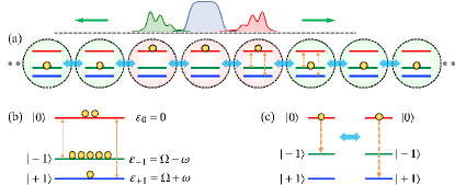
Figure 1: (a) Schematics of a periodic chain consisting of $N$ interacting three-level systems. (b) Energy levels for the onsite Hamiltonian $\hat{H}_{n}$, which depend on $\omega$ and $\Omega$ (in this demonstration $\Omega<\omega<0$, $\varepsilon_{+}<\varepsilon_{-1}<\varepsilon_{0}$). (c) A demonstration for the interaction transition between two sites, where the total magnetization is conserved, but not the onsite energy.

Interacting three-level systems - To illustrate our general idea, we consider the diffusion process in a many body system consisting of an array of $N$ three-level systems with the periodic boundary condition, and they exchange energy with the nearest neighbors (Fig. 1). Each three-level system can be regarded as a pseudo-spin (spin-1), and the full $N$-body system is described by $\hat{\mathcal{H}}=\sum_{n=1}^{N}\hat{H}_{n}+\hat{H}_{\mathrm{int}}$, where

$$\hat{H}_{n} =\Omega\,(\hat{S}_{n}^{z})^{2}+\omega\,\hat{S}_{n}^{z}=\sum_{a=0,\pm 1}\,\varepsilon_{n,a}\,|a\rangle_{n}\langle a|,$$

$$\hat{H}_{\mathrm{int}} =\sum_{n}J\,(\hat{S}_{n}^{+}\hat{S}_{n+1}^{-}+\hat{S}_{n}^{-}\hat{S}_{n+1}^{+})$$ (2)

are the onsite and interaction Hamiltonians respectively. Here $\hat{S}_{n}^{z}$, $\hat{S}_{n}^{\pm}\equiv\hat{S}_{n}^{x}\pm i\hat{S}_{n}^{y}$ are spin-1 operators on site-$n$, with $|\pm 1\rangle_{n}$ and $|0\rangle_{n}$ the eigenstates of $\hat{S}_{n}^{z}$. The onsite energy levels of site-$n$ are $\varepsilon_{n,0}=0$ and $\varepsilon_{n,\pm 1}=\Omega\pm\omega$. Except for few specific parameter sets, generally this model is nonintegrable [53].

It is easy to see that the total magnetization $\hat{\mathbf{S}}_{z}\equiv\sum_{n}\,\hat{S}_{n}^{z}$ is conserved ($[\hat{\mathbf{S}}_{z},\,\hat{\mathcal{H}}]=0$), thus the full Hilbert space can be divided into subspaces labeled by different magnon numbers. For instance, setting the fully polarized state $|\Theta\rangle:=\bigotimes_{n}|-1\rangle_{n}$ as the reference one, the 1-magnon state $|\phi_{\alpha}\rangle:=\frac{1}{\sqrt{2}}\hat{S}_{\alpha}^{+}\,|\Theta\rangle$ indicates a local excitation generated at site-$\alpha$, and all the $N$ states $\{|\phi_{\alpha}\rangle\}$ have the same total magnetization $\mathsf{S}_{z}=1-N$, which span the 1-magnon subspace. Similarly, $|\phi_{\alpha,\beta}\rangle\sim\hat{S}_{\alpha}^{+}\hat{S}_{\beta}^{+}\,|\Theta\rangle$ and $|\phi_{\alpha,\beta,\gamma}\rangle\sim\hat{S}_{\alpha}^{+}\hat{S}_{\beta}^{+}\hat{S}_{\gamma}^{+}\,|\Theta\rangle$ represent local magnon states generated on two or three local sites, and they span the 2-magnon and 3-magnon subspaces with $\mathsf{S}_{z}=2-N$ and $\mathsf{S}_{z}=3-N$ respectively. The subspace of n magnons also can be built in the same way [54, 55, 56].

Though the full Hamiltonian (2) of $3^{N}$ dimension is complicated to be solved, efficient numerical simulations of the magnon dynamics can be achieved inside the n-magnon subspace for a small n (see Appendix A). For example, the dimension for the 3-magnon subspace is $\frac{1}{6}N(N-1)(N+4)$ [54, 55, 56]. If the initial state of the system is chosen in the $n$-magnon subspace, the evolution process is well constrained within this subspace, and the full system state at any time can be obtained exactly.

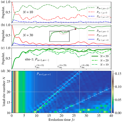
Figure 2: (a, b) The time evolution of the populations on site-1 $P_{n=1,\,a=0,\pm 1}(t)$ for chain sizes $N=10,\,30$. The dashed horizontal lines in (b) are obtained by the long time average of $P_{n=1,a}(t)$ so as to estimate their steady values in the fluctuating region. (c) The comparison of $P_{n=1,a=-1}$ for $N=10,\,20,\,30$. (d) The comparison of $P_{n=1,a=+1}$ for $N=10,11,\dots,30$. The model parameters are set as $J=0.3$, $\Omega=-1$, $\omega=-0.13$, which makes $|+1\rangle_{n}$ as the onsite ground state with $\varepsilon_{+1}<\varepsilon_{-1}<\varepsilon_{0}$ (here $|\Omega|\equiv 1$ is set as the energy unit, and the evolution time is measured by $Jt$). The recurrence times are $\tau_{\mathrm{rec}}^{(N=10)}=\tau_{\mathrm{rec}}^{(N=20)}/2=\tau_{\mathrm{rec}}^{(N=30)}/3\simeq 9.086\,J^{-1}$, which are estimated from the propagation group velocity $\tau_{\mathrm{rec}}^{(N)}:=N/v_{\mathrm{g}}$.

Diffusion of local patterns - We assume initially the system is prepared in a localized 3-magnon state $|\Psi_{0}\rangle\sim\hat{S}_{1}^{+}\hat{S}_{2}^{+}\hat{S}_{3}^{+}|\Theta\rangle$ [Fig. 1(a)], and study the time dependent diffusion process in this $N$-body system. The dynamics of the populations $P_{n=1,a}(t)$ on site-1 is shown in Fig. 2 and compared for different chain sizes $N$. At first sight, the relaxation process hardly exhibits any apparent regularity, except some seemingly “random” fluctuations. But when these evolution behaviors for difference chain sizes $N$ are compared together [Fig. 2(c, d)], we observe that their early-stage dynamics are almost identical to each other before a certain recurrence time $\tau_{\mathrm{rec}}^{(N)}$ [see the vertically parallel pattern to the left of the dashed white slope in Fig. 2(d)].

Based on the above features of the onsite population dynamics [Fig. 2(a-c)], we can generally divide the relaxation process into three stages:

1. Relaxation region ($t<\tau_{\mathrm{rec}}^{(N)}$): the onsite populations seem relaxing towards certain steady values [37], accompanied with some fluctuations;

2. Recurrence region ($t\sim\tau_{\mathrm{rec}}^{(N)}$): a recurrence “bump” appears around a recurrence time $\tau_{\mathrm{rec}}^{(N)}$ [see the inset in Fig. 2(b)], which is proportional to the chain size $N$;

3. Fluctuation region ($t>\tau_{\mathrm{rec}}^{(N)}$): the onsite populations fluctuate around certain central values, similar to a homogenous stochastic process. In addition, hierarchy recurrences appear around $t\sim\mathtt{q}\cdot\tau_{\mathrm{rec}}^{(N)}$ with $\mathtt{q}=1,2,\dots$ [the dashed white slopes in Fig. 2(d)].

Such relaxation and recurrence behaviors can be explained by the propagation of the local excitations as follows [see Fig. 1(a) and Fig. 3(a, c)] [38, 39, 40]:

Starting from the initial local excitations at site-1,2,3, the onsite population patterns $P_{n,a}(t)$ propagate and diffuse to the two sides of the chain. In the regime $t<\tau_{\mathrm{rec}}^{(N)}/2$, the patterns diffuse with a constant speed, i.e., the Lieb-Robinson group velocity [57]. Because of the finite chain size $N$, the two propagating patterns would meet each other at the other side of the periodic chain around the site $n\sim N/2$, and then propagate back to the initial starting sites, where they are superposed together. This is just the moment when a recurrence bump appears in the relaxation process of $P_{n=1,a}(t)$ [in Fig. 2(b)]. Such diffusion of the propagating patterns continues and gets superposed again and again, which results in the hierarchy recurrences appearing periodically around $t\sim\mathtt{q}\cdot\tau_{\mathrm{rec}}^{(N)}$.

The above observations suggest us defining the recurrence time as $\tau_{\mathrm{rec}}^{(N)}:=N/v_{\mathrm{g}}$, where $v_{\mathrm{g}}$ is the group velocity of the propagating patterns in the diffusion process. Here $v_{\mathrm{g}}\equiv\Delta n/\Delta t$ is numerically fitted by checking the moments that the propagating pattern of the onsite entropy $S_{n}\equiv-\mathrm{tr}[\hat{\rho}_{n}\ln\hat{\rho}_{n}]$ reaches site-$n$ [$\hat{\rho}_{n}(t)$ is the reduced density state of site-$n$], and the reaching time on site-$n$ is defined as the fastest increasing moment of $S_{n}(t)$ [e.g., see the three dots for site-5,10,15 in Fig. 3(d), corresponding to the lines in Fig. 3(c)].

The linear dependence of the recurrence time $\tau_{\mathrm{rec}}^{(N)}$ on the chain size $N$ [Fig. 2(d)] confirms that the diffusion speed $v_{\mathrm{g}}$ remains the same for different system sizes, which is consistent with the diffusion in the macroscopic world. For instance, comparing the diffusion of an ink drop in a glass of water with that in a huge pool, the diffusion speeds should be the same, but definitely it costs much longer time for the ink drop to fully diffuse all over the bigger volume.

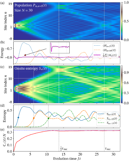
Figure 3: (a) The diffusion pattern of onsite populations $P_{n,a=0}(t)$. (b) The evolution of the average onsite energy $\sum\langle\hat{H}_{n}(t)\rangle/N$ comparing with the onsite energies $\langle\hat{H}_{n=5,10}(t)\rangle$. The horizontal gray line is calculated from the long time average of $\sum\langle\hat{H}_{n}(t)\rangle/N$. (c, d) The entropy dynamics $S_{n}(t)$ on each site. $S_{n=5,10,15}(t)$ in (d) corresponds to the three horizontal white lines in (c). The three dots in (d) are the fastest increasing point (numerically fitted). (e) The evolution of the total correlation entropy $\mathbb{C}_{\text{{t}}}(t)$, comparing with the theoretical maximum (the horizontal dashed blue line). The chain size is chosen as $N=30$, and all the other parameters are the same as in Fig. 2.

Dynamical irreversibility - The above dynamical behaviors of the pattern propagations well exhibit how the macroscopic diffusion behavior emerge with the increase of the system size $N$. In the thermodynamic limit $N\rightarrow\infty$, within a finite observation time $(t\ll\tau_{\mathrm{rec}}\sim\infty$), we would be convinced that the system is relaxing towards a certain steady state irreversibly. But here we still need a physical quantity to describe such dynamical irreversibility, which corresponds to the entropy increase in the standard macroscopic thermodynamics.

For such a time-dependent nonequilibrium process, the temperature is not well defined, thus the concept of thermal entropy $\text{\dj}Q/T$ does not apply either. Since the full system follows the unitary evolution, the von Neumann entropy of the full $N$-body state $\hat{\boldsymbol{\rho}}(t)$ always keeps a constant as the initial one [4, 3, 1, 2]. On the other hand, the onsite entropy of each individual site fluctuates from time to time [Fig. 3(c, d)], thus cannot be used as the indicator for the above irreversibility in this nonequilibrium process either.

Instead, we suggest using the total correlation entropy to describe the aforementioned dynamical irreversibility, which is defined as [42, 43, 44, 45]

$$\mathbb{C}_{\text{{t}}}[\hat{\boldsymbol{\rho}}]:=\sum_{n=1}^{N}S_{\text{{v}}}[\hat{\rho}_{n}]-S_{\text{{v}}}[\hat{\boldsymbol{\rho}}].$$ (3)

Here $S_{\text{{v}}}[\hat{\rho}]\equiv-\mathrm{tr}[\hat{\rho}\ln\hat{\rho}]$ is the von Neumann entropy, and $\hat{\rho}_{n}$ are the reduced one-body states of the full $N$-body state $\hat{\boldsymbol{\rho}}$. $\mathbb{C}_{\text{{t}}}[\hat{\boldsymbol{\rho}}]$ measures the total amount of correlations inside the $N$-body system [42, 44]. For two body systems ($N=2)$, $\mathbb{C}_{\text{{t}}}[\hat{\boldsymbol{\rho}}]$ is reduced to the mutual information, which is widely used as a measure for the bipartite correlation.

It turns out that the total correlation entropy $\mathbb{C}_{\text{{t}}}[\hat{\boldsymbol{\rho}}(t)]$ roughly exhibits a monotonically increasing behavior during the diffusion process [Fig. 3(e)]. Around the time $t\sim\tau_{\mathrm{rec}}/2$, the total correlation reaches its maximum, and hereafter almost keeps this maximal value, accompanied by only quite small fluctuations. Such behaviors are well consistent with the irreversible entropy increase in the standard macroscopic thermodynamics.

Based on such an increasing behavior, now we ask: what is the possible maximum of the total correlation after a long time growth? To find out this theoretical maximum, we consider the variation of $\mathbb{C}_{\text{{t}}}[\{p_{n,a}\}]=-\sum_{n,a}\,p_{n,a}\ln p_{n,a}$ over all possible population configurations $\{p_{n,a}\}$ for each onsite levels. Here some constraint conditions should be taken into account: (1) probability normalization $p_{n,+1}+p_{n,0}+p_{n,+1}=1$, (2) total magnetization conservation $\sum_{n}\,(p_{n,+1}-p_{n,-1})=\mathsf{S}_{z}$. In addition, though not exactly conserved, it is reasonable to assume the total onsite energy $\sum_{n}\,\langle\hat{H}_{n}(t)\rangle$ would approximately remain the same as the initial one, especially when the interaction strength $J$ is small [see Fig. 3(b)], and that gives another constraint (3) $\sum_{n,a}\,\varepsilon_{n,a}\,p_{n,a}\simeq\mathcal{E}_{0}$.

With the help of Lagrangian multipliers [58, 59], it can be proved that the theoretical maximum of the total correlation is achieved when each individual site takes the state (see Appendix B)

$$\tilde{\varrho}_{n}\sim\exp(-\beta_{\text{{e}}}\,\hat{H}_{n}-\beta_{\text{{s}}}\,\hat{S}_{n}^{z}),$$ (4)

where $\beta_{\text{{e,s}}}$ are two Lagrangian multipliers shared by all the $N$ sites, and they can be determined from the above constraints and the initial state. Clearly this state has a form of a generalized Boltzmann distribution [60, 61], thus we call it a generalized one-body Boltzmann state (GOBBS).

For the example of the parameters in Fig. 2, the total onsite energy from the initial state gives $\mathcal{E}_{0}=(N-3)\varepsilon_{-1}$ with $N=30$, and it turns out the above theoretical maximum from variation is achieved when all the sites take the same distribution $\tilde{p}_{n,-1}=0.9$, $\tilde{p}_{n,0}=0.1$, $\tilde{p}_{n,+1}=0$, which gives the possible maximum $\tilde{\mathbb{C}}_{\text{{t}}}/N\simeq 0.3251$ [dashed blue line in Fig. 3(e)]. It is worth noting that in this example the three energy levels satisfy $\varepsilon_{+1}<\varepsilon_{-1}<\varepsilon_{0}$, showing that such a distribution clearly does not obey the standard Boltzmann one that solely depends on the energies exponentially.

Now we compare this theoretical maximum with the numerical results obtained from the exact time evolution. The total onsite energy does remain similar to the initial value [purple line in Fig. 3(b)], and shows much weaker fluctuation than each individual sites, which guarantees the constraint (3) is reliable enough. In the fluctuation region ($t>\tau_{\mathrm{rec}}$), the local observable expectations (e.g., the onsite populations, energy) fluctuate around certain central values, which can be regarded as the “steady” states of the relaxation process. Thus, long time averages could eliminate these fluctuations and give a reasonable estimation for these steady values (see Appendix D). In this sense, under the parameters in Fig. 2, the steady values of onsite populations are obtained as $p_{n,-1}^{\infty}\simeq 0.9069$, $p_{n,0}^{\infty}\simeq 0.0862$, $p_{n,+1}^{\infty}\simeq 0.0069$ [dashed horizontal lines in Fig. 2(b)], which give the steady total correlation as $\mathbb{C}_{\text{{t}}}^{\infty}/N\simeq 0.3342$, and this turn out to be highly coincident with the theoretical maximum $\tilde{\mathbb{C}}_{\text{{t}}}/N\simeq 0.3251$ [dashed blue line in Fig. 3(e)].

Summary - In this paper, we study the relaxation dynamics in an isolated many body system. Though the whole system experience the reversible unitary evolution, the dynamics of the local states exhibit irreversible relaxation behaviors; the entropy of the full many body state keeps unchanged, while the total correlation entropy exhibits a monotonically increasing behavior, which well indicates the dynamical irreversibility of the relaxation process [46, 47, 48, 49, 50, 51, 52, 39, 40]. Indeed, most macroscopic thermodynamic observables in practice only involve the multi-particle average of local observables (e.g., the gas temperature and pressure are determined by the average energy of single molecular). Therefore, based on the similar idea, here we only focus on local states and observable expectations, but do not concern whether the full $N$-body state could reach the microcanonical or Gibbs state.

More importantly, we find that the total correlation entropy approximately exhibits a monotonically increasing behavior. Moreover, the variation analysis shows that, the theoretical correlation maximum would be achieved when each individual site stays in a GOBBS which is no longer solely determined by energies, and surprisingly this theoretical maximum is highly coincident with the the exact time dependent evolution. Namely, the local sites appear approaching GOBBS as their steady states irreversibly. In this sense, the entropy of the full state keeps unchanged, while the total correlation entropy exhibit the irreversible growth, which serves as a potential generalization for the irreversible entropy production in the standard thermodynamics.

Acknowledgments - SWL appreciates quite much for the helpful discussion with Z. H. Wang and L.-P. Yang. NW is supported by the National Key Research and Development Program of China under Grant No. 2021YFA1400803.

Appendix A Matrix elements of the Hamiltonian in the 3-magnon subspace

Here we write down the matrix elements of the system Hamiltonian in the local magnon basis. Since the magnon number is conserved in this system, to obtain the eigenstates of the $N$-body Hamiltonian, the diagonalization process can be constrained in the $n$-magnon subspace.

Focusing on the 3-magnon subspace spanned by $|\phi_{\alpha,\beta,\gamma}\rangle\sim\hat{S}_{\alpha}^{+}\hat{S}_{\beta}^{+}\hat{S}_{\gamma}^{+}\,|\Theta\rangle$ with $|\Theta\rangle:=\bigotimes_{n}|-1\rangle_{n}$, the matrix elements of the system Hamiltonian are given by $\langle\phi_{\alpha^{\prime}\beta^{\prime}\gamma^{\prime}}|\hat{\mathcal{H}}|\phi_{\alpha\beta\gamma}\rangle$. Since different permutation orders of $\alpha,\beta,\gamma$ are equivalent, when arranged in the ascending order $\alpha\leq\beta\leq\gamma$, the basis states $|\phi_{\alpha\beta\gamma}\rangle$ can be divided into two types ($\alpha,\beta,\gamma$ cannot be equal to each other at the same time):

1. $1\leq\alpha<\beta<\gamma\leq N$, totally $C_{N}^{3}$ states;

2. $1\leq\alpha=\beta<\gamma\leq N$ and $1\leq\alpha<\beta=\gamma\leq N$, totally $2C_{N}^{2}$ states.

Thus the dimension of the 3-magnon subspace is $\frac{1}{6}N(N-1)(N+4)$.

Now we write down the matrix elements of the operators under the basis $|\phi_{\alpha\beta\gamma}\rangle$. For $\hat{S}_{n}^{z}$, notice that $\langle\phi_{\alpha^{\prime}\beta^{\prime}\gamma^{\prime}}|\hat{S}_{n}^{z}|\phi_{\alpha\beta\gamma}\rangle=\delta_{\alpha\alpha^{\prime}}\delta_{\beta\beta^{\prime}}\delta_{\gamma\gamma^{\prime}}\,\langle\phi_{\alpha\beta\gamma}|\hat{S}_{n}^{z}|\phi_{\alpha\beta\gamma}\rangle$ is diagonal, and these matrix elements can be summarized as (here the order in the indices is irrelevant)

$$\begin{cases}\langle\phi_{\alpha,\beta,\gamma}|\hat{S}_{n}^{z}|\phi_{\alpha,\beta,\gamma}\rangle=-1,&n\neq\alpha,\beta,\gamma\\ \langle\phi_{n,\beta,\gamma}|\hat{S}_{n}^{z}|\phi_{n,\beta,\gamma}\rangle=0,&n\neq\beta,\gamma\ \text{and }\beta\neq\gamma\\ \langle\phi_{n,n,\gamma}|\hat{S}_{n}^{z}|\phi_{n,n,\gamma}\rangle=1,&n\neq\gamma\end{cases}$$ (5)

In the first line, $\alpha,\beta,\gamma$ are not necessarily to be equal or unequal to each other.

For the interaction terms $\langle\phi_{\alpha^{\prime}\beta^{\prime}\gamma^{\prime}}|\hat{S}_{n}^{+}\hat{S}_{n+1}^{-}|\phi_{\alpha\beta\gamma}\rangle$, the nonzero elements require that $\hat{S}_{n}^{+}\hat{S}_{n+1}^{-}|\phi_{\alpha\beta\gamma}\rangle$ must be still in the 3-magnon subspace, thus at least one of $\alpha,\beta,\gamma$ must be $n+1$, otherwise $\hat{S}_{n+1}^{-}|\phi_{\alpha\beta\gamma}\rangle=0$. As a result, the nonzero elements of $\langle\phi_{\alpha^{\prime}\beta^{\prime}\gamma^{\prime}}|\hat{S}_{n}^{+}\hat{S}_{n+1}^{-}|\phi_{\alpha\beta\gamma}\rangle$ can be summarized as (here the order in the indices is irrelevant)

$$\langle\phi_{n,\beta,\gamma}|\hat{S}_{n}^{+}\hat{S}_{n+1}^{-}|\phi_{n+1,\beta,\gamma}\rangle=2,$$ (6)

where $\beta,\gamma\in\{1,\dots,N\}$ , but cannot take $n+1$ or $n$ at the same time.

Similarly, when considering the long range interaction, the nonzero elements of $\hat{S}_{n}^{+}\hat{S}_{n+d}^{-}$ are $\langle\phi_{n,\beta,\gamma}|\hat{S}_{n}^{+}\hat{S}_{n+d}^{-}|\phi_{n+d,\beta,\gamma}\rangle=2$, where $\beta,\gamma\in\{1,\dots,N\}$, but cannot take $n+d$ or $n$ at the same time.

Appendix B Correlation maximization

Here we show how the theoretical maximum of the total correlation is obtained with the help of the Lagrangian multipliers. During the evolution, the density state of each individual site keeps diagonal, $\hat{\varrho}_{n}(t)=\sum_{a}\,p_{n,a}(t)\,|a\rangle_{n}\langle a|$, and we need to consider three constraint conditions: (1) probability normalization $p_{n,+1}+p_{n,0}+p_{n,+1}=1$, (2) total magnetization conservation $\sum_{n}\,(p_{n,+1}-p_{n,-1})=\mathsf{S}_{z}$, (3) the approximate conservation of total onsite energy $\sum_{n,a}\,\varepsilon_{n,a}p_{n,a}\simeq\mathcal{E}_{0}$. Thus, to find out the possible maximum of the total correlation entropy among all possible population configurations $\{p_{n,a}\}$, we study the variation on the following quantity,

$$\mathcal{T}:= -\sum_{n,a}p_{n,a}\ln p_{n,a}-\beta_{\text{{s}}}\Big{[}\mathsf{S}_{z}-\sum_{n}(p_{n,+1}-p_{n,-1})\Big{]}$$

$$- \beta_{\text{{e}}}\Big{[}\mathcal{E}_{0}-\sum_{n,a}\varepsilon_{n,a}\,p_{n,a}\Big{]}-\sum_{n}\lambda_{n}(1-\sum_{a}p_{n,a}).$$ (7)

Here $\beta_{\text{{e,s}}}$, $\lambda_{n}$ are Lagrangian multipliers, and the variation gives

$$\frac{\partial\mathcal{T}}{\partial p_{n,+1}} =-\ln p_{n,+1}-1+\beta_{\text{{s}}}+\beta_{\text{{e}}}\varepsilon_{n,+1}+\lambda_{n}\equiv 0,$$

$$\frac{\partial\mathcal{T}}{\partial p_{n,-1}} =-\ln p_{n,-1}-1-\beta_{\text{{s}}}+\beta_{\text{{e}}}\varepsilon_{n,-1}+\lambda_{n}\equiv 0,$$

$$\frac{\partial\mathcal{T}}{\partial p_{n,0}} =-\ln p_{n,0}-1+\lambda_{2}\varepsilon_{n,0}+\lambda_{n}\equiv 0.$$ (8)

These three equations further gives

$$\ln(p_{n,+1}/p_{n,0}) =\beta_{\text{{e}}}(\varepsilon_{n,+1}-\varepsilon_{n,0})+\beta_{\text{{s}}},$$

$$\ln(p_{n,-1}/p_{n,0}) =\beta_{\text{{e}}}(\varepsilon_{n,-1}-\varepsilon_{n,0})-\beta_{\text{{s}}}.$$ (9)

The solution of these two equations can be written as

$$\tilde{\varrho}_{n}\sim\exp(-\beta_{\text{{e}}}\,\hat{H}_{n}-\beta_{\text{{s}}}\,\hat{S}_{n}^{z}).$$ (10)

Namely, the possible maximum of the total correlation entropy is achieved if the reduced density matrix of each site take $\tilde{\varrho}_{n}$. Clearly, such a state has a form of a generalized one-body Boltzmann distribution, and all the $N$ sites share the same two parameters $\beta_{\text{{e,s}}}$, which can be further determined from the above constraints.

For the example of the homogeneous case, since all $\hat{H}_{n}$ have the same form, all the $N$ sites have the same distribution, i.e., $p_{n,a}\equiv\tilde{p}_{a}$, and the above constraints give

$$\tilde{p}_{+1}-\tilde{p}_{-1}=\mathsf{S}_{z}/N,$$

$$\varepsilon_{+1}\,\tilde{p}_{+1}+\varepsilon_{0}\,\tilde{p}_{0}+\varepsilon_{-1}\,\tilde{p}_{-1}=\mathcal{E}_{0}/N,$$ (11)

$$\tilde{p}_{+1}+\tilde{p}_{0}+\tilde{p}_{-1}=1,$$

which gives the result shown in the main text.

Appendix C Connection with the Boltzmann gas in the standard thermodynamics

For an isolated classical gas with weak collisions, the full ensemble state $\boldsymbol{\rho}(\vec{P},\vec{Q},t)$ of the $N$-body system follows the Liouville equation $\partial_{t}\boldsymbol{\rho}=-\{\,\boldsymbol{\rho},\,\mathcal{H}(\vec{P},\vec{Q})\,\}$ [here $(\vec{P},\vec{Q}):=(\vec{p}_{1},\vec{p}_{2},\dots;\vec{q}_{1},\vec{q}_{2},\dots)$]. As a result, the Gibbs entropy of the full $N$-body state,

$$S_{\text{{g}}}[\boldsymbol{\rho}(\vec{P},\vec{Q},t)]=-\int d^{3N}p\,d^{3N}q\,\boldsymbol{\rho}\ln\boldsymbol{\rho},$$ (12)

never changes with time.

On the other hand, if we focus on the one-particle probability distribution function (PDF) $\varrho(\mathbf{p}_{1},\mathbf{r}_{1},t)$, it can be described by Boltzmann’s transport equation (denoting $\mathrm{d}\boldsymbol{\varsigma}_{i}:=d^{3}\mathbf{r}_{i}\,d^{3}\mathbf{p}_{i}$) [52],

$$\big{[}\partial_{t}+ \frac{\mathbf{p}_{1}}{m}\cdot\nabla_{\mathbf{r}_{1}}\big{]}\,\varrho(\mathbf{p}_{1},\mathbf{r}_{1},t)$$

$$= \int(\rho_{1^{\prime}2^{\prime}}-\rho_{12})\chi_{[12\rightarrow 1^{\prime}2^{\prime}]}\,\mathrm{d}\boldsymbol{\varsigma}_{1}^{\prime}\,\mathrm{d}\boldsymbol{\varsigma}_{2}^{\prime}\,\mathrm{d}\boldsymbol{\varsigma}_{2}.$$ (13)

The LHS roots from the free motion of the single particle, while the RHS comes from the two-body collision with the other particles. Here $\chi_{[12\rightarrow 1^{\prime}2^{\prime}]}$ denotes the transition ratio from the initial state $(\mathbf{p}_{1}\mathbf{r}_{1};\,\mathbf{p}_{2}\mathbf{r}_{2})$ scattered into the final state $(\mathbf{p}_{1}^{\prime}\mathbf{r}_{1}^{\prime};\,\mathbf{p}_{2}^{\prime}\mathbf{r}_{2}^{\prime})$, and $\rho_{12}\equiv\rho(\mathbf{p}_{1}\mathbf{r}_{1};\,\mathbf{p}_{2}\mathbf{r}_{2},t)$, $\rho_{1^{\prime}2^{\prime}}\equiv\rho(\mathbf{p}_{1}^{\prime}\mathbf{r}_{1}^{\prime};\,\mathbf{p}_{2}^{\prime}\mathbf{r}_{2}^{\prime},t)$ indicate the two-particle joint PDF.

For further discussions, the molecular-disorder assumption is needed, i.e., the two-particle joint PDF approximately equals the product of the two one-particle PDF $\rho(\mathbf{p}_{1}\mathbf{r}_{1};\mathbf{p}_{2}\mathbf{r}_{2},t)\simeq\varrho(\mathbf{p}_{1},\mathbf{r}_{1},t)\cdot\varrho(\mathbf{p}_{2},\mathbf{r}_{2},t)$. That would further lead to the Boltzmann H-theorem, i.e., it turns out the entropy of the one-particle PDF,

$$S[\varrho(\mathbf{p},\mathbf{r},t)]=-\int d^{3}p\,d^{3}r\,\varrho\ln\varrho,$$ (14)

keeps increasing monotonically, until the one-particle PDF $\varrho(\mathbf{p},\mathbf{r},t)$ reaches the Boltzmann-Maxwell distribution $\varrho\sim\exp\big{[}-\beta_{\text{{e}}}\,H(\mathbf{p},\mathbf{r})\,\big{]}$, where $H(\mathbf{p},\mathbf{r})=\mathbf{p}^{2}/2m+V(\mathbf{r})$ is the single particle Hamiltonian (the instant two-body collisions are not omitted here).

In sum, the entropy of the full $N$-body state follows the Liouville dynamics and never changes, while the entropy from the one-particle PDF exhibits the irreversible growth. In principle, the full $N$-body distribution $\boldsymbol{\rho}(\vec{P},\vec{Q},t)$ would gradually become a highly correlated state. However, generally the exact form of $\boldsymbol{\rho}(\vec{P},\vec{Q},t)$ is not concerned, since in practice the one-particle PDF $\varrho(\mathbf{p},\mathbf{r},t)$ is enough to give the expectations for most macroscopic thermodynamic observables, such as the temperature, gas pressure, and some other more general few-body correlation functions.

Our study follows the similar idea as above. Clearly, here the total correlation entropy $\mathbb{C}_{\text{{t}}}(t)=\sum_{n}\,S[\varrho(\mathbf{p}_{n},\mathbf{r}_{n},t)]-S_{\text{{g}}}[\boldsymbol{\rho}(\vec{P},\vec{Q},t)]$ well returns the irreversible entropy increase behavior in the standard thermodynamics quantitatively.

Appendix D The long time behavior of local observables

In our study, we mainly focus on the time dependent evolution of the expectations for local observables, such as the populations and onsite energy of each individual site, which are calculated by

$$\langle\hat{o}(t)\rangle =\langle\Psi_{0}|\,e^{i\hat{H}t}\,\hat{o}\,e^{-i\hat{H}t}|\Psi_{0}\rangle$$

$$=\sum_{k,q}\langle E_{k}|\hat{o}|E_{q}\rangle\cdot\langle\Psi_{0}|E_{k}\rangle\langle E_{k}|\Psi_{0}\rangle\cdot e^{i(E_{k}-E_{q})t}.$$

From the numerical results shown in the main text, it can be noticed that the dynamics of these local observable expectations generally contains three stages: (1) relaxation region ($t\apprle\tau_{\mathrm{rec}}$), (2) recurrence region ($t\sim\tau_{\mathrm{rec}}$), (3) fluctuation region ($t\apprge\tau_{\mathrm{rec}}$).

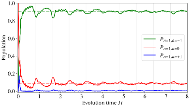
Figure 4: The time dependent evolution of the populations on site-1 $P_{n=1,\,a=0,\pm 1}$. Here the model parameters are set as $N=30$, $J=10$, $\Omega=-1$, $\omega=-0.13$. The recurrence time is estimated from the propagation pattern of the onsite entropy as mentioned in the main text, which gives $\tau_{\mathrm{rec}}\simeq 0.8015\,J^{-1}$ (the solid vertical gray lines). The dashed horizontal lines are calculated by the time averages, i.e., $p_{n,a}^{\infty}$.

In the fluctuation region, these local observable expectations $\langle\hat{o}(t)\rangle$ exhibit some seemingly “random” and small fluctuations around certain central values. In this sense, the central values of these fluctuations can be regarded as the final destination of the relaxation process. To find out the central values of these fluctuations, the long time average makes a reasonable estimation by cancelling the fluctuations, i.e.,

$$o_{\infty}:=\lim_{T\rightarrow\infty}\frac{1}{T}\int_{0}^{T}dt\,\langle\hat{o}(t)\rangle=\sum_{k}\langle E_{k}|\hat{o}|E_{k}\rangle\left|\langle\Psi_{0}|E_{k}\rangle\right|^{2}.$$

Such a treatment of long time average also has been widely adopted in thermalization problems which were based on the idea of ergodicity. In our study, the “steady states” of the onsite populations $p_{n,a}^{\infty}$ and the long time average of the total onsite energy are calculated in this way.

Fig. 4 shows the evolution for a long time. In the fluctuation region long after the relaxation, the populations $P_{n,a}(t)$ exhibit small fluctuations around certain central values, and these fluctuation centers can be well estimated by the above time average ($p_{n=1,a=-1}^{\infty}\simeq 0.9057$, $p_{n=1,a=0}^{\infty}\simeq 0.0886$, $p_{n=1,a=-1}^{\infty}\simeq 0.0057$). Besides, clearly the appearance moments of the hierarchy recurrences well fit the relation $t\sim\mathtt{q}\cdot\tau_{\text{rec}}$ with $\mathtt{q}=1,2,\dots$ (see the solid vertical gray lines).

References

- Mackey [1989] M. C. Mackey, The dynamic origin of increasing entropy, Rev. Mod. Phys. 61, 981 (1989).
- Landi and Paternostro [2021] G. T. Landi and M. Paternostro, Irreversible entropy production: From classical to quantum, Rev. Mod. Phys. 93, 035008 (2021).
- Hobson [1966] A. Hobson, Irreversibility in Simple Systems, Am. J. Phys. 34, 411 (1966).
- Huang [1987] K. Huang, Statistical Mechanics, 2nd ed. (Wiley, New York, 1987).
- Swendsen [2008] R. H. Swendsen, Explaining irreversibility, Am. J. Phys. 76, 643 (2008).
- Boltzmann [1872] L. Boltzmann, Weitere Studien über das Wärmegleichgewicht unter Gasmolekülen, Wiener Berichte 66, 275 (1872).
- Chliamovitch et al. [2017] G. Chliamovitch, O. Malaspinas, and B. Chopard, Kinetic Theory beyond the Stosszahlansatz, Entropy 19, 381 (2017).
- Gibbs [1902] J. W. Gibbs, Elementary Principles in Statistical Mechanics (C. Scribner’s sons, 1902).
- Boltzmann [1877] L. Boltzmann, Über die beziehung dem zweiten Haubtsatze der mechanischen Wärmetheorie und der Wahrscheinlichkeitsrechnung respektive den Sätzen über das Wärmegleichgewicht, Wiener Berichte 76, 373 (1877).
- Ueda [2020] M. Ueda, Quantum equilibration, thermalization and prethermalization in ultracold atoms, Nat. Rev. Phys. 2, 669 (2020).
- Deutsch [1991] J. M. Deutsch, Quantum statistical mechanics in a closed system, Phys. Rev. A 43, 2046 (1991).
- Srednicki [1994] M. Srednicki, Chaos and quantum thermalization, Phys. Rev. E 50, 888 (1994).
- Rigol et al. [2008] M. Rigol, V. Dunjko, and M. Olshanii, Thermalization and its mechanism for generic isolated quantum systems, Nature 452, 854 (2008).
- Polkovnikov et al. [2011] A. Polkovnikov, K. Sengupta, A. Silva, and M. Vengalattore, Colloquium: Nonequilibrium dynamics of closed interacting quantum systems, Rev. Mod. Phys. 83, 863 (2011).
- D’Alessio et al. [2016] L. D’Alessio, Y. Kafri, A. Polkovnikov, and M. Rigol, From quantum chaos and eigenstate thermalization to statistical mechanics and thermodynamics, Adv. Phys. 65, 239 (2016).
- Rigol [2009] M. Rigol, Breakdown of Thermalization in Finite One-Dimensional Systems, Phys. Rev. Lett. 103, 100403 (2009).
- Buča [2023] B. Buča, Unified Theory of Local Quantum Many-Body Dynamics: Eigenoperator Thermalization Theorems, Phys. Rev. X 13, 031013 (2023).
- Rigol et al. [2007] M. Rigol, V. Dunjko, V. Yurovsky, and M. Olshanii, Relaxation in a Completely Integrable Many-Body Quantum System: An Ab Initio Study of the Dynamics of the Highly Excited States of 1D Lattice Hard-Core Bosons, Phys. Rev. Lett. 98, 050405 (2007).
- Oganesyan and Huse [2007] V. Oganesyan and D. A. Huse, Localization of interacting fermions at high temperature, Phys. Rev. B 75, 155111 (2007).
- Pal and Huse [2010] A. Pal and D. A. Huse, Many-body localization phase transition, Phys. Rev. B 82, 174411 (2010).
- Altman [2018] E. Altman, Many-body localization and quantum thermalization, Nature Physics 14, 979 (2018).
- Abanin et al. [2019] D. A. Abanin, E. Altman, I. Bloch, and M. Serbyn, Colloquium : Many-body localization, thermalization, and entanglement, Rev. Mod. Phys. 91, 021001 (2019).
- Žnidarič et al. [2008] M. Žnidarič, T. Prosen, and P. Prelovšek, Many-body localization in the Heisenberg X X Z magnet in a random field, Phys. Rev. B 77, 064426 (2008).
- Wouters et al. [2014] B. Wouters, J. De Nardis, M. Brockmann, D. Fioretto, M. Rigol, and J.-S. Caux, Quenching the Anisotropic Heisenberg Chain: Exact Solution and Generalized Gibbs Ensemble Predictions, Phys. Rev. Lett. 113, 117202 (2014).
- Pozsgay et al. [2014] B. Pozsgay, M. Mestyán, M. A. Werner, M. Kormos, G. Zaránd, and G. Takács, Correlations after Quantum Quenches in the X X Z Spin Chain: Failure of the Generalized Gibbs Ensemble, Phys. Rev. Lett. 113, 117203 (2014).
- Turner et al. [2018] C. J. Turner, A. A. Michailidis, D. A. Abanin, M. Serbyn, and Z. Papić, Weak ergodicity breaking from quantum many-body scars, Nature Physics 14, 745 (2018).
- Schecter and Iadecola [2019] M. Schecter and T. Iadecola, Weak Ergodicity Breaking and Quantum Many-Body Scars in Spin-1 X Y Magnets, Phys. Rev. Lett. 123, 147201 (2019).
- Sala et al. [2020] P. Sala, T. Rakovszky, R. Verresen, M. Knap, and F. Pollmann, Ergodicity Breaking Arising from Hilbert Space Fragmentation in Dipole-Conserving Hamiltonians, Phys. Rev. X 10, 011047 (2020).
- Serbyn et al. [2021] M. Serbyn, D. A. Abanin, and Z. Papić, Quantum many-body scars and weak breaking of ergodicity, Nature Physics 17, 675 (2021).
- Desaules et al. [2023] J.-Y. Desaules, A. Hudomal, D. Banerjee, A. Sen, Z. Papić, and J. C. Halimeh, Prominent quantum many-body scars in a truncated Schwinger model, Phys. Rev. B 107, 205112 (2023).
- Łydżba et al. [2023] P. Łydżba, M. Mierzejewski, M. Rigol, and L. Vidmar, Generalized Thermalization in Quantum-Chaotic Quadratic Hamiltonians, Phys. Rev. Lett. 131, 060401 (2023).
- Hänggi et al. [1990] P. Hänggi, P. Talkner, and M. Borkovec, Reaction-rate theory: fifty years after Kramers, Rev. Mod. Phys. 62, 251 (1990).
- Zwanzig [2001] R. Zwanzig, Nonequilibrium statistical mechanics, 1st ed. (Oxford University Press, Oxford, 2001).
- Cramer et al. [2008a] M. Cramer, A. Flesch, I. P. McCulloch, U. Schollwöck, and J. Eisert, Exploring Local Quantum Many-Body Relaxation by Atoms in Optical Superlattices, Phys. Rev. Lett. 101, 063001 (2008a).
- Cramer et al. [2008b] M. Cramer, C. M. Dawson, J. Eisert, and T. J. Osborne, Exact Relaxation in a Class of Nonequilibrium Quantum Lattice Systems, Phys. Rev. Lett. 100, 030602 (2008b).
- Flesch et al. [2008] A. Flesch, M. Cramer, I. P. McCulloch, U. Schollwöck, and J. Eisert, Probing local relaxation of cold atoms in optical superlattices, Phys. Rev. A 78, 033608 (2008).
- Calabrese and Cardy [2006] P. Calabrese and J. Cardy, Time Dependence of Correlation Functions Following a Quantum Quench, Phys. Rev. Lett. 96, 136801 (2006).
- Cardy [2014] J. Cardy, Thermalization and Revivals after a Quantum Quench in Conformal Field Theory, Phys. Rev. Lett. 112, 220401 (2014).
- Li and Sun [2021] S.-W. Li and C. P. Sun, Hierarchy recurrences in local relaxation, Phys. Rev. A 103, 042201 (2021).
- Kang and Li [2023] T. Kang and S.-W. Li, The correlational entropy production during the local relaxation in a many body system with Ising interactions, Physica A 627, 129045 (2023).
- Iglói and Rieger [2000] F. Iglói and H. Rieger, Long-Range Correlations in the Nonequilibrium Quantum Relaxation of a Spin Chain, Phys. Rev. Lett. 85, 3233 (2000).
- Watanabe [1960] S. Watanabe, Information theoretical analysis of multivariate correlation, IBM J. Res. Dev. 4, 66 (1960).
- Groisman et al. [2005] B. Groisman, S. Popescu, and A. Winter, Quantum, classical, and total amount of correlations in a quantum state, Phys. Rev. A 72, 032317 (2005).
- Zhou [2008] D. L. Zhou, Irreducible Multiparty Correlations in Quantum States without Maximal Rank, Phys. Rev. Lett. 101, 180505 (2008).
- Anza et al. [2020] F. Anza, F. Pietracaprina, and J. Goold, Logarithmic growth of local entropy and total correlations in many-body localized dynamics, Quantum 4, 250 (2020).
- Esposito et al. [2010] M. Esposito, K. Lindenberg, and C. Van den Broeck, Entropy production as correlation between system and reservoir, New J. Phys. 12, 013013 (2010).
- Ptaszyński and Esposito [2019] K. Ptaszyński and M. Esposito, Entropy Production in Open Systems: The Predominant Role of Intraenvironment Correlations, Phys. Rev. Lett. 123, 200603 (2019).
- Ptaszyński and Esposito [2023] K. Ptaszyński and M. Esposito, Quantum and Classical Contributions to Entropy Production in Fermionic and Bosonic Gaussian Systems, PRX Quantum 4, 020353 (2023).
- Manzano et al. [2016] G. Manzano, F. Galve, R. Zambrini, and J. M. R. Parrondo, Entropy production and thermodynamic power of the squeezed thermal reservoir, Phys. Rev. E 93, 052120 (2016).
- Li [2017] S.-W. Li, Production rate of the system-bath mutual information, Phys. Rev. E 96, 012139 (2017).
- You and Li [2018] Y.-N. You and S.-W. Li, Entropy dynamics of a dephasing model in a squeezed thermal bath, Phys. Rev. A 97, 012114 (2018).
- Li [2019] S.-W. Li, The Correlation Production in Thermodynamics, Entropy 21, 111 (2019).
- Mutter and Schmitt [1995] K. H. Mutter and A. Schmitt, Solvable spin-1 models in one dimension, J. Phys. A 28, 2265 (1995).
- Wu et al. [2022] N. Wu, H. Katsura, S.-W. Li, X. Cai, and X.-W. Guan, Exact solutions of few-magnon problems in the spin- S periodic XXZ chain, Phys. Rev. B 105, 064419 (2022).
- Li and Wu [2022] J. Li and N. Wu, Ground-state and dynamical properties of a spin-S Heisenberg star, Comm. Theor. Phys. 74, 085701 (2022).
- Li et al. [2024] J. Li, Y. Cao, and N. Wu, Few-magnon excitations in a frustrated spin- S ferromagnetic chain with single-ion anisotropy, Phys. Rev. B 109, 174403 (2024).
- Lieb and Robinson [1972] E. H. Lieb and D. W. Robinson, The finite group velocity of quantum spin systems, Commun. Math. Phys. 28, 251 (1972).
- Jaynes [1957] E. T. Jaynes, Information Theory and Statistical Mechanics, Phys. Rev. 106, 620 (1957).
- Jaynes [1965] E. T. Jaynes, Gibbs vs Boltzmann Entropies, Am. J. Phys. 33, 391 (1965).
- Goldstein et al. [2006] S. Goldstein, J. L. Lebowitz, R. Tumulka, and N. Zanghì, Canonical Typicality, Phys. Rev. Lett. 96, 050403 (2006).
- Popescu et al. [2006] S. Popescu, A. J. Short, and A. Winter, Entanglement and the foundations of statistical mechanics, Nature Physics 2, 754 (2006).