Extended $\delta N$ formalism

Abstract

The $\delta N$ formalism is a powerful approach to compute non-linearly the large-scale evolution of the comoving curvature perturbation $\zeta$. It assumes a set of FLRW patches that evolve independently, but in doing so, all the gradient terms are discarded, which are not negligibly small in models beyond slow-roll. In this paper, we extend the formalism to capture these gradient corrections by encoding them in a homogeneous-spatial-curvature contribution assigned to each FLRW patch. For a concrete example, we apply this formalism to the ultra-slow-roll inflation, and find that it can correctly describe the large-scale evolution of the comoving curvature perturbation from the horizon exit. We also briefly discuss non-Gaussianities in this context.

Introduction.—The curvature perturbation on comoving slices, $\zeta$, is the seed of cosmic microwave background anisotropies and large-scale structures, which are seeded by the quantum fluctuations of the inflaton field stretched out of the Hubble horizon during inflation. On super-horizon scales, the evolution of the curvature perturbation can be well described by the $\delta N$ formalism Lifshitz:1960 ; Starobinsky:1982ee ; Salopek:1990jq ; Comer:1994np ; Sasaki:1995aw ; Sasaki:1998ug ; Wands:2000dp ; Lyth:2003im ; Rigopoulos:2003ak ; Lyth:2004gb ; Lyth:2005fi , which is based on the fact that the distant Hubble patches evolve independently, i.e., according to the separate-universe approach. In this picture, quantum fluctuations exiting the Hubble horizon are described as a classical field, homogeneous on each patch but with possibly different values on each causally disconnected Hubble patch. These patches evolve independently on super-horizon scales until the end of inflation and the local expansion of each patch is described by the $e$-folding number $N$. The usual $\delta N$ formalism tells us that the curvature perturbation $\zeta$ on the final comoving hypersurface of a Hubble patch is given by the difference between its local expansion and the fiducial one, i.e., $\zeta=\delta N$, when the $e$-folding number is counted from the initial flat hypersurface. This simple formula is very useful in various inflation models, such as ultra-slow-roll inflation Namjoo:2012aa ; Chen:2013eea ; Cai:2018dkf ; Pattison:2018bct ; Pi:2022ysn , constant-roll inflation Atal:2018neu ; Atal:2019cdz ; Escriva:2023uko ; Wang:2024xdl or the curvaton scenario Sasaki:2006kq ; Fujita:2014iaa ; Ando:2017veq ; Pi:2021dft ; Chen:2023lou . Also, it can be applied to the stochastic approach Fujita:2013cna ; Fujita:2014tja ; Vennin:2015hra ; Pattison:2019hef ; Pattison:2021oen ; Briaud:2023eae .

Recently, it was shown that the separate-universe approach, as well as the $\delta N$ formalism based on it, transiently breaks down around the slow-roll-to-ultra-slow-roll transition Leach:2001zf ; Naruko:2012fe ; Domenech:2023dxx ; Jackson:2023obv . This is mainly because of the non-negligible superhorizon evolution of $\zeta$, which at the leading order is dominated by the spatial-gradient term and gives the behavior of the power spectrum $\mathcal{P}_{\zeta}\propto k^{4}$ Leach:2001zf ; Byrnes:2018txb ; Cole:2022xqc . One way of solving this problem is to wait and apply the $\delta N$ formalism only at a later time $t_{j}$ when the super-horizon evolution is again negligible. The price we have to pay is to solve the linear perturbation equation without neglecting spatial gradient up to this moment $t_{j}$, which can be more than a few $e$-folds later than the horizon-exit time $t_{k}$, and the convenience of $\delta N$ formalism is significantly lost.

In this paper, we propose a novel improvement to the separate-universe approach and an extended $\delta N$ formalism by taking into account the local spatial scalar curvature. This is another direction than the anisotropic extensions given in Ref. Abolhasani:2013zya ; Talebian-Ashkezari:2016llx ; Talebian-Ashkezari:2018cax ; Tanaka:2021dww ; Tanaka:2023gul . In this new framework, the separate universe approximates each Hubble patch as a local homogeneous and isotropic Friedmann-Lemaître-Robertson-Walker (FLRW) universe with a curvature term, which still has no causal connection with the adjacent patches. We will show that this extended $\delta N$ formalism which takes the spatial curvature of each FLRW patch into account can correctly describe the superhorizon evolution of $\zeta$: even setting the initial time at the horizon-exit moment $t_{k}$, we obtain an accurate power spectrum that fits the numerical results quite well. This implies that our extended $\delta N$ formalism can be safely applied to cases where the evolution significantly deviates from the slow-roll attractor, such as ultra-slow-roll inflation.

Extended $\delta N$ formalism.—We work with the perturbed spatial metric of the scalar-type Bardeen:1980kt ; Kodama:1984ziu ; Sasaki:1998ug

$$ds^{2}_{(3)}= \,a^{2}\left((1+2\mathcal{R})\delta_{ij}+2\frac{\partial_{i}\partial_{j}}{k^{2}}H_{T}\right)\text{d}x^{i}\text{d}x^{j},$$

where $a$ is the scale factor, and $\cal R$ is the curvature perturbation. The gauge-invariant curvature perturbation on comoving slices $\zeta$ is defined by Mukhanov:1988jd ; Sasaki:1986hm

$$\zeta:={\cal R}-\frac{aH}{\phi^{\prime}}{\delta\phi}\,,$$ (1)

where $H$ is the Hubble expansion rate, and we denote by a prime the differentiation in the conformal time, $\eta\equiv\int\text{d}t/a(t)$. $\delta\phi$ is the perturbation of the inflaton field $\phi$ in this arbitrary gauge. At linear order, $\zeta$ satisfies the following Mukhanov-Sasaki equation

$$\zeta^{\prime\prime}+2\frac{z^{\prime}}{z}\zeta^{\prime}+k^{2}\zeta=0\,,$$ (2)

with $z\equiv\phi^{\prime}/H$ and $k$ the wavenumber. Equation (2) has a trivial solution $\zeta=\text{constant}$ at the leading order of $k^{2}$, which is known as the adiabatic mode. By solving equation (2) numerically, we can get the exact result of $\zeta$ in linear-perturbation theory.

Late-time $\zeta$ can also be achieved by the $\delta N$ formalism, which is based on the superhorizon solution of (2) with $k^{2}\to 0$. However, in some models, the $k^{2}$ term may not be negligible right at the horizon exit Domenech:2023dxx ; Jackson:2023obv . Here we will first show that the $\mathcal{O}(k^{2})$ correction is important in ultra-slow-roll inflation, and then propose an extended $\delta N$ formalism to take the $k^{2}$ term into account. Equation (2) has the formal solution

$$\zeta=\zeta\left(\eta_{\rm ref}\right)u_{\rm ad}(\eta)+\zeta^{\prime}\left(\eta_{\rm ref}\right)u_{\rm nad}(\eta)\,,$$

where the adiabatic and non-adiabatic mode functions are

$$u_{\text{ad}}(\eta) =1-k^{2}\int_{\eta_{\rm ref}}^{\eta}\frac{d\eta^{\prime}}{z^{2}(\eta^{\prime})}\int_{\eta_{\rm ref}}^{\eta^{\prime}}{d\eta^{\prime\prime}}{z^{2}(\eta^{\prime\prime})}+\cdots,$$

$$u_{\text{nad}}(\eta) =z^{2}(\eta_{\rm ref})\int_{\eta_{\rm ref}}^{\eta}\frac{d\eta^{\prime}}{z^{2}(\eta^{\prime})}$$

$$\quad\times\left(1-k^{2}\int_{\eta_{\rm ref}}^{\eta^{\prime}}{d\eta^{\prime\prime}}{z^{2}(\eta^{\prime\prime})}\int_{\eta_{\rm ref}}^{\eta^{\prime\prime}}\frac{d\eta^{\prime\prime\prime}}{z^{2}(\eta^{\prime\prime\prime})}+\cdots\right).$$

Here, $\eta_{\rm ref}$ is an arbitrary reference time. When $\zeta^{\prime}(\eta_{\mathrm{ref}})\sim\mathcal{O}(k^{2})$, the mode $u_{\text{nad}}$ contributes only to $\mathcal{O}\left(k^{2}\right)$ and higher orders, and becomes important on super-horizon scales only when $z$ is rapidly decreasing as in the case of the ultra-slow-roll phase. The solutions $u_{\text{ad}}$ and $u_{\text{nad}}$ are degenerate in the sense that a part of the leading order of $u_{\text{nad}}$ can be transferred to the subleading order term in $u_{\text{ad}}$ by changing the initial time $\eta_{\rm ref}$. Furthermore, when $z$ is rapidly decreasing, the next-to-leading $k^{2}$-correction of $u_{\text{nad}}$ is in general suppressed on super-horizon scales, which does not give any growth in the later stage of inflation. On the other hand, the gradient term of the adiabatic counterpart is not always suppressed, which requires an accurate treatment even on superhorizon scales. This is our main motivation to propose the extended $\delta N$ formalism.

As a simple example, we consider the Starobinsky’s linear potential model Starobinsky:1992ts ; Ivanov:1994pa ; Biagetti:2018pjj ; Ozsoy:2019lyy ; Pi:2022zxs ., in which the potential $U\left(\phi\right)$ is piecewise linear, i.e., the potential slope $U_{\phi}$ is constant in each region given by

$${U_{\phi}}=\left\{\begin{array}[]{ll}U^{\rm I}_{\phi}\,,&(\phi<\phi_{1},\leavevmode\nobreak\ \leavevmode\nobreak\ \mbox{segment I})\,,\cr U^{\rm II}_{\phi}\,,&(\phi_{1}<\phi<\phi_{2},\leavevmode\nobreak\ \leavevmode\nobreak\ \mbox{segment II})\,,\cr U^{\rm III}_{\phi}\,,&(\phi_{2}<\phi,\leavevmode\nobreak\ \leavevmode\nobreak\ \mbox{segment III})\,,\cr\end{array}\right.$$ (3)

with $|U^{\rm I}_{\phi}|=|U^{\rm III}_{\phi}|\gg|U^{\rm II}_{\phi}|$. From now on, we use the $e$-folding number $N=\ln a$ as a time variable, with $N=0$ corresponding to the time when $a=1$. We denote the transition time of the potential slope by $N_{i}$, i.e., $\phi_{i}\equiv\phi\left(N_{i}\right)$ for $i=1,2$. The system undergoes a slow-roll evolution until $\phi=\phi_{1}$. After the transition ($\phi>\phi_{1}$), the initial large velocity at $\phi_{1}$ relative to the shallower potential slope in segment II leads to a violation of slow-roll condition for a few $e$-folds, which is called the ultra-slow-roll phase. We introduce segment III to guarantee that the contribution of $\delta N$ to $\zeta$ is mainly due to the ultra-slow-roll stage and to introduce large non-Gaussianity.

We assume that the evolution of a $k$-mode can be described by the linear-perturbation theory on sub-Hubble scales. The initial conditions for the separate-universe evolution are set at $N=N_{j}(\geq N_{k})$ by the linear-perturbation theory, and the super-horizon evolution after $N_{j}$ can be described by the $\delta N$ formalism. Of course, if we set $N_{j}$ to be the end of inflation $N_{\mathrm{end}}$, the numerical solution of the Mukhanov-Sasaki equation (2) will give the accurate linear curvature perturbation. In the standard $\delta N$ approach, for the separate universe to be accurate, one should wait until $N_{kj}\equiv N_{j}-N_{k}$ is large enough. For slow-roll inflation, a few $e$-folds can work perfectly. However, as we mentioned above, in the ultra-slow-roll inflation, for some wavenumbers which exit the horizon around the slow-roll-to-ultra-slow-roll transition, we need to set $N_{kj}$ more than a few Leach:2001zf ; Jackson:2023obv ; Domenech:2023dxx , and $\delta N$ formalism loses its convenience. However, in the extended $\delta N$ formalism that we propose below, the result is quite accurate even for $N_{kj}\approx 0$, because it takes into account the spatial curvature of the foliation in its initial condition.

For simplicity, we adopt the de Sitter approximation, which fixes the energy density to a constant, $3H_{0}^{2}$, i.e., the energy density is dominated by the constant part of the inflaton potential. For an arbitrary patch with curvature, the expansion rate is given by

$$H^{2}=H_{0}^{2}-{\cal K}e^{-2(N-N_{j})}\,,$$ (4)

where ${\cal K}$ represents the spatial curvature evaluated at the junction time $N_{j}$, and in this paper, we will neglect all terms of order $\mathcal{O}\left(\mathcal{K}^{2}\right)$ and beyond. Note that, unlike the usual Friedman equation for the entire universe, $\mathcal{K}e^{2N_{j}}$ cannot be normalized to $\pm 1$, as we do not have degrees of freedom to adjust the scale factor $a=e^{N}$ according to $\mathcal{K}$ that varies in different patches. Keeping in mind that $dN=Hdt$, the homogeneous scalar field in a spatially curved patch obeys the following Klein-Gordon equation:

$$\left[\partial_{N}^{2}+3\partial_{N}\right]\phi+\frac{{U_{\phi}}}{H_{0}^{2}}+\frac{{\cal K}}{H_{0}^{2}}e^{-2(N-N_{j})}\left(\phi_{N}+\frac{{U_{\phi}}}{H_{0}^{2}}\right)=0\,,$$ (5)

where $\phi_{N}\equiv\partial_{N}\phi$. We expand $\phi$ in powers of ${\cal K}$ as $\phi=\phi^{(0)}+\phi^{(1)}+\cdots$. At the lowest order in ${\cal K}$, we have the usual second-order differential equation, of which the solution in each segment is

$$\phi^{(0)}(N) =\phi^{(0)}(N_{*})-\frac{{U_{\phi}}}{3H_{0}^{2}}(N-N_{*})$$

$$-\frac{1}{3}\left(\phi^{(0)}_{N}(N_{*})+\frac{{U_{\phi}}}{3H_{0}^{2}}\right)\left(e^{-3(N-N_{*})}-1\right)\,,$$ (6)

for the initial conditions set at $N=N_{*}$, which refers either to $N_{j}$ or to $N_{1}$ depending on which segment is concerned and the value of $N_{k}$. It is straightforward to obtain the equation of motion for $\phi^{(1)}$ which contains the ${\cal{O}}({\cal K})$ correction,

$$\left[\partial_{N}^{2}+3\partial_{N}\right]\phi^{(1)} =-\frac{{\cal K}}{H_{0}^{2}}e^{-2(N-N_{j})}\left[\phi_{N}^{(0)}+\frac{{U_{\phi}}}{H_{0}^{2}}\right]\,,$$

and the solution at this order is

$$\phi^{(1)}(N) =\phi^{(1)}(N_{*})-\frac{1}{3}\phi^{(1)}_{N}(N_{*})\left(e^{-3\left(N-N_{*}\right)}-1\right)$$ (7)

$$+\frac{\mathcal{K}U_{\phi}}{3H_{0}^{4}}e^{-2\left(N-N_{j}\right)}\left[-\frac{2}{5}e^{-2\left(N_{*}-N\right)}+1\right.$$ (8)

$$\left.-\frac{1}{2}e^{-\left(N-N_{*}\right)}-\frac{1}{10}e^{-3\left(N-N_{*}\right)}\right]$$

$$-\frac{\mathcal{K}\phi^{(0)}_{N}(N_{*})}{6H_{0}^{2}}e^{-2\left(N-N_{j}\right)}\left[\frac{2}{5}e^{-2\left(N_{*}-N\right)}\right.$$ (9)

$$\left.-e^{-\left(N-N_{*}\right)}+\frac{3}{5}e^{-3\left(N-N_{*}\right)}\right]\,.$$ (10)

Then $\phi_{N}^{(0)}(N)$ and $\phi_{N}^{(1)}(N)$ can be calculated by taking the derivative of (6) and (7).

Knowing the evolution of the inflaton field $\phi(N)$ up to $\mathcal{O}(\mathcal{K})$, what we want to calculate is the comoving curvature perturbation $\zeta(N)$ at a late time. In the model considered in (3), as the transition from ultra-slow roll to the second slow-roll stage is abrupt, the contribution to $\delta N$ from stage III is negligible Chen:2013aj ; Cai:2018dkf ; Pi:2022ysn ; Pi:2024jwt . Therefore, the curvature perturbation will not change much after $N_{2}$ and the constant-$\phi$ hypersurface at $\phi_{2}$ is chosen as the final comoving slice, i.e., $\zeta(N_{\mathrm{end}})\approx\zeta(N_{2})$, in the analytic calculation below. The general methodology to solve the dynamics is the following.

(a) e choose the $\delta N$ gauge, in which the shift vanishes and $\mathcal{R}^{\prime}=H_{T}^{\prime}/3$ Sasaki:1998ug . In this gauge, the physical volume is proportional to $\exp\left(3N\right)$, independent of the spatial-coordinate parameterization. At $N=N_{j}$, we set the initial conditions of the field perturbation $\delta\phi$ and the curvature perturbation $\mathcal{R}$ for the $\delta N$ formalism to match the linear-perturbation theory. The results are (see the supplementary material for a proof)

$$\delta\phi\left(N_{j}\right)=0\,,\qquad\mathcal{R}\left(N_{j}\right)=\zeta\left(N_{j}\right)\,,$$ (11)

$$\delta\phi_{N}\left(N_{j}\right)=\frac{\phi_{N}}{3H_{0}^{2}}\left(-U\zeta_{N}\left(N_{j}\right)+k^{2}e^{-2N_{j}}\zeta\left(N_{j}\right)\right)\,,$$ (12)

$$\mathcal{R}_{N}\left(N_{j}\right)=\frac{\phi_{N}^{2}}{6}\zeta_{N}\left(N_{j}\right)+\frac{k^{2}}{3H_{0}^{2}}e^{-2N_{j}}\zeta\left(N_{j}\right)\,,$$ (13)

$$e^{2N_{j}}\mathcal{K}=\frac{2k^{2}}{3}\zeta\left(N_{j}\right)\,.$$ (14)

The first line comes from setting the initial surface at $N_{j}$ in the comoving slicing $\delta\phi=0$. This choice is allowed because of the existence of residual gauge freedom in the $\delta N$ gauge, which corresponds to the choice of time coordinate in each local universe Artigas:2021zdk ; Artigas:2023kyo .

In such a separate universe, the spatial gradient of the scalar field is absent in the Klein-Gordon equation of $\phi$, Eq.(5). To ensure that equation of motion for $\delta\phi$ matches with the Klein Gordon equation (5) in the perturbed universe, we set $\delta\phi=0$ at $N=N_{j}$ using the residual gauge degree of freedom. We also assume that the slow-roll suppressed first term in $\delta\phi_{N}(N_{j})$ is as small as the second term, and then $\delta\phi(N)$ remains to be $O(k^{2})$. The second and third lines in Eqs. (14) are obtained with the aid of the momentum constraint. In the last line, the effective curvature $\propto\mathcal{K}$ in the separate-universe approach is determined by the term-by-term matching of perturbed (5) and the equation of motion for $\delta\phi$ at the linear order. Equivalently, we can also get this relation by evaluating the spatial Ricci curvature on the $\delta\phi=0$ hypersurface. While the value of $k^{2}$ is necessary to give the initial condition for the long-wavelength perturbations, the long-wavelength evolution itself is completely local. In $\delta N$ gauge, the equation for $\mathcal{R}$ valid up to $O(k^{2})$ is linear and closed as

$$\frac{1}{a^{3}H_{0}}\partial_{N}\left(a^{3}H_{0}\partial_{N}{\cal R}\right)=\frac{k^{2}}{3a^{2}H_{0}^{2}}{\cal R}\,.$$ (15)

The solution under the initial conditions (14) is obtained by a perturbative expansion in $k^{2}$ as

$$\mathcal{R}(N)=\zeta\left(N_{j}\right)+\frac{k^{2}\zeta\left(N_{j}\right)}{6H_{0}^{2}}\left(e^{-2N_{j}}-e^{-2N}\right)\,.$$ (16)

The second term gives a weak time dependence, which anyway remains minor.

(b) If $N_{j}$ is in the segment I, the evolution in the segment I is given by Eqs. (6)–(7) and their derivatives, setting $N_{*}=N_{j}$. We solve the fields up to the transition at $\phi=\phi_{1}$ which provides the initial conditions for the succeeding ultra-slow-roll evolution.

(c) For the field evolution in segment II, one uses again equations (6)–(7) and their derivatives but with the initial conditions at $N_{*}\equiv N_{1}$ for $N_{j}<N_{1}$ and those at $N_{*}\equiv N_{j}$ for $N_{j}>N_{1}$.

(d) The numbers of $e$-folds in the respective segments $N_{ab}\equiv N_{b}-N_{a}$ are obtained by inverting Eqs. (6) and (7), e.g.,

$$N_{j1}= \frac{3H_{0}^{2}}{U_{\phi}^{\rm I}}\left[-\phi_{j1}+\frac{1}{3}\left(\phi_{N}(N_{j})+\frac{U_{\phi}^{\rm I}}{3H_{0}^{2}}\right)\right.$$ (17)

$$\qquad\left.-\frac{2\mathcal{K}U_{\phi}^{\rm I}}{15H_{0}^{4}}-\frac{\mathcal{K}\phi_{N}^{(0)}}{15H_{0}^{2}}\right]\,,$$ (18)

$$N_{12}= \frac{3H_{0}^{2}}{U_{\phi}^{\rm II}}\left[-\phi_{12}-\frac{1}{3}\left(\phi_{N}(N_{1})+\frac{U_{\phi}^{\rm II}}{3H_{0}^{2}}\right)\left(e^{-3N_{12}}-1\right)\right.$$ (19)

$$\qquad\left.-\frac{2\mathcal{K}U_{\phi}^{\rm II}}{15H_{0}^{4}}e^{-2N_{j1}}-\frac{\mathcal{K}\phi_{N}^{(0)}(N_{1})}{15H_{0}^{2}}e^{-2N_{j1}}\right]\,,$$ (20)

where we have neglected the remaining terms that decay exponentially fast. For a detailed comparison with the ordinary linear perturbation, see the supplementary material.

(e) The non-linear curvature perturbation on the final comoving hypersurface ($\phi=\phi_{2}$) can then be calculated as

$$\zeta\left(N_{2}\right) =\mathcal{R}\left(N_{2}\right)+\delta N_{j2}\,,$$ (21)

where $\delta N_{j2}:=N_{j2}-\bar{N}_{j2}$ with $\bar{N}_{j2}$ being the background value of $N_{j2}$. When evaluated on the $\phi=$ constant hypersurface, ${\cal R}$ is to be identified with the gauge-invariant comoving curvature perturbation. The non-linearly extension of the comoving curvature perturbation is defined by the $e$-folding number between the flat slicing and the comoving slicing.

Here, the second term on the right-hand side of Eq. (21) comes from the nonlinear gauge transformation from the time slice in the $\delta N$ gauge to the comoving slice specified by $\phi=\phi_{2}$, while the first term is the curvature perturbation at the final hypersurface in the $\delta N$ gauge. As the difference between $\mathcal{R}(N_{2})$ and $\mathcal{R}(N_{j})$ remains small, we can also approximate (21) by $\zeta(N_{2})=\mathcal{R}(N_{j})+\delta N_{j2}$, which is closer to the ordinary $\delta N$ formula.

The power spectrum of $\zeta$ can then be calculated under this formalism. When the usual separate universe is matched to perturbation theory right after the horizon exit of the $k$ mode, $N_{kj}\approx 0$, the power spectrum of $\zeta$ is incompatible between the two approaches, as shown in the upper panel in Fig  1. This discrepancy is mainly due to the $k^{2}$-correction which is neglected in the separate universe approach but is now as large as the leading order contribution. As we choose later initial hypersurfaces, i.e., larger $N_{kj}$’s, the power spectra given by the ordinary $\delta N$ formalism approach the correct result obtained by numerically solving the Mukhanov-Sasaki equation. On the other hand, in our extended $\delta N$ formalism, we take into account the spatial curvature on the initial hypersurface, which significantly alleviates the discrepancy even if we set the initial condition as early as the horizon-exit moment. This is clearly shown in the lower panel in Fig. 1. We can also see some small discrepancies from higher orders of $k^{2}$ for $N_{kj}=0$, which disappears rapidly and monotonically as we increase $N_{kj}$.

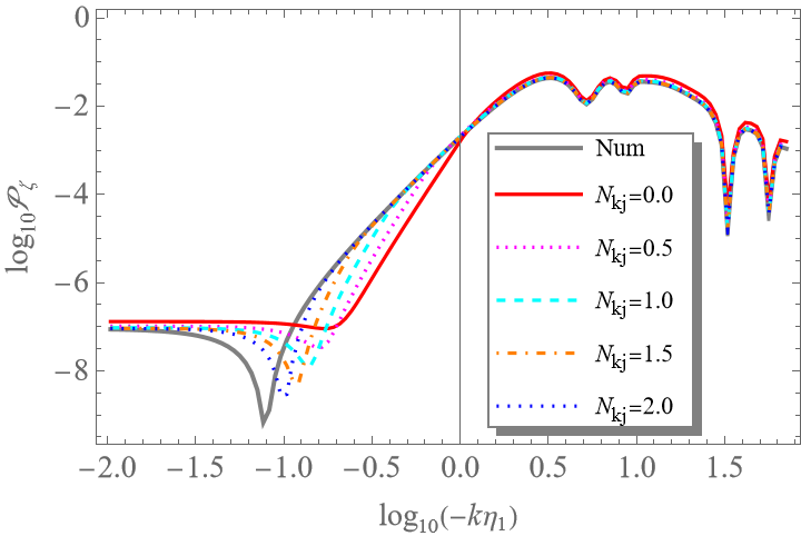
Figure 1: Power spectrum generated using the standard $\delta N$ (top) and the extended $\delta N$ formalism (bottom). Here, the parameters were fixed to $H_{0}=10^{-6}$, $U_{\phi}^{\rm I}=U_{\phi}^{\rm III}=-10^{-14}$, $U_{\phi}^{\rm II}=0$ and $\phi_{12}\approx 0.0011$ such that $N_{12}=2$. “Num” means the results obtained by solving numerically the Mukhanov-Sasaki equation until the end, and $N_{kj}=0.0$, 0.5, etc. means using different initial times in the two $\delta N$ formalisms.

Non-Gaussianities.—A non-linear treatment of these models is demanded, as non-Gaussianities of density perturbations are crucial to predict the production rate of primordial black holes Franciolini:2018vbk ; Ezquiaga:2018gbw ; Firouzjahi:2018vet ; Yoo:2019pma ; Kehagias:2019eil ; Ballesteros:2020sre ; Cai:2021zsp ; Riccardi:2021rlf ; Taoso:2021uvl ; Biagetti:2021eep ; Kitajima:2021fpq ; Pattison:2021oen ; Cai:2022erk ; Young:2022phe ; Escriva:2022pnz ; Escriva:2022duf ; Matsubara:2022nbr ; Gow:2022jfb ; LISACosmologyWorkingGroup:2023njw ; Tomberg:2023kli ; Pi:2024jwt . Here, we briefly discuss how to evaluate the non-Gaussianity parameter $f_{\rm NL}$, applying the extended $\delta N$ formalism, deferring more detailed discussion about the non-Gaussian probability distribution of the perturbation to future work.

By denoting $\zeta_{G}$ the Gaussian curvature perturbation, deviations from this Gaussianity can be captured by the quadratic term with a nonlinear parameter $f_{\rm NL}$ Komatsu:2001rj ; Maldacena:2002vr ; Bartolo:2004if ; Yokoyama:2008by ,

$$\zeta=\zeta_{G}+\frac{3}{5}f_{\rm NL}\zeta_{G}^{2}\,+\cdots.$$

Defining $\zeta_{1}=\partial\zeta(N)/\partial\zeta(N_{j})$, $\zeta_{2}=\partial\zeta(N)/\partial\zeta_{N}(N_{j})$, $\zeta_{12}=\partial^{2}\zeta(N)/\partial\zeta(N_{j})\partial\zeta_{N}(N_{j})$, etc., we can write $f_{\rm NL}$ in the following expression Yokoyama:2007dw

$$f_{\rm NL}=\frac{5}{6}\sum_{a,b,c,d,e,f=1,2}\frac{\zeta_{a}\zeta_{b}\zeta_{cd}{\cal P}^{ac}{\cal P}^{bd}}{(\zeta_{e}\zeta_{f}{\cal P}^{ef})^{2}}\,,$$ (22)

where the initial distribution of $\zeta(N_{j})$ and $\zeta_{N}(N_{j})$ is Gaussian. ${\cal P}^{ab}$ are the two-point correlation functions of $\zeta\left(N_{j}\right)$ or $\zeta_{N}\left(N_{j}\right)$ evaluated by using the standard perturbation theory of a Bunch-Davies vacuum state. Concerning the ultra-slow-roll stage, for simplicity, we set $U_{\phi}^{\rm II}=0$ for the following analytic computation. In this case, Eq. (20) simplifies to

$$N_{12}=-\frac{1}{3}\ln\beta,\leavevmode\nobreak\ \text{with}\leavevmode\nobreak\ \beta:=1-\frac{3\phi_{12}}{\phi_{N}(N_{1})}-\frac{\mathcal{K}e^{-2N_{j1}}}{5H_{0}^{2}}\,,$$

where $\phi_{N}(N_{1})$ and $N_{j1}$ are obtained from Eqs. (6)–(7), their derivatives, and Eq. (18), which depend on $\phi(N_{j})$, $\phi_{N}(N_{j})$ and ${\cal K}$. Roughly speaking, $\beta$ is approximately given by $\phi_{2v}/\phi_{1v}$ with $\phi_{v}(>\phi_{2})$ being the virtual endpoint on the flat plateau $U^{II}$, which is positive but small. Let’s assume that the contribution of $\delta N_{12}$ dominates in $\zeta(N_{2})$. Then, we expand $\beta$ between background and perturbations, respectively, as $\beta=\overline{\beta}+\delta\beta+O(\zeta(N_{j})^{2},\zeta(N_{j})\zeta_{N}(N_{j}),\zeta_{N}(N_{j})^{2})$, where $\bar{\beta}$ is the background value of $\beta$. In ultra-slow-roll inflation, the enhancement of $\delta\beta/\bar{\beta}$ is realized by the smallness of $\bar{\beta}$, hence we can neglect the higher-order terms and $\delta\beta$ is a linear function of $\zeta(N_{j})$ and $\zeta_{N}(N_{j})$, whose distributions can be well-approximated by Gaussian distributions. In this case, Eq. (22) can be reduced to

$$f_{\rm NL}=\frac{5}{6}\frac{\partial_{\bar{\beta}}^{2}N_{12}({\bar{\beta}})}{\left(\partial_{\bar{\beta}}N_{12}({\bar{\beta}})\right)^{2}}\,.$$ (23)

Then, it is easy to show that the non-linear parameter reduces to $f_{\rm NL}=5/2$. Zero or negative $\bar{\beta}$ corresponds to infinite $e$-folding number as the inflaton gets stuck on the plateau, and quantum diffusion is needed to end inflation Ezquiaga:2018gbw ; Firouzjahi:2018vet ; Ballesteros:2020sre ; Pattison:2021oen ; Tomberg:2023kli , which is beyond our scope .

Conclusion.—The $\delta N$ formalism is a non-linear approach allowing one to compute the curvature perturbation $\zeta$ by the perturbed $e$-folding number $\delta N$ in a perturbed FLRW universe. This method relies on the separate-universe approach which captures the super-horizon-scale dynamics by neglecting gradient terms of $\mathcal{O}\left(k^{2}\right)$. Effectively, it is equivalent to evolving independently a set of causally disconnected patches, each of which is a flat, homogeneous and isotropic FLRW universe. In certain scenarios, however, the adiabatic mode may exhibit important gradient corrections of ${\cal O}(k^{2})$, which leads to the breakdown of the separate-universe picture. One important example is the model with an ultra-slow-roll phase, which is among the scenarios that introduce a peak in the power spectrum. In this paper, we showed how to capture the $k^{2}$-corrections of the adiabatic mode within the framework of the $\delta N$ formalism by introducing the spatial curvature $\mathcal{K}$ in each patch of the separate universe. The initial conditions of the separate universe are identified by matching with linear-perturbation theory, and in this extended $\delta N$ formalism the curvature $\mathcal{K}$ takes care of the $k^{2}$-correction in $\zeta$. Namely, moving to the gauge in which the inflaton field takes a constant value on the equal-time hypersurface at the initial time, we absorb the spatial gradient terms into the spatial curvature of the hypersurface. By doing so, the gradient term in the Klein-Gordon equation is made irrelevant for the adiabatic mode, and one can accurately compute $\zeta$ even if the separate-universe approach is used right after the horizon exit. We illustrated this methodology in the case of a Starobinsky model and confirmed the validity of this method by explicitly comparing the resulting power spectrum of $\zeta$ with the numerical result of the linear perturbation theory. A formal proof of the validity of this method, as well as the analytic comparison with the linear-perturbation theory, is put in supplementary material. Finally, we used the extended $\delta N$ formalism to compute the non-Gaussianities of the curvature perturbation. We observed that the $f_{\rm NL}$ parameter value can make a plateau at $f_{\rm NL}=5/2$ and the plateau would contain the peak frequency of the power spectrum if the ultra-slow-roll phase abruptly transits to another slow-roll phase. From the analytic estimate, on the plateau the distribution of $\zeta$ is determined from a Gaussian distribution of $\delta{\beta}$ by the non-linear transform that takes the form of $\zeta=-\frac{1}{3}\ln\left(1+\delta\beta/\bar{\beta}\right)$. Hence, the distribution at a large positive value of $\zeta$ behaves like $\propto\exp(-3\zeta)$ Pi:2024jwt . To give the full frequency dependence of $f_{NL}$, we need more careful treatment, which we would like to defer to future work.

Acknowledgments: We thank Diego Cruces, Misao Sasaki, and David Wands for discussions and useful comments. This work is supported in part by the National Key Research and Development Program of China Grant No. 2021YFC2203004. The authors thank the YITP long-term workshop “Gravity and Cosmology 2024”, during which the basic idea of this work has been developed. D. A. is supported by JSPS Grant-in-Aid for Scientific Research No. JP23KF0247. S. P. is supported by by Project No. 12047503 of the National Natural Science Foundation of China, by JSPS KAKENHI No. JP24K00624, and by the World Premier International Research Center Initiative (WPI Initiative), MEXT, Japan. T. T. is supported by Grant-in-Aid for Scientific Research under Contract Nos. JP23H00110, JP20K03928, JP24H00963, and JP24H01809.

Appendix A Gradient expansion with local curvature

A.1 Linear perturbations

Here we focus on scalar-type perturbations. The metric of the scalar-type perturbation can be written as Bardeen:1980kt ; Kodama:1984ziu ; Sasaki:1998ug ,

$$ds^{2}=a^{2}\Big{[}-\big{(}1+2AY\big{)}d\eta^{2}-2BY_{j}d\eta dx^{j}+\big{(}(1+2H_{L})Y\delta_{ij}+2H_{T}Y_{ij}\big{)}dx^{i}dx^{j}\Big{]}.$$ (24)

where $Y$ is the spatial scalar harmonic with the eigenvalue $k^{2}$, $Y_{j}=-k^{-1}\nabla_{j}Y$, and $Y_{ij}=k^{-2}\left(\nabla_{i}\nabla_{j}Y+\frac{1}{3}\delta_{ij}\nabla^{2}Y\right)$. We associate the harmonics $Y$ explicitly to emphasize that the metric and scalar-field perturbations are to be understood as the expansion coefficients here, although we use the same notations to express the corresponding spacetime functions. The local expansion along a geodesic is

$$\tilde{N}=\int^{\eta}_{\eta_{0}}\left(\mathcal{H}+\Big{(}H_{L}^{\prime}+\frac{1}{3}kB\Big{)}Y\right)d\eta,$$ (25)

which implies the $e$-folding number $\tilde{N}$ equals to the background $N$ if we take the $\delta N$ gauge

$$H_{L}^{\prime}=B=0.$$ (26)

This gives a constraint for the curvature perturbation, $\mathcal{R}\equiv H_{L}+\frac{1}{3}H_{T}$,

$$\mathcal{R}^{\prime}=\frac{1}{3}H_{T}^{\prime}.$$ (27)

It is easy to see that there is some gauge redundancy hidden in the integration constant of (27), which we will use later to set the initial conditions of $\delta\phi$.

The $\delta N$ gauge is convenient to see the equivalence of the perturbed equation and the background equation Sasaki:1998ug . In this gauge, the perturbed Klein-Gordon equation at linear order reduces to

$$H_{0}{d\over dN}\Big{(}H{\delta\phi}_{N}\Big{)}+3H_{0}^{2}{\delta\phi}_{N}+{U_{\phi\phi}}{\delta\phi}+2{U_{\phi}}A-H_{0}^{2}{\phi_{N}}A_{N}+k^{2}e^{-2N}{\delta\phi}=0\,.$$ (28)

Thus among metric variables, the perturbed field equation contains only $A$. From the $\left({}^{0}_{0}\right)$-component of the perturbed Einstein equations, one can see that $A$ is expressed in terms of $\delta\phi$ as

$$2UA=-H_{0}^{2}\phi_{N}{\delta\phi}_{N}-{U_{\phi}}{\delta\phi}+2k^{2}e^{-2N}{\cal R}\,.$$ (29)

At this point, if one can neglect the last term proportional to $k^{2}$, one may substitute Eq. (29) into Eq. (28) to obtain a closed second-order equation for ${\delta\phi}$. From the traceless part of the $\left({}^{i}_{j}\right)$-component of Einstein equations, the equation for ${\cal R}$ can be written under the closed form

$$\frac{1}{a^{3}H_{0}}\partial_{N}\left(a^{3}H_{0}\partial_{N}{\cal R}\right)=\frac{k^{2}}{3a^{2}H_{0}^{2}}({\cal R}+A)\,.$$ (30)

Now, we recall that the $k^{2}$-correction is necessary only for the adiabatic mode. At any reference time we can set $\delta\phi=0$, attributing all the curvature perturbation $\zeta$ to ${\cal R}$, which is possible because the $\delta N$-gauge is not a complete gauge fixing (see Eq. (27)). Moreover, from the non-adiabatic mode, one can also set ${\delta\phi}_{N}=O(k^{2})$ at the reference time. Then, the above perturbation equations indicate that both $\delta\phi$ and $A$ remain $O(k^{2})$. As a result, the last term in Eq. (28) and the contribution of $A$ in Eq. (30) become $O(k^{4})$, hence providing us with a closed equation for $\mathcal{R}$.

A.2 Separate-universe mapping

In this subsection we derive the aforementioned equations for the separate universes, which are causally disconnected patches and evolve independently after $N_{j}$. Using the number of $e$-folds $N$ as the time coordinate, the Klein-Gordon equation and the FLRW equation with spatial curvature $\mathcal{K}$ defined at some initial time $N_{j}$ become

$$H{d\over dN}\left(H{\phi_{N}}\right)+3H^{2}{\phi_{N}}+{U_{\phi}}=0\,,$$ (31)

$$H^{2}\left(1-{1\over 6}\phi_{N}^{2}\right)={1\over 3}U-\mathcal{K}e^{-2\left(N-N_{j}\right)}\,.$$ (32)

From now on, we will assume that $\mathcal{K}=0$ in the unperturbed background (or equivalently, in the fiducial universe) and, therefore, $\mathcal{K}$ is thought to be first order in perturbations. For a perturbed universe, taking the variation of Eqs. (31) and (32), we obtain

$$H{d\over dN}\left(H\delta\phi_{N}\right)+3H^{2}\delta\phi_{N}+{U_{\phi\phi}}\delta\phi-2{U_{\phi}}{\delta H\over H}+H^{2}{\phi_{N}}{d\over dN}\left({\delta H\over H}\right)=0\,,$$ (33)

$$-2U{\delta H\over H}=-{H^{2}}\phi_{N}\delta\phi_{N}-{U_{\phi}}\delta\phi+3e^{-2\left(N-N_{j}\right)}\mathcal{K}\,,$$ (34)

We find these equations are, respectively, equivalent to Eqs. (28) and (29) in the $\delta N$-gauge, with the identifications

$$\frac{\delta H}{H} =-A\,,$$ (35)

$$e^{2N_{j}}\mathcal{K} =\frac{2}{3}k^{2}{\cal R}\,,$$ (36)

except for the last term on the left-hand side of Eq. (28). Equation (36) can also be obtained in the following way. Note that on a homogeneous isotropic equal-time hypersurface with a curvature term $\mathcal{K}e^{-2(N-N_{j})}$, the three-dimensional curvature is equal to $6\mathcal{K}e^{-2(N-N_{j})}$, while from the metric Eq. (24), this curvature is $-4e^{-2N}\nabla^{2}\mathcal{R}$. Then, we easily check the consistency of Eq. (36).

As mentioned above below Eq. (30), we do not need the term proportional to $k^{2}$ in Eq. (28) to obtain the adiabatic mode in an appropriate choice of the residual gauge degrees of freedom. This proves that the separate-universe description can completely reproduce the linear perturbation including the $k^{2}$-correction of the adiabatic mode, if we set the matching conditions appropriately. An important point is that the gauge-invariant comoving curvature perturbation $\zeta$ should be attributed to ${\cal R}$ as an initial condition for the separate-universe evolution. Otherwise, the last term $k^{2}e^{-2N}\delta\phi$ in Eq. (28), which is missing in Eq. (33), contributes as the correction of $O(k^{2})$.

The initial condition at $N=N_{j}$ should be provided in terms of $\zeta$ as follows:

$$\zeta(N_{j}) =\left.{\cal R}(N_{j})-\frac{\delta\phi}{\phi_{N}}\right|_{Nj}\,,$$ (37)

$$\zeta_{N}(N_{j}) =\mathcal{R}_{N}(N_{j})-\partial_{N}\left(\frac{\delta\phi}{\phi_{N}}\right)_{N_{j}}\,,$$ (38)

$$\delta\phi(N_{j}) =0\,.$$ (39)

The three equations above cannot determine four variables, ${\cal R}$, $\delta\phi$, and their derivatives. We need to supplement the condition coming from the momentum constraint, i.e., the $\left({}^{0}_{i}\right)$-component of the perturbed Einstein equations

$${\cal R}_{N}=A-{1\over 2}\phi_{N}{\delta\phi}\,.$$ (40)

Combined with Eq. (29), we eliminate $A$ to obtain another relation among the variables to be determined,

$$2U\mathcal{R}_{N}(N_{j})=-H^{2}\phi_{N}(N_{j}){\delta\phi}_{N}(N_{j})+2k^{2}e^{-2N_{j}}\mathcal{R}(N_{j})\,,$$ (41)

where we have used $\delta\phi(N_{j})=0$. Substituting (38) into (41), we can eliminate $\mathcal{R}_{N}(N_{j})$ and obtain

$$\delta\phi_{N}(N_{j})=\frac{\phi_{N}}{3H_{0}^{2}}\left(-U\zeta_{N}(N_{j})+k^{2}e^{-2N_{j}}\zeta(N_{j})\right).$$ (42)

Then substituting (42) back into (38), we can easily derive the condition for $\mathcal{R}_{N}(N_{j})$, shown in Eqs. (14).

Finally, neglecting the contribution of $A$ in Eq. (30), one can solve the equation to determine the leading $k^{2}$-correction contained in $\mathcal{R}$. If we allow to approximate $H_{0}$ to be constant, we get

$$\mathcal{R}(N) =\mathcal{R}\left(N_{j}\right)\left[1+\frac{k^{2}}{6H_{0}^{2}}e^{-2N_{j}}\left(1-e^{-2\left(N-N_{j}\right)}\right)\right]\,,$$ (43)

where we used the initial condition for $\mathcal{R}_{N}$ given in Eqs. (14), neglecting the contribution from $\zeta_{N}$ at $N=N_{j}$. After a few $e$-folds,

$$\mathcal{R}(N) \approx\left[1+\frac{k^{2}}{6H_{0}^{2}}e^{-2N_{j}}\right]\mathcal{R}\left(N_{j}\right)\,.$$ (44)

This solution clearly indicates that the $k^{2}$-correction in ${\cal R}$ remains approximately constant and does not have any enhancement factor due to the ultra-slow roll phase.

Appendix B Linear approximation in ultra-slow-roll inflation

B.1 Extended $\delta N$ for the Starobinsky model

B.1.1 Modes crossing during slow roll

For an application, we detail the calculations of the extended $\delta N$-approach in the context of linear (field) perturbations. As mentioned earlier we will assume that the background curvature vanishes such that $\mathcal{K}$ is of first-order in perturbative expansion. This means that the perturbations of the scalar field are given by

$$\delta\phi :=\delta\phi^{(0)}+\phi^{(1)}\,,$$ (45)

where we recall that in our notations, the upper index refers to the order in $\mathcal{K}$ expansion.

We start our analysis with the case where the extended $\delta N$ is matched to linear-perturbation theory during the slow-roll phase, $N_{j}<N_{1}$. From Eqs. (6) and (7), the condition $\phi_{1}\equiv\phi(N_{1})$ is explicitly written down as

$$\phi_{1} \approx\phi(N_{j})-\frac{U^{\rm I}_{\phi}}{3H_{0}^{2}}N_{j1}-\frac{1}{3}\left(\phi_{N}(N_{j})+\frac{U^{\rm I}_{\phi}}{3H_{0}^{2}}\right)\left(e^{-3N_{j1}}-1\right)-\frac{{\cal K}U^{\rm I}_{\phi}}{9H_{0}^{4}}\left(1-3e^{-2N_{j1}}\right)\,,$$ (46)

where we kept the leading order in $\mathcal{K}$, neglected the remaining terms that decay exponentially fast, and used the slow-roll condition at $N_{j}$ to rewrite $\mathcal{K}\phi^{(0)}_{N}(N_{j})=-\mathcal{K}{U_{\phi}}^{\rm I}/(3H_{0}^{2})$.

We fix the value $\phi_{1}$ at the transition such that, at linear order, $\delta\phi_{1}=0$. Expanding the above equation in perturbations, the perturbed $e$-folding number between the start and the end of the first slow-roll phase is approximated by

$$\delta N_{j1}\approx\frac{3H_{0}^{2}}{U^{\rm I}_{\phi}}\left(\delta\phi(N_{j})+\frac{1}{3}\delta\phi_{N}(N_{j})\right)-\frac{{\cal K}}{3H_{0}^{2}}\left(1-3e^{-2\bar{N}_{j1}}\right)\,,$$ (47)

where we neglect terms decaying as $e^{-3N_{j1}}$ and denote by $\bar{N}$ the background $e$-folding number (notice that $N_{j}$ is unperturbed by definition so we do not put overline to $N_{j}$ below). We focus on the adiabatic mode, whose $k^{2}$-correction is relevant. Hence, setting $\zeta^{\prime}(N_{j})=0$, the junction conditions Eqs. (14), which include $\delta\phi(N_{j})=0$, lead us to

$$\delta N_{j1}\approx-\frac{{\cal K}}{2H_{0}^{2}}+\frac{\cal K}{H_{0}^{2}}e^{-2\bar{N}_{j1}}\approx-\frac{k^{2}\zeta_{j}}{3H_{0}^{2}}e^{-2N_{j}}+\frac{2k^{2}\zeta_{j}}{3H_{0}^{2}}e^{-2\bar{N}_{1}}\,.$$ (48)

In the first equality, we neglect the term decaying like $e^{-3N_{1}}$. The comoving curvature perturbation $\zeta$ at $N_{1}$ at linear order is therefore evaluated by

$$\zeta_{j1} =\delta N_{j1}+\frac{k^{2}\zeta_{j}}{6H_{0}^{2}}\left(e^{-2N_{j}}-e^{-2\bar{N}_{1}}\right)\approx-\frac{k^{2}\zeta_{j}}{6H_{0}^{2}}e^{-2N_{j}}+\frac{k^{2}\zeta_{j}}{2H_{0}^{2}}e^{-2\bar{N}_{1}}\,,$$ (49)

with the $k^{2}$-correction also provided by linear-perturbation theory, Eqs. (43). Upon neglecting the term decaying like $e^{-3N_{1}}$, this expression matches the one found from a linear-perturbation approach, see Eq. (66) below.

We then study the following ultra-slow-roll phase. The initial condition at the junction time $N_{1}$ can be specified by the continuity of the solution Eqs. (6) & (7) together with their $N$-derivative:

$$\phi^{(0)}_{N} =-\frac{U_{\phi}}{3H_{0}^{2}}+\left(\phi^{(0)}_{N}(N_{*})+\frac{U_{\phi}}{3H_{0}^{2}}\right)e^{-3\left(N-N_{*}\right)}\,,$$ (50)

$$\phi^{(1)}_{N} =\phi^{(1)}_{N}(N_{*})e^{-3\left(N-N_{*}\right)}+\frac{\mathcal{K}U_{\phi}}{6H_{0}^{4}}e^{-2\left(N-N_{j}\right)}\left[-4+3e^{-\left(N-N_{*}\right)}+e^{-3\left(N-N_{*}\right)}\right]$$ (51)

$$-\frac{\mathcal{K}\phi^{(0)}_{N}(N_{*})}{2H_{0}^{2}}e^{-2\left(N-N_{j}\right)}\left[e^{-\left(N-N_{*}\right)}-e^{-3\left(N-N_{*}\right)}\right]\,.$$

The field $\phi_{1}$ is unperturbed by construction, while the perturbations of its derivative can be approximated by

$$\phi_{N}(N_{1}) =-\frac{U^{\rm I}_{\phi}}{3H_{0}^{2}}+\left(\phi_{N}(N_{j})+\frac{U^{\rm I}_{\phi}}{3H_{0}^{2}}\right)e^{-3N_{j1}}-\frac{2\mathcal{K}U^{\rm I}_{\phi}}{3H_{0}^{4}}e^{-2N_{j1}}-\frac{\mathcal{K}\phi^{(0)}_{N}(N_{j})}{2H_{0}^{2}}e^{-3N_{j1}}\,.$$ (52)

The field $\phi$ can then be propagated during the ultra-slow-roll phase by rewriting Eqs. (6) and (7) for $N_{*}=N_{1}$. The condition $\phi_{2}\equiv\phi(N_{2})$ reads

$$\phi_{2} =\phi_{1}-\frac{U^{\rm II}_{\phi}}{3H_{0}^{2}}N_{12}-\frac{1}{3}\left(\phi_{N}(N_{1})+\frac{U^{\rm II}_{\phi}}{3H_{0}^{2}}\right)\left(e^{-3N_{12}}-1\right)+\frac{{\cal K}U^{\rm II}_{\phi}}{3H_{0}^{4}}e^{-2N_{j1}}\left(-\frac{2}{5}+e^{-2N_{12}}\right)-\frac{\mathcal{K}\phi^{(0)}_{N}(N_{1})}{15H_{0}^{2}}e^{-2N_{j1}}\,,$$ (53)

where we neglect terms of order $\mathcal{K}$ decaying like $e^{-3N_{12}}$ or $e^{-5N_{12}}$. By massaging the above expression, we find that, at first order in perturbations,

$$\left(\frac{e^{-3\bar{N}_{12}}+\hat{U}}{\hat{U}}\right)\delta N_{12} \approx\frac{3H_{0}^{2}}{U^{\rm II}_{\phi}}\left[-\delta\phi_{12}-\frac{1}{3}\left(e^{-3\bar{N}_{12}}-1\right){\delta\phi}_{N}(N_{1})+\frac{\mathcal{K}U^{\rm II}_{\phi}}{3H_{0}^{4}}e^{-2\bar{N}_{j1}}\left(-\frac{2}{5}+e^{-2\bar{N}_{12}}\right)+\frac{{\cal K}U^{\rm I}_{\phi}}{45H_{0}^{4}}e^{-2\bar{N}_{j1}}\right]\,,$$

where we used the slow-roll condition $\mathcal{K}\phi^{(0)}_{N}(N_{1})=-\mathcal{K}U^{\rm I}_{\phi}/\left(3H_{0}^{2}\right)$ and defined $\hat{U}:=U^{\rm II}_{\phi}/(U^{\rm I}_{\phi}-U^{\rm II}_{\phi})$. Perturbing Eq. (52), we find that

$${\delta\phi}_{N}(N_{1}) \approx-\frac{2\mathcal{K}U^{\rm I}_{\phi}}{3H_{0}^{4}}e^{-2\bar{N}_{j1}}\,,$$ (55)

where we neglected terms decaying as $e^{-3N_{j1}}$. Plugging this in the equation for $\delta N_{12}$ and noticing that $\delta\phi_{12}=0$ by definition, we can use the initial condition of $\mathcal{K}$, Eqs. (14), to rewrite

$$\delta N_{12} \approx\frac{\zeta_{j}e^{-2\bar{N}_{1}}}{e^{-3\bar{N}_{12}}+\hat{U}}\left(\frac{1}{U^{\rm I}_{\phi}-U^{\rm II}_{\phi}}\right)\left[-\frac{2k^{2}U^{\rm I}_{\phi}}{5H_{0}^{2}}+\frac{2k^{2}U^{\rm II}_{\phi}}{3H_{0}^{2}}\left(-\frac{2}{5}+e^{-2\bar{N}_{12}}\right)\right]\,.$$ (56)

Using the $k^{2}$-correction in $\mathcal{R}$, Eq. (43), the change of the comoving curvature perturbation from $N_{1}$ to $N_{2}$ boils down to

$$\zeta_{12} =\delta N_{12}+\frac{k^{2}\zeta_{j}}{6H_{0}^{2}}\left(e^{-2\bar{N}_{1}}-e^{-2\bar{N}_{2}}\right)=\frac{\zeta_{j}e^{-2\bar{N}_{1}}}{e^{-3\bar{N}_{12}}+\hat{U}}\left(\frac{1}{U^{\rm I}_{\phi}-U^{\rm II}_{\phi}}\right)\left[-\frac{2k^{2}U^{\rm I}_{\phi}}{5H_{0}^{2}}-\frac{k^{2}U^{\rm II}_{\phi}}{10H_{0}^{2}}+\frac{k^{2}U^{\rm II}_{\phi}}{2H_{0}^{2}}e^{-2\bar{N}_{12}}\right]\,.$$ (57)

This indeed matches the equation found below in linear perturbations (67).

As an additional check, one can take the limit $U^{\rm I}_{\phi}=U^{\rm II}_{\phi}$ and notice from Eq. (49) that

$$\zeta_{j2}=-\frac{k^{2}\zeta_{j}}{6H_{0}^{2}}e^{-2N_{j}}+\frac{k^{2}\zeta_{j}}{2H_{0}^{2}}e^{-2\bar{N}_{2}}\,.$$ (58)

This coincides with the result expected for a continuous slow-roll phase from $N_{j}$ to $N_{2}$, which is equivalent to replacing $\bar{N}_{1}$ with $\bar{N}_{2}$ in Eq. (49).

B.1.2 Modes crossing during ultra-slow roll

For the modes that cross the horizon during the ultra-slow-roll phase, we evolve the scalar field from the matching time $N_{j}(>N_{1})$. Upon setting $N_{*}=N_{j}$ in Eqs. (6) and (7), the condition $\phi_{2}\equiv\phi(N_{2})$ becomes

$$\phi_{2} =\phi_{j}-\frac{U^{\rm II}_{\phi}}{3H_{0}^{2}}N_{j2}-\frac{1}{3}\left(\phi_{N}(N_{j})+\frac{U^{\rm II}_{\phi}}{3H_{0}^{2}}\right)\left(e^{-3N_{j2}}-1\right)+\frac{{\cal K}U^{\rm II}_{\phi}}{3H_{0}^{4}}\left(-\frac{2}{5}+e^{-2N_{j2}}\right)-\frac{\mathcal{K}\phi^{(0)}_{N}\left(N_{j}\right)}{15H_{0}^{2}}\,,$$ (59)

where we neglected $\mathcal{K}$-terms decaying as $e^{-3N_{12}}$ and $e^{-5N_{12}}$. Using Eq. (63), the initial condition for the background value of $\phi_{N}\left(N_{j}\right)$, the perturbed number of $e$-folds at linear order is therefore

$$\left(\frac{e^{-3\bar{N}_{12}}+\hat{U}}{\hat{U}}\right)\delta N_{j2} \approx\frac{3H_{0}^{2}}{U^{\rm II}_{\phi}}\left[-\delta\phi_{j2}-\frac{1}{3}\left(e^{-3\bar{N}_{j2}}-1\right){\delta\phi}_{N}(N_{j})-\frac{2\mathcal{K}U^{\rm II}_{\phi}}{15H_{0}^{4}}-\frac{{\cal K}\phi_{N}^{(0)}\left(N_{j}\right)}{15H_{0}^{2}}\right]\,,$$ (60)

when considering only the leading-order terms at order $\mathcal{K}$. Recalling $\delta\phi_{j2}=0$ and plugging the initial condition for $\delta\phi_{N}$ in Eqs. (14), this equation becomes

$$\delta N_{j2} =-\frac{k^{2}\zeta_{j}}{15H_{0}^{2}}\frac{e^{3\bar{N}_{j1}}+5\hat{U}}{e^{-3\bar{N}_{12}}+\hat{U}}e^{-2N_{j}}\,.$$ (61)

We now add the $k^{2}$-correction in $\mathcal{R}$, Eq. (43), to obtain

$$\zeta_{j2}=\delta N_{j2}+\frac{k^{2}\zeta_{j}}{6H_{0}^{2}}\left(e^{-2N_{j}}-e^{-2\bar{N}_{2}}\right)\approx-\frac{k^{2}\zeta_{j}}{H_{0}^{2}}\left(\frac{e^{3\bar{N}_{j1}}}{15}+\frac{\hat{U}}{6}\right)\frac{e^{-2N_{j}}}{e^{-3\bar{N}_{12}}+\hat{U}}\,,$$ (62)

where in the brackets of the right-hand side we neglected terms decaying as $e^{-N_{2}}$ in the numerator. This result matches the calculation from perturbation theory, given in Eq. (71) below.

B.2 $k^{2}$-correction in linear perturbation

B.2.1 Modes crossing during slow roll

We estimate the $k^{2}$-correction to the adiabatic mode of $\zeta$ in the context of linear-perturbation theory. We start our analysis in conformal time $\eta$ which is more standard. Since in general $e^{-N}/H_{0}=\eta$, the shape of the Starobinsky potential gives us the background field velocity, which we denote with an overbar as follows:

$$\bar{\phi}_{N}=\left\{\begin{array}[]{ll}\displaystyle-\frac{U^{\rm I}_{\phi}}{3H_{0}^{2}}\,,&(\eta\leq\eta_{1},\leavevmode\nobreak\ \leavevmode\nobreak\ \mbox{segment I})\,,\cr\displaystyle-\frac{U^{\rm I}_{\phi}-U^{\rm II}_{\phi}}{3H_{0}^{2}}\left(\frac{\eta}{\eta_{1}}\right)^{\!\!3}-\frac{U^{\rm II}_{\phi}}{3H_{0}^{2}}\,,&(\eta\geq\eta_{1},\leavevmode\nobreak\ \leavevmode\nobreak\ \mbox{segment II})\,.\end{array}\right.$$ (63)

We remind that $z\left(\eta\right)=a\left(\eta\right)\phi_{N}\left(\eta\right)=a(\eta_{1})\,\phi_{N}\left(\eta\right)(\eta_{1}/\eta)$, where $\eta_{1}:=e^{-N_{1}}/H_{0}$. Since $N$ always appears as a background value in this section, we do not associate overbar, for simplicity. We start looking at the case where the $\delta N$ formalism is matched to linear-perturbation theory at some time $\eta_{j}(<\eta_{1})$. Upon neglecting the non-adiabatic mode, the curvature perturbation at $\eta_{2}:=e^{-N_{2}}/H_{0}$ is given by

$$\zeta\left(\eta_{2}\right)\approx\zeta_{j}\,u_{\text{ad}}(\eta_{2}) \approx\zeta_{j}-k^{2}\zeta_{j}\int_{\eta_{j}}^{\eta_{2}}\frac{d\eta}{z^{2}(\eta)}\int_{\eta_{j}}^{\eta}d\eta^{\prime}\,z^{2}(\eta^{\prime})\,.$$ (64)

The integral can then be split between the slow-roll and ultra-slow-roll phases

$$\zeta_{j2} \approx\underbrace{-k^{2}\zeta_{j}\int_{\eta_{j}}^{\eta_{1}}d\eta\,\eta^{2}\int_{\eta_{j}}^{\eta}\frac{d\eta^{\prime}}{\eta^{\prime}{}^{2}}}_{\zeta_{j1}}\underbrace{-k^{2}\zeta_{j}\int_{\eta_{1}}^{\eta_{2}}\frac{d\eta\,\eta^{2}}{\displaystyle\left[\left(\frac{\eta}{\eta_{1}}\right)^{\!\!3}+\hat{U}\right]^{2}}\left(\int_{\eta_{j}}^{\eta_{1}}\frac{d\eta^{\prime}}{\eta^{\prime}{}^{2}}\left[1+\hat{U}\right]^{2}+\int_{\eta_{1}}^{\eta}\frac{d\eta^{\prime}}{\eta^{\prime}{}^{2}}\displaystyle\left[\left(\frac{\eta^{\prime}}{\eta_{1}}\right)^{\!\!3}+\hat{U}\right]^{2}\right)}_{\zeta_{12}}\,.$$

The part $\zeta_{j1}$ describes the first slow-roll evolution from $\eta_{j}$ to $\eta_{1}$, while the part denoted by $\zeta_{12}$ captures the ultra-slow-roll evolution from $\eta_{1}$ to $\eta_{2}$. The first slow-roll part is easily computed as

$$\zeta_{j1} =-\frac{k^{2}\zeta_{j}}{H_{0}^{2}}e^{-2N_{j}}\left[\frac{1}{6}-\frac{1}{2}e^{-2N_{j1}}+\frac{1}{3}e^{-3N_{j1}}\right]\,.$$ (66)

Upon neglecting the decaying terms proportional to $e^{-2N_{1}}$ or $e^{-3N_{1}}$, this reduces to the expression we had found from the extended separate-universe approach (49).

On the other hand, the computation of the ultra-slow-roll part yields

$$\zeta_{12} \approx-\frac{k^{2}\zeta_{j}}{H_{0}^{2}}\left(\frac{2}{5}+\frac{\hat{U}}{2}\right)\frac{\eta_{1}^{2}}{\displaystyle\left(\frac{\eta_{2}}{\eta_{1}}\right)^{\!\!3}+\hat{U}}+\frac{k^{2}\zeta_{j}\hat{U}}{2H_{0}^{2}}\frac{\eta_{2}^{2}}{\displaystyle\left(\frac{\eta_{2}}{\eta_{1}}\right)^{\!\!3}+\hat{U}}$$

$$\approx-\frac{k^{2}\zeta_{j}}{H_{0}^{2}}\frac{\eta_{1}^{2}}{\displaystyle\left(\frac{\eta_{2}}{\eta_{1}}\right)^{\!\!3}+\hat{U}}\left(\frac{1}{U^{\rm I}_{\phi}-U^{\rm II}_{\phi}}\right)\left(\frac{2}{5}U^{\rm I}_{\phi}+\frac{1}{10}U^{\rm II}_{\phi}\right)+\frac{k^{2}\zeta_{j}\hat{U}}{2H_{0}^{2}}\frac{\eta_{2}^{2}}{\displaystyle\left(\frac{\eta_{2}}{\eta_{1}}\right)^{\!\!3}+\hat{U}}\,,$$ (67)

where we approximated the result using $|\eta_{j}|\gg|\eta_{1}|\gg|\eta_{2}|$ and defined $\hat{U}:=U^{\rm II}_{\phi}/(U^{\rm I}_{\phi}-U^{\rm II}_{\phi})$. Under the case where $|U^{\rm I}_{\phi}|\gg|U^{\rm II}_{\phi}|$, going back to $e$-fold time, the result reduces to

$$\zeta_{12} \approx-\frac{2k^{2}\zeta_{j}}{5H_{0}^{2}}\frac{e^{-2N_{1}}}{\displaystyle e^{-3N_{12}}+\hat{U}}\,,$$ (68)

and roughly agrees with the estimate by the extended $\delta N$ formalism (57). If instead one poses $U^{\rm I}_{\phi}=U^{\rm II}_{\phi}$, then

$$\zeta_{12} \approx-\frac{k^{2}\zeta_{j}}{H_{0}^{2}}e^{-2N_{1}}\left[\frac{1}{2}-\frac{1}{2}e^{-2N_{12}}\right]\,.$$ (69)

Adding this to the slow-roll counterpart (66), we get

$$\zeta_{j2}=-\frac{k^{2}\zeta_{j}}{H_{0}^{2}}e^{-2N_{j}}\left[\frac{1}{6}-\frac{1}{2}e^{-2N_{j2}}\right]\,,$$ (70)

and one finds the expected result from a continuous slow-roll expansion spanning from $N_{j}$ to $N_{2}$ up to a term decaying as $e^{-3N_{j2}}$ that we neglected. This can be quickly verified by replacing $N_{1}$ with $N_{2}$ in Eq. (66).

B.2.2 Modes crossing during ultra-slow roll

Let us now analyse the case where the extended $\delta N$ formalism is used from some time $N_{j}(>N_{1})$. In this context, the calculation from linear-perturbation theory gives us,

$$\zeta_{j2} \approx-\frac{k^{2}\zeta_{j}}{H_{0}^{2}}\left(\frac{e^{3N_{j1}}}{15}+\frac{\hat{U}}{6}\right)\frac{e^{-2N_{j}}}{e^{-3N_{12}}+\hat{U}}\,,$$ (71)

where we neglected additional terms decaying as $e^{-N_{2}}$ in the numerator.

References

- (1) E. M. Lifshitz and I. M. Khalatnikov. About singularities of cosmological solutions of the gravitational equations. I. ZhETF, 39:149, 1960.
- (2) Alexei A. Starobinsky. Dynamics of Phase Transition in the New Inflationary Universe Scenario and Generation of Perturbations. Phys. Lett., 117B:175–178, 1982. doi:10.1016/0370-2693(82)90541-X.
- (3) D. S. Salopek and J. R. Bond. Nonlinear evolution of long wavelength metric fluctuations in inflationary models. Phys. Rev. D, 42:3936–3962, 1990. doi:10.1103/PhysRevD.42.3936.
- (4) G.L. Comer, N. Deruelle, D. Langlois, and J. Parry. Growth or decay of cosmological inhomogeneities as a function of their equation of state. Phys.Rev., D49:2759–2768, 1994. doi:10.1103/PhysRevD.49.2759.
- (5) Misao Sasaki and Ewan D. Stewart. A General analytic formula for the spectral index of the density perturbations produced during inflation. Prog. Theor. Phys., 95:71–78, 1996. arXiv:astro-ph/9507001, doi:10.1143/PTP.95.71.
- (6) Misao Sasaki and Takahiro Tanaka. Superhorizon scale dynamics of multiscalar inflation. Prog. Theor. Phys., 99:763–782, 1998. arXiv:gr-qc/9801017, doi:10.1143/PTP.99.763.
- (7) David Wands, Karim A. Malik, David H. Lyth, and Andrew R. Liddle. A New approach to the evolution of cosmological perturbations on large scales. Phys. Rev. D, 62:043527, 2000. arXiv:astro-ph/0003278, doi:10.1103/PhysRevD.62.043527.
- (8) David H. Lyth and David Wands. Conserved cosmological perturbations. Phys. Rev. D, 68:103515, 2003. arXiv:astro-ph/0306498, doi:10.1103/PhysRevD.68.103515.
- (9) G. I. Rigopoulos and E. P. S. Shellard. The separate universe approach and the evolution of nonlinear superhorizon cosmological perturbations. Phys. Rev. D, 68:123518, 2003. arXiv:astro-ph/0306620, doi:10.1103/PhysRevD.68.123518.
- (10) David H. Lyth, Karim A. Malik, and Misao Sasaki. A General proof of the conservation of the curvature perturbation. JCAP, 05:004, 2005. arXiv:astro-ph/0411220, doi:10.1088/1475-7516/2005/05/004.
- (11) David H. Lyth and Yeinzon Rodriguez. The Inflationary prediction for primordial non-Gaussianity. Phys. Rev. Lett., 95:121302, 2005. arXiv:astro-ph/0504045, doi:10.1103/PhysRevLett.95.121302.
- (12) Mohammad Hossein Namjoo, Hassan Firouzjahi, and Misao Sasaki. Violation of non-Gaussianity consistency relation in a single field inflationary model. EPL, 101(3):39001, 2013. arXiv:1210.3692, doi:10.1209/0295-5075/101/39001.
- (13) Xingang Chen, Hassan Firouzjahi, Eiichiro Komatsu, Mohammad Hossein Namjoo, and Misao Sasaki. In-in and calculations of the bispectrum from non-attractor single-field inflation. JCAP, 12:039, 2013. arXiv:1308.5341, doi:10.1088/1475-7516/2013/12/039.
- (14) Yi-Fu Cai, Xingang Chen, Mohammad Hossein Namjoo, Misao Sasaki, Dong-Gang Wang, and Ziwei Wang. Revisiting non-Gaussianity from non-attractor inflation models. JCAP, 05:012, 2018. arXiv:1712.09998, doi:10.1088/1475-7516/2018/05/012.
- (15) Chris Pattison, Vincent Vennin, Hooshyar Assadullahi, and David Wands. The attractive behaviour of ultra-slow-roll inflation. JCAP, 08:048, 2018. arXiv:1806.09553, doi:10.1088/1475-7516/2018/08/048.
- (16) Shi Pi and Misao Sasaki. Logarithmic Duality of the Curvature Perturbation. Phys. Rev. Lett., 131(1):011002, 2023. arXiv:2211.13932, doi:10.1103/PhysRevLett.131.011002.
- (17) Vicente Atal and Cristiano Germani. The role of non-gaussianities in Primordial Black Hole formation. Phys. Dark Univ., 24:100275, 2019. arXiv:1811.07857, doi:10.1016/j.dark.2019.100275.
- (18) Vicente Atal, Jaume Garriga, and Airam Marcos-Caballero. Primordial black hole formation with non-Gaussian curvature perturbations. JCAP, 09:073, 2019. arXiv:1905.13202, doi:10.1088/1475-7516/2019/09/073.
- (19) Albert Escrivà, Vicente Atal, and Jaume Garriga. Formation of trapped vacuum bubbles during inflation, and consequences for PBH scenarios. JCAP, 10:035, 2023. arXiv:2306.09990, doi:10.1088/1475-7516/2023/10/035.
- (20) Yue Wang, Qing Gao, Shengqing Gao, and Yungui Gong. On the duality in constant-roll inflation. 4 2024. arXiv:2404.18548.
- (21) Misao Sasaki, Jussi Valiviita, and David Wands. Non-Gaussianity of the primordial perturbation in the curvaton model. Phys. Rev. D, 74:103003, 2006. arXiv:astro-ph/0607627, doi:10.1103/PhysRevD.74.103003.
- (22) Tomohiro Fujita, Masahiro Kawasaki, and Shuichiro Yokoyama. Curvaton in large field inflation. JCAP, 09:015, 2014. arXiv:1404.0951, doi:10.1088/1475-7516/2014/09/015.
- (23) Kenta Ando, Keisuke Inomata, Masahiro Kawasaki, Kyohei Mukaida, and Tsutomu T. Yanagida. Primordial black holes for the LIGO events in the axionlike curvaton model. Phys. Rev. D, 97(12):123512, 2018. arXiv:1711.08956, doi:10.1103/PhysRevD.97.123512.
- (24) Shi Pi and Misao Sasaki. Primordial black hole formation in nonminimal curvaton scenarios. Phys. Rev. D, 108(10):L101301, 2023. arXiv:2112.12680, doi:10.1103/PhysRevD.108.L101301.
- (25) Chao Chen, Anish Ghoshal, Zygmunt Lalak, Yudong Luo, and Abhishek Naskar. Growth of curvature perturbations for PBH formation & detectable GWs in non-minimal curvaton scenario revisited. JCAP, 08:041, 2023. arXiv:2305.12325, doi:10.1088/1475-7516/2023/08/041.
- (26) Tomohiro Fujita, Masahiro Kawasaki, Yuichiro Tada, and Tomohiro Takesako. A new algorithm for calculating the curvature perturbations in stochastic inflation. JCAP, 12:036, 2013. arXiv:1308.4754, doi:10.1088/1475-7516/2013/12/036.
- (27) Tomohiro Fujita, Masahiro Kawasaki, and Yuichiro Tada. Non-perturbative approach for curvature perturbations in stochastic formalism. JCAP, 10:030, 2014. arXiv:1405.2187, doi:10.1088/1475-7516/2014/10/030.
- (28) Vincent Vennin and Alexei A. Starobinsky. Correlation Functions in Stochastic Inflation. Eur. Phys. J. C, 75:413, 2015. arXiv:1506.04732, doi:10.1140/epjc/s10052-015-3643-y.
- (29) Chris Pattison, Vincent Vennin, Hooshyar Assadullahi, and David Wands. Stochastic inflation beyond slow roll. JCAP, 07:031, 2019. arXiv:1905.06300, doi:10.1088/1475-7516/2019/07/031.
- (30) Chris Pattison, Vincent Vennin, David Wands, and Hooshyar Assadullahi. Ultra-slow-roll inflation with quantum diffusion. JCAP, 04:080, 2021. arXiv:2101.05741, doi:10.1088/1475-7516/2021/04/080.
- (31) Vadim Briaud and Vincent Vennin. Uphill inflation. JCAP, 06:029, 2023. arXiv:2301.09336, doi:10.1088/1475-7516/2023/06/029.
- (32) Samuel M Leach, Misao Sasaki, David Wands, and Andrew R Liddle. Enhancement of superhorizon scale inflationary curvature perturbations. Phys. Rev. D, 64:023512, 2001. arXiv:astro-ph/0101406, doi:10.1103/PhysRevD.64.023512.
- (33) Atsushi Naruko, Yu-ichi Takamizu, and Misao Sasaki. Beyond \delta N formalism. PTEP, 2013:043E01, 2013. arXiv:1210.6525, doi:10.1093/ptep/ptt008.
- (34) Guillem Domènech, Gerson Vargas, and Teófilo Vargas. An exact model for enhancing/suppressing primordial fluctuations. JCAP, 03:002, 2024. arXiv:2309.05750, doi:10.1088/1475-7516/2024/03/002.
- (35) Joseph H. P. Jackson, Hooshyar Assadullahi, Andrew D. Gow, Kazuya Koyama, Vincent Vennin, and David Wands. The separate-universe approach and sudden transitions during inflation. JCAP, 05:053, 2024. arXiv:2311.03281, doi:10.1088/1475-7516/2024/05/053.
- (36) Christian T. Byrnes, Philippa S. Cole, and Subodh P. Patil. Steepest growth of the power spectrum and primordial black holes. JCAP, 06:028, 2019. arXiv:1811.11158, doi:10.1088/1475-7516/2019/06/028.
- (37) Philippa S. Cole, Andrew D. Gow, Christian T. Byrnes, and Subodh P. Patil. Steepest growth re-examined: repercussions for primordial black hole formation. 4 2022. arXiv:2204.07573.
- (38) Ali Akbar Abolhasani, Razieh Emami, Javad T. Firouzjaee, and Hassan Firouzjahi. formalism in anisotropic inflation and large anisotropic bispectrum and trispectrum. JCAP, 08:016, 2013. arXiv:1302.6986, doi:10.1088/1475-7516/2013/08/016.
- (39) Alireza Talebian-Ashkezari, Nahid Ahmadi, and Ali Akbar Abolhasani. M formalism: a new approach to cosmological perturbation theory in anisotropic inflation. JCAP, 03:001, 2018. arXiv:1609.05893, doi:10.1088/1475-7516/2018/03/001.
- (40) Alireza Talebian-Ashkezari and Nahid Ahmadi. formalism and anisotropic chaotic inflation power spectrum. JCAP, 05:047, 2018. arXiv:1803.03763, doi:10.1088/1475-7516/2018/05/047.
- (41) Takahiro Tanaka and Yuko Urakawa. Anisotropic separate universe and Weinberg’s adiabatic mode. JCAP, 07:051, 2021. arXiv:2101.05707, doi:10.1088/1475-7516/2021/07/051.
- (42) Takahiro Tanaka and Yuko Urakawa. Statistical anisotropy of primordial gravitational waves from generalized formalism. 9 2023. arXiv:2309.08497.
- (43) James M. Bardeen. Gauge Invariant Cosmological Perturbations. Phys. Rev. D, 22:1882–1905, 1980. doi:10.1103/PhysRevD.22.1882.
- (44) Hideo Kodama and Misao Sasaki. Cosmological Perturbation Theory. Prog. Theor. Phys. Suppl., 78:1–166, 1984. doi:10.1143/PTPS.78.1.
- (45) Viatcheslav F. Mukhanov. Quantum Theory of Gauge Invariant Cosmological Perturbations. Sov. Phys. JETP, 67:1297–1302, 1988.
- (46) Misao Sasaki. Large Scale Quantum Fluctuations in the Inflationary Universe. Prog. Theor. Phys., 76:1036, 1986. doi:10.1143/PTP.76.1036.
- (47) Alexei A. Starobinsky. Spectrum of adiabatic perturbations in the universe when there are singularities in the inflation potential. JETP Lett., 55:489–494, 1992.
- (48) P. Ivanov, P. Naselsky, and I. Novikov. Inflation and primordial black holes as dark matter. Phys. Rev. D, 50:7173–7178, 1994. doi:10.1103/PhysRevD.50.7173.
- (49) Matteo Biagetti, Gabriele Franciolini, Alex Kehagias, and Antonio Riotto. Primordial Black Holes from Inflation and Quantum Diffusion. JCAP, 07:032, 2018. arXiv:1804.07124, doi:10.1088/1475-7516/2018/07/032.
- (50) Ogan Özsoy and Gianmassimo Tasinato. On the slope of the curvature power spectrum in non-attractor inflation. JCAP, 04:048, 2020. arXiv:1912.01061, doi:10.1088/1475-7516/2020/04/048.
- (51) Shi Pi and Jianing Wang. Primordial black hole formation in Starobinsky’s linear potential model. JCAP, 06:018, 2023. arXiv:2209.14183, doi:10.1088/1475-7516/2023/06/018.
- (52) Xingang Chen, Hassan Firouzjahi, Mohammad Hossein Namjoo, and Misao Sasaki. A Single Field Inflation Model with Large Local Non-Gaussianity. EPL, 102(5):59001, 2013. arXiv:1301.5699, doi:10.1209/0295-5075/102/59001.
- (53) Shi Pi. Non-Gaussianities in primordial black hole formation and induced gravitational waves. 4 2024. arXiv:2404.06151.
- (54) Danilo Artigas, Julien Grain, and Vincent Vennin. Hamiltonian formalism for cosmological perturbations: the separate-universe approach. JCAP, 02(02):001, 2022. arXiv:2110.11720, doi:10.1088/1475-7516/2022/02/001.
- (55) Danilo Artigas, Julien Grain, and Vincent Vennin. Hamiltonian formalism for cosmological perturbations: fixing the gauge. 9 2023. arXiv:2309.17184.
- (56) G. Franciolini, A. Kehagias, S. Matarrese, and A. Riotto. Primordial Black Holes from Inflation and non-Gaussianity. JCAP, 03:016, 2018. arXiv:1801.09415, doi:10.1088/1475-7516/2018/03/016.
- (57) Jose María Ezquiaga and Juan García-Bellido. Quantum diffusion beyond slow-roll: implications for primordial black-hole production. JCAP, 08:018, 2018. arXiv:1805.06731, doi:10.1088/1475-7516/2018/08/018.
- (58) Hassan Firouzjahi, Amin Nassiri-Rad, and Mahdiyar Noorbala. Stochastic Ultra Slow Roll Inflation. JCAP, 01:040, 2019. arXiv:1811.02175, doi:10.1088/1475-7516/2019/01/040.
- (59) Chul-Moon Yoo, Jinn-Ouk Gong, and Shuichiro Yokoyama. Abundance of primordial black holes with local non-Gaussianity in peak theory. JCAP, 09:033, 2019. arXiv:1906.06790, doi:10.1088/1475-7516/2019/09/033.
- (60) Alex Kehagias, Ilia Musco, and Antonio Riotto. Non-Gaussian Formation of Primordial Black Holes: Effects on the Threshold. JCAP, 12:029, 2019. arXiv:1906.07135, doi:10.1088/1475-7516/2019/12/029.
- (61) Guillermo Ballesteros, Julián Rey, Marco Taoso, and Alfredo Urbano. Stochastic inflationary dynamics beyond slow-roll and consequences for primordial black hole formation. JCAP, 08:043, 2020. arXiv:2006.14597, doi:10.1088/1475-7516/2020/08/043.
- (62) Yi-Fu Cai, Xiao-Han Ma, Misao Sasaki, Dong-Gang Wang, and Zihan Zhou. One small step for an inflaton, one giant leap for inflation: A novel non-Gaussian tail and primordial black holes. Phys. Lett. B, 834:137461, 2022. arXiv:2112.13836, doi:10.1016/j.physletb.2022.137461.
- (63) Flavio Riccardi, Marco Taoso, and Alfredo Urbano. Solving peak theory in the presence of local non-gaussianities. 2 2021. arXiv:2102.04084.
- (64) Marco Taoso and Alfredo Urbano. Non-gaussianities for primordial black hole formation. 2 2021. arXiv:2102.03610.
- (65) Matteo Biagetti, Valerio De Luca, Gabriele Franciolini, Alex Kehagias, and Antonio Riotto. The formation probability of primordial black holes. Phys. Lett. B, 820:136602, 2021. arXiv:2105.07810, doi:10.1016/j.physletb.2021.136602.
- (66) Naoya Kitajima, Yuichiro Tada, Shuichiro Yokoyama, and Chul-Moon Yoo. Primordial black holes in peak theory with a non-Gaussian tail. JCAP, 10:053, 2021. arXiv:2109.00791, doi:10.1088/1475-7516/2021/10/053.
- (67) Yi-Fu Cai, Xiao-Han Ma, Misao Sasaki, Dong-Gang Wang, and Zihan Zhou. Highly non-Gaussian tails and primordial black holes from single-field inflation. JCAP, 12:034, 2022. arXiv:2207.11910, doi:10.1088/1475-7516/2022/12/034.
- (68) Sam Young. Peaks and primordial black holes: the effect of non-Gaussianity. JCAP, 05(05):037, 2022. arXiv:2201.13345, doi:10.1088/1475-7516/2022/05/037.
- (69) Albert Escrivà, Yuichiro Tada, Shuichiro Yokoyama, and Chul-Moon Yoo. Simulation of primordial black holes with large negative non-Gaussianity. JCAP, 05(05):012, 2022. arXiv:2202.01028, doi:10.1088/1475-7516/2022/05/012.
- (70) Albert Escrivà, Florian Kuhnel, and Yuichiro Tada. Primordial Black Holes. 11 2022. arXiv:2211.05767.
- (71) Takahiko Matsubara and Misao Sasaki. Non-Gaussianity effects on the primordial black hole abundance for sharply-peaked primordial spectrum. JCAP, 10:094, 2022. arXiv:2208.02941, doi:10.1088/1475-7516/2022/10/094.
- (72) Andrew D. Gow, Hooshyar Assadullahi, Joseph H. P. Jackson, Kazuya Koyama, Vincent Vennin, and David Wands. Non-perturbative non-Gaussianity and primordial black holes. 11 2022. arXiv:2211.08348.
- (73) Eleni Bagui et al. Primordial black holes and their gravitational-wave signatures. 10 2023. arXiv:2310.19857.
- (74) Eemeli Tomberg. Stochastic constant-roll inflation and primordial black holes. Phys. Rev. D, 108(4):043502, 2023. arXiv:2304.10903, doi:10.1103/PhysRevD.108.043502.
- (75) Eiichiro Komatsu and David N. Spergel. Acoustic signatures in the primary microwave background bispectrum. Phys. Rev. D, 63:063002, 2001. arXiv:astro-ph/0005036, doi:10.1103/PhysRevD.63.063002.
- (76) Juan Martin Maldacena. Non-Gaussian features of primordial fluctuations in single field inflationary models. JHEP, 05:013, 2003. arXiv:astro-ph/0210603, doi:10.1088/1126-6708/2003/05/013.
- (77) N. Bartolo, E. Komatsu, Sabino Matarrese, and A. Riotto. Non-Gaussianity from inflation: Theory and observations. Phys. Rept., 402:103–266, 2004. arXiv:astro-ph/0406398, doi:10.1016/j.physrep.2004.08.022.
- (78) Shuichiro Yokoyama, Teruaki Suyama, and Takahiro Tanaka. Efficient diagrammatic computation method for higher order correlation functions of local type primordial curvature perturbations. JCAP, 02:012, 2009. arXiv:0810.3053, doi:10.1088/1475-7516/2009/02/012.
- (79) Shuichiro Yokoyama, Teruaki Suyama, and Takahiro Tanaka. Primordial Non-Gaussianity in Multi-Scalar Inflation. Phys. Rev. D, 77:083511, 2008. arXiv:0711.2920, doi:10.1103/PhysRevD.77.083511.