Dissecting a strongly coupled scalar nucleon

Abstract

We continue our investigation of the stress within a strongly coupled scalar nucleon, and now dissect the gravitational form factors into contributions from its constituents, the (mock) nucleon and the (mock) pion. The computation is based on a non-perturbative solution of the scalar Yukawa model in the light-front Hamiltonian formalism with a Fock sector expansion including up to one nucleon and two pions. By employing the “good currents” $T^{++}_{i}$, $T^{+-}_{i}$ and $T^{12}_{i}$, we extract the full set of gravitational form factors $A_{i}$, $D_{i}$, $\bar{c}_{i}$ without the contamination of the spurious form factors, and free of uncanceled UV divergences. With these results, we decompose the mass of the system into its constituents and compute the matter and mechanical radii, gaining insights into the strongly coupled system.

I Introduction

The hadronic energy-momentum tensor (EMT) provides crucial insight of the system Polyakov:2018zvc . On the one hand, it describes the energy and stress distributions within the hadron. On the other hand, it is related to the 3-dimensional partonic structures of the system through the sum rules pioneered by Ji Ji:1996ek ; Ji:1997gm ,

$$\int{\mathrm{d}}x\,xH_{i}(x,\xi,Q^{2})=A_{i}(Q^{2})+\xi^{2}D_{i}(Q^{2}),$$ (1)

where, $H_{i}$ is generalized parton distribution (GPD), $A_{i}$ and $D_{i}$ are the gravitational form factors (GFFs), and $i=u,d,g$. The latter point is particularly interesting because it provides access to the individual quark and gluon distributions. Formally, the individual GFFs can be obtained from the Lorentz decomposition of the hadronic matrix element (HME). For a scalar, such as the pion, the decomposition reads Polyakov:2018zvc ,

$$\langle p^{\prime}|T^{\alpha\beta}_{i}(0)|p\rangle_{\mu}=\frac{1}{2}(q^{\alpha}q^{\beta}-q^{2}g^{\alpha\beta})D_{i}(-q^{2},\mu)\\ +2P^{\alpha}P^{\beta}A_{i}(-q^{2},\mu)+2M^{2}g^{\alpha\beta}\bar{c}_{i}(-q^{2},\mu)$$ (2)

where, $P=\frac{1}{2}(p^{\prime}+p)$, and $q=p^{\prime}-p$, $Q^{2}=-q^{2}$. $A_{i}(-q^{2},\mu)$, $D_{i}(-q^{2},\mu)$ and $\bar{c}_{i}(-q^{2},\mu)$ are the GFFs as mentioned. $\mu$ represents the renormalization scale, i.e. the hadronic EMT are renormalization scheme and scale dependent. Unless elsewhere stated, we will suppress the dependence on $\mu$ hereafter for simplicity.

The GFFs are related to the energy and stress densities of the system; however their exact physical interpretation is under debate Lorce:2017xzd ; Lorce:2018egm ; Ji:2021qgo ; Ji:2021mtz ; Lorce:2021xku ; Ji:2021znw ; Freese:2021czn ; Freese:2021qtb ; Freese:2021mzg ; Ji:2022exr ; Freese:2022fat ; Freese:2023abr ; Lorce:2024ipy ; Li:2024vgv . Lorcé proposed that relativistic fluidity can be used to define the physical densities of a hadron Lorce:2017xzd ; Teryaev:2022pke . Following this lead, we have established that the hadronic EMT $\mathcal{T}^{\alpha\beta}$ can be written in a form closely resembling the EMT of a relativistic continuum Li:2024vgv ,

$$\mathcal{T}^{\alpha\beta}=eu^{\alpha}u^{\beta}-p\Delta^{\alpha\beta}+\pi^{\alpha\beta}$$ (3)

where, $u^{\alpha}$ is the comoving velocity, $\Delta^{\alpha\beta}=g^{\alpha\beta}-u^{\alpha}u^{\beta}$ is the spatial metric tensor. $e$, $p$ and $\pi^{\alpha\beta}$ are the proper energy density, pressure and shear stress, respectively. These physical densities are related to the linear combination of GFFs by Fourier transform Li:2024vgv . In particular, $\pi^{\alpha\beta}$, the non-dissipative shear tensor, distinguishes hadrons from the ideal fluid Rezzolla:2013dea . The hadronic EMT $\mathcal{T}^{\alpha\beta}$ is obtained by deconvoluting the wavepacket from the hadronic quantum expectation value Li:2022hyf ; Li:2024vgv . The above formalism can be generalized to the individual EMT,

$$\mathcal{T}^{\alpha\beta}_{i}=e_{i}u^{\alpha}u^{\beta}-p_{i}\Delta^{\alpha\beta}+\pi^{\alpha\beta}_{i}+g^{\alpha\beta}\Lambda_{i},$$ (4)

where, $e_{i}$, $p_{i}$ and $\pi^{\alpha\beta}_{i}$ are the physical densities associated with an individual constituent. A new density $\Lambda_{i}$, in analogy to cosmological constant Teryaev:2013qba ; Teryaev:2016edw ; Liu:2023cse , emerges due to the non-conserving nature of the individual EMT $\mathcal{T}^{\alpha\beta}_{i}$. It represents the external pressure acting on the $i$-th constituent, and is related to $\bar{c}_{i}$ by Fourier transform. The physical densities defined in (3) are the sum of the individual densities, e.g., the energy density, $e=\sum_{i}e_{i}$. In hydrodynamics, such a decomposition is known as the coupled multi-fluid picture Rezzolla:2013dea . In this picture, all fluid species have the same four-velocity, which is in contrast to the interacting multi-fluid picture. The latter is more suitable for describing loosely bound hadrons, e.g. hadron molecules and nuclei He:2024jgc .

Since the energy density $e(x)$ is normalized to the hadron mass $M$, dissection of this quantity into constituents provides a quantitative picture of the origin of the hadron mass. It is customary to include the external pressure $\Lambda_{i}$ as part of the individual contribution to the mass, viz. $U_{i}\equiv u_{\alpha}u_{\beta}\mathcal{T}^{\alpha\beta}_{i}$. Upon integrating over the entire space, the fractional contribution of the $i$-th constituent to the total hadron mass is $f_{i}=A_{i}(0)+\bar{c}_{i}(0)$ Lorce:2017xzd ; Lorce:2021xku . For the proton, lattice simulations estimate that 43% of its mass originates from the quarks and 57% from the gluons at 2 GeV within the D2 scheme up to 3-loops Metz:2020vxd . The decomposition of the spin and the pressure are conceptually similar and are also investigated in the literature Burkert:2023wzr .

In this work, we investigate the decomposition of the hadronic EMT within a (3+1)D strongly coupled scalar theory. This is a continuation of our previous work on the evaluation of the GFFs from the same theory Cao:2023ohj . The simplicity of the scalar theory allows us to apply the light-front Hamiltonian approach with a systematic Fock space expansion even in the strong-coupling regime Li:2014kfa ; Li:2015iaw ; Karmanov:2016yzu . The method provides access to the microscopic description of the GFFs as well as the related physical densities with a wave function representation, in analogy to the famous Drell-Yan-West formula for the electromagnetic form factors Drell:1969km ; West:1970av ; Brodsky:1980zm ; Brodsky:1998hn ; Brodsky:2000ii . One of the main challenges to compute the GFFs within the light-front Hamiltonian formalism is the non-perturbative renormalization of the energy-momentum tensor operator. Since the light-front formulation is not manifestly covariant, the divergences of different components of the operator could be dramatically different. To extract GFFs $A(Q^{2})$ and $D(Q^{2})$, we employed operators $T^{++}$ and $T^{+-}$ Cao:2023ohj . Here, we adopt light-front coordinates, $x^{\pm}=x^{0}+x^{3}$ and $\vec{x}_{\perp}=(x^{1},x^{2})$. In particular, we showed that $T^{+-}$ is properly renormalized using the counterterms for the light-front Hamiltonian $P^{-}$. Indeed, $T^{+-}$ is the density of the light-front Hamiltonian Brodsky:1997de . To access the individual GFFs $A_{i}(Q^{2})$, $D_{i}(Q^{2})$ and $\bar{c}_{i}(Q^{2})$, we need one more current. One of the natural choices is $T^{11}_{i}$ (or $T^{22}_{i}$ or their sum); however one can show that the HME is divergent, even for the total current $T^{11}$. Note that using the divergence of the $T^{\mu 1}_{i}$ is equivalent to adopting $T^{11}_{i}$. In Ref. Cao:2024rul , we performed a systematic covariant analysis of the HME of the light-front EMT based on a comparison of the covariant and light-front perturbation theory. We found that $T^{11}_{i}$ and $T^{22}_{i}$ are contaminated by the so-called spurious form factors, which contain uncanceled UV divergences. We also concluded that $T_{i}^{++}$, $T^{+-}_{i}$ and $T_{i}^{12}$ are “good currents” that are free of the spurious form factors and can be used to extract the full set of GFFs. In this work, we apply this formulation to the scalar Yukawa theory in the non-perturbative regime.

The remainder of the work is organized as follows. Sect. II introduces the covariant analysis of the HME on the light front, and identifies the good currents $T^{++}_{i}$, $T^{+-}_{i}$ and $T_{i}^{12}$ that can be used to extract the GFFs. We evaluate the HME in Sect. III and present the wave function representation of the HME of the good currents. The numerical results are shown in Sect. IV. We conclude in Sect. V.

II Covariant analysis of hadronic matrix element on the light front

The Lagrangian of the scalar Yukawa model reads Li:2014kfa ; Li:2015iaw ; Karmanov:2016yzu ,

$$\mathscr{L}=\partial_{\mu}N^{\dagger}\partial^{\mu}N-m^{2}N^{\dagger}N+\frac{1}{2}\partial_{\mu}\pi\partial^{\mu}\pi-\frac{1}{2}\mu^{2}\pi^{2}\\ +g_{0}N^{\dagger}N\pi+\delta m^{2}N^{\dagger}N+\frac{1}{2}\delta\mu^{2}\pi^{2}\,,$$ (5)

where, $\delta m^{2}$ and $\delta\mu^{2}$ are mass counterterms and $g_{0}$ is the bare coupling. These parameters can be obtained from the mass and coupling constant renormalization. This Lagrangian describes the interaction between a complex scalar field $N$ and a real scalar field $\pi$. We assign the nucleon mass $m=0.94\,\mathrm{GeV}$ and the pion mass $\mu=0.14\,\mathrm{GeV}$ to the physical mass of these two fields, respectively. Note that the physical coupling $g$ is dimensional. Hence, the theory is super-renormalizable. Nevertheless, ultraviolet divergences still exist. To regularize these divergences, we introduce the Pauli-Villars scheme, which works well for non-perturbative quantum field theories on the light cone Chabysheva:2010vk ; Hiller:2016itl . Unless otherwise stated, we will suppress the notations associated with the Pauli-Villars particles and refer to Refs. Li:2015iaw ; Karmanov:2016yzu for the details.

The EMT of the scalar Yukawa theory is,

$$T^{\mu\nu}=\partial^{\{\mu}N^{\dagger}\partial^{\nu\}}N-g^{\mu\nu}(\partial_{\rho}N^{\dagger}\partial^{\rho}N-m^{2}N^{\dagger}N)\\ -g^{\mu\nu}g_{0}N^{\dagger}N\pi-g^{\mu\nu}\delta m^{2}N^{\dagger}N+\partial^{\mu}\pi\partial^{\nu}\pi\\ -\frac{1}{2}g^{\mu\nu}(\partial_{\sigma}\pi\partial^{\sigma}\pi-\mu^{2}\pi^{2})-\frac{1}{2}g^{\mu\nu}\delta\mu^{2}\pi^{2}\,.$$ (6)

Here, $a^{\{\mu}b^{\nu\}}\equiv a^{\mu}b^{\nu}+a^{\nu}b^{\mu}$. Following the mass decomposition of hadrons Ji:1994av ; Ji:1995sv , we split the EMT of the scalar Yukawa theory into a “material part” and a “radiation part”, viz. $T^{\mu\nu}=T_{N}^{\mu\nu}+T_{\pi}^{\mu\nu}$. The former includes the free nucleon EMT as well as the interaction, and the latter is simply the free pion EMT,

$$T_{N}^{\mu\nu}=\, \partial^{\{\mu}N^{\dagger}\partial^{\nu\}}N-g^{\mu\nu}\big{(}\partial_{\sigma}N^{\dagger}\partial^{\sigma}N-m^{2}N^{\dagger}N\big{)}$$

$$-g^{\mu\nu}gN^{\dagger}N\pi,$$ (7)

$$T_{\pi}^{\mu\nu}=\, \partial^{\mu}\pi\partial^{\nu}\pi-\frac{1}{2}g^{\mu\nu}\big{(}\partial^{\rho}\pi\partial_{\rho}\pi-\mu^{2}\pi^{2}\big{)}.$$ (8)

The Lorentz decomposition of the corresponding HME is given by Eq. (2). Summing over all constituents gives the total GFFs,

$$\sum_{i}A_{i}(-q^{2},\mu)=\, A(-q^{2}),$$ (9)

$$\sum_{i}D_{i}(-q^{2},\mu)=\, D(-q^{2}),$$ (10)

$$\sum_{i}\bar{c}_{i}(-q^{2},\mu)=\, \bar{c}(-q^{2}).$$ (11)

GFF $A_{i}$ can be interpreted as the matter (number) density and $D_{i}$ is related to the internal stress. GFF $\bar{c}_{i}$ represents the external stress, i.e. the stress between the $i$-th component and the rest of the system. Current conservation requires that the total force vanishes for a self-bound system, viz. $\bar{c}(Q^{2})=0$.

The Lorentz decomposition of the HME (2) is based on the Poincaré symmetry. In practical calculations in the non-perturbative regime, the Poincaré symmetry may not be fully preserved. One of the advantages of light-front dynamics is that it retains the maximal number of kinematical symmetries Dirac:1949cp . Karmanov et. al. proposed covariant light-front dynamics (CLFD) to reparametrize the HMEs in terms of the kinematical subgroup of the Poincaré group on the light front Carbonell:1998rj . For the EMT, one of the possible parametrization of the HME within the Drell-Yan frame $q^{+}=0$ is Cao:2024rul ,

$$\langle p^{\prime}|T_{i}^{\alpha\beta}(0)|p\rangle=2P^{\alpha}P^{\beta}A_{i}(-q^{2})+\frac{1}{2}(q^{\alpha}q^{\beta}-q^{2}g^{\alpha\beta})D_{i}(-q^{2})+2M^{2}g^{\alpha\beta}\bar{c}_{i}(-q^{2})\\ +\frac{M^{4}\omega^{\alpha}\omega^{\beta}}{(\omega\cdot P)^{2}}S_{1i}(-q^{2})+(V^{\alpha}V^{\beta}+q^{\alpha}q^{\beta})S_{2i}(-q^{2}),$$ (12)

where, $P=(p^{\prime}+p)/2$, $q=p^{\prime}-p$, and $M^{2}=p^{2}=p^{\prime 2}$. $\omega^{\mu}=(\omega^{+},\omega^{-},\vec{\omega}_{\perp})=(0,2,0)$ is a null vector indicating the orientation of the quantization surface, the light front $\Sigma=\{x\in\mathbb{R}^{3,1}|\omega\cdot x=0\}$, and $V^{\alpha}=\varepsilon^{\alpha\beta\rho\sigma}P_{\beta}q_{\rho}\omega_{\sigma}/(\omega\cdot P)$. Vector $V^{\alpha}$ is perpendicular to $q^{\alpha}$, $P^{\alpha}$ as well as $\omega^{\alpha}$. Note that two more covariant structures emerge reflecting the reduction of the symmetry. The corresponding form factors $S_{1i}$ and $S_{2i}$ are known as spurious form factors. Namely, they are artifacts of the formulation and should vanish in the physical limit when the full Poincaré symmetry is restored. Hermiticity excludes terms like $P^{\{\alpha}q^{\beta\}}$, $\omega^{\{\alpha}q^{\beta\}}$ or $\omega^{\{\alpha}V^{\beta\}}$. The parametrization (12) is not unique in CLFD Cao:2023ohj . In Ref. Cao:2024rul , we have shown, by comparing results from covariant perturbation theory and light-front perturbation theory, that Eq. (12) removes the UV divergences in the physical form factors $A$, $D$, $\bar{c}$. Furthermore, it is also consistent with calculation from light-cone perturbation theory (LCPT). The underlying reason is that it endows a rotation symmetry within the transverse plane within the spurious terms. In this work, we therefore adopt this parametrization (12) as our starting point for non-perturbative calculation.

From Eq. (12), the HMEs of the good current $T_{i}^{++}$, $T^{+-}_{i}$ and $T_{i}^{12}$ are,

$$t^{++}_{i}=\, 2(P^{+})^{2}A_{i}(q^{2}_{\perp}),$$ (13)

$$t^{12}_{i}=\, \frac{1}{2}q^{1}_{\perp}q^{2}_{\perp}D_{i}(q^{2}_{\perp})$$ (14)

$$t^{+-}_{i}=\, 2(M^{2}+\frac{1}{4}q_{\perp}^{2})A_{i}(q^{2}_{\perp})+q^{2}_{\perp}D_{i}(q^{2}_{\perp})$$

$$+4M^{2}\bar{c}_{i}(q^{2}_{\perp}).$$ (15)

Here, we have adopted the Drell-Yan-Breit frame ($q^{+}=0,\vec{P}_{\perp}=0$) to simplify the algebra. Note that these HMEs are not contaminated by the spurious GFFs as desired. By contrast, one can show from (12) that HME of $T^{11}+T^{22}$ contains spurious form factor $S_{2i}$,

$$t^{11}_{i}+t^{22}_{i}=-\frac{1}{2}q^{2}_{\perp}D_{i}(q^{2}_{\perp})-4M^{2}\bar{c}_{i}(q^{2}_{\perp})\\ +2q_{\perp}^{2}S_{2i}(q_{\perp}^{2}).$$ (16)

The total spurious form factor $S_{2}=\sum_{i}S_{2i}$ is non-vanishing and UV divergent.

III Wave function representation

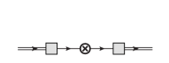
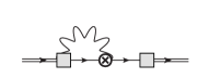
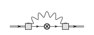
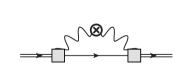
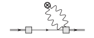
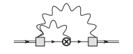
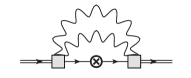
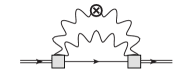
Figure 1: Diagrammatic representations of the matrix elements of the EMT. See Ref. Cao:2023ohj for more details on the evaluation of these diagrams.

The HME $t^{\alpha\beta}_{i}$ were previously evaluated up to three-body truncation (one scalar nucleon plus two scalar pions) in the non-perturbative regime in Ref. Cao:2023ohj . The relevant diagrammatic representation is shown in Fig. 1. The non-perturbative wave functions (shaded boxes) were obtained in our previous work with a Fock space expansion up to three-body $|N\rangle+|N\pi\rangle+|N\pi\pi\rangle$. A further solution up to four-body $|N\rangle+|N\pi\rangle+|N\pi\pi\rangle+|N\pi\pi\pi\rangle$ showed that the three-body truncation achieved numerical convergence Li:2014kfa ; Li:2015iaw ; Karmanov:2016yzu ; Duan:2024dhy . Summing up contributions from these diagrams, we obtain the wave function representation of the HMEs, which can be straightforwardly generalized to the $n$-body case. The wave function representation for $t_{i}^{++}$, $t^{+-}_{i}$ and $t^{12}_{i}$ are,

$$t^{++}_{i}=\, \sum_{n}\int\big{[}\mathrm{d}x_{k}\mathrm{d}^{2}r_{k\perp}\big{]}_{n}\widetilde{\psi}_{n}^{*}(\{x_{k},\vec{r}_{k\perp}\})$$ (17)

$$\times\sum_{j}x_{j}e^{i\vec{r}_{j\perp}\cdot\vec{q}_{\perp}}\widetilde{\psi}_{n}(\{x_{k},\vec{r}_{k\perp}\}),$$

$$t^{+-}_{i}=\, 2\sum_{n}\int\big{[}\mathrm{d}x_{k}\mathrm{d}^{2}r_{k\perp}\big{]}_{n}\widetilde{\psi}_{n}^{*}(\{x_{k},\vec{r}_{k\perp}\})$$ (18)

$$\times\sum_{j}e^{i\vec{r}_{j\perp}\cdot\vec{q}_{\perp}}\bigg{(}\frac{-\frac{1}{4}\tensor{\nabla}^{2}_{j\perp}+m_{j}^{2}-\frac{1}{4}q_{\perp}^{2}}{x_{j}}\bigg{)}$$

$$\times\widetilde{\psi}_{n}(\{x_{k},\vec{r}_{k\perp}\})$$

$$-\, 2\sum_{n}\int\big{[}\mathrm{d}x_{k}\mathrm{d}^{2}r_{k\perp}\big{]}_{n}\widetilde{\psi}_{n}^{*}(\{x_{k},\vec{r}_{k\perp}\})$$

$$\times e^{i\vec{r}_{n\perp}\cdot\vec{q}_{\perp}}\bigg{(}\sum_{j}\frac{-\vec{\nabla}_{j\perp}^{2}+m_{j}^{2}}{x_{j}}-M^{2}\bigg{)}$$

$$\times\widetilde{\psi}_{n}(\{x_{k},\vec{r}_{k\perp}\}),$$

$$t^{12}_{i}=\, \frac{1}{2}\sum_{n}\int\big{[}{\mathrm{d}}x_{k}{\mathrm{d}}^{2}r_{k\perp}\big{]}_{n}\widetilde{\psi}_{n}^{*}\big{(}\{x_{k},\vec{r}_{k\perp}\}\big{)}$$ (19)

$$\times\sum_{j}e^{-i\vec{q}_{\perp}\cdot\vec{r}_{j\perp}}\frac{i\tensor{\nabla}_{j1}i\tensor{\nabla}_{j2}-q_{1}q_{2}}{x_{j}}$$

$$\times\widetilde{\psi}_{n}\big{(}\{x_{k},\vec{r}_{k\perp}\}\big{)},$$

where, $f\tensor{\nabla}g=f(\vec{\nabla}g)-(\vec{\nabla}f)g$, and $j$ sums over all partons belongs to the constituent of the $i$-th type. $\big{[}\mathrm{d}x_{k}\mathrm{d}^{2}r_{k\perp}\big{]}_{n}$ is the $n$-body Fock space measure. We denote the $n$-body LFWFs as $\widetilde{\psi}_{n}(\{x_{k},\vec{r}_{k\perp}\})$ with the argument indicating the required set of constituent coordinates. See Ref. Cao:2023ohj for more details. Note that non-perturbative renormalization has been taken into account in these remarkably simple expressions, similar to the wave function representation for the electroweak current Brodsky:1998hn ; Brodsky:2000ii . The expressions for $t^{++}_{i}$ and $t^{+-}_{i}$ are previously obtained in Ref. Cao:2023ohj . Here we correct a typographical error for $t^{+-}_{i}$. It is tempting to extend the expression (19) to the full transverse stress tensor $t^{ab}_{i}$ where $a=1,2;b=1,2$. However, the $T^{12}_{i}$ operator is kinematical whereas the $T^{11}_{i}$ and $T^{22}_{i}$ operators are dynamical, and may contain spurious contributions for realistic wave functions. From Eq. (19), we obtain a general wave function representation for the Polyakov-Weiss $D$-term $D_{i}\equiv D_{i}(0)$,

$$D_{i}=\sum_{n}\int\big{[}{\mathrm{d}}x_{k}{\mathrm{d}}^{2}r_{k\perp}\big{]}_{n}\widetilde{\psi}_{n}^{*}\big{(}\{x_{k},\vec{r}_{k\perp}\}\big{)}\\ \times\sum_{j}\frac{r_{j1}\tensor{\nabla}_{j1}r_{j2}\tensor{\nabla}_{j2}-1}{x_{j}}\widetilde{\psi}_{n}\big{(}\{x_{k},\vec{r}_{k\perp}\}\big{)}.$$ (20)

IV Numerical results

From the HME of the good currents $T^{++}_{i}$, $T^{+-}_{i}$ and $T^{12}_{i}$, we are able to extract the GFFs $A_{i}$, $D_{i}$ and $\bar{c}_{i}$, where $i=N,\pi$. Note that these quantities are renormalization scheme and scale dependent. In this work, we adopt the Pauli-Villars regularization with a Pauli-Villars mass $\mu_{\textsc{pv}}=15\,\mathrm{GeV}$. In LCPT, the Pauli-Villars regularization can be converted to the $\overline{\mathrm{MS}}$ scheme Cao:2024rul . However, it is not clear how such a conversion can be done for strongly coupled scalar theory, since the $\overline{\mathrm{MS}}$ scheme is only defined in dimensional regularization in perturbation theory. Nevertheless, the GFFs $A_{i}$ and $D_{i}$ of the scalar Yukawa theory are renormalization scheme independent in the continuum limit ($\mu_{\textsc{pv}}\to\infty$).

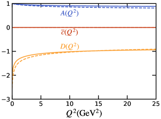
(a)  

(b)  

(c)  

Figure 2: Comparison of the gravitational form factors obtained from light-cone perturbation theory (dashed lines) and from our non-perturbative solution (solid lines) with a three-body truncation (up to one scalar nucleon and two scalar pions). The coupling is $\alpha=0.5$ and the Pauli-Villars mass $\mu_{\textsc{pv}}=15\,\mathrm{GeV}$.

Figure 2 compares the GFFs obtained from leading-order LCPT and those from our non-perturbative solution with a Fock sector truncation up to three-body (one nucleon plus two pions) at $\alpha=0.5$, where $\alpha$ is the dimensionless Yukawa coupling $\alpha=g^{2}/(16\pi m^{2})$ Li:2015iaw . As mentioned, the three-body truncation results are well converged Li:2015iaw ; Duan:2024dhy . Fig. 2(a) compares the total GFFs $A(Q^{2})$, $D(Q^{2})$ and $\bar{c}(Q^{2})$. The perturbative and non-perturbative results for $A(Q^{2})$ and $D(Q^{2})$ are in reasonable agreement. In LCPT, $\bar{c}(Q^{2})$ vanishes as expected, whereas in our non-perturbative calculation, $\bar{c}(Q^{2})$ has a small but non-vanishing value. Fig. 2(b) compares the GFF $D_{i}(Q^{2})$ obtained from LCPT and from our non-perturbative solution. Similarly, Fig. 2(c) compares the GFF $\bar{c}_{i}(Q^{2})$ obtained from LCPT and from our non-perturbative solution. While the perturbative and non-perturbative results for $A_{i}(Q^{2})$ (not shown) and $D_{i}(Q^{2})$ are in reasonable agreement as expected, GFF $\bar{c}_{i}(Q^{2})$ exhibits a visible difference between perturbative and non-perturbative results at the coupling $\alpha=0.5$. The reason is that $\bar{c}_{i}(Q^{2})$ contains a UV divergence, which magnifies the difference between the perturbative and non-perturbative results. Figures 3 and 4 present the non-perturbative results at two stronger couplings $\alpha=1.0$ and $\alpha=2.0$.

Figure 3(a) shows GFFs $A_{N}(Q^{2})$, $A_{\pi}(Q^{2})$ and their sum $A(Q^{2})$ at a non-perturbative coupling $\alpha=1.0$. As is shown in Ref. Cao:2023ohj , at large $Q^{2}$, both $A(Q^{2})$ and $A_{N}(Q^{2})$ approach the one-body limit $Z$, where $Z$ is the one-body probability, indicating a pointlike nucleon core. And $A_{\pi}(Q^{2})$ approaches zero. At small $Q^{2}$, the slope of $A_{i}(Q^{2})$ in the forward limit controls the root-mean-square (rms) matter radius $r_{Ai}^{2}=-6A^{\prime}_{i}(0)/A_{i}(0)$. At $\alpha=1.0$, the pion matter radius $r_{A,\pi}=0.51\,\mathrm{fm}$ is much larger than the nucleon matter radius $r_{A,N}=0.09\,\mathrm{fm}$, consistent with the pion cloud picture. These numbers are tabulated in Table 1 for further reference. GFFs $A_{N}(Q^{2})$, $A_{\pi}(Q^{2})$ and $A(Q^{2})$ at a larger coupling $\alpha=2.0$ are shown in Figure 4(a).

(a)  

(b)  

(c)  

Figure 3: Gravitational form factors $A_{i}(Q^{2})$, $D_{i}(Q^{2})$ and $\bar{c}_{i}(Q^{2})$ of the physical scalar nucleon, where $i=N,\pi$ for the nucleon (dashed lines) and the pion (dot-dashed lines), respectively. $A(Q^{2})=\sum_{i}A_{i}(Q^{2})$, $D=\sum_{i}D_{i}(Q^{2})$ and $\bar{c}(Q^{2})=\sum_{i}\bar{c}_{i}(Q^{2})$ are the total GFFs summing over all constituents (solid lines). The scalar Yukawa theory is solved in a light-front Hamiltonian approach with a non-perturbative coupling $\alpha=1.0$ and Pauli-Villars mass $\mu_{\textsc{pv}}=15\,\mathrm{GeV}$ in a three-body truncation (up to one scalar nucleon and two scalar pions).

Figure 3(b) shows GFFs $D_{N}(Q^{2})$, $D_{\pi}(Q^{2})$ and their sum $D(Q^{2})$ at a non-perturbative coupling $\alpha=1.0$. As is shown in Ref. Cao:2023ohj , at large $Q^{2}$, both $D(Q^{2})$ and $D_{N}(Q^{2})$ approach the one-body limit $-Z$, consistent with the existence of a pointlike nucleon core, whereas $D_{\pi}(Q^{2})$ approaches zero. At small $Q^{2}$, the slope of $D_{i}(Q^{2})$ in the forward limit controls the rms mechanical radius $r_{Di}^{2}=-6D^{\prime}_{i}(0)/D_{i}(0)$ Kumano:2017lhr . At $\alpha=1.0$, the pion mechanical radius $r_{D,\pi}=1.1\,\mathrm{fm}$ is much larger than the nucleon mechanical radius $r_{D,N}=0.15\,\mathrm{fm}$, indicating a pion cloud outside. Note that the mechanical radius is much larger than the matter radius for both the nucleon and the pion, as shown by Table 1. Similar results for $\alpha=2.0$ are shown in Figure 4(b), and listed in Table 1.

Figure 3(c) shows GFFs $\bar{c}_{N}(Q^{2})$, $\bar{c}_{\pi}(Q^{2})$ and their sum $\bar{c}(Q^{2})=\sum_{i=N,\pi}\bar{c}_{i}(Q^{2})$ extracted from $T^{12}_{i}$ and $T^{+-}_{i}$ at a non-perturbative coupling $\alpha=1.0$. Similar results for $\alpha=2.0$ are shown in Figure 4(c). Note that $\bar{c}_{N,\pi}$ is renormalization scheme and scale dependent, and we have adopted the Pauli-Villars regularization with a Pauli-Villars mass $\mu_{\textsc{pv}}=15\,\mathrm{GeV}$ as mentioned. From GFFs $A_{i},D_{i}$ and $\bar{c}_{i}$, we can obtain the individual energy density as Lorce:2017xzd ,

$$U_{i}=\, M\int\frac{{\mathrm{d}}^{2}q_{\perp}}{(2\pi)^{2}}e^{i\vec{q}_{\perp}\cdot\vec{r}_{\perp}}\Big{\{}A_{i}(q^{2}_{\perp})+\bar{c}_{i}(q_{\perp}^{2})$$ (21)

$$+\frac{q^{2}_{\perp}}{4M^{2}}\Big{[}A_{i}(q^{2}_{\perp})+D_{i}(q^{2}_{\perp})\Big{]}\Big{\}},$$

$$\equiv\, e_{i}+\Lambda_{i},$$ (22)

where, $e_{i}$ is the internal energy density and $\Lambda_{i}$ is the external stress. The total individual energy, i.e. individual energy density integrated over the transverse space, is given by the GFFs in the forward limit. From the values listed in Table 1, we obtain a mass decomposition for our strongly coupled nucleon: the nucleon d.o.f. contributes to 52% of the total mass while the contribution from the pion d.o.f. is 48% at $\mu_{\textsc{pv}}=15\,\mathrm{GeV}$ and $\alpha=1.0$. If we only consider the internal energies $e_{i}$, the bare nucleon contributes 90% and the pion cloud contributes 10%. As the coupling $\alpha$ increases, both $A_{\pi}(0)$ and $\bar{c}_{\pi}(0)$ increase and the fractional mass of the pion d.o.f. increases, and even goes beyond unity. On the other hand, the fractional internal energies remain positive and below unity.

Table 1: Gravitational form factors in the forward limit $Q^{2}=0$ as well as the related radii $r_{Ai}^{2}=-6A^{\prime}_{i}(0)/A_{i}(0)$ and $r_{Di}^{2}=-6D^{\prime}_{i}(0)/D_{i}(0)$ at selected couplings $\alpha=0.5,1.0,2.0$. For $\alpha=0.5$, we also attach light-cone perturbative theory (LCPT) results for comparison.

		$\mathrm{nucleon}$	$\mathrm{pion}$	$\mathrm{total}$
$\alpha=0.5$ (LCPT)	$r_{A}$ (fm)	$0.076$	$0.49$	$0.16$
	$r_{D}$ (fm)	$0.11$	$1.1$	$0.82$
	$A_{i}(0)$	$0.92$	$0.080$	$1.0$
	$D_{i}(0)$	$-1.2$	$-1.4$	$-2.6$
	$\bar{c}_{i}(0)$	$-0.29$	$0.29$	$0.0$
$\alpha=0.5$	$r_{A}$ (fm)	$0.061$	$0.50$	$0.13$
	$r_{D}$ (fm)	$0.11$	$1.1$	$0.75$
	$A_{i}(0)$	$0.95$	$0.050$	$1.0$
	$D_{i}(0)$	$-1.1$	$-0.97$	$-2.1$
	$\bar{c}_{i}(0)$	$-0.19$	$0.19$	$0.0$
$\alpha=1.0$	$r_{A}$ (fm)	$0.086$	$0.51$	$0.18$
	$r_{D}$ (fm)	$0.15$	$1.1$	$0.86$
	$A_{i}(0)$	$0.90$	$0.10$	$1.0$
	$D_{i}(0)$	$-1.3$	$-2.0$	$-3.2$
	$\bar{c}_{i}(0)$	$-0.38$	$0.38$	$0.0$
$\alpha=2.0$	$r_{A}$ (fm)	$0.12$	$0.53$	$0.26$
	$r_{D}$ (fm)	$0.21$	$1.1$	$0.93$
	$A_{i}(0)$	$0.81$	$0.19$	$1.0$
	$D_{i}(0)$	$-1.6$	$-4.1$	$-5.8$
	$\bar{c}_{i}(0)$	$-0.87$	$0.87$	$0.0$

The sum of GFF $\bar{c}_{i}$, $\bar{c}(Q^{2})=\sum_{i}\bar{c}_{i}(Q^{2})$, is of special interest. In the continuum limit, current conservation $\partial_{\mu}T^{\mu\nu}=0$ requires that $\bar{c}(Q^{2})$ vanishes for all $Q^{2}$, i.e. there is no external force for a self-bound system. However, in our result, $\bar{c}(Q^{2})$ is non-vanishing within the numerical precision, as shown in Figs. 3(c) and 4(c). Fortunately, the value of $\bar{c}(Q^{2})$ is small (few percent level) and scale independent, indicating that it does not contain uncanceled divergences. Furthermore, it vanishes in the forward limit $Q^{2}=0$, i.e. $\bar{c}(0)=0$, indicating that the net external force is zero, consistent with our previous analysis in Ref. Cao:2024rul .

The non-vanishing $\bar{c}(Q^{2})$ represents an isotropic spurious external force distribution on the transverse plane. For the scalar Yukawa model, the force is attractive at the center $r_{\perp}=0$ and repulsive elsewhere – the pion cloud is slightly stretched outward. Since this spurious force originates from the Fock space truncation, which implicitly breaks the Poincaré symmetry, we expect that incorporating higher Fock sector contributions would reduce its magnitude Zhang:2024 , which is already very small in the present work.

(a)  

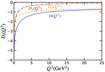
(b)  

(c)  

Figure 4: The same as Fig. 3, except with the coupling $\alpha=2.0$.

V Summary

In this work, we investigate the gravitational form factors of a strongly coupled scalar nucleon as described by the 3+1 dimensional scalar Yukawa theory. As a continuation of our previous work Cao:2023ohj , we extract the individual gravitational form factors $A_{i}(Q^{2})$, $D_{i}(Q^{2})$ and $\bar{c}_{i}(Q^{2})$ for the nucleon and the pion degrees of freedom, following the covariant analysis of the hadronic matrix element on the light front Cao:2024rul . These observables allow us to establish a coupled multi-fluid picture of the system, in which we can decompose the quantum numbers of the physical particle into the nucleon and the pion degrees of freedom. For example, the nucleon d.o.f. contributes to 52% of the physical scalar nucleon mass while the pion d.o.f. contributes to the rest 48%, at the coupling $\alpha=1.0$ and a UV resolution $\mu_{\textsc{pv}}=15\,\mathrm{GeV}$.

Our work demonstrates a systematic approach to dissect a strongly coupled quantum system in (3+1) dimensions from the underlying light-front wave functions. This approach provides not only the numbers that can be tested in experiments whenever available, but also a transparent microscopic picture of the system. While the many-body wave functions we employed in this work are relatively simple, high-quality light-front wave functions for QCD bound states are being made available with the advance of both theory and computational techniques Hornbostel:1988fb ; Vary:2009gt ; Honkanen:2010rc ; Chabysheva:2011ed ; Ji:2012ux ; Chang:2013pq ; Zhao:2014xaa ; Wiecki:2014ola ; Li:2015zda ; Lamm:2016djr ; Hiller:2016itl ; Li:2017mlw ; Tang:2018myz ; Tang:2019gvn ; Jia:2018ary ; Qian:2020utg ; Kreshchuk:2020aiq ; Kreshchuk:2020kcz ; Xu:2021wwj ; Lan:2021wok ; Ji:2021znw ; Kuang:2022vdy ; Qian:2021jxp . Methods we developed in our recent works will be useful to gain insights into hadronic structures from QCD.

References

- (1) M. V. Polyakov and P. Schweitzer, Int. J. Mod. Phys. A 33, no.26, 1830025 (2018) doi:10.1142/S0217751X18300259 [arXiv:1805.06596 [hep-ph]].
- (2) X. D. Ji, Phys. Rev. Lett. 78, 610-613 (1997) doi:10.1103/PhysRevLett.78.610 [arXiv:hep-ph/9603249 [hep-ph]].
- (3) X. D. Ji, W. Melnitchouk and X. Song, Phys. Rev. D 56, 5511-5523 (1997) doi:10.1103/PhysRevD.56.5511 [arXiv:hep-ph/9702379 [hep-ph]].
- (4) C. Lorcé, Eur. Phys. J. C 78, no.2, 120 (2018) doi:10.1140/epjc/s10052-018-5561-2 [arXiv:1706.05853 [hep-ph]].
- (5) C. Lorcé, H. Moutarde and A. P. Trawiński, Eur. Phys. J. C 79, no.1, 89 (2019) doi:10.1140/epjc/s10052-019-6572-3 [arXiv:1810.09837 [hep-ph]].
- (6) X. Ji, Y. Liu and A. Schäfer, Nucl. Phys. B 971, 115537 (2021) doi:10.1016/j.nuclphysb.2021.115537 [arXiv:2105.03974 [hep-ph]].
- (7) X. Ji, Front. Phys. (Beijing) 16, no.6, 64601 (2021) doi:10.1007/s11467-021-1065-x [arXiv:2102.07830 [hep-ph]].
- (8) C. Lorcé, A. Metz, B. Pasquini and S. Rodini, JHEP 11, 121 (2021) doi:10.1007/JHEP11(2021)121 [arXiv:2109.11785 [hep-ph]].
- (9) X. Ji and Y. Liu, Phys. Rev. D 105, no.7, 076014 (2022) doi:10.1103/PhysRevD.105.076014 [arXiv:2106.05310 [hep-ph]].
- (10) A. Freese and G. A. Miller, Phys. Rev. D 103, 094023 (2021) doi:10.1103/PhysRevD.103.094023 [arXiv:2102.01683 [hep-ph]].
- (11) A. Freese and G. A. Miller, Phys. Rev. D 104, no.1, 014024 (2021) doi:10.1103/PhysRevD.104.014024 [arXiv:2104.03213 [hep-ph]].
- (12) A. Freese and G. A. Miller, Phys. Rev. D 105, no.1, 014003 (2022) doi:10.1103/PhysRevD.105.014003 [arXiv:2108.03301 [hep-ph]].
- (13) X. Ji and Y. Liu, [arXiv:2208.05029 [hep-ph]].
- (14) A. Freese and G. A. Miller, Phys. Rev. D 108, no.3, 034008 (2023) doi:10.1103/PhysRevD.108.034008 [arXiv:2210.03807 [hep-ph]].
- (15) A. Freese and G. A. Miller, Phys. Rev. D 108, no.9, 094026 (2023) doi:10.1103/PhysRevD.108.094026 [arXiv:2307.11165 [hep-ph]].
- (16) C. Lorcé, [arXiv:2402.00429 [hep-ph]].
- (17) Y. Li, Q. Wang and J. P. Vary, [arXiv:2405.06892 [hep-ph]].
- (18) O. Teryaev, JPS Conf. Proc. 37, 020406 (2022) doi:10.7566/JPSCP.37.020406 [arXiv:2204.09742 [hep-ph]].
- (19) L. Rezzolla and O. Zanotti, Oxford University Press, 2013, ISBN 978-0-19-174650-5, 978-0-19-852890-6 doi:10.1093/acprof:oso/9780198528906.001.0001
- (20) Y. Li, W. b. Dong, Y. l. Yin, Q. Wang and J. P. Vary, Phys. Lett. B 838, 137676 (2023) doi:10.1016/j.physletb.2023.137676 [arXiv:2206.12903 [hep-ph]].
- (21) O. Teryaev, Nucl. Phys. B Proc. Suppl. 245, 195-198 (2013) doi:10.1016/j.nuclphysbps.2013.10.039 [arXiv:1309.1985 [hep-ph]].
- (22) O. V. Teryaev, Front. Phys. (Beijing) 11, no.5, 111207 (2016) doi:10.1007/s11467-016-0573-6
- (23) K. F. Liu, Phys. Lett. B 849, 138418 (2024) doi:10.1016/j.physletb.2023.138418 [arXiv:2302.11600 [hep-ph]].
- (24) F. He and I. Zahed, [arXiv:2406.07412 [nucl-th]].
- (25) A. Metz, B. Pasquini and S. Rodini, Phys. Rev. D 102, 114042 (2020) doi:10.1103/PhysRevD.102.114042 [arXiv:2006.11171 [hep-ph]].
- (26) V. D. Burkert, L. Elouadrhiri, F. X. Girod, C. Lorcé, P. Schweitzer and P. E. Shanahan, Rev. Mod. Phys. 95, no.4, 041002 (2023) doi:10.1103/RevModPhys.95.041002 [arXiv:2303.08347 [hep-ph]].
- (27) X. Cao, Y. Li and J. P. Vary, Phys. Rev. D 108, no.5, 056026 (2023) doi:10.1103/PhysRevD.108.056026 [arXiv:2308.06812 [hep-ph]].
- (28) Y. Li, V. A. Karmanov, P. Maris and J. P. Vary, Few Body Syst. 56, no.6-9, 495-501 (2015) doi:10.1007/s00601-015-0965-0 [arXiv:1411.1707 [nucl-th]].
- (29) Y. Li, V. A. Karmanov, P. Maris and J. P. Vary, Phys. Lett. B 748, 278-283 (2015) doi:10.1016/j.physletb.2015.07.014 [arXiv:1504.05233 [nucl-th]].
- (30) V. A. Karmanov, Y. Li, A. V. Smirnov and J. P. Vary, Phys. Rev. D 94, no.9, 096008 (2016) doi:10.1103/PhysRevD.94.096008 [arXiv:1610.03559 [hep-th]].
- (31) S. D. Drell and T. M. Yan, Phys. Rev. Lett. 24, 181-185 (1970) doi:10.1103/PhysRevLett.24.181
- (32) G. B. West, Phys. Rev. Lett. 24, 1206-1209 (1970) doi:10.1103/PhysRevLett.24.1206
- (33) S. J. Brodsky and S. D. Drell, Phys. Rev. D 22, 2236 (1980) doi:10.1103/PhysRevD.22.2236
- (34) S. J. Brodsky and D. S. Hwang, Nucl. Phys. B 543, 239-252 (1999) doi:10.1016/S0550-3213(98)00807-4 [arXiv:hep-ph/9806358 [hep-ph]].
- (35) S. J. Brodsky, D. S. Hwang, B. Q. Ma and I. Schmidt, Nucl. Phys. B 593, 311-335 (2001) doi:10.1016/S0550-3213(00)00626-X [arXiv:hep-th/0003082 [hep-th]].
- (36) S. J. Brodsky, H. C. Pauli and S. S. Pinsky, Phys. Rept. 301, 299-486 (1998) doi:10.1016/S0370-1573(97)00089-6 [arXiv:hep-ph/9705477 [hep-ph]].
- (37) X. Cao, S. Xu, Y. Li, G. Chen, X. Zhao, V. A. Karmanov and J. P. Vary, JHEP 07, 095 (2024) doi:10.1007/JHEP07(2024)095 [arXiv:2405.06896 [hep-ph]].
- (38) S. S. Chabysheva and J. R. Hiller, Phys. Rev. D 82, 034004 (2010) doi:10.1103/PhysRevD.82.034004 [arXiv:1006.1077 [hep-ph]].
- (39) J. R. Hiller, Prog. Part. Nucl. Phys. 90, 75-124 (2016) doi:10.1016/j.ppnp.2016.06.002 [arXiv:1606.08348 [hep-ph]].
- (40) X. D. Ji, Phys. Rev. Lett. 74, 1071-1074 (1995) doi:10.1103/PhysRevLett.74.1071 [arXiv:hep-ph/9410274 [hep-ph]].
- (41) X. D. Ji, Phys. Rev. D 52, 271-281 (1995) doi:10.1103/PhysRevD.52.271 [arXiv:hep-ph/9502213 [hep-ph]].
- (42) P. A. M. Dirac, Rev. Mod. Phys. 21, 392-399 (1949) doi:10.1103/RevModPhys.21.392
- (43) J. Carbonell, B. Desplanques, V. A. Karmanov and J. F. Mathiot, Phys. Rept. 300, 215-347 (1998) doi:10.1016/S0370-1573(97)00090-2 [arXiv:nucl-th/9804029 [nucl-th]].
- (44) Y. Duan, S. Xu, S. Cheng, X. Zhao, Y. Li and J. P. Vary, [arXiv:2404.07755 [hep-ph]].
- (45) S. Kumano, Q. T. Song and O. V. Teryaev, Phys. Rev. D 97, no.1, 014020 (2018) doi:10.1103/PhysRevD.97.014020 [arXiv:1711.08088 [hep-ph]].
- (46) K. Hornbostel, S. J. Brodsky and H. C. Pauli, Phys. Rev. D 41, 3814 (1990) doi:10.1103/PhysRevD.41.3814
- (47) J. P. Vary, H. Honkanen, J. Li, P. Maris, S. J. Brodsky, A. Harindranath, G. F. de Teramond, P. Sternberg, E. G. Ng and C. Yang, Phys. Rev. C 81, 035205 (2010) doi:10.1103/PhysRevC.81.035205 [arXiv:0905.1411 [nucl-th]].
- (48) H. Honkanen, P. Maris, J. P. Vary and S. J. Brodsky, Phys. Rev. Lett. 106, 061603 (2011) doi:10.1103/PhysRevLett.106.061603 [arXiv:1008.0068 [hep-ph]].
- (49) S. S. Chabysheva and J. R. Hiller, Phys. Lett. B 711, 417-422 (2012) doi:10.1016/j.physletb.2012.04.032 [arXiv:1103.0037 [hep-ph]].
- (50) C. R. Ji and A. T. Suzuki, Phys. Rev. D 87, no.6, 065015 (2013) doi:10.1103/PhysRevD.87.065015 [arXiv:1212.2265 [hep-th]].
- (51) L. Chang, I. C. Cloet, J. J. Cobos-Martinez, C. D. Roberts, S. M. Schmidt and P. C. Tandy, Phys. Rev. Lett. 110, no.13, 132001 (2013) doi:10.1103/PhysRevLett.110.132001 [arXiv:1301.0324 [nucl-th]].
- (52) X. Zhao, H. Honkanen, P. Maris, J. P. Vary and S. J. Brodsky, Phys. Lett. B 737, 65-69 (2014) doi:10.1016/j.physletb.2014.08.020 [arXiv:1402.4195 [nucl-th]].
- (53) P. Wiecki, Y. Li, X. Zhao, P. Maris and J. P. Vary, Phys. Rev. D 91, no.10, 105009 (2015) doi:10.1103/PhysRevD.91.105009 [arXiv:1404.6234 [nucl-th]].
- (54) Y. Li, P. Maris, X. Zhao and J. P. Vary, Phys. Lett. B 758, 118-124 (2016) doi:10.1016/j.physletb.2016.04.065 [arXiv:1509.07212 [hep-ph]].
- (55) H. Lamm and R. Lebed, Phys. Rev. D 94, no.1, 016004 (2016) doi:10.1103/PhysRevD.94.016004 [arXiv:1606.06358 [hep-ph]].
- (56) Y. Li, P. Maris and J. P. Vary, Phys. Rev. D 96, 016022 (2017) doi:10.1103/PhysRevD.96.016022 [arXiv:1704.06968 [hep-ph]].
- (57) S. Tang, Y. Li, P. Maris and J. P. Vary, Phys. Rev. D 98, no.11, 114038 (2018) doi:10.1103/PhysRevD.98.114038 [arXiv:1810.05971 [nucl-th]].
- (58) S. Tang, Y. Li, P. Maris and J. P. Vary, Eur. Phys. J. C 80, no.6, 522 (2020) doi:10.1140/epjc/s10052-020-8081-9 [arXiv:1912.02088 [nucl-th]].
- (59) S. Jia and J. P. Vary, Phys. Rev. C 99, no.3, 035206 (2019) doi:10.1103/PhysRevC.99.035206 [arXiv:1811.08512 [nucl-th]].
- (60) W. Qian, S. Jia, Y. Li and J. P. Vary, Phys. Rev. C 102, no.5, 055207 (2020) doi:10.1103/PhysRevC.102.055207 [arXiv:2005.13806 [nucl-th]].
- (61) M. Kreshchuk, S. Jia, W. M. Kirby, G. Goldstein, J. P. Vary and P. J. Love, Phys. Rev. A 103, no.6, 062601 (2021) doi:10.1103/PhysRevA.103.062601 [arXiv:2011.13443 [quant-ph]].
- (62) M. Kreshchuk, S. Jia, W. M. Kirby, G. Goldstein, J. P. Vary and P. J. Love, Entropy 23, no.5, 597 (2021) doi:10.3390/e23050597 [arXiv:2009.07885 [quant-ph]].
- (63) S. Xu et al. [BLFQ], Phys. Rev. D 104, no.9, 094036 (2021) doi:10.1103/PhysRevD.104.094036 [arXiv:2108.03909 [hep-ph]].
- (64) J. Lan et al. [BLFQ], Phys. Lett. B 825, 136890 (2022) doi:10.1016/j.physletb.2022.136890 [arXiv:2106.04954 [hep-ph]].
- (65) Z. Kuang et al. [BLFQ], Phys. Rev. D 105, no.9, 094028 (2022) doi:10.1103/PhysRevD.105.094028 [arXiv:2201.06428 [hep-ph]].
- (66) W. Qian, R. Basili, S. Pal, G. Luecke and J. P. Vary, Phys. Rev. Res. 4, no.4, 043193 (2022) doi:10.1103/PhysRevResearch.4.043193 [arXiv:2112.01927 [quant-ph]].
- (67) Wenyu Zhang, Yang Li, and James Vary, in prepration.