Safe Adaptive Control for Uncertain Systems with Complex Input Constraints

Abstract

In this paper, we propose a novel adaptive Control Barrier Function (CBF) based controller for nonlinear systems with complex, time-varying input constraints. Conventional CBF approaches often struggle with feasibility issues and stringent assumptions when addressing input constraints. Unlike these methods, our approach converts the input-constraint problem into an output-constraint CBF design. This transformation simplifies the Quadratic Programming (QP) formulation and enhances compatibility with the CBF framework. We design an adaptive CBF-based controller to manage the mismatched uncertainties introduced by this transformation. Our method systematically addresses the challenges of complex, time-varying, and state-dependent input constraints. The efficacy of the proposed approach is validated using numerical examples.

I Introduction

In practical control system design, input constraints are unavoidable. These constraints may arise from various sources, including actuator limitations and performance requirements. Violating these constraints can lead to performance degradation, hazards, or system damage [1, 2].

Over the past few decades, addressing input constraints in controller design has garnered significant attention due to both practical needs and theoretical challenges. Model Predictive Control (MPC) has been a prominent method for managing constraints [3]. Several studies have investigated its application in handling input constraints in nonlinear systems. However, nonlinear MPC requires solving a nonlinear programming (NLP) problem, which is not always feasible for online applications due to the limitations of QP solvers in low-dimensional parameter spaces [4, 5]. Alternatively, the reference governor (RG) approach [6] integrates input constraints into a well-designed nominal controller using QP. Despite its effectiveness, RG necessitates the computation of admissible sets, complicating its implementation [7]. Barrier Lyapunov Function (BLF) based approaches have also been widely adopted to manage constraints in various nonlinear systems. For instance, BLF-based controllers have been proposed for systems with input saturation [8, 9]. However, BLFs primarily address time-varying constraints and often overlook the more complex scenario of state-dependent constraints. This focus on time-based constraints limits their applicability in systems where the state and environment can change unpredictably [10, 11]. Furthermore, BLF methods typically require the reference trajectory to remain within the constraint set, adding complexity to the design process and potentially restricting system performance [12, 13].

Recently, control barrier functions (CBFs) have emerged as an effective tool for managing constraints in control systems [14, 15]. In CBF-based approaches, constraints on system outputs are typically addressed through Quadratic Programming (QP) and integrated with the control Lyapunov function, resulting in the CBF-CLF-QP framework. This framework enables the real-time handling of safety-critical constraints effectively.

However, the application of CBF-based designs to systems with input constraints is limited. One method to address this is through integral control barrier functions (ICBFs)[16]. While promising, further theoretical investigation is needed to establish the feasibility of ICBF-based controllers[17], as highlighted in Remark 4 of [16]. Another approach involves incorporating input saturation directly into the QP formulation. In [18], input constraints are defined as one of the multiple CBF conditions in the QP formulation. Although this approach has been successful in certain specific models, introducing multiple constraints in the QP could potentially lead to infeasibility issues [19]. To address these challenges, various studies have proposed methods that rely on certain assumptions. For example, in [20], the authors assume that the safety regions of multiple CBFs do not conflict, which allows each CBF to be treated independently. However, this assumption is often unrealistic in practical scenarios. In [21], a multiple CBF-based approach for robot navigation is proposed, but it relies on a specifically structured environment. These assumptions can simplify the problem but do not fully resolve the underlying challenges of handling input constraints with CBFs. Consequently, managing input constraints in CBF-based control designs remains a complex and unresolved issue.

In this research, we propose an adaptive CBF-based scheme for input-constrained nonlinear systems, where constraint boundaries are related to both state and time. Instead of incorporating the input constraint directly into the QP formulation, we transform the input-constrained problem into an output-constrained one. This transformation reduces the number of constraints in the QP formulation and aligns better with the solid CBF framework [22]. Specifically, we introduce integrator dynamics to the control signal, creating an auxiliary state variable. This converts the original system into an augmented system with output constraints. While this transformation simplifies the control problem and enhances compatibility with the CBF framework, it also introduces mismatched uncertainty into the original system (see Section IV). We address this issue by designing an adaptive CBF-based controller. Our approach systematically mitigates the challenges posed by complex, time-varying input constraints, ensuring reliable operation under varying conditions. Additionally, it enhances system robustness and performance by employing an adaptive CBF to handle system uncertainties effectively.

The rest of the paper is organized as follows. In Section II, some preliminaries about CLF, Functions approximation technique (FAT), and CBF are introduced. In Section III, a safe adaptive input-constraint problem is stated for an $n$th order nonlinear system, and a corresponding input-constraint control algorithm is developed based on the CBF technique. The proposed control the algorithm is verified under simulations in Section IV, and finally, conclusions are drawn in Section V.

II Preliminary

In this section, the concepts of FAT and CBF are reviewed, which are the main tools for our controller design.

II-A Notation

We denote the set of real numbers $\mathbb{R}$ and non-negative reals $\mathbb{R}_{+}.$ A continuous function $\alpha:[0,a)\to[0,\infty)$ is class- $\mathcal{K}$ if it is strictly increasing on the domain, and $\alpha(0)=0$. It is class-$\mathcal{K}_{\infty}$ if $\lim_{r\to\infty}\alpha(r)\to\infty$ .The Lie derivative of $h(x)$ along $f(x)$ is denoted $L_{f}h(x)=\frac{dh}{dx}f(x).$ The short hand $\dot{h}(x)=\frac{dh}{dx}\dot{x}$ will also be used to indicate time derivatives of $h$ along flows from a state $x.$

II-B CLF and CBF

Consider the following control affine system: [22]

$$\dot{x}(t)=f(x(t))+g(x(t))u(t)$$ (1)

where $x(t)=\begin{bmatrix}x_{1}(t),\ldots,x_{n}(t)\end{bmatrix}^{\top}\in\mathbb{R}^{n}$ is the state vector, $u(t)\in\mathbb{R}^{m}$ is a constrained control input, and $f:\mathbb{R}^{n}\to\mathbb{R}^{n}$ and $g:\mathbb{R}^{n}\to\mathbb{R}^{n\times m}\setminus\{{0}\}$ are smooth continuous and local Lipschitz functions. In the rest of the preliminary, we omit time $t$ for $x$ and $u$, as the references stated, provided no confusion arises.

Definition 1.

[23] A smooth function $V:\mathbb{R}^{n}\to\mathbb{R}_{+}$ is a control Lyapunov function (CLF) for system (1) if there exist $\alpha_{1}$, $\alpha_{2}$ and $\alpha_{3}\in\mathcal{K}_{\infty}$ such that:

$$\alpha_{1}(\lVert x\rVert)\leq V(x) \leq\alpha_{2}(\lVert x\rVert)$$ (2)

$$\inf_{u\in\mathbb{R}^{m}}\left[\mathcal{L}_{f}V(x)+\mathcal{L}_{g}V(x)u\right] \leq-\alpha_{3}(\lVert x\rVert)$$

for all $x\in\mathbb{R}^{n}$, where $\mathcal{L}_{f}V({x})=\frac{\partial V}{\partial x}f(x)$ and $\mathcal{L}_{g}V({x})=\frac{\partial V}{\partial x}g(x)$ are the Lie derivatives.

This definition means that there exists a set of stabilizing controls that renders the origin globally asymptotically stable. This set is defined by

$$K_{\text{clf}}(x)\!=\!\left\{u\in\mathbb{R}^{m}:\mathcal{L}_{f}V(x)+\mathcal{L}_{g}V(x)u{\leq}-\alpha_{3}(\lVert x\rVert)\right\}.$$ (3)

Safety can be framed in the context of enforcing invariance of a particular set of states. Consider control system (1) and suppose there exists a set $\mathcal{C}\subset\mathbb{R}^{n}$ defined as the 0-superlevel set of a continuously differentiable function $h:\mathbb{R}^{n}\to\mathbb{R}$, as follows:

$$\mathcal{C}=\{x\in\mathbb{R}^{n}:h(x)\geq 0\}.$$ (4)

The set $\mathcal{C}$ is referred to as the safe set, which we assume this set is closed, non-empty, and simply connected.

Definition 2.

The set $\mathcal{C}$ is called forward controlled invariant with respect to system (1) if for every $x_{0}\in\mathcal{C}$, there exists a control signal $u(t)$ such that $x(t;t_{0},x_{0})\in\mathcal{C}$ for all $t\geq t_{0}$, where $x(t;t_{0},x_{0})$ denotes the solution of (1) at time $t$ with initial condition $x_{0}\in\mathbb{R}^{n}$ at $t=t_{0}$.

Definition 3.

Let $\mathcal{C}\in\mathbb{R}^{n}$ be defined in Definition 2. The function $h$ is called a (zeroing) CBF if there exists a constant $\gamma_{h}>0$ such that

$$\sup_{{u}\in\mathbb{R}^{m}}\left[\mathcal{L}_{f}h({x})+\mathcal{L}_{g}h({x}){u}+\gamma_{h}h({x})\right]\geq 0$$ (5)

for all $x\in\mathbb{R}^{n}$, where, $\mathcal{L}_{f}h({x})=\frac{\partial h}{\partial x}f(x)$ and $\mathcal{L}_{g}h({x})=\frac{\partial h}{\partial x}g(x)$ are the Lie derivatives. Given a CBF $h$, the set of all control values that satisfy (5) for all $x\in\mathbb{R}^{n}$ is defined as

$$K_{\text{cbf}}(x)=\{u\in\mathbb{R}^{m}:\mathcal{L}_{f}h({x})+\mathcal{L}_{g}h({x}){u}+\gamma_{h}h({x})\geq 0\}.$$ (6)

It was proven in [22] that any Lipschitz continuous controller $u$ satisfying $u(x)\in K_{\text{cbf}}(x)$ for every $x\in\mathbb{R}^{n}$ guarantees the forward invariance of $\mathcal{C}$. The provably safe control law is obtained by solving an online quadratic program (QP) problem that includes the control barrier condition as its constraint.

II-C Projection operator

To compensate for the effects of the uncertainty $d_{j}$ by FAT (20), a projection method [24],  [25] is always adopted in the consequent design of adaptive laws. The projection operator is defined as

$$\mathrm{Proj}({x},{y},l(x))$$ (7)

$$=\begin{cases}{y}-l({x})\frac{\nabla l({x})\nabla l({x})^{\top}}{\|\nabla l({x})\|^{2}}{y},&\mathrm{if\leavevmode\nobreak\ }l({x})>0\wedge{y}^{\top}\nabla l({x})>0,\\ {y},&\mathrm{otherwise}.\end{cases}$$

Here ${x}$, ${y}$ are arbitrary vectors and $l({x})$ is convex function defined as

$$l({x})=\frac{{x}^{\top}{x}-\bar{x}^{2}}{2\eta\bar{x}+\eta^{2}},$$ (8)

where $\bar{x}$ and $\eta$ are constants.

Lemma 1.

[25] Let ${x}^{*}\in\mathbb{R}^{n}$ be arbitrary, if $x\in\mathbb{R}^{n}$ satisfies $l({x})\leq 0$,then

$$({x}-{x}^{*})^{\top}(\mathrm{Proj}({x},{y},l(x))-{y})\leq 0.$$ (9)

III Problem statement

In this section, we explore how CBFs can be used to achieve input-constrained safety for the system (1) with uncertainty. Firstly, we consider a nonlinear control-affine dynamical system with uncertainty

$$\dot{x}(t) =f(x(t))+g(x(t))u(t)+d_{x}(t),$$ (10)

where, $d_{x}(t)\in\mathcal{D}\subset\mathbb{R}^{n}$ is an unknown uncertainty of time $t$ such that $d_{x}(t)\in\mathcal{D}$ for all $t$ for a subset $\mathcal{D}$ of $\mathbb{R}^{n}$. We denote the initial state and control input of the system at time $t=0$ by $x_{0}$ and $u_{0}$, respectively, i.e., $x(0)=x_{0}$, $u(0)=u_{0}$. We introduce $\kappa(x(t),t)$, a time-varying continuous scalar function that depends on $x$ and $t$, as the input constraint:

$$\lVert u(t)\rVert\leq\kappa(x(t),t),$$ (11)

for all $t\geq 0$. The magnitude of the control input is expected to be kept within limits imposed by the actuator’s saturation constraints. However, current BLF-based methods commonly involve the feasibility conditions on constraint set. Specifically, when the time-varying saturation includes an unfeasible region will pose difficulty for control safety, as in Example 1:

Example 1.

We consider a simple but representative case of (10):

$$\dot{x}_{1}(t) =x_{2}(t),$$ (12)

$$\dot{x}_{2}(t) =u(t),$$

where $u(t)\in\mathcal{U}\subset\mathbb{R}$ is the control input subjected to a closed control constraint set defined as

$$\mathcal{U}=\{u\colon[0,\infty)\!\to\!\mathbb{R}^{m}:\underline{k}_{l}(t)\leq u(t)\leq\overline{k}_{h}(t)\},$$ (13)

for all $t\geq 0$, where, $\underline{k}_{l}:\mathbb{R}_{+}\to\mathbb{R}$ and $\overline{k}_{h}:\mathbb{R}_{+}\to\mathbb{R}$ are the lowest and highest levels of input constraint such that $\underline{k}_{l}(t)<\overline{k}_{h}(t)$ for all $t\geq 0$. We designed a symmetric time-varying constraint as

$$\underline{k}_{l}(t) =-\sin(t)-1,$$

$$\overline{k}_{h}(t) =\sin(t)+1.$$ (14)

For the system in Example 1, to implement the input-constraint via barrier-function-based methods, we refer to a solid barrier function in [9] as

$$\mathcal{B}(t)\!=\!b(u;\underline{k}_{l},\overline{k}_{h})\!=\!\operatorname{log}\left(\frac{\overline{k}_{h}(t)}{\underline{k}_{l}(t)}\frac{\underline{k}_{l}(t)\!-\!u(t)}{\overline{k}_{h}(t)\!-\!u(t)}\right),$$ (15)

where $b:\mathbb{R}\to\mathbb{R}$ is the barrier function defined on $(\underline{k}_{l},\overline{k}_{h})$, as it is obviously to see, if $u$ approaches the boundaries of the permitted range $(\underline{k}_{l},\overline{k}_{h})$, $\mathcal{B}$ will approach infinity, i.e., $\lim_{u\to\underline{k}_{l}^{+}}b(u;\underline{k}_{l},\overline{k}_{h})=-\infty$, or $\lim_{u\to\overline{k}_{h}^{-}}b(u;\underline{k}_{l},\overline{k}_{h})=+\infty$. Note that $\inf_{t}\{\overline{k}_{h}(t)\}=0$ and $\sup_{t}\{\underline{k}_{l}(t)\}=0$, one can always find $t_{0}$ such that

$$\exists t_{0}>0:(u_{\sup}(t_{0})=0\lor u_{\inf}(t_{0})=0),$$ (16)

and we define the set $T_{0}$ that $t$ satisfies (16) as

$$T_{0}=\{t\in\mathbb{R}^{+}:u_{\sup}(t)=0\lor u_{\inf}(t)=0\}.$$ (17)

Therefore, for $t\geq 0$, $t\notin T_{0}$, $\mathcal{B}$ is bounded, then input constraints (13) are automatically satisfied. However, for $t\in T_{0}$, then $\overline{k}_{h}(t)=0$ or $\underline{k}_{l}(t)=0$, and obviously $\mathcal{B}(t)$ diverges. Therefore under any $u(t)\in\mathcal{U}$, closed-loop trajectories will leave safe set. Thus $\mathcal{B}$ cannot be rendered forward invariant under the input constraints.

To address such an unsafe condition, and guarantee the input constraint, we define an input constraint safe set for system (10) based on the CBF technique. One defines a Lipschitz continuous function $h$ as a barrier function

$$h(x,u,t)=-u(t)^{\top}u(t)+\kappa^{2}(x,t)$$ (18)

and to guarantee the input constraint, we let a safe set $\mathcal{C}_{u}$ for actual control input $u$ as

$$\mathcal{C}_{u}=\{u(t)\in\mathbb{R}^{m},h(x,u,t)\geq 0\}.$$ (19)

The FAT is an effective tool for dealing with control systems with time-varying nonlinear uncertainties. For instance, let $d(t)$ be an unknown time-varying function in a control system. One can utilize weighted basis functions to represent $d(t)$ at each time instant, as shown in [24], [25]:

$${d}(t)=\sum_{i=1}^{\infty}{w}_{i}\psi_{h,j}(t)$$ (20)

where $w_{i}$ denotes an unknown constant vector (weight) and $\psi_{h,j}(t)$ is the basis function to be selected. It is a common practice to design an adaptive law that approximates the weights $w_{i}$ to mitigate the impact of $d(t)$ on the control system. Several candidates for the basis function $\psi_{h,j}(t)$ in(20) can be chosen to approximate the nonlinear functions. In this paper, we select the same form of $\psi_{h,j}$ as in[25]. This preliminary framework sets the stage for the design of the specific adaptive law, which will be detailed in the subsequent sections.

Assumption 1.

The FAT of $d(t)$ in (20) satisfies $\lVert w_{i}\rVert\leq\bar{w}_{i}$ for a constant $w_{i}$, and $\bar{w}_{i}$ is a known positive constant.

Now, we can state the main objective of this paper:

Problem 1.

Given the system (10), design a feedback controller $u(t)$ such that for any $u_{0}\in\mathcal{C}_{u}$, the closed-loop trajectories of (10) satisfy $\lim_{t\to\infty}x(t)\to 0$ and $u(t)\in\mathcal{C}_{u}$ for all $t\geq 0$.

IV Control barrier function based input constraints

In this section, we design our CBF-based input-constrained controller. First, we introduce an auxiliary control input to transform the original system into an augmented system, thereby converting the original input constraint problem into an output-constrained problem. Next, we propose an adaptive CBF-based method to ensure the safety of input constraints. Finally, we demonstrate that combining this safety controller with a stabilizing nominal control law through a quadratic program achieves the desired behavior, as outlined in our problem statement.

IV-A Auxiliary transformation

To provide time-varying bounds on the actual control variable $u$, it is natural to place an integrator in the feedback path to augment the system’s output as the input of an auxiliary system. This transforms the original system into a class of uncertain nonlinear systems given by:

$$\dot{x}(t) =f(x(t))+g(x(t))u(t)+d_{x}(t),$$

$$\dot{u}(t) =v(t)+d_{u}(t),$$ (21)

where $d_{x}(t)\in\mathcal{D}\subset\mathbb{R}^{n}$ and $d_{u}(t)\in\mathcal{D}\subset\mathbb{R}^{n}$ are uncertainties of time $t$, and $v(t)\in\mathbb{R}^{m}$ is an auxiliary input defined as:

$$v(t)=\phi(t)+\mu(t),$$ (22)

where $\phi(t)\in\mathbb{R}^{m}$ is the auxiliary dynamics (IV-A), and $\mu(t)\in\mathbb{R}^{m}$ is the safety controller represents the difference between auxiliary input $v$ and nominal control $\phi$. We refer to system (IV-A) as the nominal system when $\mu(t)=0$ for all $t\geq 0$.

Remark 1.

The uncertainty in the system (IV-A) will always be regarded as sensor faults polluting all the states [26]. The pollution caused by such sensor faults cannot be separated from the real signal, thus being mixed into the feedback signal and processed by the algorithm. Thus we address such a scenario that all the states including $u$ are polluted due to sensor faults coinciding in each system state, which is of theoretical and practical significance.

The following proposition gives an adaptive form of CLF for system (IV-A). Explicit time dependence of variable $t$ is omitted in the rest of this paper when it is clear from the context.

Proposition 1.

Suppose $\mu(t)=0$ for all $t\geq 0$ in system (IV-A), and there exist a continuously differentiable function $V_{0}:\mathbb{R}^{n}\to\mathbb{R}_{\geq 0}$ and a legacy feedback controller $u_{d}(x,\hat{w}_{x})\in\mathbb{R}^{m}$ for system (IV-A), where $\hat{w}_{x}$ is an adaptive law designed later. If $u_{d}(0)=0$ and

$$\gamma_{1}(\|{x},\hat{w}_{x}\|)\leq V_{0}({x,\hat{w}_{x}})\leq\gamma_{2}(\|{x},\hat{w}_{x}\|),$$ (23)

$$L_{\tilde{f}_{clf}}V_{0}(x,\!\hat{w}_{x})\!+\!L_{g}V_{0}(x,\!\hat{w}_{x})u_{d}(x,\hat{w}_{x})\!\leq\!\ \gamma_{3}(\|{x}\|),$$ (24)

for all $x\in\mathbb{R}^{n}$, where $\gamma_{1}$ , $\gamma_{2}$, $\gamma_{3}$ are class $\mathcal{K}_{\infty}$ functions, and $\tilde{f}_{clf}$ is defined by

$$\tilde{f}_{clf}(x,\hat{w}_{x})=f(x)+d_{x}-\hat{w}_{x}.$$ (25)

Defining a function $V:\mathbb{R}^{n}\times\mathbb{R}^{m}\to\mathbb{R}_{\geq 0}$ as

$$V(x,u,\hat{w}_{x},\hat{w}_{u}) \!=\!V_{0}(x,\hat{w}_{x})\!+\!(d_{u}\!-\!\hat{w}_{u})^{\top}(d_{u}\!-\!\hat{w}_{u})$$

$$\quad\!+\!(u\!-\!u_{d}(x,\hat{w}_{x}))^{\top}(u\!-\!u_{d}(x,\hat{w}_{x})),$$ (26)

where $\hat{w}_{u}$ is another adaptive law similar to $\hat{w}_{x}$. We further suppose that $u_{d}$ in (24) and $\phi$ in (IV-A) can be designed such that

$$\dot{V}(x,u,v,\hat{w}_{x},\hat{w}_{u})\leq-\gamma_{3}(\|{x}\|)-\gamma_{4}(\|u-u_{d}(x,\hat{w}_{x})\|),$$ (27)

where $\gamma_{4}$ is a class $\mathcal{K}_{\infty}$ function. Then $V$ in (27) is a CLF for system (IV-A).

Proof.

The proof follows directly from the assumptions and the definition of CLF on Definition 1. Since $V_{0}$ satisfies the given inequalities and $u_{d}$ stabilizes the system (IV-A), the constructed function $V$ inherits these properties, establishing $V$ as a control Lyapunov function for system (IV-A). Furthermore, we have:

$$\inf_{v\in\mathbb{R}^{n}}\!\dot{V}\!(x,\!u,\!v,\!\hat{w}_{x},\!\hat{w}_{u})\!<\!-\!\gamma_{3}(\|{x}\|)\!-\!\gamma_{4}(\|u\!-\!u_{d}(x,\!\hat{w}_{x})\|),$$ (28)

for all $x\neq 0$ and $u\neq u_{d}$. Hence, $V$ is a CLF for the system. ∎

Suppose a valid control barrier function $h(u,\kappa)$ is associated with the input constraint set $\mathcal{C}_{u}$. Then from Definition 3 and Lemma 1, a safe CLF-CBF-QP-based optimization problem for system (IV-A) could be defined as follows:

$$\underset{\mu\in\mathbb{R}^{m}}{\min}\quad\|\mu\|$$ (29)

$$\mathrm{s.t.}$$

$$\dot{V}(x,u,v,\hat{w}_{x},\hat{w}_{u})\!<\!-\!\gamma_{3}(\|{x}\|)\!-\!\gamma_{4}(\|u-u_{d}(x,\hat{w}_{x})\|),$$

$$L_{f}h(u,\kappa)\!+\!L_{g}h(u,\kappa)v\!\geq\!\gamma_{h}(h(u,\kappa)),$$

where $\gamma_{h}$ is a class $\mathcal{K}_{\infty}$ function ensuring the input constraint.

The following two steps will be introduced to derive the inequality constraints in (29). Firstly, we design a nominal controller $\phi$ for the stability of the nominal system, as the CLF inequality constraint shown in (29). Then unifying this stability condition with CBF safety condition (19), as the second inequality constraint in (29), then solved by QP optimization [27].

IV-B CLF inequality constraint

To compensate for the effects of time-varying uncertainty $d_{x}$ and $d_{u}$ in system (IV-A), using FAT approach, the approximation of system (IV-A) can be represented as

$$\dot{x} =f+gu+\sum_{i=1}^{N}w_{x,i}\psi_{x,i},$$ (30)

$$\dot{u} =\phi+\mu+\sum_{i=1}^{N}w_{u,i}\psi_{u,i},$$

where $N$ is the number of basis functions used in the approximation. $w_{x,i}$ and $w_{u,i}$ denotes the unknown constant vector, $\psi_{x,i}(t)$ and $\psi_{u,i}(t)$ are the basis functions to be selected.

The following theorem shows that we can construct a feedback controller $\phi$ to locally achieve the CLF inequality constraint (28) which stated in Proposition 1

Theorem 2.

Define the nominal control $\phi$ in system (30) as

$$\begin{multlined}\phi=\dfrac{1}{g}\Big{(}-\dot{f}-\sum_{i=1}^{N}\hat{w}_{u,i}\psi_{u,i}-\dfrac{c_{x}}{\theta_{x}}(f+gu)\\ \quad-\dot{g}(x)u-\dfrac{c_{u}}{\theta_{u}}\Big{(}u+\sum_{i=1}^{N}\hat{w}_{x,i}\psi_{x,i}+c_{x}\dfrac{x}{\theta_{x}}\Big{)}\Big{)}.\end{multlined}\phi=\dfrac{1}{g}\Big{(}-\dot{f}-\sum_{i=1}^{N}\hat{w}_{u,i}\psi_{u,i}-\dfrac{c_{x}}{\theta_{x}}(f+gu)\\ \quad-\dot{g}(x)u-\dfrac{c_{u}}{\theta_{u}}\Big{(}u+\sum_{i=1}^{N}\hat{w}_{x,i}\psi_{x,i}+c_{x}\dfrac{x}{\theta_{x}}\Big{)}\Big{)}.$$ (31)

where $c_{x}$, $c_{u}$ and $\theta_{x}$, $\theta_{u}$ are positive constants, $\hat{w}_{x,i}$ is the adaptive law and $\hat{w}_{u,i}$ is the update law given by

$$\dot{\hat{W}}_{xi} =\lambda_{x}^{-1}\psi_{x,i}x,$$

$$\dot{\hat{W}}_{ui} =\lambda_{u}^{-1}\psi_{u,i}s_{u}$$

$$=\lambda_{u}^{-1}\psi_{u,i}\left(f+gu+\sum_{i=1}^{N}\hat{w}_{x,i}\psi_{x,i}+c_{x}\dfrac{x}{\theta_{x}}\right).$$ (32)

Then, all closed-loop system signals in (30) are bounded and $\lim_{t\to\infty}x(t)=0$.

Proof.

To guarantee the stability of the nominal system, in the rest of this section, we assume $\mu(t)=0$ for all $t>0$ in (22). We further define the sliding surface as

$$s_{x} =x-x_{d},$$

$$s_{u} =f+gu-u_{d},$$ (33)

where $x_{d}$ and $u_{d}$ represent the desired value of state $x$ and $u$ follows

$$x_{d} =0,$$

$$u_{d} =-\sum_{i=1}^{N}\hat{w}_{x,i}\psi_{x,i}-c_{x}\dfrac{s_{x}}{\theta_{x}}.$$ (34)

From (IV-B) we have

$$\dot{s}_{x} =(s_{u}+u_{d})+d_{x}-\dot{x}_{d},$$ (35)

$$\dot{s}_{u} =\dot{f}+\dot{g}u+g(v+d_{u})-\dot{u}_{d},$$

where, $x_{d}$ is the desired state of $x$, and for our control objective, we let $x_{d}(t)=0$ for all $t\geq 0$. We define

$$\bar{d}_{u}=gd_{u}+\dot{\hat{d}}_{x}+\dfrac{c_{x}}{\theta_{x}}d_{x},$$ (36)

and the derivative of $s_{u}$ in (35) is simplified as

$$\dot{s}_{u}=\dot{g}u+g\phi+\bar{d}_{u}-\ddot{x}_{d}-\dfrac{c_{x}}{\theta_{x}}(f+gu-\dot{x}_{d}).$$ (37)

Using the function approximation technique given by (IV-B), (2), for (37) and (31), one obtains

$$\dot{s}_{u}=\sum_{i=1}^{N}(w_{u,i}-\hat{w}_{u,i})^{\top}(w_{u,i}-\hat{w}_{u,i})-c_{u}\dfrac{s_{u}}{\theta_{u}}.$$ (38)

Let us design a Lyapunov function candidate for the second order of the system (30) as

$$V_{u}\!=\!\dfrac{1}{2}\left(s_{u}^{\top}s_{u}\!+\!\lambda_{u}\sum_{i=1}^{N}(w_{u,i}\!-\!\hat{w}_{u,i})^{\top}(w_{u,i}\!-\!\hat{w}_{u,i})\right).$$ (39)

Take time derivative of $V_{u}$ along the trajectory of $\dot{s}_{u}$ in (35) and we have

$$\dot{V}_{u}=-c_{2}\dfrac{s_{u}^{2}}{\theta_{u}}+\sum_{i=1}^{N}(w_{u,i}-\hat{w}_{u,i})^{\top}(\psi_{u,i}s_{u}-\lambda_{u}\dot{\hat{W}}_{ui}).$$ (40)

Using the update law of $\dot{\hat{W}}_{ui}$ in (2), then (40) yields

$$\dot{V}_{u}=-c_{2}\dfrac{s_{u}^{2}}{\theta_{u}}.$$ (41)

then (41) implies $s_{u}\in\mathcal{L}_{2}\cap\mathcal{L}_{\infty}$ and $w_{u,i}-\hat{w}_{u,i}\in\mathcal{L}_{\infty}$. Asymptotic convergence of $s_{u}$ can thus be proved by using Barbalat’s lemma.

The results obtained above can be summarized as follows: The output of system (30) converges to the boundary layer by using the controller (31) and update law (2) if sufficient numbers of basis functions are used and the approximation errors can be ignored.

To prove the stability of the error signal $s_{x}$, let us define the Lyapunov function candidate

$$V_{x}\!=\!\dfrac{1}{2}\Big{(}s_{x}^{\top}s_{x}\!+\!\lambda_{x}\sum_{i=1}^{N}(w_{x,i}\!-\!\hat{w}_{x,i})^{\top}(w_{x,i}\!-\!\hat{w}_{x,i})\Big{)}.$$ (42)

The time derivative of $V_{x}$ is computed as

$$\dot{V}_{x}\!=\!s_{x}^{\top}s_{u}\!-\!c_{x}\dfrac{s_{x}^{\top}s_{x}}{\theta_{x}}\!+\!\sum_{i=1}^{N}(w_{x,i}\!-\!\hat{w}_{x,i})^{\top}(\psi_{x,i}s_{x}\!-\!\lambda_{x}\dot{\hat{W}}_{xi}).$$ (43)

Using the adaptive law of $\dot{\hat{W}}_{xi}$ in (2), the equation (43) becomes

$$\dot{V}_{x}=s_{x}^{\top}s_{u}-c_{x}\dfrac{s_{x}^{\top}s_{x}}{\theta_{x}}.$$ (44)

Since $\dot{V}_{u}\leq 0$ implies $\left|s_{u}(t)\right|\leq\left|s_{u}(0)\right|$ for all $t>0$ and $\left|s_{u}(t+T)\right|\leq\theta_{u}$ for some $T>0$, we may design $c_{x}$ as

$$c_{x}=\theta_{u}+\delta,\quad\delta>0$$ (45)

so that (44) can be further derived to have

$$\dot{V}_{x} =s_{x}^{\top}s_{u}-\left(\theta_{n}+\delta\right)\frac{s_{x}^{2}}{\theta_{x}}$$ (46)

$$\leqslant|s_{x}|\Big{(}|s_{u}(0)|-(\theta_{u}+\delta)\frac{|s_{x}|}{\theta_{x}}\Big{)}.$$

If

$$s_{x}\notin R_{2}=\left\{s\bigg{|}\left|s\right|\leqslant\frac{|s_{u}(0)|\theta_{x}}{\theta_{u}+\delta}\right\},$$ (47)

then $\dot{V}_{x}\leq 0$, and hence $s_{x}$ is bounded. This implies that before $s_{u}$ converges to the boundary layer, $s_{x}$ is bounded. Once $\left|s_{u}\right|\leq\theta_{u}$, there are three cases to be considered:

Case 1: $s_{x}>\theta_{x}>0$.

From (46), we have

$$\frac{\dot{V}_{x}}{s_{x}} \leqslant\theta_{u}-(\theta_{u}+\delta)\frac{s_{x}}{\theta_{x}}\leqslant-\delta\frac{s_{x}}{\theta_{x}},$$ (48)

which implies

$$\dot{V}_{x}\leq-\delta\dfrac{s_{x}^{2}}{\theta_{x}}\leq 0.$$ (49)

Case 2: $s_{x}<-\theta_{x}<0$.

From (46), we have

$$\frac{\dot{V}_{x}}{s_{x}} =s_{u}+(\theta_{u}+\delta)\frac{\left|s_{x}\right|}{\theta_{x}}\geqslant-\delta\frac{\left|s_{x}\right|}{\theta_{x}},$$ (50)

which implies

$$\dot{V}_{x}\leq-\delta\dfrac{\left|s_{x}\right|^{2}}{\theta_{x}}\leq 0.$$ (51)

Case 3: $\left|s_{x}\right|\leq\theta_{x}$.

In this case, $s_{x}$ has already converged to the boundary layer, i.e. $s_{x}$ is bounded by $\theta_{x}$.

From the above three cases, we know that once $s_{u}$ converges inside its boundary layer, $s_{x}$ is bounded and will also converge to its boundary layer. This gives boundedness of all signals and $s_{x}\in\mathcal{L}_{2}\cap\mathcal{L}_{\infty}$. Furthermore, $(w_{x,i}-\hat{w}_{x,i})\cap\mathcal{L}_{\infty}$, then asymptotic convergence of $s_{x}$ can thus be proved by using Barbalat’s lemma. ∎

Using nominal controller (31), uncertainty approximation of $d_{x}$ and $d_{u}$ (30) and auxiliary system (IV-A), one yields the CLF inequality constraint in (29) as follows:

$$\begin{multlined}\mu\Big{(}u-\sum_{i=1}^{N}\hat{w}_{x,i}\psi_{x,i}-c_{x}\dfrac{x}{\theta_{x}}\Big{)}\\ -\dfrac{c_{u}}{\theta_{u}}\Big{(}u-\sum_{i=1}^{N}\hat{w}_{x,i}\psi_{x,i}-c_{x}\dfrac{x}{\theta_{x}}\Big{)}^{2}\leq 0.\end{multlined}\mu\Big{(}u-\sum_{i=1}^{N}\hat{w}_{x,i}\psi_{x,i}-c_{x}\dfrac{x}{\theta_{x}}\Big{)}\\ -\dfrac{c_{u}}{\theta_{u}}\Big{(}u-\sum_{i=1}^{N}\hat{w}_{x,i}\psi_{x,i}-c_{x}\dfrac{x}{\theta_{x}}\Big{)}^{2}\leq 0.$$ (52)

IV-C A safe adaptive controller design

To compensate for the effects of unknown uncertainty $d_{u}$ in system (IV-A), similar to the FAT approach in subsection IV-B, the auxiliary term in (IV-A) can be represented as

$$\dot{u}=v+\sum_{j=1}^{M}{w}_{h,j}\psi_{h,j}(t),$$ (53)

where $M$ is the number of basis functions used in the approximation, $w_{h,j}$ denotes an unknown constant vector, $\psi_{h,j}$ is the basis function to be selected.

Assumption 2.

The input constraint boundary $\dot{\kappa}$ is bounded such that $\dot{\kappa}\leq\Pi_{\kappa}$, where $\Pi_{\kappa}$ is a positive constants.

Theorem 3.

By constructing the update laws $\hat{w}_{h,j}$ for the parameter estimation as

$$\dot{\hat{w}}_{h,j}=\mathrm{Proj}\left(\hat{w}_{h,j},-\frac{1}{2Q_{j}}\left(\frac{\partial h}{\partial u}\right)\psi_{h,j}-\frac{\varrho}{2}\hat{w}_{h,j},l_{di}\right),$$ (54)

where

$$l_{w_{h,j}}(\hat{w}_{h,j})=\frac{\hat{w}_{h,j}^{\top}\hat{w}_{h,j}-\bar{w}_{h,j}^{2}}{2\nu_{i}\bar{w}_{h,j}+\nu_{i}^{2}},$$ (55)

$\nu_{i}$ is a small constant, and

$$Q_{j}\leq\frac{h(v(0))}{2N(\|\hat{w}_{h,j}(0)\|+\bar{w}_{h,j})^{2}},$$ (56)

any Lipschitz continuous controller $v\in K_{\text{cbf}}(u,\hat{w}_{h,j})$ where

$$K_{\text{cbf}}(u,\hat{w}_{h,j})= \left\{v\in\mathbb{R}^{m}\mid\left(\frac{\partial h}{\partial u}\right)^{\top}\sum_{i=1}^{N}\hat{w}_{h,j}\psi_{h,j}-\zeta\right.$$ (57)

$$\left.+\frac{\varrho}{2}\bigg{(}h-\sum_{i=1}^{N}Q_{j}{\bar{{w}}_{h,j}}^{2}\bigg{)}\geq 0\right\},$$

with

$$\zeta=\left\lVert\frac{\partial h}{\partial\kappa}\right\rVert\Pi_{\kappa},$$ (58)

will guarantee the safety of $\mathcal{C}_{u}$ in regard to system (53).

Proof.

Define $\bar{h}$ as

$$\bar{h}=h-\sum_{j=1}^{M}Q_{j}\tilde{w}_{h,j}^{\top}\tilde{w}_{h,j},$$ (59)

where $\tilde{w}_{h,j}=w_{h,j}-\hat{w}_{h,j}$. To prove Theorem 3, one needs to show that $\bar{h}(t)\geq 0$ for all $t>0$, such that $h(t)\geq 0$ for all $t>0$ as required by (19). This property holds if $\dot{\bar{h}}$ can be expressed in the form of (or larger than) $-\lambda\dot{\bar{h}}$ where $\lambda>0$ with $\bar{h}(0)\geq 0$.

A reconstruction of $\dot{\bar{h}}$ to the form of $-\lambda\dot{\bar{h}}$ is demonstrated as follows. With Assumption 2, $\dot{\bar{h}}$ is calculated as

$$\dot{\bar{h}} \!=\!\left(\frac{\partial h}{\partial u}\right)^{\top}\dot{u}+\left(\frac{\partial h}{\partial\kappa}\right)^{\top}\dot{\kappa}-2\sum_{j=1}^{M}Q_{j}\tilde{w}_{h,j}^{\top}\dot{\tilde{w}}_{h,j},$$ (60)

$$\begin{multlined}=\!\left(\frac{\partial h}{\partial u}\right)^{\top}\!\!\left(\!v\!+\!\sum_{j=1}^{M}w_{h,j}\psi_{h,j}\!\right)\!+\!\left(\frac{\partial h}{\partial\kappa}\right)^{\top}\!\!\dot{\kappa}\\ +2\sum_{j=1}^{M}Q_{j}\tilde{w}_{h,j}^{\top}\dot{\hat{w}}_{h,j}\end{multlined}=\!\left(\frac{\partial h}{\partial u}\right)^{\top}\!\!\left(\!v\!+\!\sum_{j=1}^{M}w_{h,j}\psi_{h,j}\!\right)\!+\!\left(\frac{\partial h}{\partial\kappa}\right)^{\top}\!\!\dot{\kappa}\\ +2\sum_{j=1}^{M}Q_{j}\tilde{w}_{h,j}^{\top}\dot{\hat{w}}_{h,j}$$

$$\begin{multlined}\geq\!\left(\frac{\partial h}{\partial u}\right)^{\top}\sum_{j=1}^{M}w_{h,j}\psi_{h,j}+\left(\frac{\partial h}{\partial u}\right)^{\top}v-\zeta\\ +2\sum_{j=1}^{M}Q_{j}\tilde{w}_{h,j}^{\top}\dot{\hat{w}}_{h,j}.\end{multlined}\geq\!\left(\frac{\partial h}{\partial u}\right)^{\top}\sum_{j=1}^{M}w_{h,j}\psi_{h,j}+\left(\frac{\partial h}{\partial u}\right)^{\top}v-\zeta\\ +2\sum_{j=1}^{M}Q_{j}\tilde{w}_{h,j}^{\top}\dot{\hat{w}}_{h,j}.$$

As update law $\dot{\hat{w}}_{h,j}$ in (60) is defined as (54), from Lemma 1, one can see

$$\tilde{w}_{h,j}^{\top}\dot{\hat{w}}_{h,j}$$ (61)

$$\begin{multlined}=(w_{h,j}-\hat{w}_{h,j})^{\top}\\ \mathrm{Proj}\left(\hat{w}_{h,j},-\frac{1}{2Q_{j}}\left(\frac{\partial h}{\partial u}\right)\psi_{h,j}-\frac{\varrho}{2}\hat{w}_{h,j},l_{w_{h,j}}\right)\end{multlined}=(w_{h,j}-\hat{w}_{h,j})^{\top}\\ \mathrm{Proj}\left(\hat{w}_{h,j},-\frac{1}{2Q_{j}}\left(\frac{\partial h}{\partial u}\right)\psi_{h,j}-\frac{\varrho}{2}\hat{w}_{h,j},l_{w_{h,j}}\right)$$

$$\geq-(w_{h,j}-\hat{w}_{h,j})^{\top}\left(\frac{1}{2Q_{j}}\bigg{(}\frac{\partial h}{\partial u}\bigg{)}\psi_{h,j}+\frac{\varrho}{2}\hat{w}_{h,j}\right).$$

Substituting (LABEL:dididot>) into (60) yields

$$\begin{multlined}\dot{\bar{h}}\geq\left(\frac{\partial h}{\partial u}\right)^{\top}\sum_{j=1}^{M}w_{h,j}\psi_{h,j}+\left(\frac{\partial h}{\partial u}\right)^{\top}v-\zeta\\ -\sum_{j=1}^{M}{\bar{w}}_{h,j}^{\top}\left(\left(\frac{\partial h}{\partial u}\right)\psi_{h,j}+\varrho Q_{j}\hat{w}_{h,j}\right)\end{multlined}\dot{\bar{h}}\geq\left(\frac{\partial h}{\partial u}\right)^{\top}\sum_{j=1}^{M}w_{h,j}\psi_{h,j}+\left(\frac{\partial h}{\partial u}\right)^{\top}v-\zeta\\ -\sum_{j=1}^{M}{\bar{w}}_{h,j}^{\top}\left(\left(\frac{\partial h}{\partial u}\right)\psi_{h,j}+\varrho Q_{j}\hat{w}_{h,j}\right)$$ (62)

$$\begin{multlined}\geq\left(\frac{\partial h}{\partial u}\right)^{\top}\left(\sum_{j=1}^{M}{\hat{w}}_{h,j}\psi_{h,j}+v\right)\\ -\varrho\sum_{j=1}^{M}Q_{j}\tilde{w}_{h,j}^{\top}\hat{w}_{h,j}-\zeta.\end{multlined}\geq\left(\frac{\partial h}{\partial u}\right)^{\top}\left(\sum_{j=1}^{M}{\hat{w}}_{h,j}\psi_{h,j}+v\right)\\ -\varrho\sum_{j=1}^{M}Q_{j}\tilde{w}_{h,j}^{\top}\hat{w}_{h,j}-\zeta.$$

Note that

$$\tilde{w}_{h,j}^{\top}\hat{w}_{h,j}\!\leq\!\frac{w_{h,j}^{\top}w_{h,j}\!-\!\tilde{w}_{h,j}^{\top}\tilde{w}_{h,j}}{2}\!\leq\!\frac{\bar{w}_{h,j}^{2}\!-\!\tilde{w}_{h,j}^{\top}\tilde{w}_{h,j}}{2}.$$ (63)

The substitution of (63) into (LABEL:dot_bar_h_>) gives

$$\dot{\bar{h}} \geq\left(\frac{\partial h}{\partial u}\right)^{\top}v+\frac{\varrho}{2}\left(\sum_{j=1}^{M}Q_{j}(\bar{w}_{h,j}^{2}-\tilde{w}_{h,j}^{\top}\tilde{w}_{h,j})\right)-\zeta$$ (64)

$$\qquad+\left(\frac{\partial h}{\partial u}\right)^{\top}\sum_{j=1}^{M}\hat{w}_{h,j}\psi_{h,j}$$

$$=\Gamma+\frac{1}{2}\varrho\bigg{(}\sum_{j=1}^{M}Q_{j}\tilde{w}_{h,j}^{\top}\tilde{w}_{h,j}\bigg{)},$$

where

$$\Gamma\!=\!\left(\frac{\partial h}{\partial u}\right)^{\top}\!\!\left(\!v\!+\!\sum_{j=1}^{M}\hat{w}_{h,j}\psi_{h,j}\!\right)\!\!-\!\frac{\varrho}{2}\bigg{(}\sum_{j=1}^{M}Q_{j}\bar{w}_{h,j}^{2}\bigg{)}\!-\!\zeta.$$ (65)

If $v$ in (65) is selected from  (57), the following condition is satisfied $\Gamma\geq-\frac{\varrho}{2}h$, and thus, in virtue of (59), (64) can be reexpressed as

$$\dot{\bar{h}}\geq-\frac{\varrho}{2}\left(h-\sum_{j=1}^{M}Q_{j}\tilde{w}_{h,j}^{\top}\tilde{w}_{h,j}\right)=-\frac{\varrho}{2}\bar{h}.$$ (66)

In addition, as $\hat{w}_{h,j}$ are bounded by $\bar{w}_{h,j}$, $\bar{h}(0)$ satisfies

$$\bar{h}(0) \!=\!h(0)\!-\!\sum_{j=1}^{M}\!Q_{j}\left(w_{h,j}\!-\!\hat{w}_{h,j}(0)\right)^{\top}\!\left(w_{h,j}\!-\!\hat{w}_{h,j}(0)\right)$$ (67)

$$\geq h(0)-\sum_{j=1}^{M}Q_{j}\Big{(}\bar{w}_{h,j}+\|\hat{w}_{h,j}(0)\|\Big{)}^{2}.$$

The selection of parameters $Q_{j}$ as (56) yields $\bar{h}(0)\geq 0$. According to the comparison lemma, we know $\bar{h}(t)\geq 0$ for all $t>0$, such that $h(t)\geq 0$ for all $t>0$ as desired. ∎

Finally, by using (LABEL:inequality-1) and (57) in Theorem 3, a safe controller is obtained by solving the following CLF-CBF-QP problem

$$\min_{\mu}\|\mu\|^{2}$$

$$\mathrm{s.t.\leavevmode\nobreak\ }$$

$$\mu\left(u-\sum_{i=1}^{N}\hat{w}_{x,i}\psi_{x,i}-c_{x}\dfrac{x}{\theta_{x}}\right)$$

$$\qquad\qquad-\dfrac{c_{u}}{\theta_{u}}\left(u-\sum_{i=1}^{N}\hat{w}_{x,i}\psi_{x,i}-c_{x}\dfrac{x}{\theta_{x}}\right)^{2}\leq 0,$$ (68)

$$\!-\!2u\Bigg{(}\sum_{j=1}^{M}\hat{w}_{h,j}\psi_{h,j}\!-\!c_{x}\dfrac{u}{\theta_{x}}\!-\!\dfrac{c_{u}}{\theta_{u}}\Big{(}u\!+\!\sum_{i=1}^{N}\hat{w}_{x,i}\psi_{x,i}$$

$$\!+\!c_{x}\dfrac{x}{\theta_{x}}\Big{)}\!-\!\sum_{i=1}^{N}\hat{w}_{u,i}\psi_{u,i}\!-\!\mu\Bigg{)}\!-\!2\Pi_{\kappa}\lVert\kappa\rVert$$ (69)

$$\!+\!\frac{\varrho}{2}\left(h\!-\!\sum_{j=1}^{M}Q_{j}{\bar{{w}}_{h,j}}^{2}\right)\!\geq\!0.$$

V Case study

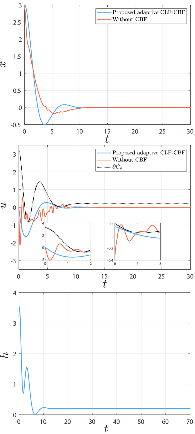
Figure 1: Simulations are performed with proposed adaptive CLF-CBF (blue) and nominal control $v=-x-x^{2}\text{sgn}(u)-u$ (magenta) The black dashed lines indicate the boundary of safety set $\mathcal{U}$.

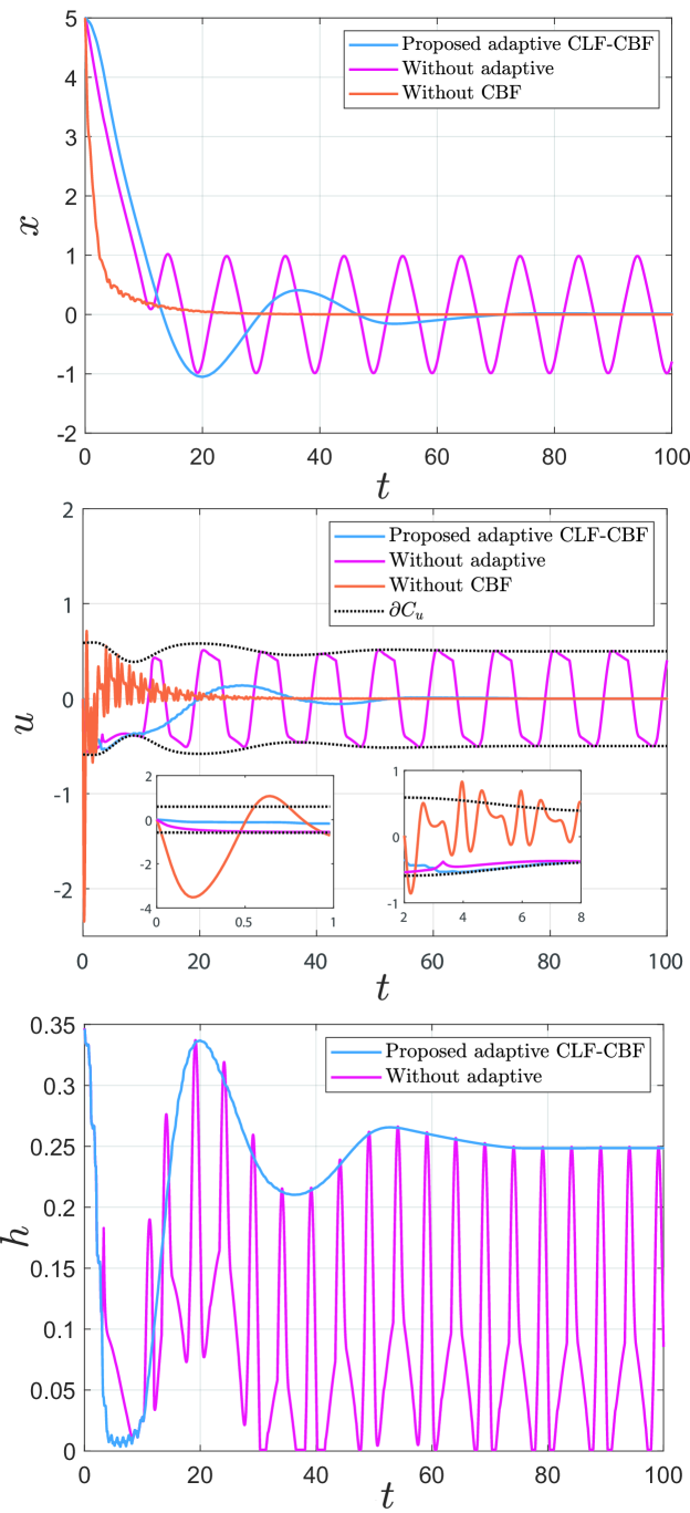
Figure 2: Simulations are performed with proposed adaptive CLF-CBF (blue), nominal control in (31) (orange), and CLF-CBF without adaptive (magenta). The black dashed lines indicate the boundary of safety set $\mathcal{U}$.

We first apply the proposed input constraint CBF-based controller to the system (12). We define the barrier function as $h(x,u)=\kappa-u$ for system (12), where $\kappa(x)=(x-1)^{2}-0.8$. Using system transformation in Section IV-A, the auxiliary control input $v$ for system (12) follows $\dot{u}=v$. Our goal is to design the auxiliary control input $v$, such that $\lim_{t\to\infty}x(t)\to 0$ with $u\in\mathcal{C}_{u}$ for all $t\geq 0$ in system (12). To achieve this objective, one can design a nominal controller $\phi$ as $\phi=-x-x^{2}\text{sgn}(u)-u$. We set the initial conditions as $x(0)=3$ and $u(0)=0$, and set the constraint as $\kappa=(x-1)^{2}-0.8$ with a enough large constant $\Pi_{\kappa}=15$ to satisfied $\lVert\dot{\kappa}\rVert\leq\Pi_{\kappa}$. The proposed controller (blue) is compared to a normal CLF-CBF controller (magenta), which proposed in [22] and not consider the adaptive control for uncertainty. The corresponding simulation results are shown in Figure 2. We can see the system (12) reaches the input constraint around $t=1.5,6.0$, and $7.0$ seconds, where nominal control input leaves the safe set. The proposed method remains feasible and safe for the entire duration, by applying brakes early, around $t=6.5$ seconds, instead of $t=6.0$ seconds.

In the second numerical study, we consider a planar single-integrator uncertain system by letting $f(x)=0$, $g(x)=1$ in (IV-A). We set the time-varying disturbances as

$$d_{x}(t)=d_{u}(t)=\begin{cases}\frac{d_{\max}}{2}t,\quad 0\leq t<\frac{T}{6},\\ d_{\max}t,\quad\frac{T}{6}\leq t<\frac{T}{3},\\ \frac{d_{\max}}{2}(\frac{T}{2}-t),\quad\frac{T}{3}\leq t<\frac{2T}{3},\\ -d_{\max},\quad\frac{2T}{3}\leq t<\frac{5T}{6},\\ \frac{d_{\max}}{2}(t-T),\quad\frac{5T}{6}\leq t\leq T,\end{cases}$$ (70)

and the maximum amplitude of the disturbance $d_{\max}=1$. We set the system initial conditions as $x(0)=5,u(0)=0$. The positive constants in the simulation are selected as $c_{x}=c_{u}=0.21$, $\theta_{x}=\theta_{u}=0.1$, $\varrho=0.95$ and $\Pi_{\kappa}=15$. Other parameters in this simulation are selected as $\nu=0.1$, $l=5$, $\bar{d}_{i}=20$, $T=120$s and $\lambda_{x}=\lambda_{u}=1$.

We intend to control the system to an equilibrium point $\lim_{t\to\infty}x(t)=0$ with a state and time-related barrier function which follows the definition in (11) and (18), and we further define $\kappa=\left(-0.1\sin(x)-1/(t+10)+0.25\right)^{\frac{1}{2}}$. Then our proposed controller (blue) for system (30) is adopted by solving the QP problem (68), (69) where the adaptive weight $\hat{w}_{h,j}$, $\hat{w}_{x,i}$ and $\hat{w}_{u,i}$ are updated by (54) and (2). We compared the proposed controller with the normal CLF-CBF controller (magenta) proposed in [22], and only using the nominal controller in (31) without using CBF (orange). The simulation results are shown in Figure 2. The system approaches the input constraint from $t=2.0$ to $8.0$ seconds, where nominal control input leaves the safe set. Both the proposed method and the CLF-CBF (without adaptive) method remain feasible and safe for the entire duration, by applying brakes early, from $t=3.0$ to $8.0$ seconds. However, without adaptive laws, the CLF-CBF method fails to force the system to the equilibrium, while the proposed adaptive CLF-CBF method is able to converge the system trajectory and keep the input-constrained system safe.

VI Conclusion

The adaptive input-constrained CBF scheme in this paper effectively addresses the challenges of controlling full-state and input-constrained nonlinear systems. By employing an input-to-output auxiliary transformation, the original input constraints are converted into an output CBF design, thus bypassing the limitations imposed by the constraints. An adaptive approach manages time-varying input constraints with a specially designed update law. Simulation results validate the algorithm’s effectiveness. Future research could explore nonsmooth CBF input-constraint issues, and refine the algorithm for specific applications in real-world scenarios.

References

- [1] Teodor Tomić, Christian Ott, and Sami Haddadin. External wrench estimation, collision detection, and reflex reaction for flying robots. IEEE Transactions on Robotics, 33(6):1467–1482, 2017.
- [2] Lampros N Bikas and George A Rovithakis. Prescribed performance under input saturation for uncertain strict-feedback systems: A switching control approach. Automatica, 165:111663, 2024.
- [3] Mario Zanon and Sébastien Gros. Safe reinforcement learning using robust mpc. IEEE Transactions on Automatic Control, 66(8):3638–3652, 2020.
- [4] Raffaele Soloperto, Johannes Köhler, and Frank Allgöwer. A nonlinear mpc scheme for output tracking without terminal ingredients. IEEE Transactions on Automatic Control, 68(4):2368–2375, 2022.
- [5] Hans Joachim Ferreau, Hans Georg Bock, and Moritz Diehl. An online active set strategy to overcome the limitations of explicit mpc. International Journal of Robust and Nonlinear Control: IFAC-Affiliated Journal, 18(8):816–830, 2008.
- [6] Emanuele Garone and Marco M Nicotra. Explicit reference governor for constrained nonlinear systems. IEEE Transactions on Automatic Control, 61(5):1379–1384, 2015.
- [7] Yudan Liu, Joycer Osorio, and Hamid Ossareh. Decoupled reference governors for multi-input multi-output systems. In 2018 ieee conference on decision and control (cdc), pages 1839–1846. IEEE, 2018.
- [8] Yuan-Xin Li. Barrier lyapunov function-based adaptive asymptotic tracking of nonlinear systems with unknown virtual control coefficients. Automatica, 121:109181, 2020.
- [9] Alireza Mousavi, Amir HD Markazi, and Antonella Ferrara. A barrier function-based second order sliding mode control with optimal reaching for full state and input constrained nonlinear systems. IEEE Transactions on Automatic Control, 2023.
- [10] Ye Cao, Yongduan Song, and Changyun Wen. Practical tracking control of perturbed uncertain nonaffine systems with full state constraints. Automatica, 110:108608, 2019.
- [11] Dapeng Li, Hong-Gui Han, and Jun-Fei Qiao. Composite boundary structure-based tracking control for nonlinear state-dependent constrained systems. IEEE Transactions on Automatic Control, 2024.
- [12] Chenguang Yang, Dianye Huang, Wei He, and Long Cheng. Neural control of robot manipulators with trajectory tracking constraints and input saturation. IEEE Transactions on Neural Networks and Learning Systems, 32(9):4231–4242, 2020.
- [13] Xu Jin. Adaptive fixed-time control for mimo nonlinear systems with asymmetric output constraints using universal barrier functions. IEEE Transactions on Automatic Control, 64(7):3046–3053, 2018.
- [14] Aaron D Ames, Xiangru Xu, Jessy W Grizzle, and Paulo Tabuada. Control barrier function based quadratic programs for safety critical systems. IEEE Transactions on Automatic Control, 62(8):3861–3876, 2016.
- [15] Xiangru Xu. Constrained control of input–output linearizable systems using control sharing barrier functions. Automatica, 87:195–201, 2018.
- [16] Aaron D Ames, Gennaro Notomista, Yorai Wardi, and Magnus Egerstedt. Integral control barrier functions for dynamically defined control laws. IEEE control systems letters, 5(3):887–892, 2020.
- [17] Wenceslao Shaw Cortez and Dimos V Dimarogonas. Safe-by-design control for euler–lagrange systems. Automatica, 146:110620, 2022.
- [18] Junjie Fu, Guanghui Wen, and Xinghuo Yu. Safe consensus tracking with guaranteed full state and input constraints: A control barrier function based approach. IEEE Transactions on Automatic Control, 2023.
- [19] Devansh R Agrawal and Dimitra Panagou. Safe control synthesis via input constrained control barrier functions. In 2021 60th IEEE Conference on Decision and Control (CDC), pages 6113–6118. IEEE, 2021.
- [20] Wenceslao Shaw Cortez, Xiao Tan, and Dimos V Dimarogonas. A robust, multiple control barrier function framework for input constrained systems. IEEE Control Systems Letters, 6:1742–1747, 2021.
- [21] Gennaro Notomista and Matteo Saveriano. Safety of dynamical systems with multiple non-convex unsafe sets using control barrier functions. IEEE Control Systems Letters, 6:1136–1141, 2021.
- [22] Aaron D Ames, Samuel Coogan, Magnus Egerstedt, Gennaro Notomista, Koushil Sreenath, and Paulo Tabuada. Control barrier functions: Theory and applications. In 2019 18th European control conference (ECC), pages 3420–3431. IEEE, 2019.
- [23] Andrew J Taylor and Aaron D Ames. Adaptive safety with control barrier functions. In 2020 American Control Conference (ACC), pages 1399–1405. IEEE, 2020.
- [24] Antonella Ferrara, Gian Paolo Incremona, and Claudio Vecchio. Adaptive multiple-surface sliding mode control of nonholonomic systems with matched and unmatched uncertainties. IEEE Transactions on Automatic Control, 2023.
- [25] Ali Heydari. Stability analysis of optimal adaptive control using value iteration with approximation errors. IEEE Transactions on Automatic Control, 63(9):3119–3126, 2018.
- [26] Xiucai Huang, Changyun Wen, and Yongduan Song. Adaptive neural control for uncertain constrained pure feedback systems with severe sensor faults: A complexity reduced approach. Automatica, 147:110701, 2023.
- [27] Aaron D Ames, Xiangru Xu, Jessy W Grizzle, and Paulo Tabuada. Control barrier function based quadratic programs for safety critical systems. IEEE Transactions on Automatic Control, 62(8):3861–3876, 2016.