An exhaustive selection of sufficient adjustment sets for causal inference
Abstract
A subvector of predictor that satisfies the ignorability assumption, whose index set is called a sufficient adjustment set, is crucial for conducting reliable causal inference based on observational data. In this paper, we propose a general family of methods to detect all such sets for the first time in the literature, with no parametric assumptions on the outcome models and with flexible parametric and semiparametric assumptions on the predictor within the treatment groups; the latter induces desired sample-level accuracy. We show that the collection of sufficient adjustment sets can uniquely facilitate multiple types of studies in causal inference, including sharpening the estimation of average causal effect and recovering fundamental connections between the outcome and the treatment hidden in the dependence structure of the predictor. These findings are illustrated by simulation studies and a real data example at the end.
Keywords: sufficient adjustment set, ignorability assumption, dual inverse regression, gaussian copula, collider
1 Introduction
Causal inference commonly refers to estimating the causal effect of a treatment variable on an outcome variable of interest from observational studies. Usually, the treatment variable is binary, under which the potential outcome framework (Rubin, 1974) is a popular tool in the literature to formulate the causal inference theory. The potential outcomes, denoted by and , are the outcome variables if a subject hypothetically receives the treatment (with ) and does not receive the treatment (), respectively. The average causal effect is then defined as , and, given a predictor that measures the subject’s characteristics, the conditional average causal effect is defined as . Because each individual falls into exactly one treatment group in reality, i.e. indexed by , both and are observable only in the corresponding treatment group. To address their missing, two assumptions are commonly adopted in the literature: first, the ignorability assumption
| (1) |
which states that the treatment is randomly assigned regardless of or given (Rosenbaum and Rubin, 1983), second, the common support condition
| (2) |
which avoids extrapolation when using each treatment group to model the entire population (Rosenbaum and Rubin, 1983). Here, denotes the support of a distribution. Under (1) and (2), is identical to for each . Since the latter are estimable by the observed sample, as are the aforementioned causal effects.
To secure the ignorability assumption (1), researchers often collect a large-dimensional that includes all the confounders affecting both and . This however hinders interpretation and more importantly triggers the “curse-of-dimensionality” in fitting , generating unreliable causal effect estimation. Consequently, causal inference can be facilitated if one finds a subvector of , denoted by where , that satisfies
| (3) |
for or . Suppose satisfies (3) for and satisfies (3) for . The average causal effect can then be rewritten as
| (4) |
and can be estimated accurately if both and have small cardinalities. Following Guo et al. (2022), we call any that satisfies (3) for or a sufficient adjustment set. Denote the collection of such sets for the corresponding by . Due to the potential complexity of causal effect, can differ freely from , so it is suitable to discuss them separately. Hereafter, we refer to as each of and if no ambiguity is caused.
In the literature, special elements of have been widely studied rooted in the sparsity assumption on the treatment model and/or the outcome model for . For example, Weitzen et al. (2004) assumed sparsity on , that is,
| (5) |
under which satisfies (3) and thus is a sufficient adjustment set. Similarly, Shortreed and Ertefaie (2017) and Tang et al. (2023) assumed the sparsity of in terms of
| (6) |
where is also a sufficient adjustment set satisfying (3). Under both (5) and (6), VanderWeele and Shpitser (2011) studied another sufficient adjustment set , and De Luna et al. (2011) considered two special locally minimal sufficient adjustment sets starting with variable selection on (5) and (6), respectively, where the local minimality of means that no proper subset of satisfies (3). There are generally non-unique and even numerous locally minimal sets in ; see the directed acyclic graph in Figure 1 where , , and are such sets with only the first two detectable by De Luna et al.’s approach. We refer to Guo et al. (2022) for other related works that rely on prior knowledge about the causal graph.
As pointed out in Witte and Didelez (2019) and Henckel et al. (2022), the optimal sufficient adjustment set varies with the specific causal effect of interest. For example, the formula (4) suggests that the locally minimal sets are best among all in to estimate the average causal effect. A thorough investigation to this end however requires estimating all the locally minimal sets in , which, as seen above, remains unavailable in the literature. Besides causal effect estimation, often the purpose of causal inference is to understand the fundamental connection between and revealed by the subject’s personal characteristics , which hinges on the dependence within and cannot be detected by (5) and (6) that only model and . These together urge the need of exhaustively recovering and in order to facilitate the widest subsequent causal inference, which we will study in this paper for the first time in the literature. The details of how to use and , particularly in uncovering the deep dependence mechanism between and , will be elaborated in §5 later.
Because (3) involves two responses and we only focus on their connection via , it differs from and is more complex than the conventional variable selection that only involves one response, e.g. (6). First, it does not require the sparsity assumption (5) or (6). For example, suppose affects and through some non-sparse and , respectively, and ; then both (5) and (6) fail but is marginally independent of . For the most generality of the proposed work, we do not assume (5) or (6) (except in §), despite that they are common adopted in the literature as mentioned above. Second, while any superset of in (6) also satisfies (6), this can fail for (3); see Figure 1 again where satisfies (3) but does not. Similarly, while any and that satisfy (6) implies that also satisfies (6), this nesting property generally fails for (3), leading to the aforementioned non-uniqueness of the locally minimal sets in . Therefore, to recover and in general, one must evaluate the validity of (3) exhaustively for all , and any smoothing procedure that mimics the lasso method (Tibshirani, 1996) can be inefficient due to the presence of multiple minima. Simplification in some special cases will be discussed in §5.
The evaluation of (3) requires a quantitative criterion that has negligible values if and only if . Because can be large-dimensional when is close to , certain modeling assumptions are necessary to avoid the “curse-of-dimensionality” for the corresponding criteria. To this end, we modify the dual inverse regression methods recently proposed by Luo (2022), which conducts dimension reduction concerning (3) with replaced by a general response and with replaced by a free low-dimensional linear combination . To address the missing of and the dimensionality of , we start with assuming normality on with possibly heterogeneous covariance matrix, and then generalize it to a semiparametric Gaussian copula that allows skewness and heavy tails, etc. The proposed criteria are always model-free on and meanwhile accurate in the sample level, given which we use the ridge ratio method, (see, e.g., a relevant reference Xia et al. (2015)), to detect as an illustration among many other choices.
To summarize, the proposed methods innovatively recover the collections of all the sufficient adjustment sets without assuming sparsity on or . They are always model-free on , and meanwhile accurate and easily implementable by adopting flexible parametric or semiparametric model on . The collections of the sufficient adjustment sets facilitate multiple types of causal inference, including sharpening the causal effect estimation and discovering fundamental dependence mechanism between and . In the following, we will first focus on the estimation of ’s and then discuss how to use them for subsequent causal inference. The theoretical proofs are deferred to the Appendix. For simplicity, we assume to be numerical with zero mean throughout the article.
2 A brief review of dual inverse regression
We first review the dual inverse regression methods (Luo, 2022) that inspire the proposed method. Let be a general, presumably fully observed, response in place of . Luo (2022) assumed and estimated a low-dimensional linear combination that satisfies
| (7) |
This coincides with (3) if is replaced with and is restricted to be some . To tackle (7), Luo (2022) employed the candidate matrices in the inverse regression methods (Li, 1991; Cook and Weisberg, 1991; Li and Wang, 2007) as the basic elements, which were originally designed for the conventional sufficient dimension reduction with respect to an individual response. Therefore, to explain the dual inverse regression methods, we first briefly review sufficient dimension reduction and the associated inverse regression methods. As seen later, this is also the key to the proposed methods for relaxing the sparsity assumptions (5) and (6).
Using as the response, sufficient dimension reduction assumes the existence of a low-dimensional such that
| (8) |
For identifiability, Cook (1998) introduced the central subspace as the parameter of interest, defined as the unique subspace of with minimal dimension whose arbitrary basis matrix satisfies (8). To estimate , the aforementioned inverse regression methods commonly use the moments of to construct a matrix-valued parameter, called the candidate matrix and denoted by , whose column space coincides with under mild conditions. For example, the candidate matrices for the sliced inverse regression (Li, 1991) and the sliced average variance estimator (Cook and Weisberg, 1991) are, respectively,
where denotes the covariance matrix of , denotes for any matrices , and coincides with if is discrete and otherwise slices as whenever falls between its th and th sample quantiles, being prefixed. Using induces a -consistent estimator based on the marginal and slice sample moments of (Li, 1991; Cook and Weisberg, 1991), and its theoretical guarantee is that and share the same central subspace as long as the slicing is fine enough (Zhu and Ng, 1995; Li and Zhu, 2007; Li, 2018).
To ensure , the sliced inverse regression requires the linearity condition on or , that is, with and being the mean and the covariance matrix of , and and likewise being the projection matrices,
| (9) |
Besides (9), the sliced average variance estimator and other inverse regression methods require the constant variance condition on either or , as formulated by
| (10) |
When is large and is low-dimensional, both (9) and (10) hold approximately (Diaconis and Freedman, 1984; Hall and Li, 1993). Otherwise, they require or to have a multivariate normal distribution, considering the freedom of unknown . Depending on whether symmetric effect may exist in , etc., researchers can choose the working inverse regression methods in a data-driven manner; see Li (2018) for details. For simplicity, throughout the article we assume that the working always spans the central subspace, subject to (9) and (10).
Let and be the candidate matrices applied to and , respectively, induced from potentially different inverse regression methods. Luo (2022) chracterized (7) by
| (11) |
A dual inverse regression method then solves (11) with , , and replaced by their estimators. To ensure the coincidence between the solutions to (11) and the reduced predictors for (7), Luo (2022) adopted a regularity assumption that equates (7) with
| (12) |
where spans . Similarly to (9) and (10), they also regulated such that (12) is equivalent to for any that solves (11), which again holds approximately if is large and is low-dimensional, and otherwise requires to be normally distributed. We will elaborate variations of these assumptions with the missing of carefully addressed and without the dimension reduction assumption (7).
As pointed out in Luo (2022), the dual inverse regression methods do not rely on the sufficient dimension reduction assumption (8), as a candidate matrix can be implemented even if the corresponding central subspace is . However, the existence of proper solutions to (11) requires one of and to have reduced row rank, which means that either or must be a proper subspace of . This implicit assumption is inherited from the aforementioned regularity assumption related to (12), and it persists in the proposed methods; see detail in §3 later.
3 The proposed method
We first introduce some notations. Let be the collection of all the subsets of , which includes both and as sub-collections. For any , let be the subvector of indexed by , and let be the rest of ; let , , and be the covariance matrix of , that of , and that between and , respectively. For a candidate matrix , let be its submatrix consisting of rows indexed by , and let be the rest of . We use to denote the submatrix of consisting of its columns indexed by , where is omitted from the subscript. Denote the empty set by .
Recall from §1 that the key to selecting the sufficient adjustment sets is to construct a good criterion for (3). This naturally motivates us to extend the dual inverse regression methods. To this end, we echo Luo (2022) to regulate and as follows.
Assumption 1
If , then there must exist some with finite such that is not degenerate at zero.
The generality of Assumption 1 resembles the relative discussion in Luo (2022). An exception is that when both and are , Assumption 1 would imply the failure of (3) for any proper subset of , following . In this case, the validity of Assumption 1 depends on whether we still assume the existence of a proper sufficient adjustment set. Because any model that satisfies the latter must be subtle in this case, and a proper central subspace is commonly accepted along with the wide applicability of sufficient dimension reduction, which particularly allows non-sparse effects of , we assume that at least one of and is a proper subspace of . This sufficient dimension reduction assumption is omitted from the rest of the article, as it is implied implicitly by Assumption 1.
As mentioned in §1, we must address the missing of indexed by , which is briefly mentioned but not carefully dealt with in Luo (2022) due to the use of general response . Under the ignorability assumption (1) and the common support condition (2), coincides with (Luo et al., 2017); the latter, as defined on the sub-population , is readily estimable. Thus, we instead recover by inverse regression, e.g. with
for the sliced inverse regression, where denotes the covariance matrix of . The modified candidate matrix is still denoted by , if no ambiguity is caused. For to span and thus also , and for the same as in §2 to span , we guarantee the linearity condition (9) and the constant variance condition (10) on by adopting
Assumption 2
For , follows a multivariate normal distribution.
By the Bayes Theorem, Assumption 2 implies a parametric model on , which will reduce to the logistic regression if we restrict . The reason that we impose strict normality on rather than using the approximation results mentioned in §2 is that, first, we allow and to be large or even to incorporate complex structures in and (in terms of free ), second, as seen later, a normal induces simple criterion for (3), where can be large-dimensional. Relaxation of Assumption 2 will be proposed in §4.
Because is marginally non-normal under Assumption 2, (11) no longer characterizes (3) if we simply replace with . Instead, we characterize (3) by
| (13) |
This is based on an equivalence property that, under the common support condition (2),
| (14) |
Namely, the former in (14) is on the sub-population indexed by and is what (13) actually characterizes under Assumption 2, as (11) characterizes (12) under normal ; the latter is on the entire population and coincides with (3) under the regularity conditions, as (12) coincides with (7). The key to (14) is the definition of spanned by ; see detail in the Appendix.
Theorem 1
By Theorem 1, (13) can induce good criteria for detecting the sufficient adjustment sets subject to the normality of . As an illustration, we introduce with, if is nonempty,
| (15) |
and with , where denotes the spectral norm. The solution set of , which also minimizes , identifies . For , either or must have reduced row rank, which complies with the assumption above that either or is a proper subspace of . Nonetheless, these matrices can still be non-sparse, indicating the non-sparsity of and mentioned in §1. Again, this generality is not permitted in the existing approaches, even though they only detect special members of (Shortreed and Ertefaie, 2017; Tang et al., 2023).
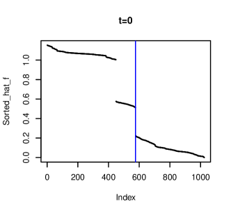
Let be the sample covariance matrix of for , and let and be the consistent estimators of and reviewed in §2. We approximate by plugging these matrix estimates into (15). Based on the resulting , we choose the ridge ratio method (Xia et al., 2015) to detect for simplicity. Let be an rearrangement of such that for each . For large samples, ’s convey a scree plot with mostly indexing its tail; see Figure 2 generated from Model 2 in §6 with and consisting of sets. Define the ridge ratio as
| (16) |
where , and . The use of is to incorporate the extreme case that is constantly zero, which occurs if (3) holds for all . We use the minimizer of , denoted by , to distinguish the tail of the scree plot above, namely
| (17) |
The consistency of follows from that of , , and , subject to appropriate .
Theorem 2
In the numerical studies later, we set and uniformly. When is large, we instead suggest using the sample splitting technique (Zou et al., 2020) to address the growing accumulative noise in , details omitted. The asymptotic study under the high-dimensional settings is deferred to the Appendix.
One issue in implementing is its computational cost for the exhaustive search over , which grows in an exponential rate of . For example, with and the sliced inverse regression used for both and , it takes second on a standard desktop when is but elevates to minutes when grows to . As mentioned in §1, this is generally inevitable due to the complexity of . Simplification in certain cases will be discussed in §5.
4 Extension to non-normal
We now relax Assumption 2 to allow more general semiparametric models for . The key to our extension is the invariance of (3) under any component-wise monotone transformation , denoted by ; that is, for any , (3) holds if and only if
Consequently, we allow to have free component-wise distributions and only require its conditional normality on subject to the corresponding component-wise transformations. This equivalently means a homogeneous semiparametric Gaussian copula model for , that is,
Assumption 3
There exist (completely unknown) monotone mappings such that has a multivariate normal distribution for both .
When , this reduces to the normality of . The applicability of Gaussian copula in fitting skewed or heavily-tailed distributions has been widely recognized (Liu et al., 2012).
Let and be the same matrices as before with replaced by , and let be the covariance matrix of . We generalize in (15) to
| (18) |
if is nonempty, and to . Again, we adopt the ignorability assumption (1), the common support condition (2), and Assumption 1 on . The former two are invariant under the transformation ; the latter requires or to be a proper subspace of , which we assume implicitly. The identification of as the solution set of follows similarly to Theorem 1.
To estimate , we approximate each in two steps. First, within each treatment group , we follow the literature (Klaassen and Wellner, 1997) to use the normal-score estimator to approximate up to a linear transformation specified for ; that is, let , where is the cumulative distribution function of the standard normal distribution, and is the empirical cumulative distribution function for given multiplied by , being the number of observations with . Second, as and differ by a linear transformation asymptotically, we pool them by transforming to , where minimizes the truncated squared loss
| (19) |
over , being the sample mean and being the indicator function. Under the common support condition (2), the truncation in (19) still preserves a certain proportion of the observed sample in the estimation. We take as the pooled estimate of , which permits using the same estimators as before for , , and . The resulting again delivers a consistent by (16) and (17).
5 Facilitation of subsequent causal inference
We now explore how a consistent estimate of can facilitate causal inference. In addition to estimating the average causal effect discussed below (4) in §1, we focus on gaining insights into the dependence mechanism of by studying their directed acyclic graph from . To link the two concepts rigorously, we adopt the Markov condition and the faithfulness assumption (Spirtes, 2010, §2.1) throughout this section, which equate (3) with the -separation of and given in the directed acyclic graph. The faithfulness assumption also excludes the extreme case mentioned in §1, so that one of the active sets for and , denoted by and , respectively, must be a proper subset of . For ease of presentation, we assume known throughout this section, and we leave the review of the directed acyclic graph and the related concepts (e.g. path, fork, descendant, and -separation), as well as the details about its examples used in this section, to the Appendix.
Recall from §1 that, when the average causal effect is of interest, the locally minimal sets are intuitively the optimal choices among all in due to their locally minimal cardinalities. Because these sets may have different cardinalities, e.g. if we replace and in Figure 1 with some larger and , it is necessary to know all the locally minimal sets in to find the optimal choice for the subsequent nonparametric estimation of the average causal effect. This illustrates the gain of knowing in addressing the dimensionality issue for the causal effect estimation without parametric modeling.
In regard of understanding the dependence mechanism between and , also provides unique information beyond the existing literature reviewed in §1. First, as illustrated in Figure 1, some sets in (e.g. ) can index variables of that only have indirect effects on and through the rest of . These variables cannot be detected by the existing methods that model and , but they are potentially the fundamental cause that connects and and thus may attract the researchers’ interest. To explore more from , we next study the bond between the locally minimal sets in and , i.e. that formed by the variables of who directly affect both and . The key is the definition of -separation and that, under the Markov condition and the faithfulness assumption, exactly indexes the forks between and in the directed acyclic graph.
Proposition 4
Under the Markov condition and the faithfulness assumption, we have: () is the intersection of all the locally minimal sets in ; () if and only if has the unique minimal set, in which case itself is the minimal set in .
By Proposition 4(), knowing means knowing all the forks between and . See Figure 3(a), 3(c), and 3(d) where the intersection of all the locally minimal sets in is and forms the only fork with and , also Figure 3(b), 3(e), and 3(f) where this intersection is the empty set and no forks exist in the graph. Due to the dependence between the variables of , which may generate other paths between and , alone is generally insufficient for the -separation of and , that is, ; see Figure 3(b) where is the empty set but and are marginally -connected. Proposition 4() clarifies that if and only if has the unique minimal set. In the language of -separation, this holds if and only if every path between and that has no colliders must include some node that forms a fork between and . The definition of a collider can be found in the next paragraph. In practice, this special case may often occur as it allows otherwise complexity of resulted from the freedom of the paths with colliders. In particular, it is more general than the nesting property for mentioned in §1; see Figure 3(a) where has the unique minimal set and the nesting property fails.
From the nesting of the sets in , we can also recover some important structures of the directed acyclic graph of . Namely, we can identify the types of nodes, particularly the aforementioned collider, that some variables of play in the graph. A collider means some who blocks a path between and via some , which is unrelated to both and if only considering that path. Because a collider can meanwhile be a non-collider in some other path between and (see details below) and thus still related to and , it “carries with its unique considerations and challenges” to causal inference (Pearl et al., 2016, §2.3). To ease the presentation, we next abbreviate a path between and to a path, and abbreviate a set of a collider and its descendants to a collider, if no ambiguity is caused. For any and , we use to denote the rest of if is removed. Let be the collection of such that all the supersets of are also included in .
Proposition 5
Under the Markov condition and the faithfulness assumption, we have:
() for , if there exists such that , then is a non-collider in some path; if there exists such that but , then is a non-collider in some path that has at least one collider;
() for any , if there exists such that and for all , then consists of colliders in the same path.
An immediate corollary of Proposition 5() is that any locally minimal set in can only index the variables of that are non-colliders in some paths, which complies with both the interpretation of colliders and the intuition behind the local minimality. This also complements Proposition 4. Let be the union of all in Proposition 5(). Then must index colliders; see Figures 3(a), 3(b), 3(d), and 3(f) where it detects , and Figure 3(e) where it detects and . This detection however can be non-exhaustive; see Figure 3(c) where is a collider but is the empty set. Because the colliders that detects may as well be non-colliders in the other paths, e.g. in Figures 3(b), 3(d), and 3(f), and in Figure 3(e), we can refine by excluding its elements that satisfy Proposition 5(), and consider the rest as the candidate variables that only serve as colliders and thus redundant for any subsequent causal inference. This excludes in Figures 3(b) and 3(f), and excludes in Figure 3(e), but it fails to exclude in Figure 3(d).
Due to the intrinsic limitation of -separation (Spirtes, 2010), cannot completely determine the paths between and in general. For example, is identical in Figures 3(d) and 3(g). Nonetheless, it is still worth to explore more results towards this end besides those proposed above, as they help the researchers understand the fundamental connection between and via simple and semiparametric estimators of rather than subtle parametric modeling (Spirtes, 2010). This requires tremendous work and is deferred to future.
Finally, if the Markov condition and the faithfulness assumption hold and we partially know the directed acyclic graph of , then the results above can be used conversely to simplify the exhaustive searching process proposed in §3 and lighten the computational burden. These include: (a) by Proposition 4(), we only need to look into all the supersets of ; (b) if some is known to be a collider in every path where it is present, that is, it is a common effect of other variables of and is otherwise unrelated to and , then Proposition 5() justifies that any implies ; (c) if some is known to be a non-collider in every path where it is present, which occurs if it is not a common effect of any pairs of other variables of , then Proposition 5() justifies that any implies .
6 Simulation studies
We use the following five simulation examples to evaluate the proposed methods in recovering both and its sub-collection of locally minimal sets, and in detecting colliders in . The R code can be found in https://github.com/jun102653/confounder-selection. To examine the robustness of the proposed methods to Assumptions 2 and 3, respectively, we generate under various distributions including the marginal normality of and a mixture of continuous and discrete components in . For space limit, we set and defer to the Appendix. In the following, denotes the Bernoulli distribution with mean , denotes , and each is fixed as , being the cumulative distribution function of the F distribution with the degrees of freedom . The random errors for and for are generated from .
-
1.
, , ,
, , , . -
2.
, ,
, , , . -
3.
, ,
, , , . -
4.
, ,
, , except for . -
5.
Same as Model but with in generating replaced by .
These models represent a variety of cases from simple to complex patterns and from weak to strong signals. The effect of on is linear in Model 1 and is complex otherwise, and is much weaker in Model 5 than in Model 4. The effect of on conveys a logistic regression in Models 1-3 and is more subtle in Models 4-5. In Models 1-2, is a collider and detectable by . In Model 3, affects and indirectly and induces one of the three locally minimal sets in . Because has a large cardinality in all the models, i.e. , , , , and , respectively, its recovery is nontrivial especially in Model 5 with weak signals.
Considering the symmetry of in Models 4-5, we use the sliced average variance estimator to construct and for these models, and we use the sliced inverse regression uniformly for the other candidate matrices. To measure the similarity between and some , we use
| (20) |
where denotes the cardinality of a collection. Both measures have range with larger values indicating better similarity, and they complement each other as is sensitive to the number of falsely unselected sets in and is sensitive to the number of falsely selected sets not in . We also report the probability that includes all the locally minimal sets. To see whether truly collects the collider set , we use the rule introduced below Proposition 5 to derive based on , and record and , the numbers of truly and falsely selected colliders. The average of these measures among independent runs are recorded in Table 1, where the sample size is set at and sequentially. For convenience, we call the proposed method that assume normal the normality estimator, and call that assume a Gaussian copula on the Gaussian copula estimator, and denote them by “MN” and “GC” in Table 1.
| Model 1 | Model 2 | Model 3 | Model 4 | Model 5 | ||||||
| MN | GC | MN | GC | MN | GC | MN | GC | MN | GC | |
| 92/94 | 92/94 | 91/96 | 91/96 | 100/74 | 100/74 | 23/78 | 100/93 | 23/77 | 96/76 | |
| 92/95 | 92/94 | 90/95 | 89/95 | 94/76 | 96/75 | 24/76 | 100/89 | 23/76 | 92/73 | |
| 80/79 | 81/80 | 75/74 | 77/75 | 100/93 | 100/95 | 10/11 | 100/100 | 10/10 | 96/92 | |
| 45/31 | 46/31 | 53/19 | 53/18 | |||||||
| 47/28 | 46/32 | 54/49 | 55/47 | |||||||
| MN | GC | MN | GC | MN | GC | MN | GC | MN | GC | |
| 96/98 | 96/98 | 95/99 | 95/99 | 100/74 | 100/74 | 26/76 | 100/100 | 26/76 | 100/98 | |
| 96/98 | 96/98 | 93/98 | 94/98 | 99/74 | 100/74 | 28/75 | 100/100 | 26/74 | 100/96 | |
| 88/88 | 89/88 | 84/81 | 87/82 | 100/99 | 100/100 | 13/14 | 100/100 | 13/12 | 100/100 | |
| 76/4 | 75/5 | 77/3 | 79/2 | |||||||
| 75/6 | 75/6 | 75/21 | 76/22 | |||||||
From Table 1, the two methods consistently recover both and in Models 1-3, where their assumptions on are violated in Model 3. The Gaussian copula estimator also consistently recovers and in Model 4, and its performance is only slightly compromised in Model 5 where the signal is weaker. The inconsistency of the normality estimator in Models 4-5 meets the theoretical anticipation, although the large and indicate that it only under-selects and , that is, most elements in the corresponding and are still sufficient adjustment sets. The consistency of the proposed methods in recovering the minimal sets follows that in recovering and , which particularly suggests their capability in capturing the indirect effects of in Model 3. The methods are less accurate in detecting the colliders, but their improved performance when increases to still indicates their asymptotic consistency in this respect. The otherwise performances of the proposed methods are also enhanced when grows from to , except for the normality estimator in Models 4-5.
7 Application
We apply the proposed work to a study of whether the mother smoking during pregnancy causes the infant’s low birth weight (Kramer, 1987). The dataset available at http://www.stata-press.com/data/r13/cattaneo2.dta. was analyzed in Almond et al. (2005), Da Veiga and Wilder (2008), and Lee et al. (2017) using a program evaluation approach and a propensity score matching method, etc.. Following Lee et al. (2017), we restrict the sample to the white and non-Hispanic mothers, which include subjects. The outcome variable is the infant’s birth weight measured in grams, and the predictor includes the indicator of alcohol consumption during pregnancy (), the indicator of a previous dead newborn (), the mother’s age (), the mother’s educational attainment (), the number of prenatal care visits (), the indicator of the newborn being the first baby (), and the indicator for the first prenatal visit in the first trimester (). The ignorability assumption (1) was justified in Lee et al. (2017), and the common support assumption (2) is supported by an omitted exploratory data analysis.
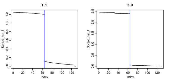
Under the concern of complex , we apply the proposed Gaussian copula estimator with both and from directional regression. As seen in the scree plots of ’s and ’s in Figure 4, both and include the unique minimal set and all of its supersets. This means that the mother’s alcohol consumption during pregnancy satisfies (3) alone for both , and, by Proposition 4, it is the only factor associated with both the mother’s smoking and the infant’s potential birth weights had the mother smoked and had her not smoked.
Using the mother’s alcohol consumption as the univariate predictor, we apply the one-to-one matching method in the R package Matching to estimate the average causal effect. The estimate is grams, with the bootstrap standard deviation equal to grams. This suggests a significant causal effect of the mother’s smoking on the infant’s low birth weight, which is consistent with the findings in the previous studies (Kramer, 1987; Almond et al., 2005; Lee et al., 2017). Applying the same method to the original data with the ambient predictor, the estimate of the average causal effect is similarly grams, but its bootstrap standard deviation is raised to grams, resulting in a less significant conclusion. This illustrates the gain of using small sufficient adjustment sets in sharpening the causal effect estimation.
Acknowledgments and Disclosure of Funding
Wei Luo’s research was supported in part by the National Science Foundation of China (12222117, 12131006). Lixing Zhu’s research was supported in part by the National Science Foundation of China (12131006).
Appendix A Consistency of under the high-dimensional settings
When diverges with , , , and are sequences of matrices with growing dimensions and dynamic entries. Thus, we must regulate the signal strength of the data through these matrices, to preclude weak effects that are infeasible to detect in the sample level. Let denote the minimal nonzero singular value of a matrix, and let be the collection of matrix sequences with and . Without loss of generality, suppose and that span and , respectively, are sequences of semi-orthogonal matrices.
Assumption 4
() ; () There exists such that, for and all the large , .
Part () of this assumption requires that the components of are not ill-correlated, and that each direction in (and likewise in ) has uniformly non-vanishing effect on , both of which are commonly adopted in the relative literature (Zhu et al., 2010; Qian et al., 2019; Tan and Zhu, 2019). Part () of Assumption 4 regulates and to preclude any subtle “local alternative hypothesis” whenever the statements in (14) fail. To incorporate the divergence of , we write in (16) as , which can vary with .
Theorem 6
The lower bound for in Theorem 6 depends on the diverging rate of with respect to as well as the specific inverse regression methods that induce and . For example, when , Wainwright (2019) justified , and Qian et al. (2019) justified that both and are also for the sliced inverse regression, assuming that both and are sparse and have fixed dimensions as diverges; these together imply , that is,
for the consistency of .
Appendix B Review of the directed acyclic graph
We now briefly review the directed acyclic graph commonly used to depict the dependence mechanism of a set of random variables. Each random variable is represented by a node (or called a vertex) in the graph, and their overall dependence is represented by the set of directed edges between the nodes. For example, for any pair of random variables , means that is a cause of and is called an ascendant (or parent) of , and is called a descendant (or child) of . The meaningfulness of these edges requires the local Markov property that there exists a joint distribution of the nodes such that each node is conditionally independent of its non-descendants given its ascendants. Generally, a directed acyclic graph determines the corresponding probabilistic dependence between its nodes, but conversely the probabilistic dependence of a set of variables can only determine the directed acyclic graph up to its equivalence class (Pearl et al., 2016).
A path in the directed acyclic graph is defined as a set of edges such that each node it involves is visited only once. Any path can be decomposed into a set of triplets . The case is called a chain, and it occurs if is a direct cause of and is a direct cause of . The case is called a fork, and it occurs if is a common cause of both and . Both of these mean and thus are indistinguishable by the probablisitc dependence of , The case is called a collider, and it occurs if is a common effect of both and . For ease of presentation, we also call a collider in this case. A path is called blocked by a set of nodes if this set of nodes include at least one of the non-colliders of the path, or if this set of nodes do not include at least one of the colliders (together with its descendants) of the path. A pair of nodes and are called conditionally -separated given a set of nodes if every path between and , i.e. with these two as the ending nodes, is blocked by . Namely, this occurs if and only if both of the following two statements hold:
() for each path between and that has no colliders, includes at least one of its nodes;
() for each path between and that has an non-empty set of colliders , where each element of also represents its deccendants for simplicity, is either not a superset of or includes at least one of the non-colliders in this path.
Under the Markov condition and the faithfulness assumption (Spirtes, 2010, §2.1), the conditional -separation between any and given is equivalent to the probabilistic independence . Thus, the definition of -separation above will be used to provide for the examples of directed acyclic graph and to prove the relative propositions listed in the main text. The former is presented in the rest of this section, and the latter is deferred to Appendix C later. For simplicity, we write any as throughout this section, and use to denote the collection of all the supersets of . The former should not cause ambiguity with the labels of the equations in the main text, which only appear in the other sections of the appendix.
The following causal graph is the example in Section 1 of the main text.
It contains two paths between and : and , where the latter include a collider . Thus, the -separation of and given is equivalent to that indexes at least one variable in the first path and meanwhile either indexes or or does not index in the second path. This means
with the locally minimal sets being , , and . Note that and there is no unique minimal set in in this case, which comply with Proposition 4 of the main text.
The following graph is the example in Figure 3(a) of the main text.
It contains two paths between and : and , the latter including a collider. Thus, the -separation of and given is equivalent to that, first, includes , second, either does not index or indexes at least one of the other nodes in the second path. This means
Hence, has the unique minimal set but does not satisfy the nesting property. Since and , satisfies Proposition 5(), so we have .
The following graph is the example in Figure 3(b) of the main text.
It contains two paths between and : and , the latter including a collider. Thus, the -separation of and given is equivalent to that, first, indexes at least one variable in the first path, second, either does not index or indexes at least one of the other nodes in the second path. This means
Consequently, the intersection of all the local minimal sets in is the empty set, and we have as only satisfies Proposition 5() with and . Because and , also satisfies Proposition 5() and thus is removed from the refined .
The following graph is the example in Figure 3(c) of the main text.
It contains three paths between and : , , and , the latter including a collider. Thus, the -separation of and given is equivalent to that, first, indexes at least one variable in each of the first two paths, second, either does not index or indexes at least one of the other nodes in the last path. This means
Consequently, the intersection of all the locally minimal sets in is , and we have as no elements in , including , satisfy Proposition 5 ().
The following graph is the example in Figure 3(d) of the main text.
It contains four paths between and : , , , , the latter including a collider. Thus, the -separation of and given is equivalent to that, first, indexes at least one variable in each of the first three paths, second, either does not index or indexes at least one of the other nodes in the last path. This means
Consequently, the intersection of all the locally minimal sets in is , and we have as only satisfies Proposition 5() with and . However, as does not satisfy Proposition 5(), it is kept in the refined .
The following graph is the example in Figure 3(e) of the main text.
It contains four paths between and : , , , and , the latter three including colliders. Thus, the -separation of and given is equivalent to that, first, indexes at least one variable in the first path, second, either does not index the collider or indexes at least one of the other nodes in the last three paths. This means
Consequently, the intersection of all the locally minimal sets in is the empty set, and we have as these two elements satisfy Proposition 5() with , , and . As satisfies Proposition 5() with and and does not, only is removed from the refined .
The following graph is the example in Figure 3(f) of the main text.
It contains four paths between and : , , , and , the latter including a collider. Thus, the -separation of and given is equivalent to that, first, indexes at least one variable in each of the first three paths, second, either does not index or indexes at least one of the other nodes in the last path. This means
Consequently, the intersection of all the locally minimal sets in is the empty set, and we have as only satisfies Proposition 5() with and . Since also satisfies Proposition 5() with and , it is removed from the refined .
The following graph is the example in Figure 3(g) of the main text.
It contains four paths between and : , , , , the latter including a collider. Thus, the -separation of and given is equivalent to that, first, indexes at least one variable in each of the first three paths, second, either does not index or indexes at least one of the other nodes in the last path. This means
which is exactly the same as for Figure 3(d).
Appendix C Proof of Theorems and Propositions
We now give the proofs of all the theoretical results in the order they appear in the main text. The proof of Theorem 6 above is placed at the end of this section.
C.1 Proof of the equivalence property (14)
This equivalence property is important for the proof of Theorem 1, so we prove it first. For simplicity, we use to denote the pdf of a continuous random vector. The key to the proof is by the definition of , which means for any . Under the common support condition (2), this means
| (21) |
for any . If , then reduces to , which, by (21), means and consequently
| (22) |
The latter readily implies . Conversely, if , then as is (22). By (21), we have
which means that is invariant of and thus reduces to , and consequently . The latter means . This completes the proof.
C.2 Proof of Theorem 1
For simplicity, we omit the phrase “almost surely” in this proof. Under the ignorability assumption (1), satisfies (3) if and only if, for any with finite ,
| (23) |
This is because is binary and the right-hand side of (23) equals or equivalently under (1). By the definition of and , (23) is equivalent to
which is equivalent to . Under Assumption 1, this is also equivalent to , which, under the common support condition (2) and by (14), is further equivalent to
| (24) |
Under Assumption 2, (24) is equivalent to , which, by simple algebra, can be rewritten as (13). This completes the proof.
C.3 Proof of Theorem 2
By simple algebra, is a -consistent estimator of for . From Section 2, we also have and . These readily imply
| (25) |
Also see the proof of Theorem 6 below for more relative details. Suppose first. Since , (25) implies that, for ,
| (26) |
which means or equivalently
| (27) |
for some with probability converging to one. Thus, it suffices to prove with probability converging to one. Given (27), (26) means
Together with and , we have, uniformly for ,
for and some . Together with , this readily implies with probability converging to one. Now suppose , then the first part of (26) implies . Together with , we have or equivalently with probability converging to one. This completes the proof.
C.4 Proof of Theorem 3
The proof follows the proof of Theorem 2 if we show , , and for , which would be obvious if we replace with the true for . Thus, it suffices to show that the impact of using in place of is in estimating the conditional and marginal moments in , , and . These resemble the asymptotic studies for the normal-score estimator in the Gaussian copula model (Klaassen and Wellner, 1997; Serfling, 2009; Hoff et al., 2014; Mai et al., 2023). For example, the -consistency of can be proved exactly the same as for Theorem of Klaassen and Wellner (1997), and, if we use the sliced inverse regression for and assume that has the standard normal distribution without loss of generality, then, similarly to the proof of Theorem in Klaassen and Wellner (1997), we have
where the last equality is by Donsker’s Theorem. The -consistency of involves the merged estimator and thus is more tedious, but the proof essentially repeats those above as has a simple form and the coefficients therein are derived by the simple minimal truncated squared loss. Thus, we omit the details. This completes the proof.
C.5 Proof of Proposition 4
Proof of () Since indexes the variables of that are uniquely informative to both and , each of which forms a fork between and , must be included in each locally minimal for the conditional -separation of and given . Conversely, if , that is, does not form a fork between and , then the rest of still induces the conditional -separation of and and consequently satisfies (3), which means that there exists with . Thus, the intersection of all must be a subset of . These together imply that is exactly the intersection of all the locally minimal sets in .
Proof of () Suppose includes some . From the proof of () above, there must exist some with , which means . Thus, if there exists the unique minimal set in , this set must be a subset of . Together with () above, this set must further be , which also means . The “only if” part is obvious based on () above. This completes the proof.
C.6 Proof of Proposition 5
The proof is a direct application of the definition of -separation (see Appendix B above).
Proof of ()-part one For , if there exists such that , then there exists a path between and that is blocked by but not blocked by . Thus, this path either does not include any collider, under which it exactly includes among all indexed by , or it includes a set of colliders and its non-colliders exactly include among all indexed by . In both cases, is a non-collider in some path between and .
Proof of ()-part two First, any means includes at least one non-collider in every path between and that has colliders; otherwise, we can add to exactly all the colliders in the path where does not include any non-collider, and the resulting does not block and in that path and thus is not in . Conversely, we have as long as includes at least one non-collider in every path between and ; the proof is easy from the definition of -separation and omitted. Now suppose , , and . Then does not include any non-collider in some path that has colliders, but does include a non-collider in the same path. Thus, must be the non-collider in that path.
Proof of () Continued from the proof of ()-part two above, if and there exists such that and for any , then does not include any non-collider in at least one path that has colliders, includes all the colliders in at least one of these paths, and any must not include all the colliders in any of these paths. These together imply that exactly consists of all the colliders in the same path.
C.7 Proof of Theorem 6
The proof follows the proof of Theorem 2 as long as we can show:
() ;
() if , then ;
() if , then .
Proof of i: for any , we can write as , and likewise write . Since and , under Assumption 4() that , we have . Similarly, we also have . Recall that, for general matrices and their estimators ,
where the first two inequalities are the triangle inequalities for norms. These together imply
Since is a projection matrix under the inner product , we have for all , which means
Likewise, we also have , which together imply . Since , we have
| (28) |
Since for a general matrix and its arbitrary submatrix , we have
uniformly for . Since under Assumption 4(), we also have
and similarly uniformly for , where the first equality is by Weyl’s Theorem. Plugging these into (C.7), we have, uniformly for , , which implies
Together with shown above, this implies ().
Proof of () Write and where both and have full row rank. Since and and are sequences of semi-orthogonal matrices, we have and . Together with Assumption 2 and Assumption 4(), the former again indicating the constant variance condition (10) on , these imply
| (29) |
for some . This readily implies ().
Appendix D Additional simulation results for
We now raise to for the simulation models in Section 6 of the main text, with still set at and sequentially. For clarity, we change to in Model ; the other model settings remain the same. The results based on independent runs are summarized in Table 2. Compared with Table 1 in the main text for , most phenomena can still be observed in Table 2, indicating the overall consistency of the proposed methods as well as their robustness against the dimensionality of . The only notable step-down is that, when , the Gaussian copula estimator only selects of the sufficient adjustment sets in and of those in in Model 5, where the weak signals are again present. In addition, the slightly larger and and the slightly smaller for in Models 1-2 compared with Table 1 suggest that becomes a slightly more conservative choice as grows, that is, it leads to a larger that includes more sets in .
| Model 1 | Model 2 | Model 3 | Model 4 | Model 5 | ||||||
| MN | GC | MN | GC | MN | GC | MN | GC | MN | GC | |
| 94/89 | 94/89 | 90/93 | 89/93 | 100/74 | 100/74 | 17/79 | 87/69 | 16/80 | 52/70 | |
| 94/89 | 93/89 | 89/90 | 88/90 | 92/76 | 94/76 | 16/80 | 82/65 | 16/80 | 39/76 | |
| 91/92 | 91/91 | 86/86 | 85/84 | 100/92 | 100/94 | 6/5 | 87/82 | 5/4 | 52/39 | |
| 34/81 | 33/83 | 49/58 | 47/48 | |||||||
| 33/88 | 32/86 | 46/107 | 46/107 | |||||||
| MN | GC | MN | GC | MN | GC | MN | GC | MN | GC | |
| 99/96 | 99/96 | 99/98 | 99/98 | 100/74 | 100/74 | 21/76 | 100/97 | 21/75 | 100/80 | |
| 99/96 | 99/96 | 98/96 | 98/96 | 100/74 | 100/74 | 22/74 | 100/94 | 22/74 | 98/74 | |
| 97/97 | 97/97 | 95/94 | 96/94 | 100/100 | 100/100 | 8/9 | 100/100 | 8/8 | 100/98 | |
| 74/19 | 73/19 | 83/11 | 84/12 | |||||||
| 74/18 | 74/19 | 80/49 | 80/50 | |||||||
References
- Almond et al. (2005) Douglas Almond, Kenneth Y Chay, and David S Lee. The costs of low birth weight. The Quarterly Journal of Economics, 120(3):1031–1083, 2005.
- Cook (1998) R. D. Cook. Regression Graphics. Wiley, New York, 1998.
- Cook and Weisberg (1991) R Dennis Cook and Sanford Weisberg. Sliced inverse regression for dimension reduction: Comment. Journal of the American Statistical Association, 86(414):328–332, 1991.
- Da Veiga and Wilder (2008) Paula Veloso Da Veiga and Ronald P Wilder. Maternal smoking during pregnancy and birthweight: a propensity score matching approach. Maternal and Child Health Journal, 12:194–203, 2008.
- De Luna et al. (2011) Xavier De Luna, Ingeborg Waernbaum, and Thomas S Richardson. Covariate selection for the nonparametric estimation of an average treatment effect. Biometrika, 98(4):861–875, 2011.
- Diaconis and Freedman (1984) Persi Diaconis and David Freedman. Asymptotics of graphical projection pursuit. The annals of statistics, pages 793–815, 1984.
- Guo et al. (2022) F Richard Guo, Anton Rask Lundborg, and Qingyuan Zhao. Confounder selection: Objectives and approaches. arXiv preprint arXiv:2208.13871, 2022.
- Hall and Li (1993) P. Hall and K.-C. Li. On almost linearity of low dimensional projections from high dimensional data. The Annals of Statistics, 47(5):867–889, 1993.
- Henckel et al. (2022) Leonard Henckel, Emilija Perković, and Marloes H Maathuis. Graphical criteria for efficient total effect estimation via adjustment in causal linear models. Journal of the Royal Statistical Society Series B: Statistical Methodology, 84(2):579–599, 2022.
- Hoff et al. (2014) Peter D. Hoff, Xiaoyue Niu, and Jon A. Wellner. Information bounds for Gaussian copulas. Bernoulli, 20(2):604 – 622, 2014.
- Klaassen and Wellner (1997) Chris A.J. Klaassen and Jon A. Wellner. Efficient estimation in the bivariate normal copula model: normal margins are least favourable. Bernoulli, 3(1):55 – 77, 1997.
- Kramer (1987) Michael S Kramer. Determinants of low birth weight: methodological assessment and meta-analysis. Bulletin of the world health organization, 65(5):663, 1987.
- Lee et al. (2017) Sokbae Lee, Ryo Okui, and Yoon-Jae Whang. Doubly robust uniform confidence band for the conditional average treatment effect function. Journal of Applied Econometrics, 32(7):1207–1225, 2017.
- Li (2018) Bing Li. Sufficient dimension reduction: Methods and applications with R. CRC Press, 2018.
- Li and Wang (2007) Bing Li and Shaoli Wang. On directional regression for dimension reduction. Journal of the American Statistical Association, 102(479):997–1008, 2007.
- Li (1991) Ker-Chau Li. Sliced inverse regression for dimension reduction. Journal of the American Statistical Association, 86(414):316–327, 1991.
- Li and Zhu (2007) Yingxing Li and Li-Xing Zhu. Asymptotics for sliced average variance estimation. Annals of Statistics, pages 41–69, 2007.
- Liu et al. (2012) Han Liu, Fang Han, Ming Yuan, John Lafferty, and Larry Wasserman. High-dimensional semiparametric gaussian copula graphical models. 2012.
- Luo (2022) Wei Luo. On efficient dimension reduction with respect to the interaction between two response variables. Journal of the Royal Statistical Society Series B: Statistical Methodology, 84(2):269–294, 2022.
- Luo et al. (2017) Wei Luo, Yeying Zhu, and Debashis Ghosh. On estimating regression-based causal effects using sufficient dimension reduction. Biometrika, 104(1):51–65, 2017.
- Mai et al. (2023) Qing Mai, Di He, and Hui Zou. Coordinatewise gaussianization: Theories and applications. Journal of the American Statistical Association, 118(544):2329–2343, 2023.
- Pearl et al. (2016) Judea Pearl, Madelyn Glymour, and Nicholas P Jewell. Causal inference in statistics: A primer. John Wiley & Sons, 2016.
- Qian et al. (2019) Wei Qian, Shanshan Ding, and R Dennis Cook. Sparse minimum discrepancy approach to sufficient dimension reduction with simultaneous variable selection in ultrahigh dimension. Journal of the American Statistical Association, 2019.
- Rosenbaum and Rubin (1983) Paul R Rosenbaum and Donald B Rubin. The central role of the propensity score in observational studies for causal effects. Biometrika, 70(1):41–55, 1983.
- Rubin (1974) Donald B Rubin. Estimating causal effects of treatments in randomized and nonrandomized studies. Journal of educational Psychology, 66(5):688, 1974.
- Serfling (2009) Robert J Serfling. Approximation theorems of mathematical statistics. John Wiley & Sons, 2009.
- Shortreed and Ertefaie (2017) Susan M Shortreed and Ashkan Ertefaie. Outcome-adaptive lasso: variable selection for causal inference. Biometrics, 73(4):1111–1122, 2017.
- Spirtes (2010) P. Spirtes. Introduction to causal inference. Journal of Machine Learning Research, 11(5), 2010.
- Tan and Zhu (2019) Falong Tan and Lixing Zhu. Adaptive-to-model checking for regressions with diverging number of predictors. The Annals of Statistics, 47(4):1960–1994, 2019.
- Tang et al. (2023) Dingke Tang, Dehan Kong, Wenliang Pan, and Linbo Wang. Ultra-high dimensional variable selection for doubly robust causal inference. Biometrics, 79(2):903–914, 2023.
- Tibshirani (1996) Robert Tibshirani. Regression shrinkage and selection via the lasso. Journal of the Royal Statistical Society Series B: Statistical Methodology, 58(1):267–288, 1996.
- VanderWeele and Shpitser (2011) Tyler J VanderWeele and Ilya Shpitser. A new criterion for confounder selection. Biometrics, 67(4):1406–1413, 2011.
- Wainwright (2019) Martin J Wainwright. High-dimensional statistics: A non-asymptotic viewpoint, volume 48. Cambridge university press, 2019.
- Weitzen et al. (2004) Sherry Weitzen, Kate L Lapane, Alicia Y Toledano, Anne L Hume, and Vincent Mor. Principles for modeling propensity scores in medical research: a systematic literature review. Pharmacoepidemiology and drug safety, 13(12):841–853, 2004.
- Witte and Didelez (2019) Janine Witte and Vanessa Didelez. Covariate selection strategies for causal inference: Classification and comparison. Biometrical Journal, 61(5):1270–1289, 2019.
- Xia et al. (2015) Qiang Xia, Wangli Xu, and Lixing Zhu. Consistently determining the number of factors in multivariate volatility modelling. Statistica Sinica, pages 1025–1044, 2015.
- Zhu et al. (2010) Li-Ping Zhu, Li-Xing Zhu, and Zheng-Hui Feng. Dimension reduction in regressions through cumulative slicing estimation. Journal of the American Statistical Association, 105(492):1455–1466, 2010.
- Zhu and Ng (1995) Li-Xing Zhu and Kai W Ng. Asymptotics of sliced inverse regression. Statistica Sinica, pages 727–736, 1995.
- Zou et al. (2020) Changliang Zou, Haojie Ren, Xu Guo, and Runze Li. A new procedure for controlling false discovery rate in large-scale t-tests. arXiv preprint arXiv:2002.12548, 2020.