Clustering and Alignment: Understanding the Training Dynamics in Modular Addition

Abstract

Recent studies have revealed that neural networks learn interpretable algorithms for many simple problems. However, little is known about how these algorithms emerge during training. In this article, we study the training dynamics of a simplified transformer with 2-dimensional embeddings on the problem of modular addition. We observe that embedding vectors tend to organize into two types of structures: grids and circles. We study these structures and explain their emergence as a result of two simple tendencies exhibited by pairs of embeddings: clustering and alignment. We propose explicit formulae for these tendencies as interaction forces between different pairs of embeddings. To show that our formulae can fully account for the emergence of these structures, we construct an equivalent particle simulation where we find that identical structures emerge. We use our insights to discuss the role of weight decay and reveal a new mechanism that links regularization and training dynamics. We also release an interactive demo to support our findings: https://modular-addition.vercel.app/.

1 Introduction

Mechanistic interpretability aims at reverse-engineering the inner workings of trained neural networks and explaining their behavior in terms of interpretable algorithms. Recent work in this field was very successful in uncovering the algorithms learned by neural networks on simple problems. Zhong et al. [2023] showed that transformers learn to solve modular addition by forming circular structures in the embedding space and applying one of two simple algorithms: a “Clock” algorithm (resembling the way humans read the clock) and a “Pizza” algorithm (unfamiliar, but interpretable; also encountered in this article). Charton [2024] showed that transformers learn to compute the greatest common divisor by identifying the prime factors of the numeric base from the last digits of each number. Quirke and Barez [2024] uncovered that transformers break down the multi-digit addition task into parallel, digit-specific streams, using different algorithms for various digit positions.

However, it remains an open problem to provide a similarly high degree of interpretability for the training dynamics that lead to the emergence of these algorithms. Currently, the most successful approach to understanding the learning process is by uncovering hidden progress measures that increase abruptly during training [Barak et al., 2022]. For example, by constructing two progress measures for the problem of modular addition, Nanda et al. [2023] find that training of neural networks on modular addition can be split into three phases: memorization, circuit formation, and cleanup. While insightful, such methods provide only a high-level description of the training process, without offering a clear explanation of the underlying optimization dynamics. Baek et al. [2024] model the embedding vectors as a particle system of “repons” to explain the experimentally observed phase transition between generalization and overfitting, but they do not attemt to provide a complete account of the training dynamics.

The importance of understanding the training dynamics of neural networks is twofold. First, it can contribute to our understanding of neural networks, which in turn allows us to build safer and more interpretable models [Doshi-Velez and Kim, 2017, Olah et al., 2020]. Second, by understanding the training process, we can more easily improve it. We believe that understanding the training dynamics can play a crucial role in the design of new optimizers and architectures, leading to models that are more accurate and compute-efficient.

2 Our contribution

In this article, we study the training dynamics of a simplified transformer with 2-dimensional embeddings on the problem of modular addition. Our contributions are the following.

Grids and circles

We show that embedding vectors tend to organize themselves into circular and grid-like structures, as depicted in Figure 1. The emergence of circular and grid-like structures is consistent with the findings of Zhong et al. [2023], Gromov [2023] and Liu et al. [2022]. We show that grids and circles play a key role in the generalization performance of the model. We also show that weight decay plays a crucial role in the emergence of circular structures and in reducing grid imperfections.

Figure 1: Embedding vectors self-organize into grids (left) and circles (right).

Clustering and alignment

We show how grids and circles facilitate accurate classification for the subsequent layers by grouping “pair sums” (outputs of the constant attention). We propose an explanation for the emergence of the grids and circles as a result of two simple phenomena: clustering and alignment. We propose explicit formulae for both phenomena as interaction forces between two different pairs of embeddings.

Particle simulation

To prove that our proposed formulae can fully account for the emergence of grids and circles, we construct a particle simulation where particles correspond to embedding vectors and forces correspond to gradients. Forces are computed using only our proposed formulae for clustering and alignment. In this simulation, we show that the particles self-organize into the same structures as the embeddings in the trained transformer: circles, grids, and imperfect grids.

Weight decay

We contribute to the understanding of weight decay by discussing its role in our particular setup. Traditionally, weight decay was understood as a form of $L_{2}$ regularization [Goodfellow et al., 2016]. More recently, it was shown that weight decay plays a much more important role by changing the training dynamics in a desirable way [Zhang et al., 2018]. We show that these two perspectives are in fact complementary: by regularizing one part of the model, we enable the emergence of desirable training dynamics in another part of the model.

We also release an interactive demo to allow the readers to explore the training dynamics and particle simulations for themselves: https://modular-addition.vercel.app/.

3 Architecture

In this article, we study a simplified single-layer transformer with constant attention. A similar setup has been previously used by Liu et al. [2022], Zhong et al. [2023] and Hassid et al. [2022].

The input to the model consists of two tokens $a$ and $b$ representing the two numbers to be added, where $a,b\in\{0,1,\ldots,N-1\}$. The tokens are embedded into vectors $x_{a}$ and $x_{b}$ using an embedding matrix $E\in\mathbb{R}^{N\times D}$, where $D$ is the embedding dimension. For the scope of this article, we focus on the case when $D=2$ for simplicity and ease of visualization. Then, a constant attention mechanism is applied to the embeddings. This is equivalent to computing the sum of the embedding vectors.

Then we apply a linear layer of size $H$ with weight matrix $W_{h}\in\mathbb{R}^{H\times D}$, bias vector $b_{h}\in\mathbb{R}^{H}$, and ReLU activation. Finally, we apply a linear layer of size $N$ with a weight matrix $W_{o}\in\mathbb{R}^{N\times H}$ and bias vector $b_{o}\in\mathbb{R}^{N}$. The output of the model is the logits of the predicted sum. We don’t use any skip connections or normalization layers.

We can formalize the model as follows:

• Inputs: $a,b\in\{0,1,\ldots,N-1\}$

• Embeddings: $x_{a}=E_{a}$, $x_{b}=E_{b}$

• Constant attention: $x=x_{a}+x_{b}$

• Linear layer: $h=\mathrm{ReLU}(W_{h}x+b_{h})$

• Output layer: $o=W_{o}h+b_{o}$

We train the model in full batch mode using the AdamW optimizer [Loshchilov and Hutter, 2019] with a learning rate of $0.01$ and weight decay between $0$ and $1$. We use the cross-entropy loss. Unless specified, we use $N=17$ and $H=32$. The training set consists of 80% of all $N(N+1)/2$ distinct pairs of numbers, chosen randomly. The validation set consists of the remaining 20%.

Figure 2: Sometimes embedding vectors self-organize into imperfect grids.

Weight decay

Weight decay is a broadly used regularization technique for training state-of-the-art deep networks [Loshchilov and Hutter, 2019, Krogh and Hertz, 1991, Andriushchenko et al., 2023]. Weight decay penalizes large weights and biases by applying an exponential decay to each parameter ($\theta$) at every step of the optimization. The decay rate is proportional to the learning rate ($\lambda$) and the weight decay coefficient ($\gamma$), as shown in the following formula:

$$\theta_{t+1}\leftarrow\theta_{t}-\lambda\gamma\theta_{t}$$ (1)

4 Grids and circles: the key to successful generalization

We observe that in trained models, the embedding vectors tend to be positioned in arithmetic progressions, forming either grids or circles. We visualize two examples of these structures in Figure 1. The validation accuracy is highest when the embeddings form these structures most clearly. Sometimes, however, the embeddings self-organize into imperfect grids, as shown in Figure 2. In such cases, the validation accuracy is lower, but still higher than when the embeddings are not aligned at all. We present more examples of these structures in Appendix C. To explore the emergence of these structures in more detail, we invite the reader to use our interactive visualizations. In Appendix F, we show that the similar structures emerge in higher-dimensional embedding spaces.

To quantify this effect, we devise two simple algorithms: one to detect circles, and another to quantify the number of grid imperfections in non-circular structures. Circle detection works by checking if all embeddings have about the same distance to the origin. Grid imperfections are defined as the number of pairs of embeddings whose vector sum is not very close to the vector sum of another pair of embeddings with the same modular sum. Both algorithms are explained in detail in the Appendix A.

Table 1: Validation accuracy and structures formed by embedding vectors.

	Circles		Non-Circles
Weight Decay	Num	Acc	Num	Acc	Grid Imperfections	Correlation
0.0	0	-	100	18.2	$102.2\pm 6.1$	-0.92 [-0.95, -0.88]
0.3	1	77.4	99	34.8	$72.7\pm 6.6$	-0.90 [-0.93, -0.85]
0.6	12	65.9	88	51.6	$39.6\pm 4.0$	-0.84 [-0.89, -0.77]
1.0	18	60.4	82	46.7	$31.6\pm 4.0$	-0.64 [-0.75, -0.49]

• Explanation: We train 100 random initializations for 2000 epochs for various values of weight decay.
  For each value of weight decay, we report the following: the number of circles and their average validation accuracy, the number of non-circles and their average validation accuracy, the average number of grid imperfections for non-circles, and the correlation between the number of grid imperfections and the validation accuracy of non-circles. For circle detection and grid imperfections, see Appendix A.

We run multiple experiments for various values of weight decay and measure the average validation accuracy of circles and non-circles, as well as the correlation between the validation accuracy and the number of grid imperfections of non-circles. We report 95% confidence intervals for the grid imperfections and correlation coefficients [Olivoto et al., 2018]. Results are presented in Table 1. We find that circles consistently have higher validation accuracy than non-circles. For non-circles, we find that the validation accuracy is highly correlated with the number of quantifiable grid imperfections.

The emergence of circles and their high validation accuracy is consistent with the findings of Zhong et al. [2023] and Gromov [2023] who showed that circular structures play an important role in the successful generalization of modular addition. The emergence of grid-like structures is also consistent with the work of Liu et al. [2022] who study similar linear structures in the problem of modular addition.

5 Co-evolution of embeddings and linear layers

In this section, we will model the training process as the co-evolution of two systems: the embeddings and the subsequent layers. The constant attention mechanism sums the embedding vectors to obtain $x=E_{a}+E_{b}$. The subsequent layers then act as a classifier, trying to classify this value as $c=a+b\ (\mathrm{mod}\ N)$ out of $N$ possible values.

In Figure 3, we visualize the embeddings (left) and the classification function formed by the subsequent layers (right) of a model at the end of training. In the right plot, we also plot the sums of the embedding vectors of all pairs in the training set (for the rest of the article, we will refer to them as simply “pair sums”). Pair sums are colored according to their modular sum. We present more examples in Appendix E. We observe that the grid structure makes the pair sums cluster based on the modular sum, which enables successful classification.

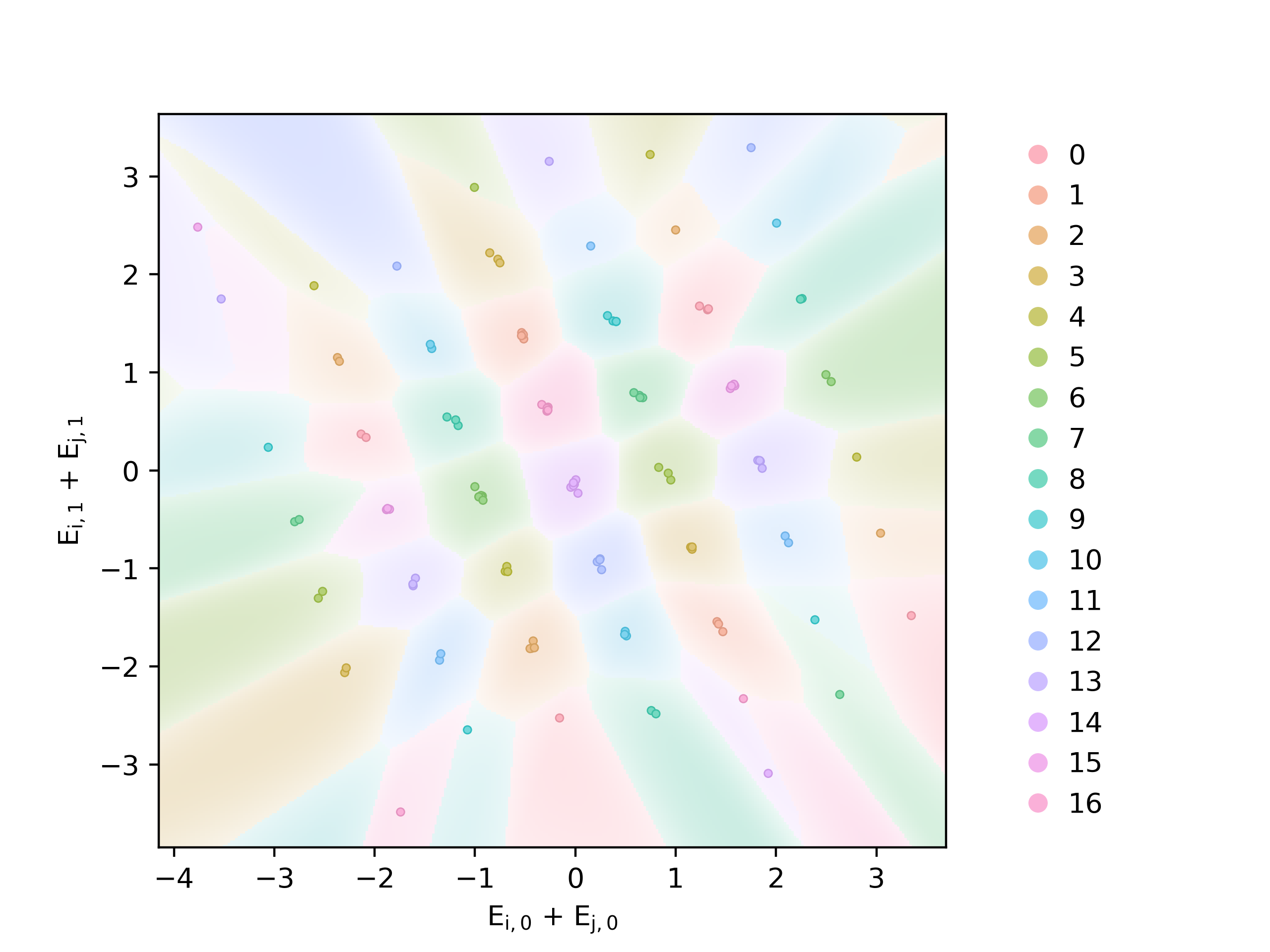
Figure 3: Embedding vectors (left); classifier formed by the subsequent layers
(background, right) and sums of embedding pairs in the training set (markers, right).

In first-order optimization methods, which include the most common optimizers such as SGD and Adam, each parameter is updated according to a gradient that assumes all other parameters are fixed. In practice, this means that each parameter is optimized not only under the constraint of the loss function but also under the constraints of the current state of the other parameters. For our model, this means that the classifier evolves to better classify the pair sums, at the same time that the embeddings evolve to better fit the classifier. We uncover two tendencies that emerge from this dynamic: clustering and alignment.

5.1 Clustering

As depicted in Figure 3, the pair sums tend to cluster based on their modular sum. Let’s try to understand this phenomenon by considering the interaction between two pair sums $x_{ij}=E_{i}+E_{j}$ and $x_{kl}=E_{k}+E_{l}$, where $i,j,k,l\in\{0,1,\ldots,N-1\}$, and $(i,j)$ and $(k,l)$ are two distinct pairs of numbers in the training set.

Let’s first consider the case when $i+j\not\equiv k+l\ (\mathrm{mod}\ N)$. For simplicity, let’s assume that there are no other pair sums in between $x_{ij}$ and $x_{kl}$. In this case, to classify $x_{ij}$ and $x_{kl}$ correctly, the classifier must place a decision boundary between them. This decision boundary will create a gradient that will push $x_{ij}$ and $x_{kl}$ away from each other. Moreover, the closer $x_{ij}$ and $x_{kl}$ are, the narrower the decision boundary will have to be, resulting in a stronger gradient and a stronger push. In other words, the push will be inversely proportional to the distance between the pair sums. We propose the following formula for the gradient at $x_{ij}$ induced by the pair sum $x_{kl}$:

$$g_{ij\leftarrow kl}=g_{r}\cdot\frac{x_{ij}-x_{kl}}{\|x_{ij}-x_{kl}\|}\cdot\frac{1}{\|x_{ij}-x_{kl}\|}$$ (2)

where $g_{r}$ is a repulsion constant. The gradient at $x_{kl}$ is defined analogously: $g_{kl\leftarrow ij}=-g_{ij\leftarrow kl}$.

Now, let’s consider the case when $i+j\equiv k+l\ (\mathrm{mod}\ N)$. Again, for simplicity, let’s assume that there are no other pair sums in between $x_{ij}$ and $x_{kl}$. In this case, $x_{ij}$ and $x_{kl}$ are likely to be inside the same classification region. Both pair sums will be attracted towards the point of maximum classification accuracy, which on average will be the center of the classification region. We will model this case with a constant gradient towards the other pair sum:

$$g_{ij\leftarrow kl}=-g_{a}\cdot\frac{x_{ij}-x_{kl}}{\|x_{ij}-x_{kl}\|}$$ (3)

where $g_{a}$ is an attraction constant. The gradient at $x_{kl}$ is defined analogously: $g_{kl\leftarrow ij}=-g_{ij\leftarrow kl}$. Similar interactions have been previously studied by Baek et al. [2024], Liu et al. [2022], and van Rossem and Saxe [2024].

To understand why we chose to model the attractive force as a constant (rather that, for example, proportional to the distance between the pair sums), consider the following. The softmax classification boundary resembles a sigmoid: the gradient is maximal at the center of the boundary and decreases with distance. Also, a narrower classification boundary has a stronger gradient at its center but an even weaker gradient farther away. Therefore, the strength of the force applied to a particle will depend on two factors: the width of the classification boundary and the distance to the center of the classification boundary. However, neither of those two factors depends on the distance between the two particles. It might seem that the distance between the particles should be correlated to their distance to the classification boundary, but consider that particles could lie slightly outside of the classification boundary, or even in different classification boundaries altogether.

Note that weight decay plays an important role for both attraction and repulsion. Without weight decay, the weights could get arbitrarily large. We explore the impact of weight decay on the magnitude of the weights in Appendix B. This would lead to classification boundries that are very narrow, producing a clustering force that is very strong in a narrow region, but practically non-existent elsewhere. In other words, without weight decay, the classification function would overfit to the pair sums and the evolution of the embeddings would come to a halt.

5.2 Alignment

A different picture emerges when we look at a model where the embeddings form a circle. In Figure 4, we visualize the embedding vectors, pair sums, and the classification function of a model with circular embeddings at the end of training. Pair sums are no longer clustered. Rather, they are aligned along lines that pass through the origin. In this arrangement, the classification regions are skewed and start from the origin, resembling a pizza. This model corresponds exactly to the “pizza” algorithm described by Zhong et al. [2023].

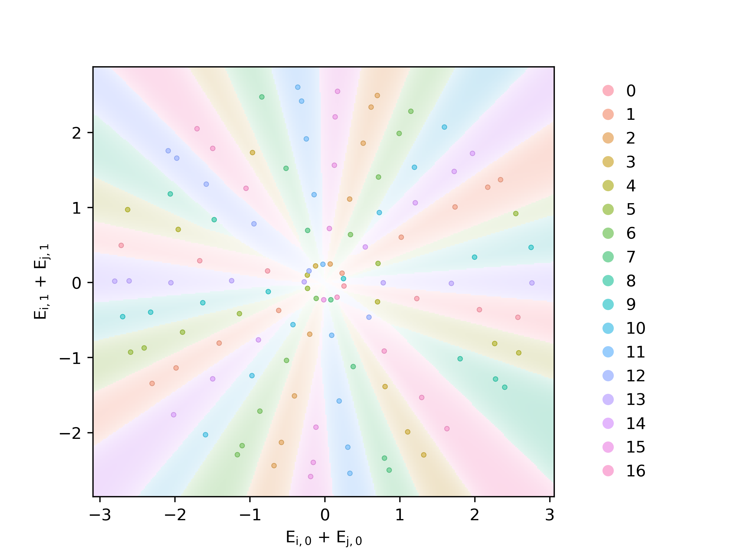
Figure 4: Embedding vectors (left); classifier formed by the subsequent layers
(background, right) and sums of embedding pairs in the training set (markers, right).

In Table 1, we saw that weight decay plays a crucial role in the emergence of circular structures. To understand the mechanism behind the alignment, we need to consider that the classification function is just a sum of ReLU activations of the linear layer.

Weight decay encourages the linear layer to have small weights and biases, which results in linear functions with small slopes and close to the origin. We explore the precise impact of weight decay on the magnitude of the weights and biases in Appendix B. The only aspect that remains completely unconstrained in the direction of the weight vectors. Under these conditions, in order to minimize the training loss, the weight vectors of the linear layer will tend to align with the pair sums. A weight vector aligned with a specific pair sum is maximally useful for the classification layer because it outputs the maximum possible value for that pair sum and the minimum possible value for the other pair sums.

We will model this behavior as follows. For a single pair sum $x_{kl}=E_{k}+E_{l}$, let’s consider a linear function with zero bias ($b=0$) and a weight vector of constant norm that is perfectly aligned with the pair sum ($w=f_{a}\cdot\frac{x_{kl}}{\|x_{kl}\|}$, where $f_{a}$ is a constant). After applying the ReLU activation, the output becomes zero for all points $x$ that oppose the direction of $x_{kl}$ (i.e., $x\cdot x_{kl}<0$). For the other points, the function will have a constant slope of $f_{a}$ in the direction of $x_{kl}$.

Inspired by this simplified model, we propose the following formula for the gradient at $x_{ij}$ produced by the pair sum $x_{kl}$:

$$g_{ij\leftarrow kl}=\begin{cases}0,&\text{if $x_{ij}\cdot x_{kl}\leq 0$}\\ f_{a}\cdot\frac{x_{kl}}{\|x_{kl}\|},&\text{if $x_{ij}\cdot x_{kl}>0$ and }i+j\equiv k+l\ (\mathrm{mod}\ N)\\ -f_{a}\cdot\frac{x_{kl}}{\|x_{kl}\|},&\text{if $x_{ij}\cdot x_{kl}>0$ and }i+j\not\equiv k+l\ (\mathrm{mod}\ N)\\ \end{cases}$$ (4)

6 Particle simulation

In this section, we show that our proposed model can fully account for the emergence of the grids and circles by constructing a particle simulation and showing that particles converge to the same structures as the embedding vectors in the trained transformer.

Figure 5: Particles form circles (left), grids (center), and imperfect grids (right).

We model the training dynamics of the embedding vectors using $N$ particles in a $D$-dimensinal space ($N=17,D=2$). We denote the position of particle $i$ by $x_{i}\in\mathbb{R}^{D}$, $i=1,\ldots,N$. The position $x_{i}$ of particle $i$ corresponds to the embedding vector $E_{i}$ of the number $i$ during training.

We will turn the gradient equations from the previous section into “forces” acting on the $N$ particles. Let $(i,j)$ and $(k,l)$ be two distinct pairs of numbers. We denote the sums of their particle positions as $x_{ij}=x_{i}+x_{j}$ and $x_{kl}=x_{k}+x_{l}$, respectively. The pair $(k,l)$ will induce an equal force on particles $i$ and $j$ (obtained by combining equations 2, 3, and 4):

$$F_{i}=F_{j}=\begin{cases}g_{a}\cdot\frac{x_{kl}-x_{ij}}{\|x_{kl}-x_{ij}\|}&\text{if $x_{ij}\cdot x_{kl}\leq 0$ and $i+j\equiv k+l\ (\mathrm{mod}\ N)$}\\ g_{r}\cdot\frac{x_{ij}-x_{kl}}{\|x_{ij}-x_{kl}\|^{2}}&\text{if $x_{ij}\cdot x_{kl}\leq 0$ and $i+j\not\equiv k+l\ (\mathrm{mod}\ N)$}\\ g_{a}\cdot\frac{x_{kl}-x_{ij}}{\|x_{kl}-x_{ij}\|}+f_{a}\cdot\frac{x_{kl}}{\|x_{kl}\|}&\text{if $x_{ij}\cdot x_{kl}>0$ and $i+j\equiv k+l\ (\mathrm{mod}\ N)$}\\ g_{r}\cdot\frac{x_{ij}-x_{kl}}{\|x_{ij}-x_{kl}\|^{2}}-f_{a}\cdot\frac{x_{kl}}{\|x_{kl}\|}&\text{if $x_{ij}\cdot x_{kl}>0$ and $i+j\not\equiv k+l\ (\mathrm{mod}\ N)$}\\ \end{cases}$$

The force acting on particles $k$ and $l$ is defined analogously. We use $g_{r}=g_{a}=f_{a}=1$. We also weigh the forces so that interactions between pair sums of different modular sum have the same total contribution as those between pair sums of the same modular sum. We initialize the particles randomly according to a normal distribution. At every step of the simulation, we calculate the total force acting on each particle. We then move each particle with a small step in the direction of the total force. We also scale the particle positions to maintain a constant variance and zero mean. We repeat this process for 100 steps. We don’t use any momentum.

We observe that the particles self-organize into the same structures as the embeddings in the trained transformer: circles, grids, and imperfect grids. We visualize a few examples in Figure 5. For more examples, see Appendix D. In Table 2, we present the results of running 100 simulations for various values of $f_{a}$. We find that the relative frequency of circles and the average number of grid imperfections are very similar to the results obtained from the transformer experiments. We also find that increasing $f_{a}$ leads to more circles, which is consistent with our hypothesis that circles emerge as a result of the alignment force.

Table 2: Results of particle simulations for various values of $f_{a}$

$f_{a}$	Number of Circles	Number of Grids	Average Grid Imperfections
0.5	0	100	$35.5\pm 3.7$
1.0	17	83	$36.3\pm 4.8$
2.0	56	44	$42.9\pm 10.1$

7 The role of weight decay

Traditionally, weight decay was understood as a form of $L_{2}$ regularization, improving generalization by constraining the network capacity [Goodfellow et al., 2016]. More recently, a new perspective on weight decay has emerged, suggesting that it plays a much more important role during training by changing the training dynamics in a desirable way [Zhang et al., 2018]. In this section, we combine the two perspectives by discussing the impact of weight decay on the training dynamics in our setup.

In Section 4, we observed that weight decay plays an important role in the successful generalization of the trained model. We propose the following explanation: weight decay changes the training dynamics by strengthening the clustering force and by introducing the alignment force. In turn, these forces facilitate the emergence of grids and circles, which are crucial for the generalization performance of the model. Below we discuss exactly how weight decay impacts clustering and alignment.

In the case of clustering, our proposed clustering force (Equations 2 and 3) is highly dependent on a simplified model of the classification function where the decision boundaries are very wide. Weight decay enables this by limiting the magnitude of the weights of the linear layer and output layer, as we show in Appendix B. Without weight decay, classification boundaries could get arbitrarily narrow, leading to a clustering force that is very strong in a narrow region, but practically non-existent elsewhere. In other words, without weight decay, the classifier would overfit to the pair sums and the embeddings would become stuck in a local minimum.

In the case of alignment, weight decay makes the alignment force (Equation 4) possible by limiting the magnitude of the biases of the linear layer, as we show in Appendix B. This forces the ReLU activations of the linear layer to remain very close to the origin, creating the sort of alignment we have seen. Without weight decay, biases could get arbitrarily large and there would not be any specific point around which the alignment could take place.

This represents a very interesting link between regularization and training dynamics. By regularizing one part of the model, we enable the emergence of desirable training dynamics in another part of the model. Without weight decay, a layer could overfit to the current state of the other layers, limiting them from making further progress. This could explain why weight decay is so effective in training deep learning models [Andriushchenko et al., 2023], which consist of many different layers that need to co-evolve harmoniously during training.

To the best of our knowledge, this link between regularization and training dynamics has not been previously reported. This opens up interesting new questions for future research, such as providing theoretical proof for this phenomenon or showing how it takes place in other problems and architectures.

8 Conclusion

We have explained the training dynamics of a simplified transformer on the problem of modular addition in terms of two simple phenomena: clustering and alignment. We have provided strong evidence for our model using a particle simulation. Our results are very consistent with the previous findings of Zhong et al. [2023] and Gromov [2023], who showed that circular structures play an important role in the successful generalization of modular addition, and Liu et al. [2022], who studied the generalization properties of similar grid-like structures in the problem of modular addition.

We believe that our findings open up many new research directions in the field of mechanistic interpretability by showing that it is possible to provide mechanistic explanations not only for the inner workings of trained neural networks, but also for the emergence of these inner workings during training. Exciting challenges lie ahead in understanding the training dynamics of more complex models and problems.

Limitations

We have focused on a very simplified setting: solving modular addition with a single-layer transformer with constant attention and 2-dimensional embeddings. Significant challenges lie ahead in understanding the training dynamics of more complex models and problems. Morveover, even in this simplified setting, our model lacks a theoretical framework, being supported only by empirical evidence and a qualitative analysis. Providing mathematical proofs for the forces behind the training dynamics is an important direction for future research.

Broder Impact

We believe that understanding the training dynamics of neural networks can play a crucial role in the development of better optimizers and neural architectures that are more interpretable and safer, but also more accurate and compute-efficient. It is important to apply caution and responsible judgment when utilizing these new techniques.

Compute Resources

All experiments were conducted on a cloud instance with a single NVIDIA T4 GPU, 16 GB of RAM, and 16 vCPUs. For the entire study, the instance was running for 271 hours, but we expect that a replication would take less than 24 hours for both the transformer and the particle simulation.

Appendix A Algorithms

A.1 Circle detection

To determine whether the embedding vectors form a circle, we simply consider the ratio of the maximum and minimum distances of the embeddings to the origin. If the ratio is below a certain threshold, we consider the embeddings to form a circle. We use a threshold value of 1.2. For our setup, we observe that this simple algorithm is sufficient to detect circles with great accuracy.

Algorithm 1 Check if Embeddings Form a Circle

1:function is_circle(E: embedding matrix)

2:     $min\_norm\leftarrow\min(\sqrt{x^{2}+y^{2}}\mid(x,y)=E_{i},i\in\{0,\ldots,N-1\})$

3:     $max\_norm\leftarrow\max(\sqrt{x^{2}+y^{2}}\mid(x,y)=E_{i},i\in\{0,\ldots,N-1\})$

4:     return $max\_norm/min\_norm<1.2$

5:end function

A.2 Grid imperfections

We propose a simple measure to quantify the number of grid imperfections inspired by the following fact: in a perfect grid, the vector sums of all pairs of embeddings also form a perfect grid where pair sums are grouped together based on their modular sum.

Our measure works as follows. For each pair of embeddings $(E_{i},E_{j})$, we find the pair of embeddings $(E_{k},E_{l})$ with the closest vector sum. If the modular sum $(i+j)\ \mathrm{mod}\ N$ is different from the modular sum $(k+l)\ \mathrm{mod}\ N$, we consider this pair to be an “imperfection”.

Algorithm 2 Count Grid Imperfections in Embedding

1:function imperfections(E: embedding matrix)

2:     $N\leftarrow\text{len}(embed)$

3:     $pairs\leftarrow\{(i,j)\mid i\in\{0,\ldots,N-1\},j\in\{i,\ldots,N-1\}\}$

4:     $imperfections\leftarrow 0$

5:     for all $(i,j)\in pairs$ do

6:         $min\_dist\leftarrow\infty$

7:         $match\leftarrow\text{False}$

8:         for all $(k,l)\in pairs$ do

9:              if $(i,j)=(k,l)$ then

10:                  continue

11:              end if

12:              $dist\leftarrow\|E_{i}+E_{j}-E_{k}-E_{l}\|$

13:              if $dist<min\_dist$ then

14:                  $min\_dist\leftarrow dist$

15:                  $match\leftarrow i+j\equiv k+l\mod N$

16:              end if

17:         end for

18:         if not $match$ then

19:              $imperfections\leftarrow imperfections+1$

20:         end if

21:     end for

22:     return $imperfections$

23:end function

Appendix B Weight decay and the magnitude of weights and biases

Below we visualize the magnitude of the weights and biases of the linear layer at the end of training for various values of weight decay. We run $10$ random initializations for $2000$ epochs with a learning rate of $0.01$. We plot the average absolute value of the weights and biases of the linear layers among the $10$ runs in Figure 6. We observe that weight decay strongly limits the magnitude of the weights and biases, with biases being limited more than weights.

Figure 6: Average magnitude of the weights and biases of the linear layer at the end of training for various values of weight decay.

Appendix C Embedding vectors

Below we visualize the embedding vectors that emerge from several random initializations in the trained transformer for various values of weight decay, after training for 2000 epochs with a learning rate of 0.01.

in 1.0, 0.6, 0.3, 0.0

C.1 $\mathrm{Weight\ decay}=\w$

in 10,…,29

Appendix D Particle simulation

Below we visualize several particle arrangements that emerge from different random initializations in the particle simulation for various values of $f_{a}$, after running the simulation for 100 steps. We maintain $N=17,D=2,g_{r}=g_{a}=1$.

in 1.0, 2.0, 0.5

D.1 $f_{a}=\f$

in 10,…,29

Appendix E Classifier visualization

Below we visualize the embedding vectors (left) and the classification function formed by the subsequent layers (right) of several models at the end of training. In the right plot, we also plot the sums of the embedding vectors of all pairs in the training set (“pair sums”). Models were trained for 2000 epochs with a learning rate of 0.01 and a weight decay of 0.6.

in 10,…,23

Appendix F Embedding vectors in 3D and 4D

Below we visualize the embedding vectors that emerge from several random initializations in the trained transformer with 3-dimensional and 4-dimensional embeddings. We train for 2000 epochs with a weight decay of 1 and a learning rate of 0.01.

We use three 2D plots to visualize each configuration of embeddings. We project the embeddings onto pairs of dimensions and plot the resulting 2D projections. It is not possible to visualize 3D and 4D embeddings directly, but we can still get a sense of their grid-like or circular structure by examining the 2D projections.

F.1 3-dimensional embeddings

in 0,…,6

F.2 4-dimensional embeddings

in 0,…,7

References

- Andriushchenko et al. [2023] M. Andriushchenko, F. D’Angelo, A. Varre, and N. Flammarion. Why do we need weight decay in modern deep learning? arXiv preprint arXiv:2310.04415, 2023.
- Baek et al. [2024] D. D. Baek, Z. Liu, and M. Tegmark. Geneft: Understanding statics and dynamics of model generalization via effective theory. arXiv preprint arXiv:2402.05916, 2024.
- Barak et al. [2022] B. Barak, B. Edelman, S. Goel, S. Kakade, E. Malach, and C. Zhang. Hidden progress in deep learning: Sgd learns parities near the computational limit. In S. Koyejo, S. Mohamed, A. Agarwal, D. Belgrave, K. Cho, and A. Oh, editors, Advances in Neural Information Processing Systems, volume 35, pages 21750–21764. Curran Associates, Inc., 2022. URL https://proceedings.neurips.cc/paper_files/paper/2022/file/884baf65392170763b27c914087bde01-Paper-Conference.pdf.
- Charton [2024] F. Charton. Learning the greatest common divisor: explaining transformer predictions. 2024.
- Doshi-Velez and Kim [2017] F. Doshi-Velez and B. Kim. Towards a rigorous science of interpretable machine learning. 2017.
- Goodfellow et al. [2016] I. Goodfellow, Y. Bengio, and A. Courville. Deep Learning. MIT Press, 2016. http://www.deeplearningbook.org.
- Gromov [2023] A. Gromov. Grokking modular arithmetic. 2023.
- Hassid et al. [2022] M. Hassid, H. Peng, D. Rotem, J. Kasai, I. Montero, N. A. Smith, and R. Schwartz. How much does attention actually attend? questioning the importance of attention in pretrained transformers. In Y. Goldberg, Z. Kozareva, and Y. Zhang, editors, Findings of the Association for Computational Linguistics: EMNLP 2022, pages 1403–1416, Abu Dhabi, United Arab Emirates, Dec. 2022. Association for Computational Linguistics. doi: 10.18653/v1/2022.findings-emnlp.101. URL https://aclanthology.org/2022.findings-emnlp.101.
- Krogh and Hertz [1991] A. Krogh and J. Hertz. A simple weight decay can improve generalization. Advances in neural information processing systems, 4, 1991.
- Liu et al. [2022] Z. Liu, O. Kitouni, N. S. Nolte, E. Michaud, M. Tegmark, and M. Williams. Towards understanding grokking: An effective theory of representation learning. Advances in Neural Information Processing Systems, 35:34651–34663, 2022.
- Loshchilov and Hutter [2019] I. Loshchilov and F. Hutter. Decoupled weight decay regularization. In International Conference on Learning Representations, 2019. URL https://openreview.net/forum?id=Bkg6RiCqY7.
- Nanda et al. [2023] N. Nanda, L. Chan, T. Lieberum, J. Smith, and J. Steinhardt. Progress measures for grokking via mechanistic interpretability. In The Eleventh International Conference on Learning Representations, 2023. URL https://openreview.net/forum?id=9XFSbDPmdW.
- Olah et al. [2020] C. Olah, N. Cammarata, L. Schubert, G. Goh, M. Petrov, and S. Carter. Zoom in: An introduction to circuits. Distill, 2020. doi: 10.23915/distill.00024.001. https://distill.pub/2020/circuits/zoom-in.
- Olivoto et al. [2018] T. Olivoto, A. D. C. Lúcio, V. Q. de Souza, M. Nardino, M. I. Diel, B. G. Sari, D. K. Krysczun, D. Meira, and C. Meier. Confidence interval width for pearson’s correlation coefficient: A gaussian-independent estimator based on sample size and strength of association. Agronomy Journal, 110(2):503–510, 2018. doi: https://doi.org/10.2134/agronj2017.09.0566. URL https://acsess.onlinelibrary.wiley.com/doi/abs/10.2134/agronj2017.09.0566.
- Quirke and Barez [2024] P. Quirke and F. Barez. Understanding addition in transformers. In The Twelfth International Conference on Learning Representations, 2024. URL https://openreview.net/forum?id=rIx1YXVWZb.
- van Rossem and Saxe [2024] L. van Rossem and A. M. Saxe. When representations align: Universality in representation learning dynamics. arXiv preprint arXiv:2402.09142, 2024.
- Zhang et al. [2018] G. Zhang, C. Wang, B. Xu, and R. Grosse. Three mechanisms of weight decay regularization. arXiv preprint arXiv:1810.12281, 2018.
- Zhong et al. [2023] Z. Zhong, Z. Liu, M. Tegmark, and J. Andreas. The clock and the pizza: Two stories in mechanistic explanation of neural networks. In A. Oh, T. Neumann, A. Globerson, K. Saenko, M. Hardt, and S. Levine, editors, Advances in Neural Information Processing Systems, volume 36, pages 27223–27250. Curran Associates, Inc., 2023. URL https://proceedings.neurips.cc/paper_files/paper/2023/file/56cbfbf49937a0873d451343ddc8c57d-Paper-Conference.pdf.