Stationary Scalar Clouds around Kerr-Newman Black Holes
Abstract
This study investigates scalar clouds around Kerr-Newman black holes within the Einstein-Maxwell-scalar model. Tachyonic instabilities are identified as the driving mechanism for scalar cloud formation. Employing the spectral method, we numerically compute wave functions and parameter space existence domains for both fundamental and excited scalar cloud modes. Our analysis demonstrates that black hole spin imposes an upper limit on the existence of scalar clouds, with excited modes requiring stronger tachyonic instabilities for their formation. These findings lay the groundwork for exploring the nonlinear dynamics and astrophysical implications of scalar clouds.
I Introduction
In the context of electro-vacuum general relativity, the no-hair theorem establishes that all stationary black holes are uniquely defined by their mass, angular momentum and electric charge [1, 2, 3, 4, 5]. This theorem not only addresses the existence of stationary black holes with more degrees of freedom but also describes the dynamical endpoint of gravitational collapse. Testing the no-hair theorem is crucial for understanding black hole physics and can help constrain alternative theories of gravity. For instance, the black-hole spectroscopy program, which analyzes quasinormal modes extracted from gravitational-wave observations, has emerged as a powerful tool for probing the Kerr nature of astrophysical compact objects [6, 7, 8].
While the no-hair theorem dictates that stationary black holes in electro-vacuum spacetime are uniquely described by mass, angular momentum and electric charge, the discovery of the first hairy black hole solution within Einstein-Yang-Mills theory challenged this notion [9, 10, 11]. Since then, numerous counterexamples have emerged [12, 13, 14, 15, 16, 17]. In particular, black holes with scalar hair have attracted great interest, as scalar fields are well-motivated beyond the standard model and can be used to model dark energy and dark matter [18]. However, the existence of asymptotically flat black holes with scalar hair is constrained by the Bekenstein’s uniqueness theorem for -scalar-vacuum [19, 20, 21]. Therefore, such black holes require specific conditions: a non-minimal coupling of the scalar field [22, 23, 24, 25, 26], a violation of spacetime symmetry for the scalar field [27, 28, 29], or a scalar potential that deviates from certain limitations [30, 31, 32].
In the absence of a significant backreaction from the scalar field, hairy black holes can be approximated as their bald counterparts enveloped by a scalar cloud. This cloud represents a bound state solution of the scalar field within the bald black hole’s spacetime. Scalar clouds often signal the emergence of hairy black holes and serve as seeds for numerical searches of hairy black hole solutions. Consequently, a thorough understanding of their existence offers invaluable insights into the formation mechanisms of hairy black holes. Furthermore, the unique signatures of scalar clouds, particularly those composed of axion-like particles, have been leveraged to impose stringent constraints on the scalar field’s parameter space. These constraints hold significant implications for dark matter exploration and research into physics beyond the Standard Model [33, 34, 35, 36, 37, 38].
Sustaining scalar clouds outside black holes necessitates a mechanism to counteract the inward flow of the scalar field across the event horizon. A prominent example is superradiance, which can extract energy from rotating or charged black holes [39]. Under superradiant conditions, the existence of scalar clouds surrounding stationary, rotating black holes has been established for complex scalar fields [40, 41, 42, 43, 44]. Note that these clouds exhibit a phase-like time dependence, violating an assumption of the Bekenstein’s theorem. However, their energy-momentum tensor remains time-independent, resulting in stationary black holes with synchronized hair [45].
Alternatively, non-minimal couplings between scalar fields and curvature invariants have been shown to induce tachyonic instabilities in the scalar fields [46, 47]. These instabilities can trigger exponential growth of the scalar field, counteracting the leakage through the event horizon. Consequently, sufficiently strong tachyonic instabilities can lead to the formation of scalar clouds, potentially serving as a threshold for the emergence of hairy black holes [48, 49, 17, 24, 24, 50, 51]. This phenomenon, known as “spontaneous scalarization,” endows general relativistic stars and black holes with a non-trivial scalar configuration only above a certain threshold of spacetime curvature [52]. Therefore, spontaneous scalarization allows scalarized compact objects to acquire a non-trivial scalar configuration solely in regimes of strong gravity, enabling them to evade constraints derived from weak-field gravity tests.
Recent studies have demonstrated the existence of scalarized Reissner-Nordström (RN) black holes within specific Einstein-Maxwell-scalar (EMS) models featuring non-minimal couplings between the scalar and Maxwell fields [22]. Notably, the existence of these black holes is bounded by scalar clouds and critical lines within the parameter space. Interestingly, for certain parameter regimes, scalarized RN black holes have been found to possess two photon spheres outside the event horizon [53]. This unique feature leads to distinct phenomenology, including black hole images with intricate structures [54, 55, 56, 57, 58] and echo signals [59, 60]. Furthermore, investigations into superradiant instabilities and non-linear stability of these double photon sphere black holes have been conducted [61, 62]. For a comprehensive analysis of black holes with multiple photon spheres, we refer readers to [63].
Building upon the work of [22], we extended the analysis to rotating charged black holes in [64]. Similar to the case of RN black holes, tachyonic instabilities were found to induce scalar cloud formation around Kerr-Newman (KN) black holes, resulting in scalarized KN black holes within the EMS model. Interestingly, within specific parameter spaces, these scalarized KN black holes were shown to possess two unstable and one stable light ring on the equatorial plane, for both prograde and retrograde directions. However, our previous work in [64] only considered the fundamental state for a limited range of non-minimal coupling values. A more comprehensive exploration of scalar clouds is necessary for a deeper understanding of tachyonic instabilities and spontaneous scalarization in KN black holes.
This paper addresses the existing gap by conducting a comprehensive analysis of fundamental and excited scalar clouds surrounding KN black holes within the EMS model. The paper is structured as follows. Sec. II introduces the EMS model and its associated scalar clouds. Sec. III outlines the numerical methodology, employing the spectral method to obtain scalar cloud solutions. Sec. IV presents and analyzes numerical findings. Finally, Sec. V summarizes key results and discusses their implications. Throughout this paper, we adopt units where .
II Einstein-Maxwell-scalar Model
The action of the EMS model is given by
| (1) |
where represents the electromagnetic field, is the scalar field, and denotes the electromagnetic field strength tensor. In the EMS model, the scalar field is non-minimally coupled to electromagnetism via the the coupling function . The scalar field equation of motion is
| (2) |
indicating that the existence of a scalar-free solution with requires . Without loss of generality, we assume . Consequently, at , the coupling function can be expanded as
| (3) |
where represents a dimensionless coupling constant.
The non-minimally coupled scalar field destabilizes the background spacetime through tachyonic instabilities, leading to spontaneous scalarization in black holes [22, 64]. The formation of scalar clouds around scalar-free black holes signifies the onset of this process. Linearizing Eq. yields the equation of motion governing the wave function of the scalar cloud on the scalar-free background spacetime,
| (4) |
where represents the effective mass. Tachyonic instabilities arise when , potentially triggering the formation of scalar clouds. Typically, considering only the leading and quadratic terms in Eq. suffices for analyzing the onset of spontaneous scalarization [22, 65, 66]. Consequently, we neglect self-interactions of the scalar field in this work, resulting in .
The scalar-free black hole solution within the EMS model is a KN black hole, expressed in the Boyer-Lindquist coordinates as
| (5) |
where
| (6) |
Here, is the black hole charge, and represents the ratio of black hole angular momentum to mass (i.e., ). The event and Cauchy horizons are located at the roots of , given by and , respectively. For future reference, we introduce the dimensionless reduced black hole charge and spin, denoted as,
| (7) |
In the KN black hole background, the effective mass square from Eq. becomes
| (8) |
where . It has been demonstrated that the region where exists outside the event horizon of KN black holes, indicating the possibility of scalar cloud formation via tachyonic instabilities [64]. Moreover, the spatial extent of the negative effective mass squared region decreases with increasing black hole spin, suggesting a potential suppression of scalar clouds for rapidly rotating black holes.
To solve Eq. for the scalar field , we employ a Fourier decomposition in terms of frequency and azimuthal number ,
| (9) |
For specified and , Eq. reduces to a Partial Differential Equation (PDE) for with respect to and . Given that scalar clouds typically serve as seeds for constructing axisymmetric hairy black hole solutions, this work primarily considers stationary, axisymmetric scalar clouds, setting . For brevity, we denote by in subsequent discussions.
In KN black holes, can be further decomposed as [40, 27]
| (10) |
where are spheroidal harmonics, and the radial function satisfies the radial Teukolsky equation [67, 68, 69]. Analogous to hydrogen atoms, the wave function can be characterized by a discrete set of numbers , where is the principal quantum number, and is the angular momentum quantum number. The values of and correspond to the number of nodes of the wave function in the radial and angular directions, respectively. Specifically, the scalar cloud represents the fundamental mode, whose presence often signals the existence of scalarized black hole solutions. It has been shown that the fundamental mode corresponds to bifurcation points in the parameter space, marking the onset of scalarized KN black holes [64].
The wave equation for is separable in KN black holes, enabling the reduction of the PDE for to ordinary differential equations for . However, instead of utilizing the method of separation of variables, this paper employs the spectral method to numerically solve the PDE for . It is important to note that the spectral method does not necessitate the separability of the scalar wave equation. This constitutes a significant advantage as the method of separation of variables may prove inapplicable for computations of scalar clouds surrounding black holes in frameworks beyond general relativity.
To determine the wave function , appropriate boundary conditions must be imposed at the event horizon and spatial infinity. Given the regularity of across the event horizon, it is possible to expand in a series about ,
| (11) |
Furthermore, the condition of asymptotic flatness requires that vanishes as approaches infinity,
| (12) |
Additionally, axial symmetry, combined with regularity on the symmetry axis, imposes,
| (13) |
These boundary conditions uniquely specify a discrete set of KN black holes capable of supporting scalar clouds, which corresponds to bifurcation points in the parameter space. In essence, solving the PDE for reduces to calculating the eigenvalues and eigenfunctions of a boundary value problem. The eigenfunctions yield , while the eigenvalues establish a relationship between the KN black hole parameters.
III Numerical Setup
In this paper, we employ spectral methods to numerically solve the wave equation for . Spectral methods constitute a well-established approach for solving PDEs [70]. These methods approximate the exact solution via a finite linear combination of basis functions. Notably, spectral methods exhibit exponential convergence for well-behaved functions as the number of degrees of freedom increases, surpassing the linear or polynomial convergence rates of finite difference or finite element methods. Recent studies have successfully applied spectral methods to the search for black hole solutions [71, 72, 73] and the computation of black hole quasinormal modes [74, 75, 76, 77, 78]. For a comprehensive overview of spectral methods in the context of black hole physics, interested readers are referred to [71].
For numerical implementation, a new radial coordinate is introduced,
| (14) |
This mapping transforms the event horizon and spatial infinity to and , respectively. Consequently, the expansion in Eq. becomes a series expansion of at ,
| (15) |
This series expansion naturally imposes at . With loss of generality, we assume that the wave function exhibits definite parity with respect to the equatorial plane, allowing for restriction of the analysis to the upper half domain . For even and odd parities, the boundary conditions at are and , respectively. The remaining boundary conditions are
| (16) |
Using the compactified radial coordinate , the function is decomposed into a spectral expansion,
| (17) |
where and denote the resolutions in the radial and angular coordinates, respectively, represents the Chebyshev polynomial, and are the spectral coefficients. The angular basis depends on the parity with respect to . Specifically, we adopt
| (18) |
This choice automatically satisfies the boundary conditions at and . To ensure numerical precision and efficiency, we set for subsequent numerical computations of .
To determine the spectral coefficients , the spectral expansion is substituted into the PDE, followed by discretization at the Gauss-Chebyshev points. This procedure reduces the PDE for to a finite system of algebraic equations involving . To circumvent the linear scaling invariance of Eq. , a non-trivial solution for is obtained by imposing at . This constraint introduces an additional algebraic equation for through the spectral expansion . To establish an equal number of variables and equations, one black hole parameter (e.g., the reduced black hole charge ) is treated as an additional unknown. The resulting algebraic equations for and are solved iteratively using the Newton-Raphson method, with the linear system of equations at each iteration solved using the built-in LinearSolve command in Mathematica. The Newton-Raphson algorithm is applied iteratively until successive iterations converge to within a tolerance of .
To delineate the parameter space for KN black holes supporting scalar clouds, a systematic exploration of scalar cloud solutions is conducted within the parameter space. The process initiates by employing the and values at the bifurcation points of RN black holes as seed solutions for the iterative solver. Subsequently, or is incrementally adjusted by a specified step size, with the resulting solution serving as the initial guess for the next iteration. This iterative procedure continues until the identification of additional solutions becomes computationally infeasible, indicating the boundary of the parameter space. Near the parameter space boundary, the step size is adaptively refined to enhance accuracy. Throughout the iterative process, the residual of the spectral approximation and the number of nodes are monitored to ensure solution accuracy. A residual tolerance of is generally maintained.
IV Results
This section presents numerical results regarding the parameter space of KN black holes that can admit scalar clouds for the fundamental and first two excited modes. Representative examples of scalar cloud wave functions are also provided.
IV.1 Fundamental Mode
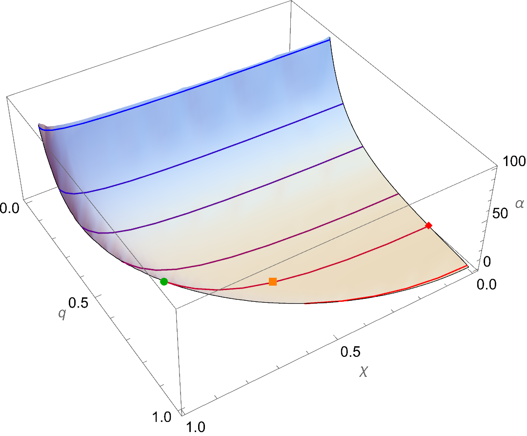
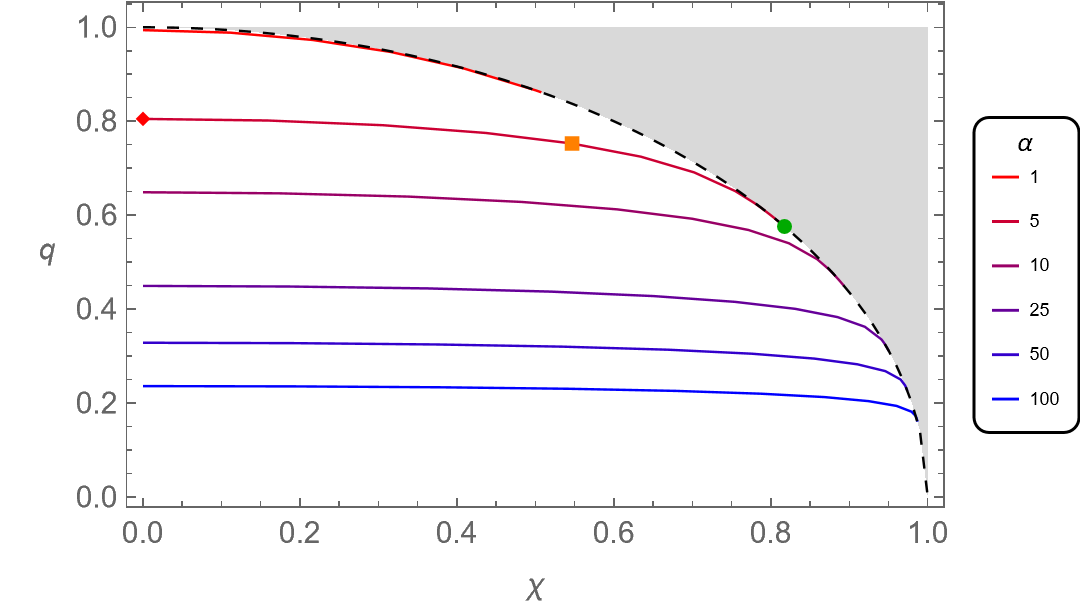
We begin by examining the fundamental mode of scalar clouds with , characterized by nodeless wave functions. Nonlinear realizations of these clouds correspond to scalarized KN black holes in the fundamental state, previously investigated in [64]. The upper-left panel of Fig. 1 depicts the existence domain for the fundamental clouds within the parameter space, where KN black holes supporting such clouds reside on the colored surface. Additionally, existence lines for various fixed values are presented, accompanied by three representative scalar cloud profiles with . The upper-right panel of Fig. 1 illustrates the same existence lines in the plane. The black dashed line represents the extremal limit, corresponding to KN black holes satisfying . The gray region above this extremal line is inaccessible to KN black holes, imposing an upper bound on the black hole charge for a given . As increases, this upper bound decreases from unity to zero. It is noteworthy that the effective mass squared becomes increasingly negative for a given as or grows (cf. Eq. ), signifying an amplification of tachyonic instabilities with larger or values.
Four key characteristics are observed regarding the existence lines:
-
•
Shift Toward Smaller with Increasing : As increases, the existence lines shift towards smaller values. This is attributed to the enhancement of tachyonic instabilities for larger , thereby allowing a lower to induce scalar cloud formation.
-
•
Approach to Extremal Line with Increasing : With increasing , each existence line approaches the extremal line and ultimately terminates at this boundary. Consequently, the charge of the existence lines converges to its upper limit as black hole spin accelerates. This implies that black hole spin suppresses scalar cloud formation, and scalar clouds cease to exist beyond a critical spin, denoted by .
-
•
Threshold Line for Scalarized KN Black Holes: For a given , the corresponding existence line serves as a threshold for scalarized KN black holes. KN black holes below this line exhibit insufficient tachyonic instabilities to support scalar clouds, let alone scalarized black holes, due to their low values. Conversely, KN black holes above the existence line possess excessively strong tachyonic instabilities, necessitating nonlinear effects to suppress these instabilities and give rise to scalarized KN black holes.
-
•
Decrease of Existence Line with Increasing : For a fixed , the existence line exhibits a slight decrease as increases from zero towards the extremal line. At , the value of the existence line, denoted by , corresponds to the bifurcation point of the RN black hole with the given . At the extremal line termination point, the existence line yields a threshold charge, denoted by . Notably, consistently exceeds for fundamental scalar clouds. Tachyonic instabilities of KN black holes with and are too weak and strong, respectively, to allow the existence of scalar clouds.
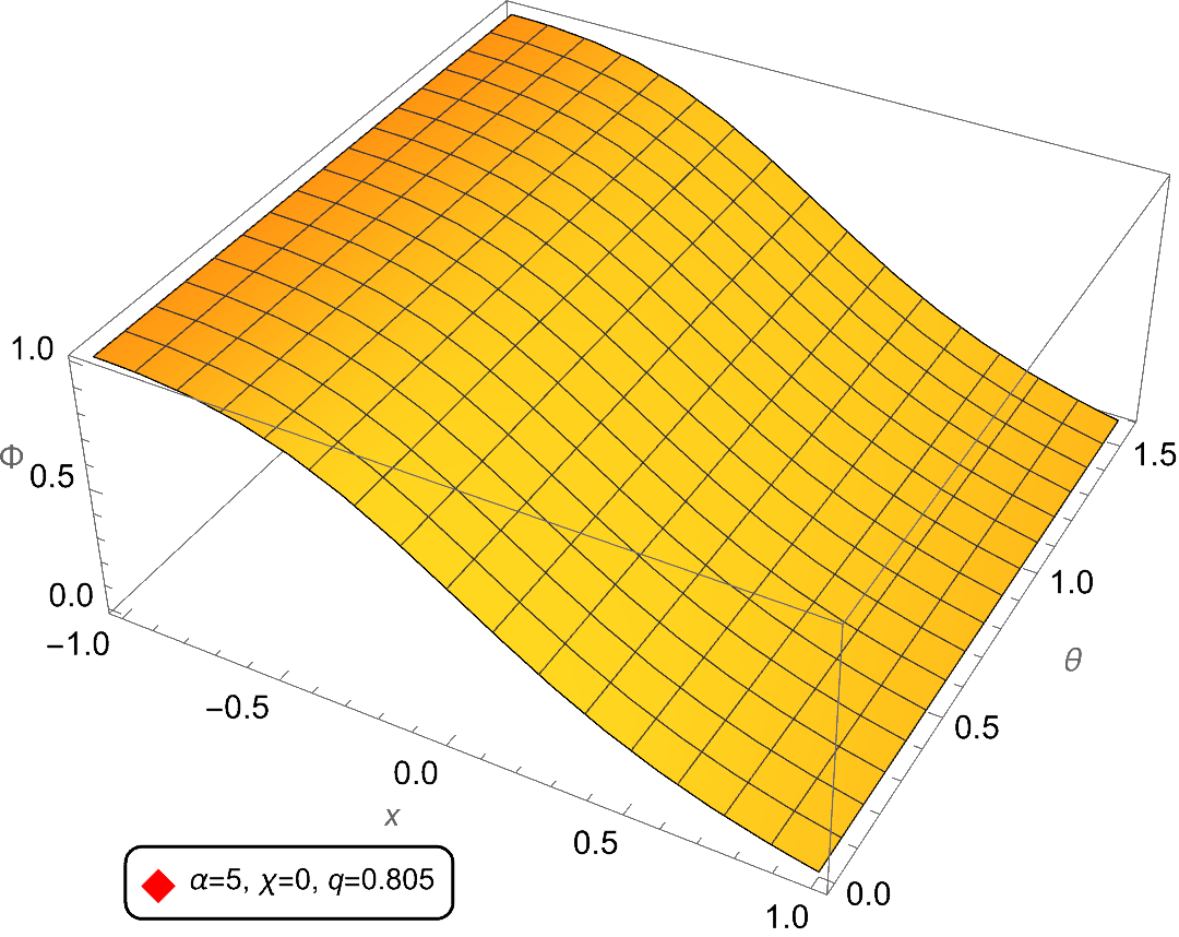
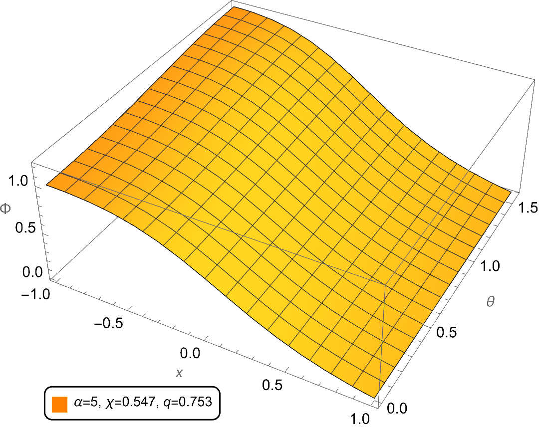
The lower row of Fig. 1 presents the wave function of fundamental scalar clouds for three KN black holes situated on the existence line. The wave function in the lower-left panel corresponds to the RN black hole bifurcation point and exhibits -independence due to the spherical symmetry of RN black holes. The lower-middle and lower-right panels demonstrate a notable elevation of the wave function on the equatorial plane as black hole spin increases. Furthermore, the wave function at the extremal limit displays a sharper peak at the event horizon compared to the cases with zero or moderate spin. These observations collectively indicate that black hole spin induces a concentration of scalar clouds towards both the horizon and the equatorial plane.
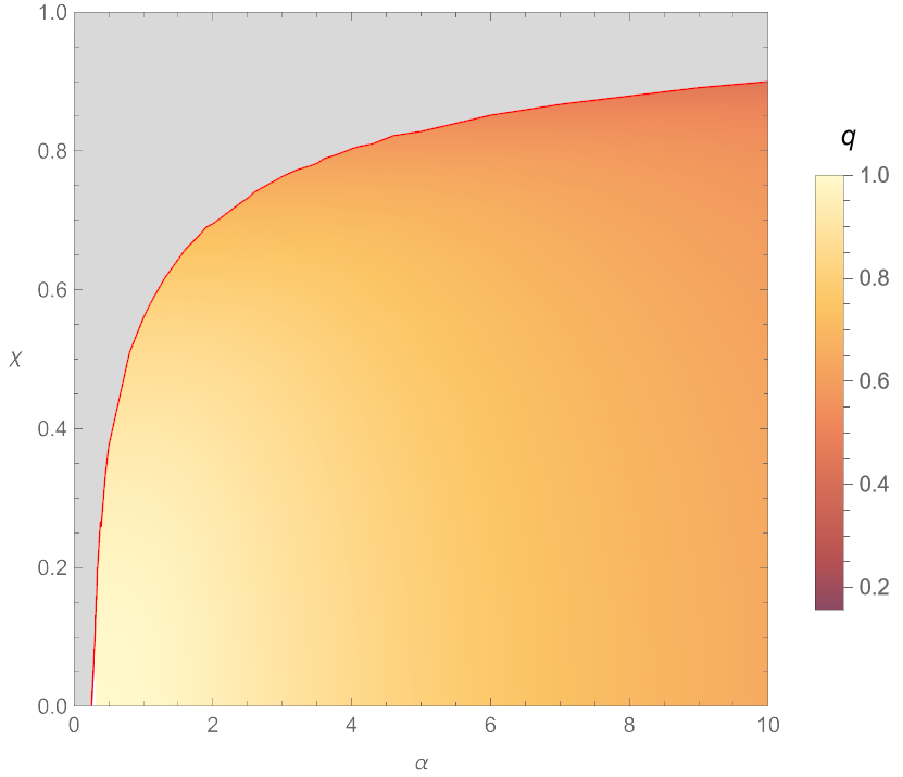
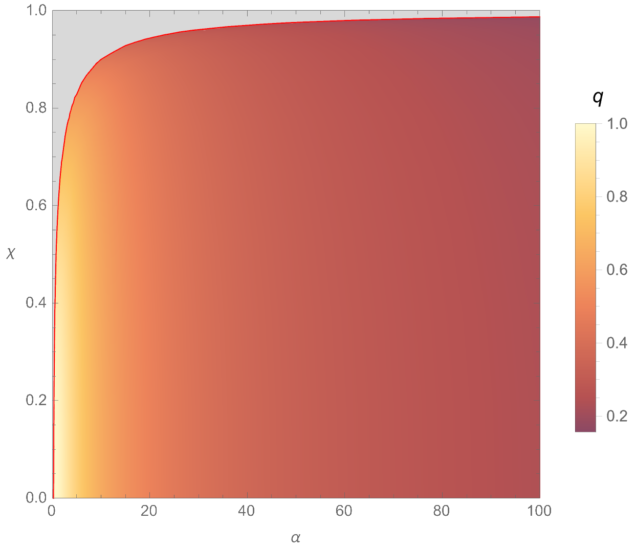
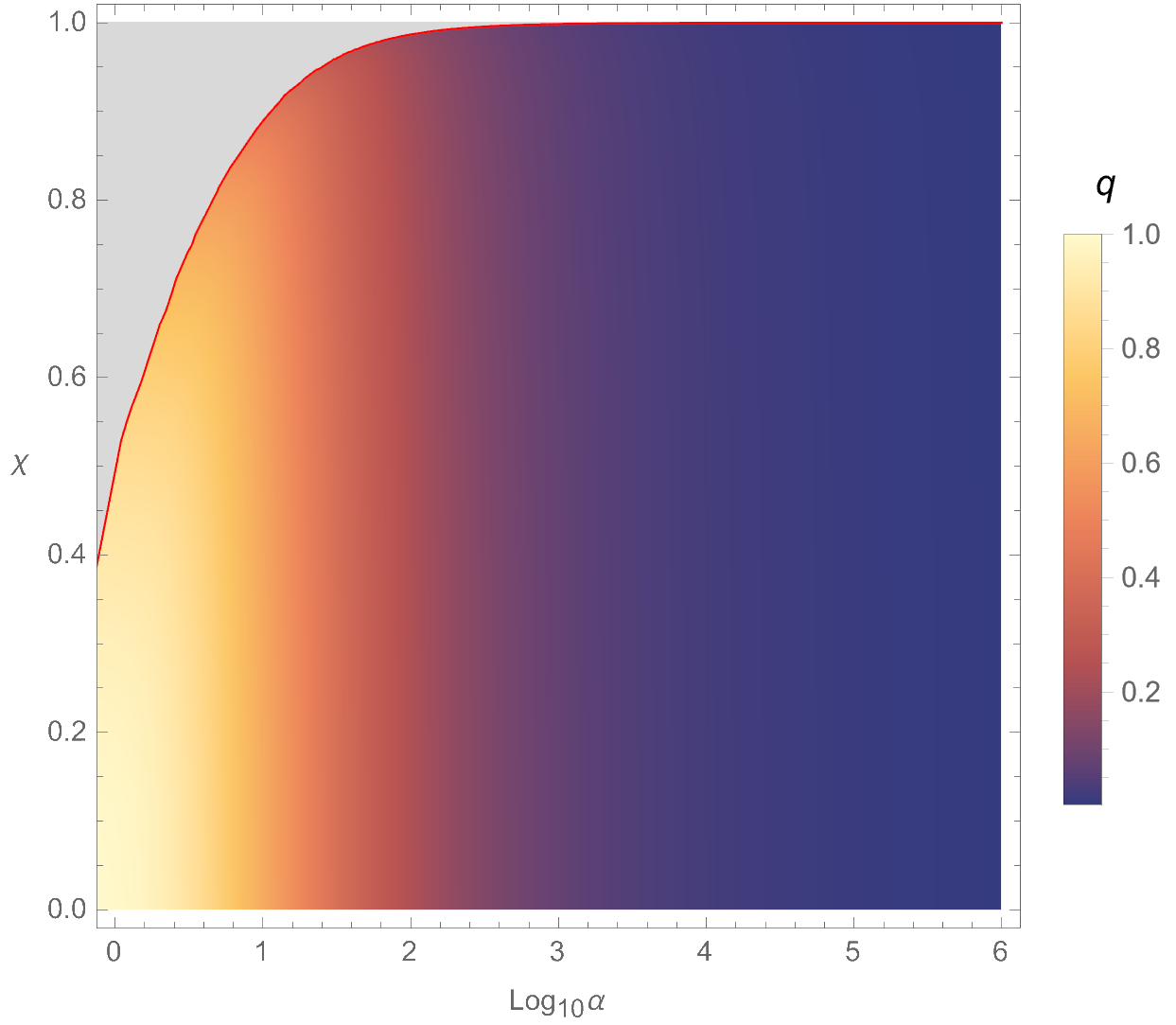
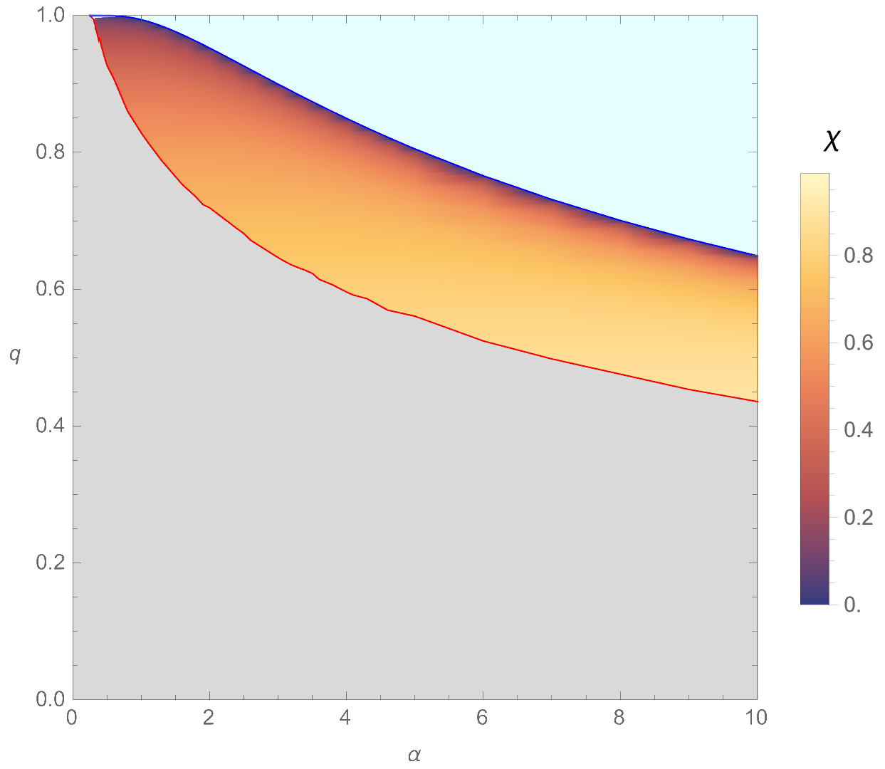
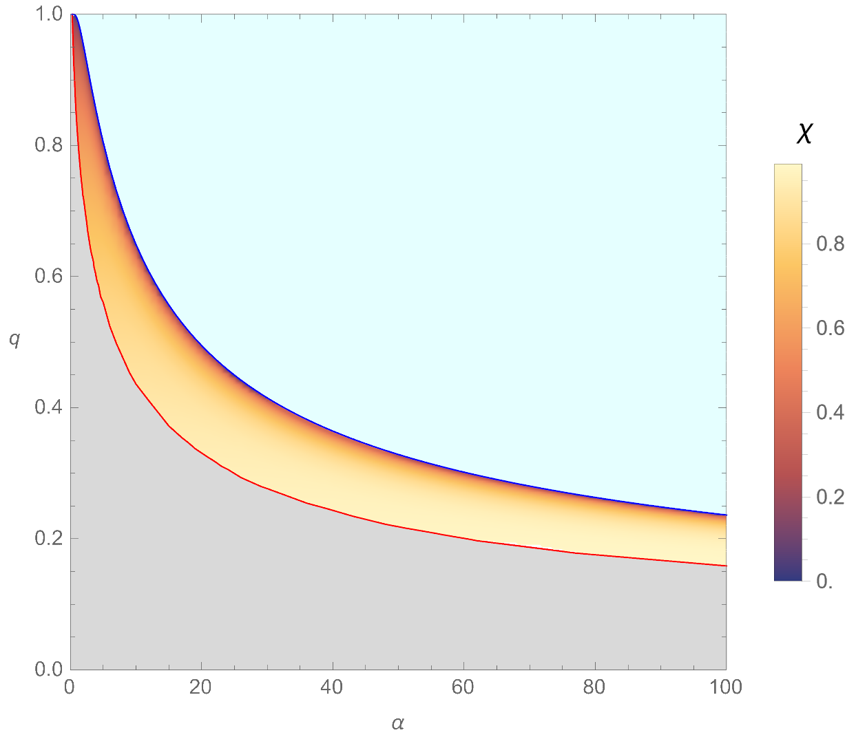
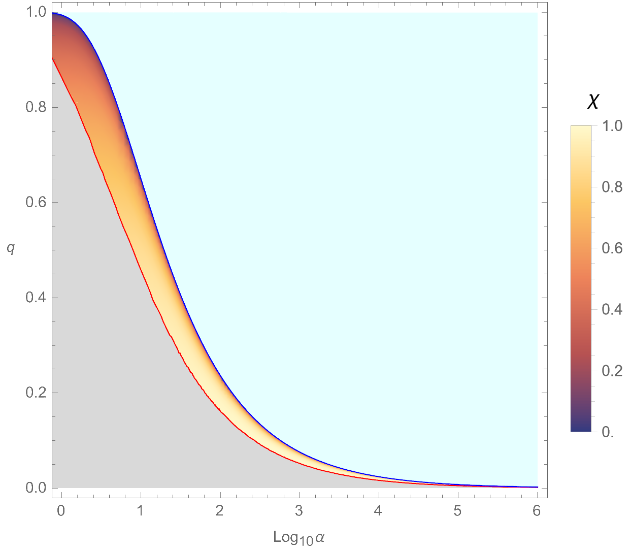
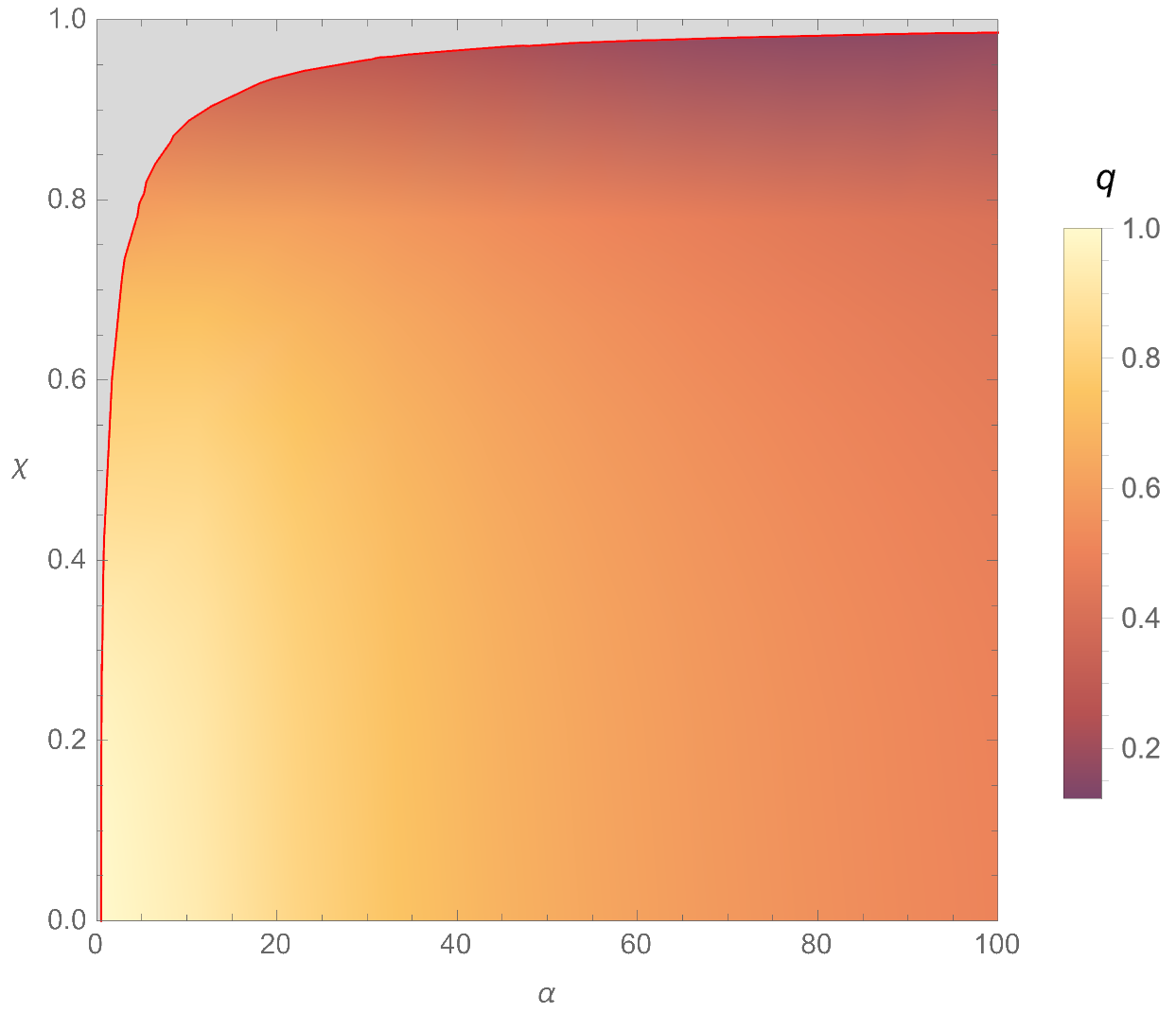
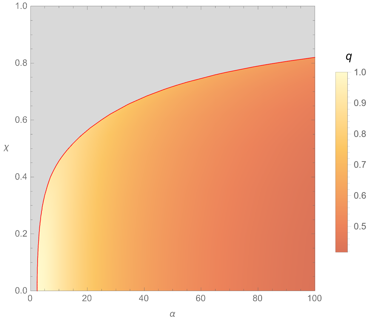
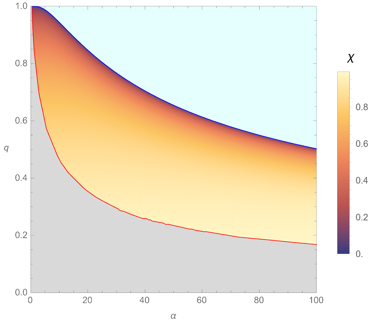
The upper and lower rows of Fig. 2 present density plots of the fundamental cloud existence domain in the and spaces, respectively. Color variations within the density plots indicate corresponding or values. The existence domain in the space is bounded by the upper limit , represented by red lines. Regions above these red lines, denoted as gray, preclude scalar cloud formation as black hole charges must exceed their extremal values to induce sufficient tachyonic instabilities. As anticipated, smaller values are required to sustain scalar clouds for stronger coupling constants . Furthermore, the existence domain in the space is confined by the upper bound , depicted as blue lines, and the lower bound , represented by red lines. Similarly, KN black holes within gray regions below the red lines cannot support scalar clouds due to insufficient tachyonic instabilities. Conversely, cyan regions above the blue line exhibit overly strong tachyonic instabilities to accommodate scalar clouds, leading instead to the emergence of scalarized KN black holes. Moreover, as the coupling constant increases, the fundamental scalar cloud existence region contracts, with both and approaching zero.
IV.2 Excited Modes
The preceding subsection explored the fundamental mode of scalar clouds, whose existence lines mark the onset of fundamental scalarized KN black holes. Analogously, the presence of excited scalar clouds indicates the appearance of scalarized KN black holes in excited states, which remain unexplored. Investigating the existence domain and wave function of excited scalar clouds can illuminate properties of these scalarized black holes. This subsection examines two excited states, specifically those with and .
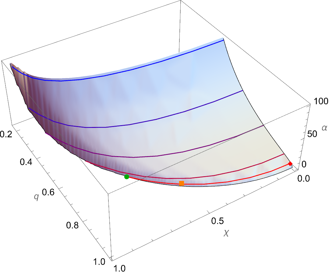
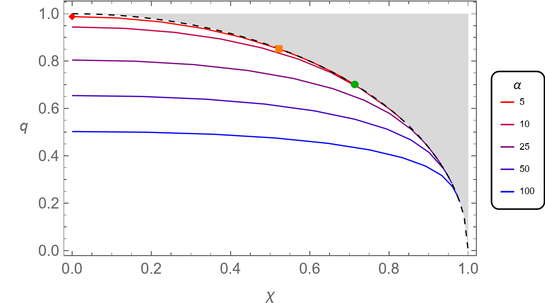
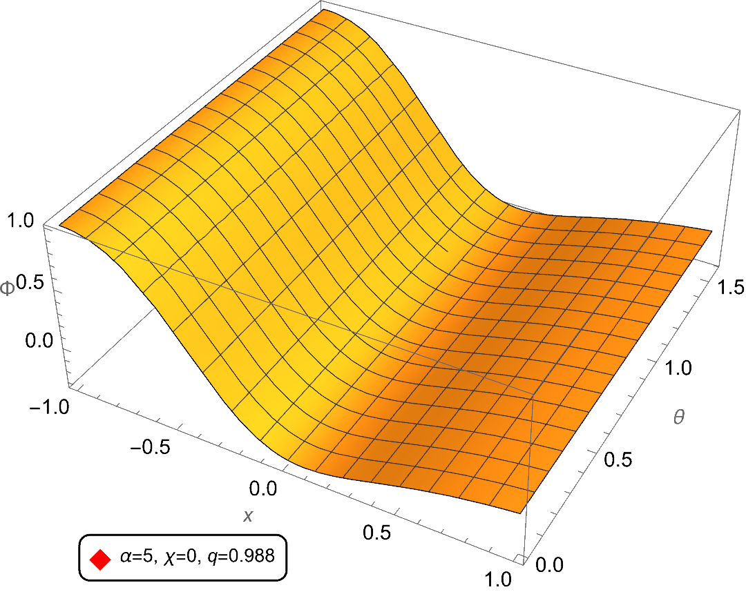
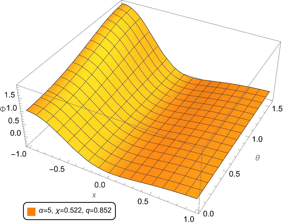
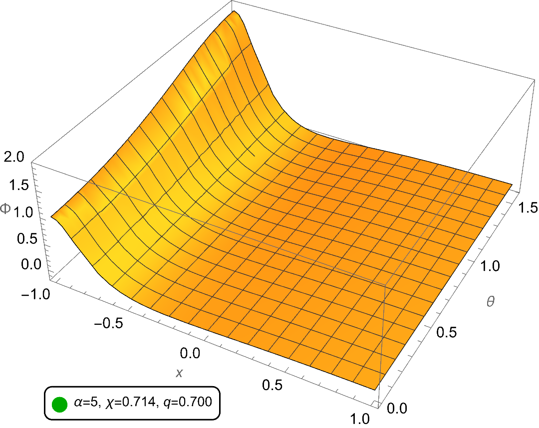
Fig. 3 illustrates the existence domain and wave function of scalar clouds with . The existence surface in the space and existence lines in the space exhibit similarities to the fundamental mode. However, for a given , the excited mode’s existence line lies above that of the fundamental mode, indicating a higher charge requirement (and stronger tachyonic instabilities) for excited scalar cloud formation. The lower row depicts wave functions for three excited clouds with , revealing a valley along the direction due to the presence of a radial node. As black hole spin increases, this valley approaches the event horizon. Similar to fundamental clouds, initially spherically symmetric excited clouds exhibit increased concentration near the equatorial plane with growing spin.
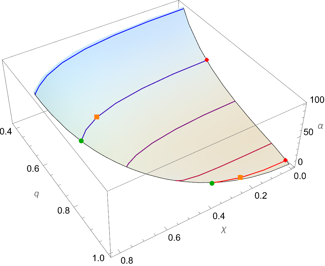
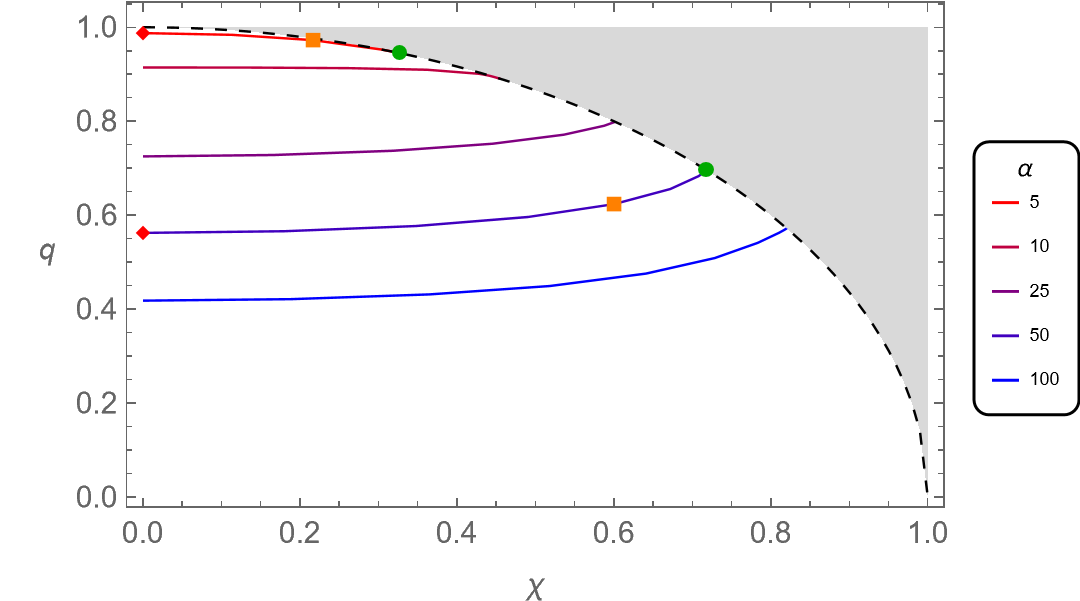
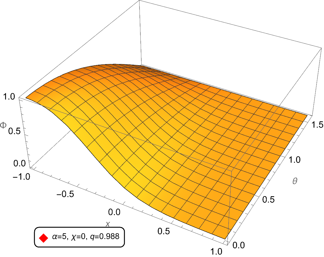
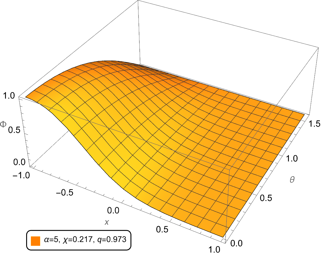
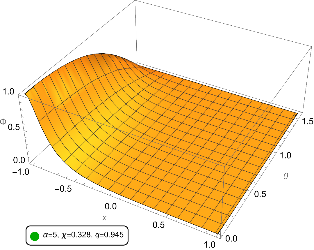
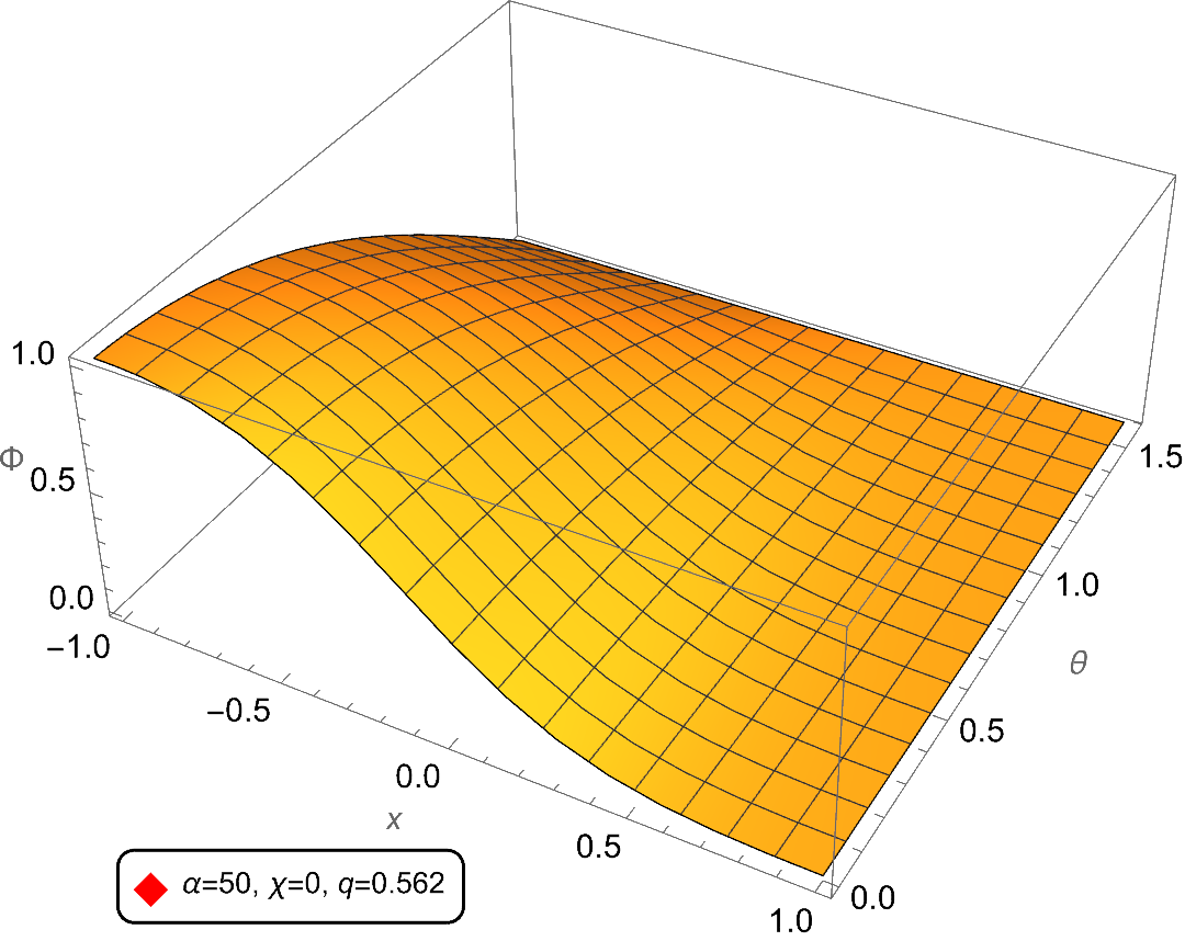
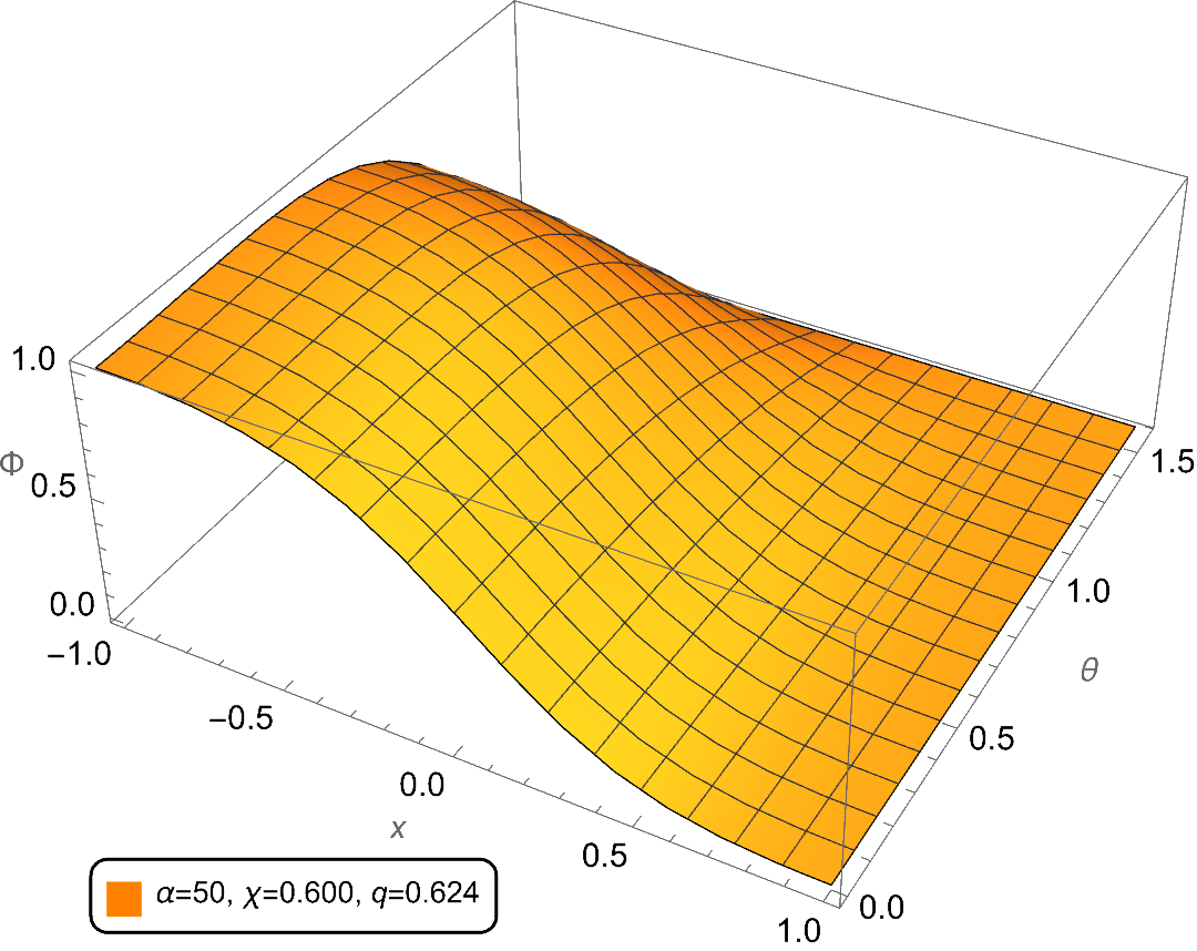
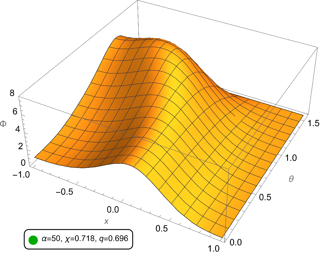
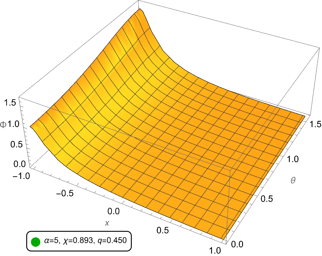
Fig. 4 presents the existence domain and wave function of scalar clouds with . For small (e.g., , ), existence line behavior in the plane resembles that of fundamental and modes. However, for sufficiently large (e.g., , , ), while existence lines still approach and terminate at the extremal line, they exhibit an upward trend with increasing , leading to . The middle row displays wave functions for three representative excited clouds on the existence line, vanishing at due to odd parity. As black hole spin increases, these clouds concentrate towards the event horizon. The lower row presents wave functions for three representative excited clouds with , also vanishing at . Interestingly, a bulge emerges in the scalar clouds with increasing black hole rotation, becoming pronounced near the extremal limit.
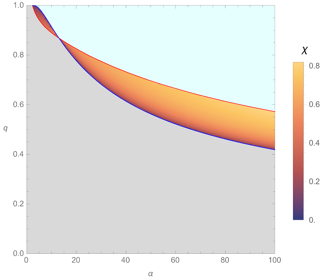
The upper and lower rows of Fig. 5 depict the existence domains of two excited cloud modes in the and spaces, respectively. For comparison, the fundamental cloud’s existence domain is included in the left column. Gray regions indicate insufficient tachyonic instabilities for scalar cloud formation, while cyan regions exhibit excessively strong instabilities preventing stationary scalar clouds. The upper row reveals an upper bound, , on KN black holes supporting scalar clouds. This bound is lower for the mode compared to the modes, implying a requirement for slower black hole spin to accommodate scalar clouds. In the plane, and define the upper and lower limits for clouds. While this holds for small values in the mode, and serve as lower and upper boundaries for large . Notably, gray regions for the excited modes are smaller than those of the fundamental mode, indicating a stronger tachyonic instability threshold for excited scalarized KN black holes.
| N/A | |||||||||
| N/A | |||||||||
| N/A | |||||||||
| N/A | |||||||||
| N/A | N/A | N/A | |||||||
| N/A | N/A | N/A | N/A | N/A | |||||
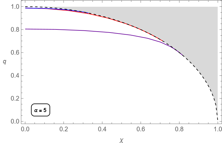
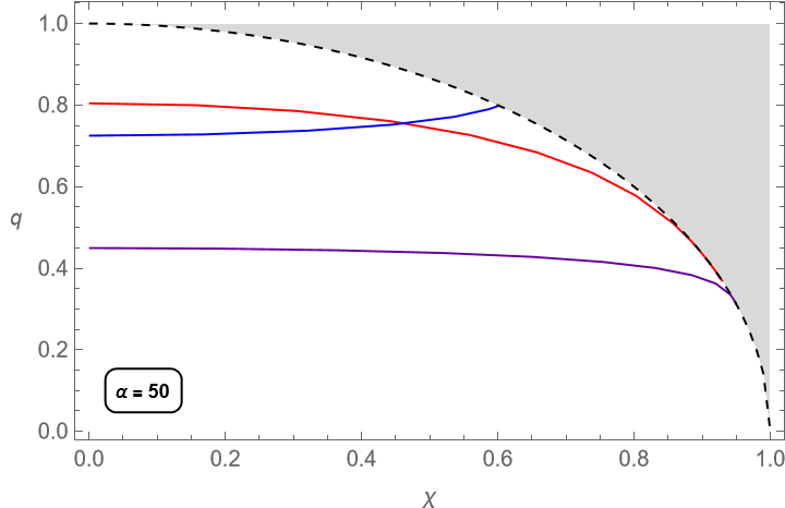
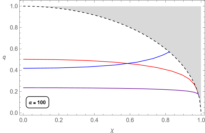
Fig. 6 illustrates the existence lines of fundamental and excited clouds in the plane for , and . Representative and values for each existence line are tabulated in Tab. 1. For all , fundamental cloud existence lines lie below those of excited clouds, indicating a requirement for stronger tachyonic instabilities to form excited clouds. When the coupling constant is weak, excited cloud existence lines primarily reside below those of clouds, suggesting a larger (and stronger tachyonic instabilities) for sustaining clouds. Conversely, for strong , slowly rotating black holes require less charge to support clouds, whereas higher charges are necessary for these clouds when black hole rotation accelerates.
V Conclusions
In this work, we have explored the existence and characteristics of both fundamental and excited scalar clouds in KN black holes. Through a detailed analysis of the parameter space, we identified the regions where these clouds can form and examined how varying the coupling constant , black hole spin and charge influences the formation of these clouds.
For fundamental scalar clouds, our results underscore the influence of the coupling constant and black hole parameters on the cloud’s existence. As expected, larger coupling constants facilitate the formation of these clouds by reducing the required charge. Furthermore, the black hole spin imposes an upper limit on the existence of these clouds, with faster spins leading to a higher charge threshold. Rapidly rotating black holes exhibit a concentration of scalar clouds near the event horizon. In contrast, excited scalar clouds require stronger tachyonic instabilities, as indicated by their existence lines, which consistently lie above those of fundamental clouds. These excited clouds also display unique wave function characteristics, such as valleys that shift toward the event horizon and the emergence of pronounced bulges as the spin increases.
These findings deepen our understanding of scalar cloud dynamics around KN black holes and suggest promising avenues for future research. Excited scalar clouds offer a potential starting point for investigating scalarized KN black holes in excited states. Given the broader applicability of the spectral method, extending our analysis to other rotating black hole solutions is a natural next step. Finally, exploring the astrophysical implications of scalar clouds, particularly within the context of gravitational wave astronomy, presents a compelling research direction.
Acknowledgements.
We are grateful to Yiqian Chen for useful discussions and valuable comments. This work is supported in part by NSFC (Grant No. 12105191, 11947225 and 11875196).References
- [1] Werner Israel. Event horizons in static vacuum space-times. Phys. Rev., 164:1776–1779, 1967. doi:10.1103/PhysRev.164.1776.
- [2] B. Carter. Axisymmetric Black Hole Has Only Two Degrees of Freedom. Phys. Rev. Lett., 26:331–333, 1971. doi:10.1103/PhysRevLett.26.331.
- [3] Remo Ruffini and John A. Wheeler. Introducing the black hole. Phys. Today, 24(1):30, 1971. doi:10.1063/1.3022513.
- [4] Tianshu Wu and Yiqian Chen. Distinguishing the observational signatures of hot spots orbiting Reissner-Nordström spacetime*. Chin. Phys. C, 48(7):075103, 2024. arXiv:2402.06413, doi:10.1088/1674-1137/ad3c2d.
- [5] Deyou Chen, Yiqian Chen, Peng Wang, Tianshu Wu, and Houwen Wu. Gravitational lensing by transparent Janis–Newman–Winicour naked singularities. Eur. Phys. J. C, 84(6):584, 2024. arXiv:2309.00905, doi:10.1140/epjc/s10052-024-12950-z.
- [6] Maximiliano Isi, Matthew Giesler, Will M. Farr, Mark A. Scheel, and Saul A. Teukolsky. Testing the no-hair theorem with GW150914. Phys. Rev. Lett., 123(11):111102, 2019. arXiv:1905.00869, doi:10.1103/PhysRevLett.123.111102.
- [7] Swetha Bhagwat, Xisco Jimenez Forteza, Paolo Pani, and Valeria Ferrari. Ringdown overtones, black hole spectroscopy, and no-hair theorem tests. Phys. Rev. D, 101(4):044033, 2020. arXiv:1910.08708, doi:10.1103/PhysRevD.101.044033.
- [8] Ke Wang. Retesting the no-hair theorem with GW150914. Eur. Phys. J. C, 82(2):125, 2022. arXiv:2111.00953, doi:10.1140/epjc/s10052-022-10049-x.
- [9] M.S. Volkov and D.V. Galtsov. NonAbelian Einstein Yang-Mills black holes. JETP Lett., 50:346–350, 1989.
- [10] P. Bizon. Colored black holes. Phys. Rev. Lett., 64:2844–2847, 1990. doi:10.1103/PhysRevLett.64.2844.
- [11] Brian R. Greene, Samir D. Mathur, and Christopher M. O’Neill. Eluding the no hair conjecture: Black holes in spontaneously broken gauge theories. Phys. Rev. D, 47:2242–2259, 1993. arXiv:hep-th/9211007, doi:10.1103/PhysRevD.47.2242.
- [12] Hugh Luckock and Ian Moss. BLACK HOLES HAVE SKYRMION HAIR. Phys. Lett. B, 176:341–345, 1986. doi:10.1016/0370-2693(86)90175-9.
- [13] Serge Droz, Markus Heusler, and Norbert Straumann. New black hole solutions with hair. Phys. Lett. B, 268:371–376, 1991. doi:10.1016/0370-2693(91)91592-J.
- [14] P. Kanti, N.E. Mavromatos, J. Rizos, K. Tamvakis, and E. Winstanley. Dilatonic black holes in higher curvature string gravity. Phys. Rev. D, 54:5049–5058, 1996. arXiv:hep-th/9511071, doi:10.1103/PhysRevD.54.5049.
- [15] Thomas P. Sotiriou and Shuang-Yong Zhou. Black hole hair in generalized scalar-tensor gravity. Phys. Rev. Lett., 112:251102, 2014. arXiv:1312.3622, doi:10.1103/PhysRevLett.112.251102.
- [16] Adolfo Cisterna and Cristián Erices. Asymptotically locally AdS and flat black holes in the presence of an electric field in the Horndeski scenario. Phys. Rev. D, 89:084038, 2014. arXiv:1401.4479, doi:10.1103/PhysRevD.89.084038.
- [17] G. Antoniou, A. Bakopoulos, and P. Kanti. Evasion of No-Hair Theorems and Novel Black-Hole Solutions in Gauss-Bonnet Theories. Phys. Rev. Lett., 120(13):131102, 2018. arXiv:1711.03390, doi:10.1103/PhysRevLett.120.131102.
- [18] Carlos A.R. Herdeiro and Eugen Radu. Asymptotically flat black holes with scalar hair: a review. Int. J. Mod. Phys. D, 24(09):1542014, 2015. arXiv:1504.08209, doi:10.1142/S0218271815420146.
- [19] Jacob D. Bekenstein. Nonexistence of baryon number for static black holes. Phys. Rev. D, 5:1239–1246, 1972. doi:10.1103/PhysRevD.5.1239.
- [20] J. D. Bekenstein. Transcendence of the law of baryon-number conservation in black hole physics. Phys. Rev. Lett., 28:452–455, 1972. doi:10.1103/PhysRevLett.28.452.
- [21] J. D. Bekenstein. Nonexistence of baryon number for black holes. ii. Phys. Rev. D, 5:2403–2412, 1972. doi:10.1103/PhysRevD.5.2403.
- [22] Carlos A.R. Herdeiro, Eugen Radu, Nicolas Sanchis-Gual, and José A. Font. Spontaneous Scalarization of Charged Black Holes. Phys. Rev. Lett., 121(10):101102, 2018. arXiv:1806.05190, doi:10.1103/PhysRevLett.121.101102.
- [23] Daniela D. Doneva, Stella Kiorpelidi, Petya G. Nedkova, Eleftherios Papantonopoulos, and Stoytcho S. Yazadjiev. Charged Gauss-Bonnet black holes with curvature induced scalarization in the extended scalar-tensor theories. Phys. Rev. D, 98(10):104056, 2018. arXiv:1809.00844, doi:10.1103/PhysRevD.98.104056.
- [24] Pedro V.P. Cunha, Carlos A.R. Herdeiro, and Eugen Radu. Spontaneously Scalarized Kerr Black Holes in Extended Scalar-Tensor–Gauss-Bonnet Gravity. Phys. Rev. Lett., 123(1):011101, 2019. arXiv:1904.09997, doi:10.1103/PhysRevLett.123.011101.
- [25] Carlos A. R. Herdeiro, Eugen Radu, Hector O. Silva, Thomas P. Sotiriou, and Nicolás Yunes. Spin-induced scalarized black holes. Phys. Rev. Lett., 126(1):011103, 2021. arXiv:2009.03904, doi:10.1103/PhysRevLett.126.011103.
- [26] Emanuele Berti, Lucas G. Collodel, Burkhard Kleihaus, and Jutta Kunz. Spin-induced black-hole scalarization in Einstein-scalar-Gauss-Bonnet theory. Phys. Rev. Lett., 126(1):011104, 2021. arXiv:2009.03905, doi:10.1103/PhysRevLett.126.011104.
- [27] Carlos A. R. Herdeiro and Eugen Radu. Kerr black holes with scalar hair. Phys. Rev. Lett., 112:221101, 2014. arXiv:1403.2757, doi:10.1103/PhysRevLett.112.221101.
- [28] Yong-Qiang Wang, Yu-Xiao Liu, and Shao-Wen Wei. Excited Kerr black holes with scalar hair. Phys. Rev. D, 99(6):064036, 2019. arXiv:1811.08795, doi:10.1103/PhysRevD.99.064036.
- [29] Yves Brihaye and Betti Hartmann. Boson stars and black holes with wavy scalar hair. Phys. Rev. D, 105(10):104063, 2022. arXiv:2112.12830, doi:10.1103/PhysRevD.105.104063.
- [30] Ulises Nucamendi and Marcelo Salgado. Scalar hairy black holes and solitons in asymptotically flat space-times. Phys. Rev. D, 68:044026, 2003. arXiv:gr-qc/0301062, doi:10.1103/PhysRevD.68.044026.
- [31] Steven S. Gubser. Phase transitions near black hole horizons. Class. Quant. Grav., 22:5121–5144, 2005. arXiv:hep-th/0505189, doi:10.1088/0264-9381/22/23/013.
- [32] Burkhard Kleihaus, Jutta Kunz, Eugen Radu, and Bintoro Subagyo. Axially symmetric static scalar solitons and black holes with scalar hair. Phys. Lett. B, 725:489–494, 2013. arXiv:1306.4616, doi:10.1016/j.physletb.2013.07.051.
- [33] Asimina Arvanitaki, Savas Dimopoulos, Sergei Dubovsky, Nemanja Kaloper, and John March-Russell. String Axiverse. Phys. Rev. D, 81:123530, 2010. arXiv:0905.4720, doi:10.1103/PhysRevD.81.123530.
- [34] Richard Brito, Shrobana Ghosh, Enrico Barausse, Emanuele Berti, Vitor Cardoso, Irina Dvorkin, Antoine Klein, and Paolo Pani. Stochastic and resolvable gravitational waves from ultralight bosons. Phys. Rev. Lett., 119(13):131101, 2017. arXiv:1706.05097, doi:10.1103/PhysRevLett.119.131101.
- [35] Hooman Davoudiasl and Peter B Denton. Ultralight Boson Dark Matter and Event Horizon Telescope Observations of M87*. Phys. Rev. Lett., 123(2):021102, 2019. arXiv:1904.09242, doi:10.1103/PhysRevLett.123.021102.
- [36] Yifan Chen, Jing Shu, Xiao Xue, Qiang Yuan, and Yue Zhao. Probing Axions with Event Horizon Telescope Polarimetric Measurements. Phys. Rev. Lett., 124(6):061102, 2020. arXiv:1905.02213, doi:10.1103/PhysRevLett.124.061102.
- [37] Yifan Chen, Xiao Xue, Richard Brito, and Vitor Cardoso. Photon Ring Astrometry for Superradiant Clouds. Phys. Rev. Lett., 130(11):111401, 2023. arXiv:2211.03794, doi:10.1103/PhysRevLett.130.111401.
- [38] Yifan Chen, Xiao Xue, and Vitor Cardoso. Black Holes as Neutrino Factories. 8 2023. arXiv:2308.00741.
- [39] Richard Brito, Vitor Cardoso, and Paolo Pani. Superradiance: New Frontiers in Black Hole Physics, volume 906. Springer, 2015. arXiv:1501.06570, doi:10.1007/978-3-319-19000-6.
- [40] Shahar Hod. Kerr-Newman black holes with stationary charged scalar clouds. Phys. Rev. D, 90(2):024051, 2014. arXiv:1406.1179, doi:10.1103/PhysRevD.90.024051.
- [41] Carolina L. Benone, Luís C. B. Crispino, Carlos Herdeiro, and Eugen Radu. Kerr-Newman scalar clouds. Phys. Rev. D, 90(10):104024, 2014. arXiv:1409.1593, doi:10.1103/PhysRevD.90.104024.
- [42] Yang Huang, Dao-Jun Liu, Xiang-Hua Zhai, and Xin-Zhou Li. Scalar clouds around Kerr–Sen black holes. Class. Quant. Grav., 34(15):155002, 2017. arXiv:1706.04441, doi:10.1088/1361-6382/aa7964.
- [43] J. Kunz, I. Perapechka, and Ya. Shnir. Kerr black holes with parity-odd scalar hair. Phys. Rev. D, 100(6):064032, 2019. arXiv:1904.07630, doi:10.1103/PhysRevD.100.064032.
- [44] Nuno M. Santos and Carlos A. R. Herdeiro. Black holes, stationary clouds and magnetic fields. Phys. Lett. B, 815:136142, 2021. arXiv:2102.04989, doi:10.1016/j.physletb.2021.136142.
- [45] Jorge F. M. Delgado, Carlos A. R. Herdeiro, and Eugen Radu. Kerr black holes with synchronized axionic hair. Phys. Rev. D, 103(10):104029, 2021. arXiv:2012.03952, doi:10.1103/PhysRevD.103.104029.
- [46] Vitor Cardoso, Isabella P. Carucci, Paolo Pani, and Thomas P. Sotiriou. Matter around Kerr black holes in scalar-tensor theories: scalarization and superradiant instability. Phys. Rev. D, 88:044056, 2013. arXiv:1305.6936, doi:10.1103/PhysRevD.88.044056.
- [47] Vitor Cardoso, Isabella P. Carucci, Paolo Pani, and Thomas P. Sotiriou. Black holes with surrounding matter in scalar-tensor theories. Phys. Rev. Lett., 111:111101, 2013. arXiv:1308.6587, doi:10.1103/PhysRevLett.111.111101.
- [48] Daniela D. Doneva and Stoytcho S. Yazadjiev. New Gauss-Bonnet Black Holes with Curvature-Induced Scalarization in Extended Scalar-Tensor Theories. Phys. Rev. Lett., 120(13):131103, 2018. arXiv:1711.01187, doi:10.1103/PhysRevLett.120.131103.
- [49] Hector O. Silva, Jeremy Sakstein, Leonardo Gualtieri, Thomas P. Sotiriou, and Emanuele Berti. Spontaneous scalarization of black holes and compact stars from a Gauss-Bonnet coupling. Phys. Rev. Lett., 120(13):131104, 2018. arXiv:1711.02080, doi:10.1103/PhysRevLett.120.131104.
- [50] Guangzhou Guo, Peng Wang, Houwen Wu, and Haitang Yang. Scalarized Einstein–Maxwell-scalar black holes in anti-de Sitter spacetime. Eur. Phys. J. C, 81(10):864, 2021. arXiv:2102.04015, doi:10.1140/epjc/s10052-021-09614-7.
- [51] Hengyu Xu, Yizhi Zhan, and Shao-Jun Zhang. Tachyonic instability and spontaneous scalarization in parameterized Schwarzschild-like black holes. 3 2024. arXiv:2403.19392.
- [52] Thibault Damour and Gilles Esposito-Farese. Nonperturbative strong field effects in tensor - scalar theories of gravitation. Phys. Rev. Lett., 70:2220–2223, 1993. doi:10.1103/PhysRevLett.70.2220.
- [53] Qingyu Gan, Peng Wang, Houwen Wu, and Haitang Yang. Photon spheres and spherical accretion image of a hairy black hole. Phys. Rev. D, 104(2):024003, 2021. arXiv:2104.08703, doi:10.1103/PhysRevD.104.024003.
- [54] Qingyu Gan, Peng Wang, Houwen Wu, and Haitang Yang. Photon ring and observational appearance of a hairy black hole. Phys. Rev. D, 104(4):044049, 2021. arXiv:2105.11770, doi:10.1103/PhysRevD.104.044049.
- [55] Guangzhou Guo, Xin Jiang, Peng Wang, and Houwen Wu. Gravitational lensing by black holes with multiple photon spheres. Phys. Rev. D, 105(12):124064, 2022. arXiv:2204.13948, doi:10.1103/PhysRevD.105.124064.
- [56] Yiqian Chen, Guangzhou Guo, Peng Wang, Houwen Wu, and Haitang Yang. Appearance of an infalling star in black holes with multiple photon spheres. Sci. China Phys. Mech. Astron., 65(12):120412, 2022. arXiv:2206.13705, doi:10.1007/s11433-022-1986-x.
- [57] Yiqian Chen, Peng Wang, and Haitang Yang. Interferometric Signatures of Black Holes with Multiple Photon Spheres. 12 2023. arXiv:2312.10304.
- [58] Yiqian Chen, Peng Wang, and Haitang Yang. Observations of orbiting hot spots around scalarized Reissner–Nordström black holes. Eur. Phys. J. C, 84(3):270, 2024. arXiv:2401.10905, doi:10.1140/epjc/s10052-024-12635-7.
- [59] Guangzhou Guo, Peng Wang, Houwen Wu, and Haitang Yang. Quasinormal modes of black holes with multiple photon spheres. JHEP, 06:060, 2022. arXiv:2112.14133, doi:10.1007/JHEP06(2022)060.
- [60] Guangzhou Guo, Peng Wang, Houwen Wu, and Haitang Yang. Echoes from hairy black holes. JHEP, 06:073, 2022. arXiv:2204.00982, doi:10.1007/JHEP06(2022)073.
- [61] Guangzhou Guo, Peng Wang, Houwen Wu, and Haitang Yang. Superradiance instabilities of charged black holes in Einstein-Maxwell-scalar theory. JHEP, 07:070, 2023. arXiv:2301.06483, doi:10.1007/JHEP07(2023)070.
- [62] Guangzhou Guo, Peng Wang, and Yupeng Zhang. Nonlinear Stability of Black Holes with a Stable Light Ring. 3 2024. arXiv:2403.02089.
- [63] Guangzhou Guo, Yuhang Lu, Peng Wang, Houwen Wu, and Haitang Yang. Black holes with multiple photon spheres. Phys. Rev. D, 107(12):124037, 2023. arXiv:2212.12901, doi:10.1103/PhysRevD.107.124037.
- [64] Guangzhou Guo, Peng Wang, Houwen Wu, and Haitang Yang. Scalarized Kerr-Newman black holes. JHEP, 10:076, 2023. arXiv:2307.12210, doi:10.1007/JHEP10(2023)076.
- [65] Pedro G. S. Fernandes, Carlos A. R. Herdeiro, Alexandre M. Pombo, Eugen Radu, and Nicolas Sanchis-Gual. Spontaneous Scalarisation of Charged Black Holes: Coupling Dependence and Dynamical Features. Class. Quant. Grav., 36(13):134002, 2019. [Erratum: Class.Quant.Grav. 37, 049501 (2020)]. arXiv:1902.05079, doi:10.1088/1361-6382/ab23a1.
- [66] Shahar Hod. Spontaneous scalarization of charged Reissner-Nordstr\”om black holes: Analytic treatment along the existence line. Phys. Lett. B, 798:135025, 2019. arXiv:2002.01948.
- [67] S. A. Teukolsky. Rotating black holes - separable wave equations for gravitational and electromagnetic perturbations. Phys. Rev. Lett., 29:1114–1118, 1972. doi:10.1103/PhysRevLett.29.1114.
- [68] Saul A. Teukolsky. Perturbations of a rotating black hole. 1. Fundamental equations for gravitational electromagnetic and neutrino field perturbations. Astrophys. J., 185:635–647, 1973. doi:10.1086/152444.
- [69] S. A. Teukolsky and W. H. Press. Perturbations of a rotating black hole. III - Interaction of the hole with gravitational and electromagnet ic radiation. Astrophys. J., 193:443–461, 1974. doi:10.1086/153180.
- [70] John P Boyd. Chebyshev and Fourier spectral methods. Courier Corporation, 2001.
- [71] Pedro G. S. Fernandes and David J. Mulryne. A new approach and code for spinning black holes in modified gravity. Class. Quant. Grav., 40(16):165001, 2023. arXiv:2212.07293, doi:10.1088/1361-6382/ace232.
- [72] Meng-Yun Lai, De-Cheng Zou, Rui-Hong Yue, and Yun Soo Myung. Nonlinearly scalarized rotating black holes in Einstein-scalar-Gauss-Bonnet theory. 4 2023. arXiv:2304.08012.
- [73] Clare Burrage, Pedro G. S. Fernandes, Richard Brito, and Vitor Cardoso. Spinning Black Holes with Axion Hair. 6 2023. arXiv:2306.03662.
- [74] Aron Jansen. Overdamped modes in Schwarzschild-de Sitter and a Mathematica package for the numerical computation of quasinormal modes. Eur. Phys. J. Plus, 132(12):546, 2017. arXiv:1709.09178, doi:10.1140/epjp/i2017-11825-9.
- [75] Qingyu Gan, Guangzhou Guo, Peng Wang, and Houwen Wu. Strong cosmic censorship for a scalar field in a Born-Infeld–de Sitter black hole. Phys. Rev. D, 100(12):124009, 2019. arXiv:1907.04466, doi:10.1103/PhysRevD.100.124009.
- [76] Adrian Ka-Wai Chung, Pratik Wagle, and Nicolas Yunes. Spectral method for the gravitational perturbations of black holes: Schwarzschild background case. Phys. Rev. D, 107(12):124032, 2023. arXiv:2302.11624, doi:10.1103/PhysRevD.107.124032.
- [77] Adrian Ka-Wai Chung, Pratik Wagle, and Nicolas Yunes. Spectral method for metric perturbations of black holes: Kerr background case in general relativity. Phys. Rev. D, 109(4):044072, 2024. arXiv:2312.08435, doi:10.1103/PhysRevD.109.044072.
- [78] Adrian Ka-Wai Chung and Nicolas Yunes. Ringing out General Relativity: Quasi-normal mode frequencies for black holes of any spin in modified gravity. 5 2024. arXiv:2405.12280.