Learning to Optimally Stop a Diffusion Process

Abstract

We study optimal stopping for a diffusion process with unknown model primitives within the continuous-time reinforcement learning (RL) framework developed by Wang et al., (2020). By penalizing its variational inequality, we transform the stopping problem into a stochastic optimal control problem with two actions. We then randomize control into Bernoulli distributions and add an entropy regularizer to encourage exploration. We derive a semi-analytical optimal Bernoulli distribution, based on which we devise RL algorithms using the martingale approach established in Jia and Zhou, 2022a and prove a policy improvement theorem. Finally, we demonstrate the effectiveness of the algorithms in examples of pricing finite-horizon American put options and solving Merton’s problem with transaction costs, and show that both the offline and online algorithms achieve high accuracy in learning the value functions and characterizing the associated free boundaries.

Keywords: Optimal stopping, reinforcement learning, HJB equation, penalty method, martingale, free boundary, policy improvement.

1 Introduction

Optimal stopping involves making decisions on the best timing to exit (or enter) an endeavor with an immediate payoff when waiting for a higher payoff in the future is no longer beneficial. Such problems abound in many applications, including finance, physics, and engineering. A prominent example is the pricing of an American-type option where one needs to decide when to exercise the right to buy or sell an underlying stock.

Optimal stopping can be regarded as a control problem in which there are only two control actions: stop (exit) or wait (continue). Yet historically, the optimal stopping theory has been developed fairly separately from that of the general optimal control, owing to the very specific nature of the former, even though both are based on the fundamentally same approaches, namely martingale theory and dynamic programming (DP). For optimal stopping with a continuous-time diffusion process, DP leads to a free-boundary PDE (also known as variational inequality) that, if solved, can be used to characterize the stopping/continuation regions in the time–state space and to obtain the optimal value of the problem.

However, there are two issues with the classical approach to optimal stopping, one conceptual and one technical. The first one is that the free-boundary PDE is available only when the model primitives are known and given, while in many applications model primitives are often hard to estimate to the desired accuracy or are simply unavailable. The second issue is that even if the model is completely known and the PDE is available, solving it by traditional numerical PDE methods (e.g., the finite difference method) in high dimensions is notoriously difficult due to the curse of dimensionality.

This is where continuous-time reinforcement learning (RL) comes to the rescue. RL has been developed to solve dynamic optimization in partially or completely unknown environments. This is achieved through interacting with and exploring the environment: the RL agent tries different actions strategically and observes responses from the environment, based on which she learns to improve her action plans. A key to the success of this process is to carefully balance exploration (learning) and exploitation (optimization). RL is also a powerful way to deal with the curse of dimensionality, because it no longer attempts to solve dynamic programming equations; rather it employs Monte Carlo and stochastic gradient descent to compute policies and values, which is less prone to the dimensionality complexity (e.g., Han et al., (2018)).

While RL for discrete-time Markov decision processes (MDPs) has been developed for a long time (Sutton and Barto,, 1999), recently the study of RL for controlled continuous-time diffusion processes has drawn increasing attention, starting from Wang et al., (2020). Continuous RL problems are important because many practical problems are naturally continuous in time (and in space). While one can discretize time upfront and turn a continuous-time problem into a discrete-time MDP, it has been experimentally shown (e.g., Munos,, 2006; Tallec et al.,, 2019) that this approach is very sensitive to time discretization and performs poorly with small time steps. Equally important, there are more mathematical tools available for the continuous setting that make it possible to establish an overarching and rigorous theoretical foundation for RL algorithms, as demonstrated in a series of papers Jia and Zhou, 2022a ; Jia and Zhou, 2022b ; Jia and Zhou, (2023). Indeed, the study on continuous RL may provide new perspectives even for discrete-time MDPs. The general theory has already found applications in finance, including dynamic mean–variance analysis (Wang and Zhou,, 2020; Dai et al.,, 2023; Wu and Li,, 2024) and Merton’s problem (Jiang et al.,, 2022; Dai et al.,, 2023; Dai and Dong,, 2024).

This paper studies optimal stopping in a finite time horizon for a (potentially high-dimensional) diffusion process with unknown model parameters. Instead of developing an RL theory for optimal stopping from the ground up parallel to the control counterpart (Wang et al.,, 2020; Jia and Zhou, 2022a, ; Jia and Zhou, 2022b, ; Jia and Zhou,, 2023), we first transform the stopping problem into a stochastic control problem, inspired by Dai et al., (2007). Indeed this transformation is motivated by the fact that the free-boundary PDE can be approximated by a “penalized” PDE, whose solution converges to that of the original PDE as the penalty parameter approaches infinity (Friedman,, 1982; Forsyth and Vetzal,, 2002; Liang et al.,, 2007; Peng et al.,, 2024). Moreover, the penalized PDE is actually the Hamilton-Jacobi-Bellman (HJB) equation of a stochastic bang-bang control problem.

Once we have turned the problem into an RL problem for stochastic control, we can apply/adapt all the available results, methods and algorithms developed for the latter right away. In particular, we take the exploratory formulation of Wang et al., (2020) involving control randomization and entropy regularization. Because the control set now contains only two actions (corresponding to stop and continuation), the randomized control is a Bernoulli distribution. In other words, for exploring the environment there is no longer a clear-cut stop or continuation decision. Rather, the agent designs a (biased) coin for each time–state pair and makes the stopping decision based on the outcome of a coin toss. Moreover, we derive a semi-analytical formula for the optimal Bernoulli distribution, which is crucial for policy parameterization and policy improvement in designing our RL algorithms. Built upon the martingale approach established by Jia and Zhou, 2022a , we design two RL algorithms: an offline martingale loss (ML) algorithm and an online TD(0) algorithm. We then present simulations of applying these algorithms to the problems of pricing a finite-horizon American put option and of solving Merton’s portfolio choice with transaction costs.

This work is closely related to Dong, (2024), the first paper in the literature to study optimal stopping within the continuous-time exploratory framework of Wang et al., (2020). However, there are stark differences. First, we turn the stopping problem into a stochastic control problem using the penalty method, while Dong, (2024) treats the stopping problem directly by randomizing stopping times with a Cox process. The advantage of our approach, as already noted earlier, is that once in the control formulation, we can immediately apply all the available RL theories for controlled diffusions developed so far, instead of having to develop the corresponding theories for stopping from the get-go. Second, the entropy regularizers are chosen differently. We adopt the usual Shannon differential entropy, also used by Wang et al., (2020) and its sequel, while Dong, (2024) employs the so-called unnormalized negentropy. See Section 4.6 for a more detailed discussion on this point. Finally, in our experiments, we examine the performance of our methods with both online and offline algorithms, while Dong, (2024) only shows his offline results.

This work is also related to a strand of papers on machine learning for optimal stopping (e.g., Becker et al.,, 2019, 2020, 2021; Reppen et al.,, 2022; Herrera et al.,, 2024; Peng et al.,, 2024). These papers focus on using deep neural nets to approximate the free boundaries and/or optimal stopping, significantly outside the entropy-regularized, exploratory framework of Wang et al., (2020) to which the present paper belongs.

The remainder of the paper is organized as follows. Section 2 transforms the optimal stopping problem with a finite horizon into a bang-bang stochastic control problem and then presents its exploratory formulation. In Section 3, we propose both the online and offline RL algorithms and provide a policy improvement theorem. Section 4 is devoted to simulation studies on pricing an American put option and on an investment problem with transaction costs. Finally, Section 5 concludes. All the proofs and additional materials are presented in the appendices.

2 Optimal stopping in finite time horizon

We fix a filtered probability space $(\Omega,\mathcal{F},\mathbb{P};\left\{\mathcal{F}_{t}\right\}_{t\geqslant 0})$ in which a standard $d$-dimensional Brownian motion $W=(W^{(1)},W^{(2)},\cdots,W^{(d)})$ is defined, along with a time horizon $T>0$. Consider the following optimal stopping problem with a finite horizon

$$\max_{\tau\in[0,T]}\operatorname{\mathbb{E}}\!\left[g(\tau,X_{\tau})\right]$$ (2.1)

for an $n$-dimensional diffusion process $X=(X^{(1)},X^{(2)},\cdots,X^{(n)})$ driven by

$$\operatorname{d}\!X^{(i)}_{t}=b_{i}(t,X_{t})\operatorname{d}\!t+\sum_{j}\sigma_{i,j}(t,X_{t})\operatorname{d}\!W^{(j)}_{t}.$$ (2.2)

It is well-known that the HJB equation of problem (2.1) is given by

$$\begin{cases}\max\{v_{t}+\mathscr{L}v,g-v\}=0,\ (t,x)\in[0,T)\times\operatorname{\mathbb{R}}^{n},\\ v(T,x)=g(T,x),\end{cases}$$ (2.3)

where

$$\mathscr{L}v(t,x)=\frac{1}{2}\sum_{i,j,k}\sigma_{i,k}(t,x)\sigma_{j,k}(t,x)\frac{\partial^{2}v}{\partial x_{i}\partial x_{j}}+\sum_{i}b_{i}(t,x)\frac{\partial v}{\partial x_{i}}.$$ (2.4)

Throughout this paper, we assume all the coefficients are continuous in $t$ and Lipschitz continuous in $x$. Moreover, $\sigma\sigma^{\prime}$ is uniformly bounded and positive definite, where $\sigma=(\sigma_{i,j})_{i,j}$.

2.1 Penalty approximation

Consider the following penalty approximation problem for (2.3):

$$\begin{cases}v_{t}+\mathscr{L}v+K(g-v)^{+}=0,\ (t,x)\in[0,T)\times\operatorname{\mathbb{R}}^{n},\\ v(T,x)=g(T,x),\end{cases}$$ (2.5)

where $K$ is a positive scalar, called the penalty factor. The following result states the relationship between (2.5) and (2.3).

Lemma 2.1.

The solution of (2.5) converges to that of (2.3) as $K\to+\infty$.

A proof of this lemma can be found in the literature such as Friedman, (1982), Liang et al., (2007), and Peng et al., (2024). Indeed, one can obtain the following estimate:

$$0\leqslant v(t,x)-v^{K}(t,x)\leqslant\frac{C}{K},~{}~{}\forall\;(t,x,K)\in[0,T]\times\operatorname{\mathbb{R}}^{n}\times(0,\infty)$$

under some technical conditions, where $v$ and $v^{K}$ are respectively the solutions to (2.3) and (2.5), and $C$ is a positive constant. For reader’s convenience we will provide a proof of Lemma 2.1 in Appendix A.1.

Lemma 2.1 suggests that solving (2.3) reduces to solving (2.5) with a sufficiently large $K$. In particular, numerically one can simply solve the latter to get an approximated solution to the former. We can rewrite (2.5) as the following PDE involving a binary optimization term

$$0 =v_{t}+\mathscr{L}v+K(g-v)^{+}=v_{t}+\max_{u\in\{0,1\}}\{\mathscr{L}v-Kuv+Kg(t,x)u\}.$$ (2.6)

We are now going to show in the next subsection that this PDE corresponds to some (unconventional) stochastic control problem.

2.2 Transformation to optimal control

Before we further analyze (2.6), let us first consider the following general stochastic control problem

$$v(s,x)=\max_{u\in\mathscr{U}}J(s,x;u),$$ (2.7)

where the controlled $n$-dimensional process $X_{t}$ follows

$$\operatorname{d}\!X_{t}=\tilde{b}(t,X_{t},u_{t})\operatorname{d}\!t+\tilde{\sigma}(t,X_{t},u_{t})\operatorname{d}\!W_{t},$$ (2.8)

and the objective functional (also called the reward function in the RL literature) is defined as

$$J(s,x;u)=\operatorname{\mathbb{E}}\!\left[\int_{s}^{T}e^{-\int_{s}^{t}f(r,X_{r},u_{r})\operatorname{d}\!r}G(t,X_{t},u_{t})\operatorname{d}\!t+e^{-\int_{s}^{T}f(r,X_{r},u_{r})\operatorname{d}\!r}H(X_{T})\;\bigg{|}\;X_{s}=x\right].$$

Here $\mathscr{U}$ denotes the set of admissible controls $u:[0,T]\times\Omega\to U$ which are progressively measurable such that (2.8) admits a unique strong solution and $J(s,x;u)$ is finite, while $U\subseteq\operatorname{\mathbb{R}}^{m}$ is the closed control constraint set.

Note that this is not a conventional stochastic control problem (e.g., Yong and Zhou, (1999)) as it involves control-dependent discount factors. However, we still have the following HJB equation and verification theorem.

Theorem 2.2 (Verification theorem).

Suppose $v$ is a classical solution of

$$\begin{cases}v_{t}+\max_{u\in U}\left\{\mathscr{L}_{u}v-vf+G\right\}=0,~{}~{}(t,x)\in[0,T)\times\operatorname{\mathbb{R}}^{n},\\ v(T,x)=H(x),\end{cases}$$ (2.9)

where

$$\mathscr{L}_{u}v=\frac{1}{2}\sum_{i,j,k}\tilde{\sigma}_{i,k}(t,x,u)\tilde{\sigma}_{j,k}(t,x,u)\frac{\partial^{2}v}{\partial x_{i}\partial x_{j}}+\sum_{i}\tilde{b}_{i}(t,x,u)\frac{\partial v}{\partial x_{i}}.$$

Then it is the value function of problem (2.7).

Remark 2.1.

If $f$ is a constant, then the above result reduces to the classical verification theorem. One can indeed establish a similar result when a term like $e^{-\int_{s}^{t}f(r,X_{r},u_{r})\operatorname{d}\!r-\int_{s}^{t}g(r,X_{r},u_{r})\operatorname{d}\!W_{r}}$ is in place of $e^{-\int_{s}^{t}f(r,X_{r},u_{r})\operatorname{d}\!r}$ in the reward functional $J$.

By Theorem 2.2, the PDE (2.6) is indeed the HJB equation for the following stochastic control problem:

$$v(s,x)=\max_{u_{t}\in\{0,1\}}J(s,x;u),$$ (2.10)

where the (uncontrolled) process $X_{t}$ is driven by (2.2) and

$$J(s,x;u)=\operatorname{\mathbb{E}}\!\left[\int_{s}^{T}Ke^{-K\int_{s}^{t}u_{r}\operatorname{d}\!r}g(t,X_{t})u_{t}\operatorname{d}\!t+e^{-K\int_{s}^{T}u_{r}\operatorname{d}\!r}g(T,X_{T})\;\bigg{|}\;X_{s}=x\right].$$ (2.11)

Applying Theorem 2.2 yields

Lemma 2.3.

Suppose $v$ is a classical solution of (2.6) with terminal condition $v(T,x)=g(T,x)$. Then it is the value function of problem (2.10).

Even though we have established the theoretical dynamic programming result for the non-conventional control problem (2.10), we hope to turn the problem into a conventional one so that we can treat it with the widely and immediately available methods for classical controls. This can be achieved by introducing an additional state.

Recall that $X_{t}$ is driven by (2.2); introduce a new controlled state equation $\operatorname{d}\!R_{t}=-KR_{t}u_{t}\operatorname{d}\!t$ or $R_{t}=R_{s}e^{-K\int_{s}^{t}u_{r}\operatorname{d}\!r}$ for $t\geqslant s$. Let

$$\bar{v}(s,x,r)=\max_{u_{t}\in\{0,1\}}\bar{J}(s,x,r;u),$$ (2.12)

where

$$\bar{J}(s,x,r;u)=\operatorname{\mathbb{E}}\!\left[\int_{s}^{T}KR_{t}g(t,X_{t})u_{t}\operatorname{d}\!t+R_{T}g(T,X_{T})\;\bigg{|}\;X_{s}=x,R_{s}=r\right].$$

Then clearly problem (2.10) has the optimal value $v(s,x)=\bar{v}(s,x,1).$

As is well known, the HJB equation for the classical control problem (2.12) is given by

$$\begin{cases}\displaystyle{\bar{v}_{t}+\max_{u\in\{0,1\}}\Big{[}\mathscr{L}\bar{v}-Kru\frac{\partial\bar{v}}{\partial r}+Krg(t,x)u\Big{]}=0,\ (t,x,r)\in[0,T)\times\operatorname{\mathbb{R}}^{n}\times(0,\infty),}\\ \bar{v}(T,x,r)=rg(T,x),~{}~{}\bar{v}(t,x,0)=0.\end{cases}$$ (2.13)

Clearly, for $r>0$, $\bar{J}(s,x,r;u)=r\bar{J}(s,x,1;u)$; so $\bar{v}(s,x,r)=r\bar{v}(s,x,1)=rv(s,x).$ Substituting this into (2.13), we get, for $(t,x)\in[0,T)\times\operatorname{\mathbb{R}}^{n}$,

$$\begin{cases}v_{t}+\max\limits_{u\in\{0,1\}}\Big{[}\frac{1}{2}\sum_{i,j,k}\sigma_{i,k}(t,x)\sigma_{j,k}(t,x)\frac{\partial^{2}v}{\partial x_{i}\partial x_{j}}+\sum_{i}b_{i}(t,x)\frac{\partial v}{\partial x_{i}}-Kuv+Kg(t,x)u\Big{]}=0,\qquad\\ v(T,x)=g(T,x),\end{cases}$$ (2.14)

which recovers (2.6). Therefore, we can solve the classical problem (2.12) instead of the non-classical problem (2.10).

Finally it is clear from (2.6) that the control/action $u=1$ (resp. 0) for (2.12) corresponds to stop (resp. continue) for the original stopping problem.

2.3 RL formulation

Now we are ready to present the RL formulation for problem (2.12) by considering the entropy-regularized, exploratory version of the problem, which was first introduced by Wang et al., (2020) and then studied in many continuous-time RL examples (Wang and Zhou,, 2020; Jiang et al.,, 2022; Jia and Zhou, 2022b, ; Jia and Zhou,, 2023; Dong,, 2024; Dai et al.,, 2023). A special feature of the current problem is that, because the action set has only two points, 0 and 1, the exploratory control process $\pi$ is a Bernoulli-distribution valued process with $\operatorname{\mathbb{P}}\!\left(u_{t}=1\right)=\pi_{t}=1-\operatorname{\mathbb{P}}\!\left(u_{t}=0\right)$. When exercising such a control, at any $t$ the agent flips a coin having head with probability $\pi_{t}$ and tail with probability $1-\pi_{t}$, and stops if head appears and continues if otherwise.

With a slight abuse of notation, henceforth we still use $(X,R)$ to denote the exploratory states. Since $X$ is not controlled, it is still driven by (2.2) but $R$ now satisfies

$$\operatorname{d}\!R_{t}=-KR_{t}\pi_{t}\operatorname{d}\!t.$$ (2.15)

Then the entropy-regularized exploratory counterpart of problem (2.12) is

$$\bar{v}^{\bm{\Pi}}(s,x,r)=\max_{\pi}\bar{J}^{\pi}(s,x,r),$$ (2.16)

where the superscript $\bm{\Pi}$ is a reminder that we are currently considering an exploratory problem with control randomization and entropy regularization, and the maximization is over all Bernoulli-distribution valued processes taking values in $\{0,1\}$. The value function is

$$\bar{J}^{\pi}(s,x,r)=\operatorname{\mathbb{E}}\!\left[\int_{s}^{T}R_{t}\big{[}Kg(t,X_{t})\pi_{t}-\lambda\mathscr{H}(\pi_{t})\big{]}\operatorname{d}\!t+R_{T}g(T,X_{T})\;\bigg{|}\;X_{s}=x,R_{s}=r\right],$$ (2.17)

where

$$\mathscr{H}(\pi)=\pi\log\pi+(1-\pi)\log\left(1-\pi\right).$$ (2.18)

In the above, $-\mathscr{H}(\pi)$ is the differential entropy of the Bernoulli distribution $\pi$, and $\lambda>0$ is the exploration weight or temperature parameter representing the trade-off between exploration and exploitation.

Note that the formulation of (2.17) does not follow strictly the general formulation in Wang et al., (2020) and those in the subsequent works, because the running entropy regularization term therein is $-R_{t}\mathscr{H}(\pi_{t})$ instead of $-\mathscr{H}(\pi)$. There are two reasons behind this modification. First, $\bar{v}(t,x,r)=0$ in (2.13) for both current and future time–state pairs $(t,x)$ motivates us to expect that $\bar{v}^{\bm{\Pi}}(t,x,r)=0$ holds as well, which would be untrue if we took $-\mathscr{H}(\pi)$ as the regularizer. Second, with the modification we can reduce the dimension of the problem as follows. Taking the expression of $R_{t}$ into $\bar{J}^{\pi}(s,x,r)$ to get

$$v^{\bm{\Pi}}(s,x)=\max_{\pi_{t}\in[0,1]}J^{\pi}(s,x),$$ (2.19)

where $J^{\pi}(s,x)$ defined below does not rely on $R_{t}$ anymore:

$$J^{\pi}(s,x)=\operatorname{\mathbb{E}}\!\left[\int_{s}^{T}e^{-K\int_{s}^{t}\pi_{v}\operatorname{d}\!v}\big{[}Kg(t,X_{t})\pi_{t}-\lambda\mathscr{H}(\pi_{t})\big{]}\operatorname{d}\!t+e^{-K\int_{s}^{T}\pi_{v}\operatorname{d}\!v}g(T,X_{T})\;\bigg{|}\;X_{s}=x\right].$$ (2.20)

Note that we have the following relationships:

$$\bar{J}^{\pi}(s,x,r)=rJ^{\pi}(s,x)\ \text{ and }\ v^{\bm{\Pi}}(s,x)=\frac{1}{r}\bar{v}^{\bm{\Pi}}(s,x,r)=\bar{v}^{\bm{\Pi}}(s,x,1)\ \text{ for all }\ r>0.$$ (2.21)

Meanwhile, the optimal strategies of (2.16) and (2.19) are identical, which will be shown shortly. Consequently, in the RL algorithms in the next section, to learn the optimal value function $v^{\bm{\Pi}}(s,x)$ of problem (2.19), we will start from the classical control problem (2.16) with initial state $R_{0}=1$.

By Theorem 2.2, the HJB equation of problem (2.19) is

$$v_{t}+\mathscr{L}v+\max_{\pi\in[0,1]}\big{\{}-K\pi v+Kg\pi-\lambda(\pi\log\pi+(1-\pi)\log(1-\pi))\big{\}}=0,\ (t,x)\in[0,T)\times\operatorname{\mathbb{R}}^{n}.$$ (2.22)

Since $\pi\mapsto-K\pi v+Kg\pi-\lambda(\pi\log\pi+(1-\pi)\log(1-\pi))$ is concave, the unique maximizer $\pi^{*}$ in above is determined by the first order condition: $-Kv+Kg-\lambda(\log\pi^{*}-\log(1-\pi^{*}))=0$, so

$$\pi^{*}=\frac{1}{1+\exp(\lambda^{-1}K(v-g))}.$$ (2.23)

Using this, the HJB equation (2.22) reduces to

$$\exp(-\lambda^{-1}(v_{t}+\mathscr{L}v))=\exp(\lambda^{-1}(-Kv+Kg))+1.$$ (2.24)

By Theorem 2.2, we have

Lemma 2.4.

Suppose $v$ is a classical solution of (2.24) satisfying the terminal condition $v(T,x)=g(T,x)$. Then it is the value function of problem (2.19).

Following the same procedure, the HJB equation of problem (2.16) is

$$\bar{v}_{t}+\mathscr{L}\bar{v}+\max_{\bar{\pi}\in[0,1]}r\Big{\{}-K\bar{\pi}\bar{v}_{r}+Kg\bar{\pi}-\lambda(\bar{\pi} \log\bar{\pi}+(1-\bar{\pi})\log(1-\bar{\pi}))\Big{\}}=0,$$ (2.25)

where the domain is $(t,x,r)\in[0,T)\times\operatorname{\mathbb{R}}^{n}\times[0,\infty)$, and the unique maximizer in above is

$$\bar{\pi}^{*}=\frac{1}{1+\exp(\lambda^{-1}K(\bar{v}_{r}-g))}.$$ (2.26)

By (2.21), $\bar{v}_{r}^{\bm{\Pi}}(s,x,r)=v^{\bm{\Pi}}(s,x)$, therefore, $\bar{\pi}^{*}(s,x,r)=\pi^{*}(s,x)$, which shows that the optimal strategies of problem (2.16) and (2.19) are the same.

3 Reinforcement learning algorithms

We discretize the time horizon $\left[0,T\right]$ into a series of equally spaced time intervals $\left[t_{l-1},t_{l}\right]$, $1\leqslant l\leqslant L$ with $t_{l}=l\Delta t$. Given a control policy $\pi$, approximate its value function of problem (2.19) at time $t_{l}$, i.e., $J^{\pi}\left(t_{l},\cdot\right)$, by a neural network (NN) with parameter $\theta_{l}\in\mathbb{R}^{N_{\theta_{l}}}$, where $N_{\theta_{l}}$ represents the dimension of $\theta_{l}$, for $l=0,\ldots,L-1$. We denote by $V_{\theta_{l}}(\cdot)$ this approximated value function at time $t_{l}$. Besides, at $t_{L}=T$ the value function is simply $V_{\theta_{L}}(\cdot)=g(T,\cdot)$. Finally, (2.21) yields the corresponding approximation of the value function of problem (2.16).

A typical RL task consists of two steps: policy evaluation and policy improvement. Starting from an initial (parameterized) policy $\pi^{(0)}$, we need to learn the value function under $\pi^{(0)}$ to get an evaluation of this policy. The next step is to find a direction to update the policy to $\pi^{(1)}$ such that the value function under $\pi^{(1)}$ is improved compared to that under $\pi^{(0)}$. We repeat this procedure until optimality or near-optimality is achieved.

The second step, policy improvement, is based on the following theoretical result (which is analogous to (2.23)).

Theorem 3.1 (Policy improvement theorem).

Given an admissible policy $\pi$ together with its value function $J^{\pi}\left(\cdot,\cdot\right)$, let

$$\tilde{\pi}(t,x)=\frac{1}{1+\exp\left(\lambda^{-1}K\left(J^{\pi}\left(t,x\right)-g(t,x)\right)\right)}.$$ (3.1)

Then

$$J^{\pi}\left(t,x\right)\leqslant J^{\tilde{\pi}}\left(t,x\right),\quad\forall(t,x)\in[0,T]\times\operatorname{\mathbb{R}}^{n}.$$ (3.2)

So for the current problem, the policy improvement can be computed analytically provided that $J^{\pi}\left(\cdot,\cdot\right)$ is accessed for any $\pi$. Thus, solving the problem boils down to the first step, policy evaluation. For that step, we take the martingale approach for continuous-time RL developed in Jia and Zhou, 2022a .

First, we consider an offline algorithm. Following Jia and Zhou, 2022a , denote

$$\mathcal{M}_{t}:=\bar{J}^{\pi}(t,X_{t},R_{t})+\int_{0}^{t}R_{s}\big{[}Kg(s,X_{s})\pi_{s}-\lambda\mathscr{H}(\pi_{s})\big{]}\operatorname{d}\!s,$$

which is a martingale. Noting $\bar{J}^{\pi}(T,X_{T},R_{T})=R_{T}g(T,X_{T})$, (2.21) and the NN approximation, we get

$$\mathcal{M}_{T}-\mathcal{M}_{t} =\bar{J}^{\pi}(T,X_{T},R_{T})-\bar{J}^{\pi}(t,X_{t},R_{t})+\int_{t}^{T}R_{s}\big{[}Kg(s,X_{s})\pi_{s}-\lambda\mathscr{H}(\pi_{s})\big{]}\operatorname{d}\!s$$

$$=R_{T}g(T,X_{T})-R_{t}J^{\pi}(t,X_{t})+\int_{t}^{T}R_{s}\big{[}Kg(s,X_{s})\pi_{s}-\lambda\mathscr{H}(\pi_{s})\big{]}\operatorname{d}\!s$$

$$=R_{T}g(T,X_{T})-R_{t}V_{\theta}(X_{t})+\int_{t}^{T}R_{s}\big{[}Kg(s,X_{s})\pi_{s}-\lambda\mathscr{H}(\pi_{s})\big{]}\operatorname{d}\!s.$$

The martingale loss function is thus

$$\text{ML}\left(\left\{\theta_{l}\right\}_{l=0}^{L-1}\right) =\frac{1}{2}\mathbb{E}\left[\int_{0}^{T}|\mathcal{M}_{T}-\mathcal{M}_{t}|^{2}dt\right]\approx:\frac{1}{2}\mathbb{E}\bigg{[}\sum_{l=0}^{L-1}G_{l}^{2}\Delta t\bigg{]},$$ (3.3)

where

$$G_{l}=R_{T}g(T,X_{T})-R_{t_{l}}V_{\theta_{l}}(X_{t_{l}})+\sum_{j=l}^{L-1}R_{t_{j}}\big{[}Kg(t_{j},X_{t_{j}})\pi_{t_{j}}-\lambda\mathscr{H}(\pi_{t_{j}})\big{]}\Delta t.$$ (3.4)

For states at discretized time points, we adopt the forward Euler scheme as follows,

$$X_{t_{l+1}}=X_{t_{l}}+b(t_{l},X_{t_{l}})\Delta t+\sigma(t_{l},X_{t_{l}})\Delta W\quad\text{with }\Delta W\sim\mathcal{N}(0,\Delta t),$$ (3.5)

and

$$R_{t_{l+1}}=R_{t_{l}}\left(1-K\pi_{t_{l}}\Delta t\right)\quad\text{for }l=0,\ldots,L-1.$$ (3.6)

It is obvious that to minimize the martingale loss, the state trajectories in the whole time horizon are required, which leads to the offline RL Algorithm 1. During training, as long as we can collect the realized outcomes of the payoff function $g$, which are usually regarded as rewards from the environment in the RL community, the algorithm is applicable, even if we do not know the exact formula of $g$. However, if we need to modify or even construct the payoff function $g$, when it is not fully known, namely when there are unknown model primitives that determine $g$, we can first try to get a good parameterization of $g$ through some techniques. For instance, in the next section we will show that when $g$ is the payoff function corresponding to the early exercise premium of the American put option, whose exact value is dependent on the unknown market volatility, an accurate approximation of $g$ is available after training by the martingale approach.

For online learning, we apply the martingale orthogonality condition $\mathbb{E}\left[\int_{0}^{T}\xi_{t}\text{d}\mathcal{M}_{t}\right]=0$ for any test function $\xi\in L_{\mathcal{F}}^{2}\left([0,T],\mathcal{M}_{t}\right)$, again proposed by Jia and Zhou, 2022a , where

$$L_{\mathcal{F}}^{2}\left([0,T],\mathcal{M}_{t}\right)$$

$$:= \left\{\kappa=\left\{\kappa_{t},0\leqslant t\leqslant T\right\}:\kappa\text{ is $\mathcal{F}_{t}$-progressively measurable and }\mathbb{E}\int_{0}^{T}|\kappa_{t}|^{2}\text{d}\langle\mathcal{M}_{t}\rangle_{t}<\infty\right\}.$$

In particular, the well-known TD(0) algorithm is resulted from choosing $\xi_{t}=\frac{\partial\bar{J}^{\pi}(t,X_{t},R_{t})}{\partial\theta}$. The corresponding online updating rule is

$$\theta\leftarrow\theta+\alpha\frac{\partial\bar{J}^{\pi}(t,X_{t},R_{t})}{\partial\theta}\text{d}\mathcal{M}_{t},$$

where $\alpha$ is the learning rate. For actual implementation where time is discretized, we have at time $t_{l}$:

$$\quad\frac{\partial\bar{J}^{\pi}(t_{l},X_{t_{l}},R_{t_{l}})}{\partial\theta_{l}}\text{d}\mathcal{M}_{t_{l}}$$

$$\approx\frac{\partial\left(R_{t_{l}}V_{\theta_{l}}(X_{t_{l}})\right)}{\partial\theta_{l}}\left\{R_{t_{l+1}}V_{\theta_{l+1}}(X_{t_{l+1}})-R_{t_{l}}V_{\theta_{l}}(X_{t_{l}})+R_{t_{l}}\left[Kg\left(t_{l},X_{t_{l}}\right)\pi_{t_{l}}-\lambda\mathscr{H}(\pi_{t_{l}})\right]\Delta t\right\}$$

$$\propto\frac{\partial V_{\theta_{l}}(X_{t_{l}})}{\partial\theta_{l}}\left\{\frac{R_{t_{l+1}}}{R_{t_{l}}}V_{\theta_{l+1}}(X_{t_{l+1}})-V_{\theta_{l}}(X_{t_{l}})+\left[Kg(t_{l},X_{t_{l}})\pi_{t_{l}}-\lambda\mathscr{H}(\pi_{t_{l}})\right]\Delta t\right\}.$$

Consequently, the updating rule in our online algorithm is

$$\theta_{l}\leftarrow\theta_{l}+\alpha\frac{\partial V_{\theta_{l}}(X_{t_{l}})}{\partial\theta_{l}}\left\{\frac{R_{t_{l+1}}}{R_{t_{l}}}V_{\theta_{l+1}}(X_{t_{l+1}})-V_{\theta_{l}}(X_{t_{l}})+\left[Kg(t_{l},X_{t_{l}})\pi_{t_{l}}-\lambda\mathscr{H}(\pi_{t_{l}})\right]\Delta t\right\}$$ (3.7)

for $l=0,\ldots,L-1$. Algorithm 2 presents the online learning procedure.

Inputs: initial states $x_{0}$ and $r_{0}=1$, penalty factor $K$, time horizon $T$, time step $\Delta t$, number of time intervals $L$, training batch size $M$, number of training steps $N$, learning rate $\alpha$, temperature parameter $\lambda$ and a good representation of the payoff function $g(\cdot,\cdot)$.

Learning procedure:

Initialize the neural networks $V_{\theta_{l}}(\cdot)$ for $l=0,\ldots,L-1$.

for $n=1,\dots,N$ do

       Generate $M$ state trajectories of $\left\{X_{t_{l}}\right\}_{l=0}^{L}$ with $X_{0}=x_{0}$ by (3.5).

       Calculate the strategy $\left\{\pi\left(t_{l},X_{t_{l}}\right)\right\}_{l=0}^{L}$ according to $\pi\left(t_{l},X_{t_{l}}\right)=\frac{1}{1+\exp\left(\frac{K}{\lambda}\left(V_{\theta_{l}}(X_{t_{l}})-g(t_{l},X_{t_{l}})\right)\right)}$.

       Generate $M$ state trajectories of $\left\{R_{t_{l}}\right\}_{l=0}^{L}$ with $R_{0}=r_{0}$ by (3.6).

      

      Calculate the martingale loss (3.3).

       Update $\left\{\theta_{l}\right\}_{l=0}^{L-1}$ by taking one step stochastic gradient descent with respect to the martingale loss with learning rate $\alpha$.

      

end for

Algorithm 1 Offline ML

Inputs: initial states $x_{0}$ and $r_{0}=1$, penalty factor $K$, time horizon $T$, time step $\Delta t$, number of time intervals $L$, training batch size $M$, number of training steps $N$, learning rate $\alpha$, temperature parameter $\lambda$ and a good representation of the payoff function $g(\cdot,\cdot)$.

Learning procedure:

Initialize the neural networks $V_{\theta_{l}}(\cdot)$ for $l=0,\ldots,L-1$.

for $n=1,\dots,N$ do

       Generate $M$ state trajectories with the identical initial states $X_{0}=x_{0}$ and $R_{0}=r_{0}$.

       for $l=0,\dots,L-1$ do

             Generate $X_{t_{l+1}}$ by (3.5) for all $M$ state trajectories.

             Calculate the strategy $\pi\left(t_{l},X_{t_{l}}\right)$ according to $\pi\left(t_{l},X_{t_{l}}\right)=\frac{1}{1+\exp\left(\frac{K}{\lambda}\left(V_{\theta_{l}}(X_{t_{l}})-g(t_{l},X_{t_{l}})\right)\right)}$.

             Generate $R_{t_{l+1}}$ by (3.6) for all $M$ state trajectories.

             Update $\theta_{l}$ by stochastic approximation (3.7) with learning rate $\alpha$.

            

       end for

      

end for

Algorithm 2 Online TD(0)

4 Simulation studies: American put options

In this section, we present simulation experiments in which an RL agent learns how to exercise finite-horizon American put options. A put option can be formulated as the following optimal stopping problem under the risk-neutral measure

$$\max_{\tau\in[0,T]}\operatorname{\mathbb{E}}\!\left[e^{-\rho\tau}\left(\Gamma-X_{\tau}\right)^{+}\right],$$ (4.1)

where the stock price follows a one-dimensional geometric Brownian motion: $\operatorname{d}\!X_{t}=\rho X_{t}\operatorname{d}\!t+\sigma X_{t}\operatorname{d}\!W_{t}$ with $\rho$ being the risk-free rate and $\sigma$ being the volatility of the stock price, and the (time-invariant) payoff function is $g(x)=\left(\Gamma-x\right)^{+}$ with $\Gamma$ being the strike price. In the RL setting, only the volatility $\sigma$ is unknown to the agent.

Due to the presence of the exponential time discounting in the objective function, (3.4) and (3.7) in Algorithm 1 and 2 need to be respectively modified to (refer to Section 5.1 in Jia and Zhou, 2022a )

$$G_{l}=e^{-\rho T}R_{T}g(X_{T})-e^{-\rho t_{l}}R_{t_{l}}V_{\theta_{l}}(X_{t_{l}})+\sum_{j=l}^{L-1}e^{-\rho t_{j}}R_{t_{j}}\big{[}Kg(X_{t_{j}})\pi_{t_{j}}-\lambda\mathscr{H}(\pi_{t_{j}})\big{]}\Delta t,$$

and

$$\theta_{l}\leftarrow\theta_{l}+\alpha\frac{\partial V_{\theta_{l}}(X_{t_{l}})}{\partial\theta_{l}}\left\{\frac{R_{t_{l+1}}}{R_{t_{l}}}V_{\theta_{l+1}}(X_{t_{l+1}})-V_{\theta_{l}}(X_{t_{l}})+\left[Kg(X_{t_{l}})\pi_{t_{l}}-\lambda\mathscr{H}(\pi_{t_{l}})\right]\Delta t-\rho V_{\theta_{l}}(X_{t_{l}})\right\}.$$

In our experiments, we use the same parameters as in Becker et al., (2021) and Dong, (2024) for the simulator, i.e., the initial stock price $x_{0}=40$, strike price $\Gamma=40$, risk-free rate $\rho=0.06$, volatility $\sigma=0.4$ (but unknown to the agent), and maturity time $T=1$. We use the implicit finite difference method to solve the penalty approximation of the HJB equation of the optimal stopping problem, namely (2.5), and obtain the omniscient option price which equals 5.317 as well as the free boundary $X_{f}(t)$, which is shown as the blue line in Figure 2.

Finally, Table 1 lists some key (hyper)parameter values in our experiments.

Table 1: Benchmark values in RL training.

	Notation	Benchmark value
Number of time mesh grids	$L$	50
Penalty factor	$K$	10
Temperature parameter	$\lambda$	1
Learning rate	$\alpha$	0.01
Training batch size	$M$	$2^{10}$
Testing batch size	$M_{\mathrm{test}}$	$2^{18}$
Number of training steps	$N$	1000 or 5000

4.1 Learning early exercise premium

Early exercise premium is the difference in value between an American option and its European counterpart. In our setting, it is defined as

$$\tilde{v}(t,x):=v(t,x)-V_{E}(t,x),\vspace{-5pt}$$ (4.2)

where $V_{E}(t,x)$ is the value of the European put option with the same strike. The associated payoff function is

$$\tilde{g}(t,x):=g(x)-V_{E}(t,x).$$ (4.3)

Instead of learning the value of the American put option, we set out to learn the value of the early exercise premium. An advantage of doing so is that it removes the singularity of the terminal condition, which improves the learning performance around the maturity time.

In the following subsections, we will learn the early exercise premium $\tilde{v}$ by solving the related entropy-regularized problem with payoff $\tilde{g}$. However, the unknown model primitive $\sigma$ renders an unknown $V_{E}$ embedded in $\tilde{g}$; so the problem has an unknown payoff function. We will apply policy evaluation to learn an approximated $\tilde{g}^{\phi}$; refer to Appendix B for details.

The architecture of the fully connected feedforward NNs used in our study is the same as that in Dong, (2024): At each decision time point $t\in\{t_{l}:l=0,1,\ldots,L-1\}$, we construct one neural network, which consists of one input layer, two hidden layers with 21 neurons followed by a ReLU activation function and one output layer. Following Becker et al., (2021), at time $t_{l}$ we take the inputs to be the state and the approximated payoff value, i.e., $X_{t_{l}}$ and $\tilde{g}^{\phi}(t_{l},X_{t_{l}})$. The output $w_{\theta_{l}}$ of the NN at time $t_{l}$ is the difference between the early exercise premium and the associated payoff function, i.e., $\tilde{v}(t_{l},X_{t_{l}})-\tilde{g}(t_{l},X_{t_{l}})$, which is equal to $v(t_{l},X_{t_{l}})-g(t_{l},X_{t_{l}})$ in theory by (4.2) and (4.3). Write

$$w_{\theta_{l}}\left(X_{t_{l}},\tilde{g}^{\phi}(t_{l},X_{t_{l}})\right):=V_{\theta_{l}}(X_{t_{l}})-\tilde{g}^{\phi}(t_{l},X_{t_{l}}),$$ (4.4)

where $V_{\theta_{l}}(\cdot)$ is the NN approximator for the value function of the exploratory problem regarding $\tilde{v}$, namely problem (B.6) at time $t_{l}$. Finally, after the input layer and the output layer and before every activation layer, we add a batch normalization layer to facilitate training.

4.2 Learned value functions

With the choice of the parameter values in Table 1, we implement training for 1000 steps by the offline ML Algorithm 1 and for 5000 steps by the online TD(0) Algorithm 2. These are carried out within the PyTorch framework. Each algorithm spends about 0.5s for one step training on a Windows 11 PC with an Intel Core i7-12700 2.10 GHz CPU and 32GB RAM by CPU computing only.

Figure 1 shows the learning results by Algorithms 1 and 2 regarding the exploratory value functions at six selected decision time points $t\in\{t_{l}:l=0,10,20,30,49\}=\{0,0.2,0.4,0.6,0.8,0.98\}$. In each panel, we plot five lines with the stock price ranging from zero to twice the initial stock price. The solid red line (with label “Option”) shows the theoretical (omniscient) values of $v(t,x)-g(x)$ derived by finite difference. The dotted solid blue, orange and green lines (with label “Dong (2024)”, “ML” and “TD(0)”) are respectively the outputs $v-g$ from the NN by the TD error algorithm in Dong, (2024) and by the ML and TD(0) algorithms in this paper. The dotted yellow vertical line (with label “$S^{*}$”) refers to the specific stock price that separates the stopping and continuation regions at each time, which is also derived by finite difference.

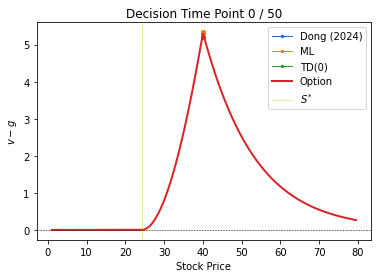
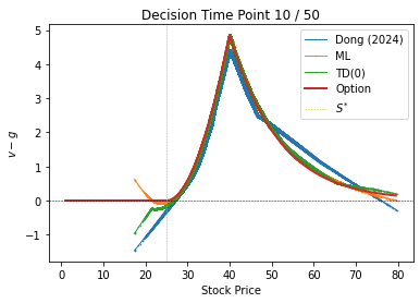
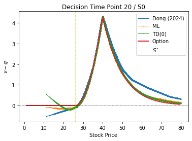
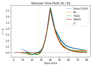
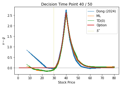
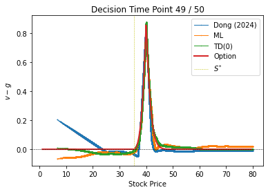
Figure 1: Learning results of $v-g$ under the TD algorithm in Dong, (2024), the offline ML algorithm and the online TD(0) algorithm in this paper at six selected decision time points: $\{0,10,20,30,40,49\}$-th discretized time points. The solid red lines are the theoretical values of $v-g$ and the dotted yellow vertical lines specify the stock price on the theoretical free boundary, both derived by finite difference. The training parameters of Dong (2024) are specified in Section 4.6.

As observed, all the algorithms result in values close to the oracle value, especially when the stock price is above $S^{*}$. The results of Dong, (2024) have relatively high errors when approaching the terminal time, which is the main motivation for learning early exercise premium instead in this paper. Except for extremely low stock prices, which are rarely reached by our simulated stock price trajectories leading to too few data for adequate learning, the yellow dotted vertical lines well separate the positive values from the non-positive ones. This result is desired when we construct the execution policy in the next subsection.

4.3 Execution policy

After having learned the exploratory value functions with well-trained NNs, we can further obtain the stopping probabilities by (2.23). However, when it comes to real execution regarding stopping or continuing, it does not seem reasonable to actually toss a biased coin. To wit, randomization is necessary for training, but not for execution. For the latter, one way is to use the mean of the randomized control (Dai et al.,, 2023), which is, however, inapplicable in the current 0–1 optimal stopping context. For example, a mean of 0.8 is outside of the control value set $\{0,1\}$.

Recall that for the classical (non-RL) optimal stopping problem of the American put option, the stopping region is characterized by $\mathcal{S}=\left\{(t,x):v(t,x)=g(x)\right\}$ while the continuation region is characterized by $\mathcal{C}=\left\{(t,x):v(t,x)>g(x)\right\}$. Thus, it is reasonable to base the sign of $w_{\theta_{l}}=V_{\theta_{l}}-\tilde{g}^{\phi}$ in (4.4) to make an exercise decision at time $t_{l}$. Theoretically, by (2.23), when the penalty factor $K$ goes to infinity, $\pi^{*}$ tends to 1 and 0 when $w_{\theta_{l}}<0$ and $w_{\theta_{l}}>0$, respectively. However, $K$ is finite in our implementation, $\pi^{*}$ in (2.23) is more likely to be neither 0 nor 1; but 0.5 is an appropriate threshold to divide between $w_{\theta_{l}}<0$ and $w_{\theta_{l}}>0$. In Figure 2, we randomly choose 100 stock price trajectories from the testing dataset, and classify the learned stopping strategies into two groups based on either $\pi^{*}\geqslant 0.5$ or $\pi^{*}<0.5$. When the former occurs the agent chooses to exercise the option, which is represented by the green triangle; otherwise the agent does not exercise, represented by the red circle. Besides, the blue line corresponds to the free boundary of this American put option $X_{f}(t)$. As Figure 2 shows, after sufficient training, both algorithms effectively classify almost all the exercise/non-exercise time–price pairs.

Next, we calculate the accuracy rate of classification at each time point as

$$\frac{\#\left\{\text{correctly classified sample points}\right\}}{M_{\mathrm{test}}}.$$

It turns out that both algorithms achieve accuracy rates of higher than $95\%$ for all discretized time points.

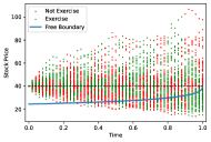
(a) Random initialization

(b) By ML with 1000 training steps

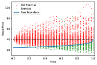
(c) By TD(0) with 5000 training steps

Figure 2: Stopping strategies learned from the two algorithms. The blue line is the theoretical free boundary of the American put option derived by finite difference. In each panel, there are 100 stock price trajectories with 50 discretized time points. The red circles correspond to the cases for which the stopping probability is less than half, while the green triangles to the cases for which the stopping probability is larger than or equal to half.

4.4 Option price

With the execution policy determined in Section 4.3, how to compute the option price? In this subsection, we introduce two ways to do it based on the learned exploratory value functions in Section 4.2.

The first way is to calculate the value of the original optimal stopping problem with the stopping time determined by the learned exploratory value functions in Section 4.2, namely

$$\mathcal{P}_{\mathrm{stopping}}:=\mathbb{E}\left[e^{-\rho\tau}g(X_{\tau})\right],$$ (4.5)

where

$$\tau:=\inf\left\{t_{l}:V_{\theta_{l}}(X_{t_{l}})\leqslant\tilde{g}^{\phi}(t_{l},X_{t_{l}}),\ l\in\left\{0,1,...,L\right\}\right\}\wedge T$$ (4.6)

with the convention that the infimum of an empty set is infinity.

The second way is to calculate the value (2.11) at the initial state $s=0,x=x_{0}$ under the execution policy determined in Section 4.3, namely

$$\mathcal{P}_{\mathrm{control}}:=\operatorname{\mathbb{E}}\!\left[\int_{s}^{T}Ke^{-K\int_{s}^{t}u_{r}\operatorname{d}\!r}g(t,X_{t})u_{t}\operatorname{d}\!t+e^{-K\int_{s}^{T}u_{r}\operatorname{d}\!r}g(T,X_{T})\;\bigg{|}\;X_{s}=x\right],$$ (4.7)

where

$$u(t,x)=1\mbox{ if }V_{\theta_{l}}(x)\leqslant\tilde{g}^{\phi}(t,x),\mbox{ and 0 otherwise, for $(t,x)\in[0,T)\times\mathbb{R}$.}$$ (4.8)

The relative error is defined as $\frac{|\mathcal{P}-5.317|}{5.317}$. We calculate the relative error on the testing dataset every 10 training steps. The learning curves of option price from the two methods described above are plotted in Figure 3.

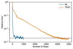
(a) $\mathcal{P}_{\mathrm{stopping}}$

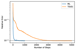
(b) $\mathcal{P}_{\mathrm{control}}$

Figure 3: Learning curves of option price $\mathcal{P}_{\mathrm{stopping}}$ defined in (4.5) and $\mathcal{P}_{\mathrm{control}}$ defined in (4.7) by offline ML (blue line) and online TD(0) (orange line) algorithms. We train the ML algorithm for 1000 steps and TD(0) algorithm for 5000 steps. Values of model parameters used for training are specified in Table 1.

First, we find that the ML algorithm has faster convergence than the online TD(0). This is because the latter needs to update parameters at every small time steps. Second, both algorithms eventually achieve very low relative errors (about $0.2\%$ and $1\%$ on average for $\mathcal{P}_{\mathrm{stopping}}$ and $\mathcal{P}_{\mathrm{control}}$, respectively). Thus, the RL algorithms prove to be effective in terms of learning the option price without knowing the true value of the volatility $\sigma$.

We observe that the relative errors in the second method converge to the level about $1\%$. This is due to the finite value of the penalty factor $K=10$ chosen in Table 1. In the next subsection, we will show that as $K$ increases, the relative error can be further reduced.

4.5 Sensitivity analysis

In this subsection, we carry out a sensitivity analysis on the impacts of the values of the penalty factor $K$ and the temperature parameter $\lambda$ on learning.

4.5.1 Penalty factor

We examine the effect of penalty factor on the learned option price in this subsection. First, it follows from (3.6) that $0<K\leqslant\frac{1}{\Delta t}=50$ in our setting. We pick $K\in\left\{1,5,10,20,30,40,50\right\}$ and keep the other model parameter values unchanged as in Table 1. Figure 4 shows the learning curves of option prices with a combination of the two algorithms and the two alternative ways. As expected, the higher the value of $K$, the less the relative error achieved by both algorithms. However, when $K$ increases to a certain level, a further increase no longer helps decrease the error, in which case the sampling error dominates.

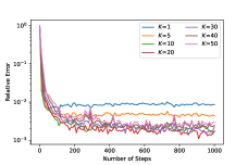
(a) $\mathcal{P}_{\mathrm{stopping}}$ by ML

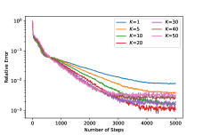
(b) $\mathcal{P}_{\mathrm{stopping}}$ by TD(0)

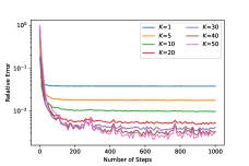
(c) $\mathcal{P}_{\mathrm{control}}$ by ML

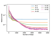
(d) $\mathcal{P}_{\mathrm{control}}$ by TD(0)

Figure 4: Learning curves of option prices $\mathcal{P}_{\mathrm{stopping}}$ defined in (4.5) and $\mathcal{P}_{\mathrm{control}}$ defined in (4.7) by offline ML and online TD(0) algorithms. In each panel, the penalty factor $K$ takes value from the set $\{1,5,10,20,30,40,50\}$ while other parameter values are set in Table 1. We train the ML algorithm for 1000 steps and TD(0) algorithm for 5000 steps. In all cases, the relative errors decrease in $K$.

4.5.2 Temperature parameter

The temperature parameter controls the weight on exploration, and thus is important for learning. Figure 5 shows the learning curves of option prices when $\lambda\in\left\{0.1,0.5,1,3,5,10\right\}$, while keeping the other model parameter values as in Table 1. We observe that in general, the smaller the temperature parameter, the more accurate but the lower the learning speed for convergence, which is especially evident in the TD(0) case. An implication of this observation is that if the computing resource is limited so the number of training steps is small, we can increase $\lambda$ to accelerate convergence. Intriguingly, in Figure 5, the errors are not monotonic in $\lambda$ when $\lambda\leqslant 1$ in the two cases using $\mathcal{P}_{\mathrm{stopping}}$. We conjecture that it is because the effect of $\lambda$ is dominated by the sampling error when $\lambda$ is sufficiently small. However, overall, the differences are around $0.3\%$ for $\lambda\in\{0.1,0.5,1\}$, which are sufficiently small.

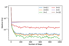
(a) $\mathcal{P}_{\mathrm{stopping}}$ by ML

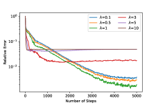
(b) $\mathcal{P}_{\mathrm{stopping}}$ by TD(0)

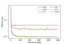
(c) $\mathcal{P}_{\mathrm{control}}$ by ML

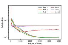
(d) $\mathcal{P}_{\mathrm{control}}$ by TD(0)

Figure 5: Learning curves of $\mathcal{P}_{\mathrm{stopping}}$ defined in (4.5) and $\mathcal{P}_{\mathrm{control}}$ defined in (4.7) by offline ML and online TD(0) algorithms. In each panel, the penalty factor $K$ is fixed to 10 and the temperature parameter $\lambda$ takes value from the set $\{0.1,0.5,1,3,5,10\}$ while other parameter values are chosen by Table 1. We train the ML algorithm for 1000 steps and TD(0) algorithm for 5000 steps.

4.6 Comparison with Dong (2024)

Both Dong, (2024) and this paper study RL for optimal stopping, but there are considerable differences as discussed in the introduction section. In particular, there is a considerable technical difference in terms of the entropy terms introduced in the respective RL objectives. It turns out that, when formulated in our setting with the penalty factor $K$, the decision variable $\tilde{\pi}$ in Dong, (2024) is the product of $K$ and the probability of stopping in our paper, i.e., $\tilde{\pi}=K\pi$. The entropy used in Dong, (2024) is $R(\tilde{\pi}):=\tilde{\pi}-\tilde{\pi}\log\tilde{\pi}=R(K\pi)=K\pi-K\pi\log(K\pi),$ whereas we take the differential entropy $-\mathscr{H}(\pi)=-\pi\log\pi-(1-\pi)\log(1-\pi).$ Dong, (2024) explains that $R(\tilde{\pi})$ is proposed by assuming $\tilde{\pi}\Delta t$ to be the probability of stopping in a $\Delta t$-length time interval and then integrating the differential entropy $-\mathscr{H}(\tilde{\pi}\Delta t)=-\tilde{\pi}\Delta t\log\Delta t+\left(\tilde{\pi}-\tilde{\pi}\log\tilde{\pi}\right)\Delta t+o(\Delta t)$ over the whole time horizon while dropping the first divergence term. In other words, it is not the exact differential entropy of the randomized strategy as in our paper.

Next, we compare the performances of the algorithms between the two papers. We use $\mathcal{P}_{\mathrm{stopping}}$ defined in (4.5) for computing option price, as it is the one taken by Dong, (2024). For a fair comparison, we use the TD error employed in Dong, (2024) as the criterion for performance and we learn the option price instead of the early exercise premium. We implement training for 1000 steps for both algorithms and repeat the training for 10 times. Because the scales of the entropy terms used in the two papers are considerably different, we train the two algorithms for different combinations of temperature parameter $\lambda\in\left\{10,1,0.1,0.01,0.001,0.0001\right\}$ and learning rate $\alpha\in\left\{0.1,0.01,0.001,0.0001\right\}$. The other parameters are kept the same as in Table 1 and the simulated stock price samples are the same for both algorithms. We then check the learning speeds of the two algorithms. Since the theoretical option price is 5.317, we examine the learning speeds for all the cases of $(\lambda,\alpha)$ in which the learned option prices are at least 5.29 for a meaningful comparison. We find that our algorithm is always faster than Dong, (2024)’s. Figure 6 is an illustration with $(\lambda,\alpha)=(0.001,0.01)$ (these are the model parameters corresponding to the solid blue line in Figure 1) in Dong’s algorithm and $(\lambda,\alpha)=(1,0.1)$ in our algorithm. The figure shows that both algorithms achieve very low relative errors ($0.39\%$ for our method and $0.44\%$ for Dong’s method) after 1000 training steps, but our algorithm is around 200 steps faster in convergence. One of the reasons may be that compared to the differential entropy in our algorithm, the scale of the entropy term in Dong, (2024) is larger, causing more biases in learning the objective stopping value.

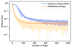
Figure 6: Learning curves of option price from our algorithm and Dong, (2024)’s. We repeat the training for 10 times to calculate the standard deviations of the learned option prices, which are represented as the shaded areas. The width of each shaded area is twice the corresponding standard deviation. Note that the vertical axis uses a logarithmic scale.

The simulation study reported so far is for an American option, whose price is evaluated under the risk-neutral probability. However, the underlying stock price is in general not observable in the risk-neural world; hence pricing American options is not the best example for illustrating a data-driven approach such as RL. Here, we present another application to demonstrate the effectiveness of our method in which the physical probability measure instead of the risk-neutral one is used (and thus all the relevant data are observable). Specifically, Dai and Dong, (2024) consider the problem of learning an optimal investment policy to maximize a portfolio’s terminal log return in the presence of proportional transaction costs, and turn it into an equivalent Dynkin game which involves optimal stopping decisions of two players. The latter is naturally formulated under the physical measure, and suitable for RL study under the frameworks of both Dong, (2024) and this paper; refer to Appendix D for RL for details. Dai and Dong, (2024) extend the RL algorithm of Dong, (2024) to learn an optimal investment policiy with transaction costs. With the same model parameters as in Dai and Dong, (2024) and a penalty factor $K=5$ (which is a proper choice when the time horizon is equally divided into 10 time intervals and there exist two stopping times in the Dynkin game), we learn how to trade in the Black–Scholes market under the penalty formulation, and compare the learning results of free boundaries and average log return when applying the learned strategies in a 20-year horizon. Similar to the case of the American put option, we choose temperature parameter $\lambda\in\left\{10^{-2},10^{-4},10^{-6}\right\}$ and learning rate $\alpha\in\left\{0.1,0.05,0.01,0.005\right\}$, and keep the other training parameters and structures of neural networks the same as in Dai and Dong, (2024), with 15000 training steps for both algorithms. As noted, in this example the stock price samples are simulated under the physical measure. Our experiments show that among the 12 combinations of $\lambda$ and $\alpha$, Dai and Dong, (2024)’s algorithm achieves higher average log return in the last training step than our algorithm for 2 times, while we achieve better results for 10 times. For comparing the learning speeds, note that the omniscient level of average log return in the 20-year horizon under the testing dataset is around 3.00; so we choose the cases of $(\lambda,\alpha)$ in which the two algorithms achieve average log return values of greater than 2.95. We find that $(\lambda,\alpha)=(10^{-6},0.05)$ and $(\lambda,\alpha)=(10^{-2},0.01)$ result in the fastest convergence of average log return for Dai and Dong, (2024)’s algorithm and ours, respectively. Figure 7 plots the corresponding learning curves of the initial free boundaries and average log returns. Figure 7(a) shows that the convergence of the sell boundary is almost identical for the two algorithms, while the convergence of the buy boundary is faster under our algorithm. Figure 7(b) indicates that the convergence of average log return is around 5000 steps faster under our algorithm. It is interesting to note that the trivial buy-and-hold strategy leads to an average log return value of 2.5; so both the RL algorithms indeed help the agent “beat the market”.

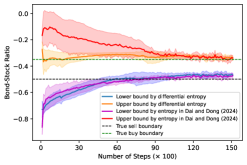
(a) Free boundaries at the initial time

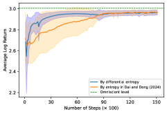
(b) Log return

Figure 7: Learning curves of free boundaries and average log return from our algorithm and Dai and Dong, (2024)’s. We repeat the training for 10 times to calculate the standard deviations of the learned free boundaries and average log return, which are represented as the shaded areas. The width of each shaded area is twice the corresponding standard deviation.

5 Conclusions

In this paper, we study optimal stopping for diffusion processes in the exploratory RL framework of Wang et al., (2020). Different from Dong, (2024) and Dai and Dong, (2024) which directly randomize stopping times for exploration through mixed strategies characterized by Cox processes, we turn the problem into stochastic control by approximating the variational inequalities with the so-called penalized PDE. This enables us to apply all the available results and methods developed recently in RL for controlled diffusion processes (Jia and Zhou, 2022a, ; Jia and Zhou, 2022b, ; Jia and Zhou,, 2023). Our simulation study shows that the resulting RL algorithms achieve comparable, and sometimes better, performance in terms of accuracy and speed than those in Dong, (2024) and Dai and Dong, (2024).

We take option pricing as an application of the general theory in our experiments. There is a caveat in this: the expectation in the pricing formula is with respect to the risk-neutral probability under which data are not observable. While we can use simulation to test the learning efficiency of an RL algorithm, for real applications we need to take a formulation for option pricing that is under the physical measure due to the data-driven nature of RL. One example of such a formulation is the mean–variance hedging.

There are many interesting problems to investigate along the lines of this paper, including convergence and regret analysis, choice of the temperature parameter, and more complex underlying processes to stop.

Appendix A Proofs of statements

A.1 Proof of Lemma 2.1

Suppose there is a positive sequence $\{K_{n}\}_{n\geqslant 1}$ that increases to infinity, and $v^{(n)}$ solves (2.5) with $K=K_{n}$. Denote by $a_{n}=v_{t}^{(n)}+\mathscr{L}v^{(n)},\ b_{n}=g-v^{(n)}$, $a_{\infty}=v_{t}+\mathscr{L}v$, and $b_{\infty}=g-v$, where $v$ is the limit of $v^{(n)}$. From (2.5) we have $a_{n}=-K_{n}(b_{n})^{+}\leqslant 0$. Because $\left(a_{n},b_{n}\right)$ converges to $\left(a_{\infty},b_{\infty}\right)$ as $n\rightarrow\infty$, we get $a_{\infty}\leqslant 0$. On the other hand, on any compact region, $\{a_{n}\}_{n\geqslant 1}$ is locally bounded; so $(b_{n})^{+}=-\frac{a_{n}}{K_{n}}\rightarrow 0,\text{as $n\rightarrow\infty$}$, yielding $b_{\infty}\leqslant 0$.

If $b_{\infty}<0$, then there exists a large number $N$ such that $b_{n}<0$ for all $n>N$, leading to $a_{n}=0$ for all $n>N$. Thus, $a_{\infty}=0$ when $b_{\infty}<0$.

Hence, we have $a_{\infty}\leqslant 0$, $b_{\infty}\leqslant 0$ and $a_{\infty}b_{\infty}=0$, which implies that $v$ solves (2.3).

A.2 Proof of Theorem 2.2

For notational simplicity, we only consider the case when $X$ and $W$ are both one-dimensional.

Write $\overline{R}_{t}=e^{-\int_{s}^{t}f(r,X_{r},u_{r})\operatorname{d}\!r},\ t\geqslant s$. Then $\operatorname{d}\!\overline{R}_{t}=-\overline{R}_{t}f(t,X_{t},u_{t})\operatorname{d}\!t,\ \overline{R}_{s}=1$. Itô’s lemma gives

$$\quad\;\operatorname{d}\!\;(\overline{R}_{t}v(t,X_{t}))$$

$$=\overline{R}_{t}\operatorname{d}\!v(t,X_{t})+v(t,X_{t})\operatorname{d}\!\overline{R}_{t}$$

$$=\overline{R}_{t}\big{[}\left(v_{t}(t,X_{t})+\mathscr{L}_{u}v(t,X_{t})\right)\operatorname{d}\!t+v_{x}(t,X_{t})\sigma(t,X_{t},u_{t})\operatorname{d}\!W_{t}\big{]}-v(t,X_{t})\overline{R}_{t}f(t,X_{t},u_{t})\operatorname{d}\!t$$

$$=\overline{R}_{t}\big{[}\left(v_{t}(t,X_{t})+\mathscr{L}_{u}v(t,X_{t})-v(t,X_{t})f(t,X_{t},u_{t})\right)\operatorname{d}\!t+v_{x}(t,X_{t})\sigma(t,X_{t},u_{t})\operatorname{d}\!W_{t}\big{]}$$

$$\leqslant-\overline{R}_{t}G(t,X_{t},u_{t})\operatorname{d}\!t+\overline{R}_{t}v_{x}(t,X_{t})\sigma(t,X_{t},u_{t})\operatorname{d}\!W_{t},$$

where the last inequality is due to (2.9) and $\overline{R}_{t}>0$. Integrating both sides from $s$ to $T$ and then taking conditional expectation yield

$$\operatorname{\mathbb{E}}\!\left[\overline{R}_{T}v(T,X_{T})-\overline{R}_{s}v(s,X_{s})\;\big{|}\;X_{s}=x\right]\leqslant-\operatorname{\mathbb{E}}\!\left[\int_{s}^{T}\overline{R}_{t}G(t,X_{t},u_{t})\operatorname{d}\!t\;\bigg{|}\;X_{s}=x\right].$$

As $\overline{R}_{s}=1$, the above leads to

$$v(s,x) \geqslant\operatorname{\mathbb{E}}\!\left[\int_{s}^{T}\overline{R}_{t}G(t,X_{t},u_{t})\operatorname{d}\!t+\overline{R}_{T}v(T,X_{T})\;\bigg{|}\;X_{s}=x\right]$$

$$=\operatorname{\mathbb{E}}\!\left[\int_{s}^{T}e^{-\int_{s}^{t}f(r,X_{r},u_{r})\operatorname{d}\!r}G(t,X_{t},u_{t})\operatorname{d}\!t+e^{-\int_{s}^{T}f(r,X_{r},u_{r})\operatorname{d}\!r}H(X_{T})\;\bigg{|}\;X_{s}=x\right].$$

This means that $v$ is an upper bound of the value function of problem (2.7). All the inequalities above become equalities if we take $u\in U$ that solves the optimization problem in (2.9). Therefore, we conclude $v$ is the value function of (2.7).

A.3 Proof of Theorem 3.1

By the Feynman–Kac formula, for any $(t,x)$,

$$\partial_{t}J^{\pi}(t,x)+\mathscr{L}J^{\pi}(t,x)+H\left(t,x,\pi,J^{\pi}\right)=0,$$

where

$$H\left(t,x,\pi,J^{\pi}\right):=K\pi(t,x)\left(g(t,x)-J^{\pi}(t,x)\right)-\lambda\mathscr{H}(\pi(t,x)).$$

Similarly, for any $(t,x)$,

$$\partial_{t}J^{\tilde{\pi}}(t,x)+\mathscr{L}J^{\tilde{\pi}}(t,x)+H\left(t,x,\tilde{\pi},J^{\tilde{\pi}}\right)=0,$$

where $\tilde{\pi}$ is defined in (3.1). It turns out that

$$\tilde{\pi}(t,x)=\operatorname*{argmax}_{\pi\in[0,1]}H\left(t,x,\pi,J^{\pi}\right).$$

Denote $\Delta(t,x):=J^{\tilde{\pi}}(t,x)-J^{\pi}(t,x)$. Then

$$\partial_{t}\Delta(t,x)+\mathscr{L}\Delta(t,x)+H\left(t,x,\tilde{\pi},J^{\tilde{\pi}}\right)-H\left(t,x,\pi,J^{\pi}\right)=0.$$

Because

$$H\left(t,x,\tilde{\pi},J^{\tilde{\pi}}\right)-H\left(t,x,\pi,J^{\pi}\right)$$

$$= \ H\left(t,x,\tilde{\pi},J^{\tilde{\pi}}\right)-H\left(t,x,\tilde{\pi},J^{\pi}\right)+H\left(t,x,\tilde{\pi},J^{\pi}\right)-H\left(t,x,\pi,J^{\pi}\right)$$

$$= -K\tilde{\pi}(t,x)\Delta(t,x)+H\left(t,x,\tilde{\pi},J^{\pi}\right)-H\left(t,x,\pi,J^{\pi}\right),$$

we have

$$\partial_{t}\Delta(t,x)+\mathscr{L}\Delta(t,x)-K\tilde{\pi}(t,x)\Delta(t,x)=H\left(t,x,\pi,J^{\pi}\right)-H\left(t,x,\tilde{\pi},J^{\pi}\right)\leqslant 0,$$

where the last inequality is from the definition of $\tilde{\pi}$. Besides, $\Delta(T,x)=0$ at the terminal time $T$. Therefore, 0 is a sub-solution of $-\partial_{t}u(t,x)-\mathscr{L}u(t,x)+K\tilde{\pi}(t,x)u(t,x)+H\left(t,x,\pi,J^{\pi}\right)-H\left(t,x,\tilde{\pi},J^{\pi}\right)=0$. By the maximum principle, we have $\Delta(t,x)\geqslant 0$, resulting in $J^{\tilde{\pi}}(t,x)\geqslant J^{\pi}(t,x)$.

Appendix B Learning early exercise premium

In this section, we discuss how to learn the early exercise premium of an American put option.

Recall we have an explicit pricing formula for a European put option:

$$\begin{cases}V_{E}(t,x)=\Gamma e^{-\rho(T-t)}N\left(-d_{-}(t,x)\right)-xN\left(-d_{+}(t,x)\right),\ t\in[0,T),\\ V_{E}(T,x)=g(x),\end{cases}$$ (B.1)

where $d_{\pm}(t,x)=\frac{1}{\sigma\sqrt{T-t}}\left[\log\left(\frac{x}{\Gamma}\right)+\left(\rho\pm\frac{1}{2}\sigma^{2}\right)\left(T-t\right)\right]$, and $N(\cdot)$ is the cumulative standard normal distribution function $N(y)=\frac{1}{\sqrt{2\pi}}\int_{-\infty}^{y}e^{-\frac{z^{2}}{2}}dz=\frac{1}{\sqrt{2\pi}}\int_{-y}^{\infty}e^{-\frac{z^{2}}{2}}dz$.

The early exercise premium of the American put option is

$$\tilde{v}(t,x):=v(t,x)-V_{E}(t,x),$$ (B.2)

where $v(t,x)$ is the option value at the time–state pair $(t,x)$. The associated payoff function is

$$\tilde{g}(t,x):=g(x)-V_{E}(t,x).$$ (B.3)

By (2.3) and the fact that $V_{E}$ satisfies $\frac{\partial}{\partial t}V_{E}+\mathscr{L}V_{E}=0$ with terminal condition $V_{E}(T,x)=g(x)$, we have

$$\begin{cases}\max\{\tilde{v}_{t}+\mathscr{L}\tilde{v},\ \tilde{g}-\tilde{v}\}=0,\ (t,x)\in[0,T)\times\operatorname{\mathbb{R}},\\ \tilde{v}(T,x)=0.\end{cases}$$ (B.4)

Thus, the terminal condition is smooth now, and the related PDE by penalty approximation is

$$\begin{cases}\tilde{v}_{t}+\max_{u\in\{0,1\}}\left\{\mathscr{L}\tilde{v}-Ku\tilde{v}+K\tilde{g}(t,x)u\right\}=0,\ (t,x)\in[0,T)\times\operatorname{\mathbb{R}},\\ \tilde{v}(T,x)=0.\end{cases}$$

Consequently, by Theorem 2.2 the corresponding control problem is

$$\max_{u\in\{0,1\}}\;\operatorname{\mathbb{E}}\!\left[\int_{s}^{T}Ke^{-K\int_{s}^{t}u_{r}\operatorname{d}\!r}\tilde{g}(t,X_{t})u_{t}\operatorname{d}\!t\;\bigg{|}\;X_{s}=x\right],$$ (B.5)

and the entropy-regularized exploratory problem is

$$\max_{\pi\in[0,1]}\;\operatorname{\mathbb{E}}\!\left[\int_{s}^{T}e^{-K\int_{s}^{t}\pi_{v}\operatorname{d}\!v}\big{[}K\tilde{g}(t,X_{t})\pi_{t}-\lambda\mathscr{H}(\pi_{t})\big{]}\operatorname{d}\!t\;\bigg{|}\;X_{s}=x\right].$$ (B.6)

While we could use the algorithms in Section 3 to learn $\tilde{v}$, $\tilde{g}$ is not fully known to us since $\sigma$ (which appears in $V_{E}$) is an unknown model parameter.

To deal with the unknown payoff function $\tilde{g}$, recall

$$\tilde{g}(t,x)=g(x)-V_{E}(t,x)=\left(\Gamma-x\right)^{+}-V_{E}(t,x).$$ (B.7)

Hence, in the formula of $V_{E}$, namely (B.1), we replace $\sigma$ by $\phi$, which is a parameter to learn with a properly chosen initial value. Denote by $V_{E}^{\phi}$ and $\tilde{g}^{\phi}$ the parameterized European option value function and payoff function, respectively. Note that

$$V_{E}(t,x)=\mathbb{E}\left[e^{-\rho(T-t)}g(X_{T})\;\bigg{|}\;X_{t}=x\right]=\mathbb{E}\left[e^{-\rho(T-t)}\left(\Gamma-X_{T}\right)^{+}\;\bigg{|}\;X_{t}=x\right].$$ (B.8)

This is a policy evaluation problem. Thanks to the martingale approach developed in Jia and Zhou, 2022a , we can learn/update $\phi$ by minimizing the martingale loss w.r.t. $\phi$:

$$\quad\quad\text{ML}\left(\phi\right) \approx\frac{1}{2}\mathbb{E}\left[\sum_{l=0}^{L-1}\left(e^{-\rho T}V_{E}\left(T,X_{T}\right)-e^{-\rho t}V_{E}^{\phi}\left(t_{l},X_{l}\right)\right)^{2}\Delta t\right]$$ (B.9)

$$=\frac{1}{2}\mathbb{E}\left[\sum_{l=0}^{L-1}\left(e^{-\rho T}\left(\Gamma-X_{T}\right)^{+}-e^{-\rho t}V_{E}^{\phi}\left(t_{l},X_{l}\right)\right)^{2}\Delta t\right].$$

In each episode, we simulate a batch of stock price trajectories and then use the stochastic gradient descent method to minimize the above loss function to update $\phi$. Figure 8 shows the efficacy of this policy evaluation algorithm, with an initial guess of the unknown $\sigma$ to be 0.8, twice the true value.

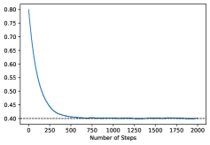
Figure 8: Learning curve of $\phi$, which is used to parameterize the payoff function (B.7) by minimizing the martingale loss (B.9). The initialization of $\phi$ is 0.8, and the true value of $\sigma$ is 0.4. The value of $\phi$ after 2000 steps is 0.4006.

We emphasize that in this particular example of European option, due to the availability of the explicit formula of the option price, the critic parameter $\phi$ happens to be a model parameter $\sigma$. In general, for more complicated problems with little structure, the actor/critic parameters may be very different from the model primitives and may themselves have no physical/practical meanings at all. Estimating model parameters is not a goal of RL in our framework.

Appendix C Additional results for sensitivity tests

In Figure 9, we show a sensitivity test when the penalty factor approaches its maximum possible value, i.e., $K=50$, under our time discretization setting. In this case, the two ways of calculating the option price have almost the same results, which is consistent with Lemma 2.1. The trade-off between learning accuracy and speed observed previously still holds.

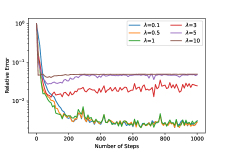
(a) $\mathcal{P}_{\mathrm{stopping}}$ by ML

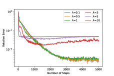
(b) $\mathcal{P}_{\mathrm{stopping}}$ by TD(0)

(c) $\mathcal{P}_{\mathrm{control}}$ by ML

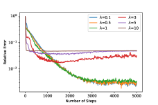
(d) $\mathcal{P}_{\mathrm{control}}$ by TD(0)

Figure 9: Learning curves of option prices $\mathcal{P}_{\mathrm{stopping}}$ defined in (4.5) and $\mathcal{P}_{\mathrm{control}}$ defined in (4.7) by offline ML and online TD(0) algorithms. In each panel, the penalty factor $K$ is fixed to 50 and the temperature parameter $\lambda$ takes value from the set $\{0.1,0.5,1,3,5,10\}$ while the other parameter values are set as in Table 1. We train the ML algorithm for 1000 steps and TD(0) algorithm for 5000 steps.

Appendix D RL for Dynkin games

Theorem 1 in Dai and Dong, (2024) reveals that Merton’s problem with proportional transaction costs is equivalent to a Dynkin game that is essentially an optimal stopping problem. Here, we focus on the Black–Scholes market where the stock price follows

$$\operatorname{d}\!S_{t}=\alpha S_{t}\operatorname{d}\!t+\sigma S_{t}\operatorname{d}\!W_{t},$$

where $\alpha$ and $\sigma$ are constants but unknown to the agent. The value function of the Dynkin game satisfies the following variational inequalities

$$\max\left\{\min\left\{-w_{t}-\mathcal{L}w,w-L(x)\right\},w-U(x)\right\}=0$$ (D.1)

with terminal condition

$$w(T,x)=\frac{x}{x+1-\theta},$$ (D.2)

where $\theta\in(0,1)$ is the proportional transaction cost rate, $x$ is the bond–stock position ratio, $\mathcal{L}$ is the generator of this ratio process, and $L(x)$ and $U(x)$ are respectively the lower and upper obstacles of $w(t,x)$.

It is proved in Zhang et al., (2022) that (D.1) can be approximated by the following penalized PDE:

$$-w_{t}-\mathcal{L}w-K\left(w-L(x)\right)^{-}+K\left(w-U(x)\right)^{+}=0,$$ (D.3)

where $K>0$ is a large penalty factor. This PDE can be equivalently written as

$$w_{t}+\max_{a\in\left\{0,1\right\}}\min_{b\in\left\{0,1\right\}}\left\{\mathcal{L}w-wf(t,x,a,b)+G(t,x,a,b)\right\}=0,$$ (D.4)

where

$$f(t,x,a,b)=K(a+b),\quad G(t,x,a,b)=K\left(L(x)a+U(x)b\right).$$

Similar to the setup in Section 2.2, we consider a constrained differential game:

$$w(s,x)=\max_{a\in\mathscr{U}}\min_{b\in\mathscr{U}}J(s,x;a,b),$$ (D.5)

where

$$J(s,x;a,b)=\mathbb{E}\Bigg{[}\int_{s}^{T} e^{-\int_{s}^{t}f(r,X_{r},a_{r},b_{r})\operatorname{d}\!r}G(t,X_{t},a_{t},b_{t})\operatorname{d}\!t$$

$$+e^{-\int_{s}^{T}f(r,X_{r},a_{r},b_{r})\operatorname{d}\!r}H(X_{T})\;\bigg{|}\;X_{s}=x\Bigg{]},$$

and the controlled $n$-dimensional process $X$ follows

$$\operatorname{d}\!X_{t}=b(t,X_{t},a_{t},b_{t})\operatorname{d}\!t+\sigma(t,X_{t},a_{t},b_{t})\operatorname{d}\!W_{t}.$$ (D.6)

We have the following result.

Theorem D.1 (Verification theorem).

Suppose $w$ is a classical solution of

$$\begin{cases}w_{t}+\max_{a\in U}\min_{b\in U}\left\{\mathscr{L}_{a,b}w-wf+G\right\}=0,~{}~{}(t,x)\in[0,T)\times\operatorname{\mathbb{R}}^{n},\\ w(T,x)=H(x),\end{cases}$$ (D.7)

where

$$\mathscr{L}_{a,b}w=\frac{1}{2}\sum_{i,j,k}\sigma_{i,k}(t,x,a,b)\sigma_{j,k}(t,x,a,b)\frac{\partial^{2}w}{\partial x_{i}\partial x_{j}}+\sum_{i}b_{i}(t,x,a,b)\frac{\partial w}{\partial x_{i}}.$$

Then it is the value function of problem (D.5).

Proof.

Let $\overline{R}_{t}=e^{-\int_{s}^{t}f(r,X_{r},a_{r},b_{r})\operatorname{d}\!r},\ t\geqslant s$. Then $\operatorname{d}\!\overline{R}_{t}=-\overline{R}_{t}f(t,X_{t},a_{t},b_{t})\operatorname{d}\!t$ and $\overline{R}_{s}=1.$

For each fixed ${a\in U}$, let $b^{*}_{t}=b_{t}^{*}(x,a)$ denote the minimizer of $\mathscr{L}_{a,b}w-wf+G$. By (D.7),

$$w_{t}+\max_{a\in U}\left\{\mathscr{L}_{a,b^{*}}w-wf(t,x,a,b^{*})+G(t,x,a,b^{*})\right\}=0.$$

Then, similar to the proof in Appendix A.2, we get for any admissible process $a\in\mathscr{U}$,

$$w(s,x) \geqslant\operatorname{\mathbb{E}}\!\left[\int_{s}^{T}\overline{R}_{t}^{a,b^{*}}G(t,X_{t},a_{t},b_{t}^{*})\operatorname{d}\!t+\overline{R}_{T}^{a,b^{*}}w(T,X_{T})\;\bigg{|}\;X_{s}=x\right]$$

$$=\operatorname{\mathbb{E}}\!\left[\int_{s}^{T}e^{-\int_{s}^{t}f(r,X_{r},a_{r},b_{r}^{*})\operatorname{d}\!r}G(t,X_{t},a_{t},b_{t}^{*})\operatorname{d}\!t+e^{-\int_{s}^{T}f(r,X_{r},a_{r},b_{r}^{*})\operatorname{d}\!r}H(X_{T})\;\bigg{|}\;X_{s}=x\right]$$

$$=J(s,x;a,b^{*})$$

$$\geqslant\min_{b\in\mathscr{U}}J(s,x;a,b).$$

Since $a\in\mathscr{U}$ is arbitrarily chosen, the above implies

$$w(s,x)\geqslant\max_{a\in\mathscr{U}}\min_{b\in\mathscr{U}}J(s,x;a,b).$$

Hence, $w$ is an upper bound of the value function of problem (D.5).

On the other hand, if we choose a pair $(a^{*},b^{*}_{t}(x,a^{*}))$ to solve

$$\max_{a\in U}\min_{b\in U}\left\{\mathscr{L}_{a,b}w-wf+G\right\},$$

all the inequalities in the above become equalities, yielding that $w$ is the value function of (D.5).

Following the same procedure as in Section 2.2, we find that the solution to (D.4) satisfying the terminal condition is the value function of the following stochastic differential game (Fleming and Soner,, 2006):

$$w(s,x)=\max_{a_{t}\in\{0,1\}}\min_{b_{t}\in\{0,1\}}J(s,x;a,b),$$ (D.8)

where

$$J(s,x;a,b)=\mathbb{E}\Big{[}\int_{s}^{T} Ke^{-K\int_{s}^{t}(a_{r}+b_{r})\operatorname{d}\!r}\left(L(X_{t})a_{t}+U(X_{t})b_{t}\right)\operatorname{d}\!t$$

$$+e^{-K\int_{s}^{T}(a_{r}+b_{r})\operatorname{d}\!r}\frac{X_{T}}{X_{T}+1-\theta}\;\bigg{|}\;X_{s}=x\Big{]}.$$

Next, we randomize $\{a_{t}\}_{t\in[0,T]}$ and $\{b_{t}\}_{t\in[0,T]}$ respectively by $\{\nu_{t}\}_{t\in[0,T]}$ and $\{\mu_{t}\}_{t\in[0,T]}$, where

$$\nu_{t}=\mathbb{P}\left(a_{t}=1\right)=1-\mathbb{P}\left(a_{t}=0\right),\quad\mu_{t}=\mathbb{P}\left(b_{t}=1\right)=1-\mathbb{P}\left(b_{t}=0\right).$$

It turns out that the exploratory value function of the Dynkin game is

$$w^{\lambda}(s,x)=\max_{\nu_{t}\in[0,1]}\min_{\mu_{t}\in[0,1]}J^{\lambda}(s,x;\nu,\mu),$$ (D.9)

where

$$J^{\lambda}(s,x;\nu,\mu)=\mathbb{E}\Big{[}\int_{s}^{T} Ke^{-K\int_{s}^{t}(\nu_{r}+\mu_{r})\operatorname{d}\!r}\left[L(X_{t})\nu_{t}+U(X_{t})\mu_{t}-\lambda\left(\mathscr{H}(\nu_{t})-\mathscr{H}(\mu_{t})\right)\right]\operatorname{d}\!t$$

$$+e^{-K\int_{s}^{T}(\nu_{r}+\mu_{r})\operatorname{d}\!r}\frac{X_{T}}{X_{T}+1-\theta}\;\bigg{|}\;X_{s}=x\Big{]}.$$

The HJB equation of problem (D.9) is thus

$$w^{\lambda}_{t}+\mathcal{L}w^{\lambda}+\max_{\nu\in[0,1]}\min_{\mu\in[0,1]}\left\{-w^{\lambda}K(\nu+\mu)+K\left(L(x)\nu+U(x)\mu\right)-\lambda\left(\mathscr{H}(\nu)-\mathscr{H}(\mu)\right)\right\}=0,$$ (D.10)

and the optimal solutions are

$$\nu^{*} =\frac{\exp\left(\frac{K}{\lambda}(L(x)-w^{\lambda})\right)}{\exp\left(\frac{K}{\lambda}(L(x)-w^{\lambda})\right)+1}=\frac{1}{1+\exp\left(-\frac{K}{\lambda}(L(x)-w^{\lambda})\right)},$$ (D.11)

$$\mu^{*} =\frac{\exp\left(\frac{K}{\lambda}(w^{\lambda}-U(x))\right)}{\exp\left(\frac{K}{\lambda}(w^{\lambda}-U(x))\right)+1}=\frac{1}{1+\exp\left(-\frac{K}{\lambda}(w^{\lambda}-U(x))\right)}.$$

Consequently, if we choose the TD error criterion for policy evaluation, the RL algorithm is essentially the same as Algorithm 1 in Dai and Dong, (2024), except that $\nu,\mu,\nu^{*},\mu^{*}$ in their algorithm should be replaced by $K\nu,K\mu$, $\nu^{*},\mu^{*}$ in (D.11) in this section, and their entropy term should be replaced by the differential entropy in this paper.

Appendix E Finite difference method

In this section, we present (classical, model-based) algorithms for pricing a finite-horizon American put option and obtaining its stopping boundary. We use the penalty method in Forsyth and Vetzal, (2002). The payoff function is $g(x)=\left(\Gamma-x\right)^{+}$ with $x$ being the stock price and $\Gamma$ the strike price. We consider the PDE (2.5) and let $u(t,y):=v(t,x)$ with $x=e^{y}$. In the finite difference scheme below, the time horizon $\left[0,T\right]$ is divided to $N_{t}$ equally spaced intervals with $t_{i}=i\Delta t,\ \text{for }i=0,\ldots,N_{t}$, and the range for $y$ is chosen to be $\left[-N,N\right]$ with $N$ being a large positive number, which is further divided into $N_{y}$ equally spaced intervals with $y_{j}=-N+j\Delta y\ \text{for }j=0,\ldots,N_{y}$. Thus, $u_{i,j}$ denotes the numerical value at the mesh point $\left(t_{i},y_{j}\right)$, namely, $u_{i,j}:=u\left(t_{i},y_{j}\right)$ for $i=0,\ldots,N_{t},j=0,\ldots,N_{y}$.

In the following, let $u_{i,j}^{k}$ denotes the $k$-th iteration value of $u_{i,j}$. The terminal condition is

$$u_{N_{t},j}=g(e^{y_{j}})$$ (E.1)

for $j=0,\ldots,N_{y}$. Similarly, the boundary conditions at $y_{0}$ and $y_{N_{y}}$ are set to be

$$u_{i,0}=g(e^{y_{0}}),\ \text{and }u_{i,N_{y}}=g(e^{y_{N_{y}}})$$ (E.2)

for $i=0,\ldots,N_{t}$. The Black–Scholes operator $v_{t}(t,x)+\frac{1}{2}\sigma^{2}x^{2}v_{xx}(t,x)+\rho xv_{x}(t,x)-\rho v(t,x)$ changes to

$$\mathcal{L}_{BS}u(t,y):=u_{t}(t,y)+\frac{1}{2}\sigma^{2}u_{yy}(t,y)+\left(\rho-\frac{1}{2}\sigma^{2}\right)u_{y}(t,y)-\rho u(t,y).$$

By the fully implicit finite difference scheme,

$$\frac{\partial}{\partial t}u(t_{i},y_{j}) =\frac{u_{i+1,j}-u_{i,j}}{\Delta t},$$

$$\frac{\partial}{\partial y}u(t_{i},y_{j}) =\frac{u_{i,j+1}-u_{i,j-1}}{2\Delta y},$$

$$\frac{\partial^{2}}{\partial y^{2}}u(t_{i},y_{j}) =\frac{u_{i,j+1}-2u_{i,j}+u_{i,j-1}}{\left(\Delta y\right)^{2}},$$

for $j=1,\ldots,N_{y}-1$ and $i=0,\ldots,N_{t}-1$. The discretized Black–Scholes operator is therefore

$$\mathcal{L}_{BS}u_{i,j}=\frac{u_{i+1,j}-u_{i,j}}{\Delta t}+\beta u_{i,j+1}-\left(\alpha+\beta+\rho\right)u_{i,j}+\alpha u_{i,j-1},$$ (E.3)

where

$$\alpha=\frac{\sigma^{2}}{2\left(\Delta y\right)^{2}}-\frac{\rho-\frac{1}{2}\sigma^{2}}{2\Delta y},\ \text{and }\beta=\frac{\sigma^{2}}{2\left(\Delta y\right)^{2}}+\frac{\rho-\frac{1}{2}\sigma^{2}}{2\Delta y}.$$

The PDE in (2.5) becomes

$$-\mathcal{L}_{BS}u(t,y)=K\left(g(e^{y})-u(t,y)\right)^{+}.$$ (E.4)

For each mesh point $\left(t_{i},y_{j}\right)$, we use the following approximation by Newton iteration:

$$\left(g(e^{y_{j}})-u_{i,j}^{k+1}\right)^{+} =\left(g(e^{y_{j}})-u_{i,j}^{k}+u_{i,j}^{k}-u_{i,j}^{k+1}\right)^{+}$$

$$\approx\left(g(e^{y_{j}})-u_{i,j}^{k}\right)^{+}+1_{g(e^{y_{j}})-u_{i,j}^{k}>0}\left(u_{i,j}^{k}-u_{i,j}^{k+1}\right)$$

$$=\left(g(e^{y_{j}})-u_{i,j}^{k+1}\right)1_{g(e^{y_{j}})-u_{i,j}^{k}>0},$$ (E.5)

where $1_{A}$ is the indicator function of a set $A$. By (E.3) and (E), it turns out that (E.4) reads

$$-\frac{u_{i+1,j}-u_{i,j}^{k+1}}{\Delta t}-\beta u_{i,j+1}^{k+1}+\left(\alpha+\beta+\rho\right)u_{i,j}^{k+1}-\alpha u_{i,j-1}^{k+1}=K\left(g(e^{y_{j}})-u_{i,j}^{k+1}\right)1_{g(e^{y_{j}})-u_{i,j}^{k}>0},$$

which simplifies to

$$-\beta u_{i,j+1}^{k+1}+\left(\frac{1}{\Delta t}+\alpha+\beta+\rho+K1_{g(e^{y_{j}})-u_{i,j}^{k}>0}\right)u_{i,j}^{k+1}-\alpha u_{i,j-1}^{k+1}=\frac{u_{i+1,j}}{\Delta t}+Kg(e^{y_{j}})1_{g(e^{y_{j}})-u_{i,j}^{k}>0}.$$ (E.6)

In each iterative step, the quantities in the RHS of (E.6) regarding future values $u_{i+1,j}$ for all $j$ and previous estimates $u_{i,j}^{k}$ for all $i$ and $j$ are known, and the current estimates $u_{i,j}^{k+1}$ are obtained by solving the equation (E.6). See Algorithm 3 for details.

Inputs: $\Delta t,\Delta y,N,N_{t},N_{y},K$ and the tolerance level $\varepsilon>0$.

Learning procedure:

Initialize $u_{N_{t},j}$ for all $j$ by (E.1) as well as $u_{i,0}$ and $u_{i,N_{y}}$ for all $i$ by (E.2).

for $i=N_{t}-1,\ldots,0$ do

       Set $u_{i,j}^{0}=u_{i+1,j}$ for $j=1,\ldots,N_{y}-1$.

       for $k=0,1,\dots$ do

             Solve the equation (E.6) to get $u_{i,j}^{k+1}$ for $j=1,\ldots,N_{y}-1$.

             if ${||u_{i}^{k+1}-u_{i}^{k}||_{\infty}}<\varepsilon*{\max\left\{1,\ ||u_{i}^{k}||_{\infty}\right\}}$ then

                  Quit the loop for $k$.

             end if

            

       end for

      Set $u_{i,j}=u_{i,j}^{k+1}$ for $j=1,\ldots,N_{y}-1$.

      

end for

Algorithm 3 Finite difference scheme for (2.5)

References

• Barberis, (2012) Barberis, N. (2012). A model of casino gambling. Management Science, 58(1):35–51.
• Becker et al., (2019) Becker, S., Cheridito, P., and Jentzen, A. (2019). Deep optimal stopping. Journal of Machine Learning Research, 20(74):1–25.
• Becker et al., (2020) Becker, S., Cheridito, P., and Jentzen, A. (2020). Pricing and hedging American-style options with deep learning. Journal of Risk and Financial Management, 13(7):158.
• Becker et al., (2021) Becker, S., Cheridito, P., Jentzen, A., and Welti, T. (2021). Solving high-dimensional optimal stopping problems using deep learning. European Journal of Applied Mathematics, 32(3):470–514.
• Dai and Dong, (2024) Dai, M. and Dong, Y. (2024). Learning an optimal investment policy with transaction costs via a randomized Dynkin game. Available at SSRN 4871712.
• Dai et al., (2023) Dai, M., Dong, Y., and Jia, Y. (2023). Learning equilibrium mean-variance strategy. Mathematical Finance, 33(4):1166–1212.
• Dai et al., (2023) Dai, M., Dong, Y., Jia, Y., and Zhou, X. Y. (2023). Learning Merton’s strategies in an incomplete market: Recursive entropy regularization and biased Gaussian exploration. arXiv preprint arXiv:2312.11797.
• Dai et al., (2007) Dai, M., Kwok, Y. K., and You, H. (2007). Intensity-based framework and penalty formulation of optimal stopping problems. Journal of Economic Dynamics and Control, 31(12):3860–3880.
• Dong, (2024) Dong, Y. (2024). Randomized optimal stopping problem in continuous time and reinforcement learning algorithm. SIAM Journal on Control and Optimization, 62(3):1590–1614.
• Fleming and Soner, (2006) Fleming, W. H. and Soner, H. M. (2006). Controlled Markov Processes and Viscosity Solutions, (Vol. 25). Springer Science & Business Media.
• Forsyth and Vetzal, (2002) Forsyth, P. A. and Vetzal, K. R. (2002). Quadratic convergence for valuing American options using a penalty method. SIAM Journal on Scientific Computing, 23(6):2095–2122.
• Friedman, (1982) Friedman, A. (1982). Variational Principles and Free Boundary Problems, Wiley, New York.
• Gao et al., (2022) Gao, X., Xu, Z. Q., and Zhou, X. Y. (2022). State-dependent temperature control for Langevin diffusions. SIAM Journal on Control and Optimization, 60(3):1250–1268.
• Han et al., (2018) Han, J., Jentzen, A., and E, W. (2018). Solving high-dimensional partial differential equations using deep learning. Proceedings of the National Academy of Sciences, 115(34):8505–8510.
• He et al., (2017) He, X. D., Hu, S., Obłój, J., and Zhou, X. Y. (2017). Path-dependent and randomized strategies in Barberis’ casino gambling model. Operations Research, 65(1):97–103.
• Hu et al., (2023) Hu, S., Obłój, J., and Zhou, X. Y. (2023). A casino gambling model under cumulative prospect theory: Analysis and algorithm. Management Science, 69(4):2474–2496.
• Herrera et al., (2024) Herrera, C., Krach, F., Ruyssen, P., and Teichmann, J. (2024). Optimal stopping via randomized neural networks. Frontiers of Mathematical Finance, 3(1):31–77.
• (18) Jia, Y. and Zhou, X. Y. (2022a). Policy evaluation and temporal-difference learning in continuous time and space: A martingale approach. Journal of Machine Learning Research, 23(154):1–55.
• (19) Jia, Y. and Zhou, X. Y. (2022b). Policy gradient and actor-critic learning in continuous time and space: Theory and algorithms. Journal of Machine Learning Research, 23(1):12603–12652.
• Jia and Zhou, (2023) Jia, Y. and Zhou, X. Y. (2023). q-learning in continuous time. Journal of Machine Learning Research, 24(161):1–61.
• Jiang et al., (2022) Jiang, R., Saunders, D., and Weng, C. (2022). The reinforcement learning Kelly strategy. Quantitative Finance, 22(8):1445–1464.
• Liang et al., (2007) Liang, J., Hu, B., Jiang, L., and Bian, B. (2007). On the rate of convergence of the binomial tree scheme for American options. Numerische Mathematik, 107(2):333–352.
• Munos, (2006) Munos, R. (2006). Policy gradient in continuous time. Journal of Machine Learning Research, 7:771–791.
• Peng et al., (2024) Peng, Y., Wei, P., and Wei, W. (2024). Deep penalty methods: A class of deep learning algorithms for solving high dimensional optimal stopping problems. arXiv preprint arXiv:2405.11392.
• Reppen et al., (2022) Reppen, A. M., Soner, H. M., and Tissot-Daguette, V. (2022). Neural optimal stopping boundary. arXiv preprint arXiv:2205.04595.
• Sutton and Barto, (1999) Sutton, S. S. and Barto, A. G. (2018). Reinforcement Learning: An Introduction, MIT press.
• Tallec et al., (2019) Tallec, C., Blier, L., and Ollivier, Y. (2019). Making deep q-learning methods robust to time discretization. Proceedings of the 36th International Conference on Machine Learning, PMLR 97:6096–6104.
• Wang et al., (2020) Wang, H., Zariphopoulou, T., and Zhou, X. Y. (2020). Reinforcement learning in continuous time and space: A stochastic control approach. Journal of Machine Learning Research, 21(1):8145–8178.
• Wang and Zhou, (2020) Wang, H. and Zhou, X. Y. (2020). Continuous-time mean–variance portfolio selection: A reinforcement learning framework. Mathematical Finance, 30(4):1273–1308.
• Wu and Li, (2024) Wu, B. and Li, L. (2024). Reinforcement learning for continuous-time mean-variance portfolio selection in a regime-switching market. Journal of Economic Dynamics and Control, 158:104787.
• Yong and Zhou, (1999) Yong, J. and Zhou, X. Y. (1999). Stochastic Controls : Hamiltonian Systems and HJB Equations, New York : Springer.
• Zhang et al., (2022) Zhang, K., Yang, X., and Wang, S. (2022). Solution method for discrete double obstacle problems based on a power penalty approach. Journal of Industrial and Management Optimization, 18(2):1261–1274.