Scalable and Certifiable Graph Unlearning via Lazy Local Propagation

Abstract

With the recent adoption of laws supporting the “right to be forgotten” and the widespread use of Graph Neural Networks for modeling graph-structured data, graph unlearning has emerged as a crucial research area. Current studies focus on the efficient update of model parameters. However, they often overlook the time-consuming re-computation of graph propagation required for each removal, significantly limiting their scalability on large graphs.

In this paper, we present ScaleGUN, the first certifiable graph unlearning mechanism that scales to billion-edge graphs. ScaleGUN employs a lazy local propagation method to facilitate efficient updates of the embedding matrix during data removal. Such lazy local propagation can be proven to ensure certified unlearning under all three graph unlearning scenarios, including node feature, edge, and node unlearning. Extensive experiments on real-world datasets demonstrate the efficiency and efficacy of ScaleGUN. Remarkably, ScaleGUN accomplishes $(\epsilon,\delta)=(1,10^{-4})$ certified unlearning on the billion-edge graph ogbn-papers100M in 20 seconds for a $5K$-random-edge removal request – of which only 5 seconds are required for updating the embedding matrix – compared to 1.91 hours for retraining and 1.89 hours for re-propagation. Our code is available online.

1 Introduction

The increasing demands for data protection have led to the enactment of several laws, such as the European Union’s General Data Protection Regulation (GDPR) (1) and the California Consumer Privacy Act (CCPA) (2). This development has spurred the emergence of machine unlearning, aimed at eliminating the influence of deleted data from machine learning models. Concurrently, Graph Neural Networks (GNNs) have excelled in various applications, such as recommendation systems (22), molecular synthesis (52), highlighting graph unlearning as a critical research area (17). Existing graph unlearning studies can be categorized into exact methods (12; 21) and approximate methods (14; 39). Exact methods aim to produce a model that performs identically to one retrained from scratch, whereas approximate methods seek to balance efficiency with unlearning efficacy. Among the approximate methods, certified graph unlearning (17) has garnered increasing attention due to its rigorous theoretical guarantees compared to heuristic methods.

Certified unlearning was first proposed by Guo et al. (27) for unstructured data, guaranteeing that the unlearned model is “approximately” equivalent to the retrained model regarding their probability distributions. Guo et al. (27) demonstrated that this guarantee can be achieved for $L_{2}$-regularized linear models with differentiable convex loss functions. Specifically, if the gradient residual norm $\left\lVert\mathcal{L}(\mathbf{w}^{-},\mathcal{D}^{\prime})\right\rVert$ is bounded for the unlearned model $\mathbf{w}^{-}$ and the new dataset $\mathcal{D}^{\prime}$ post-unlearning, introducing perturbation in empirical risk can “mask” the unlearned model error, rendering the retrained and the unlearned model approximately indistinguishable in terms of their probability distribution. Inspired by (27), Chien et al. (17) extended this concept to graph unlearning by bounding $\left\lVert\mathcal{L}(\mathbf{w}^{-},\mathcal{D}^{\prime})\right\rVert$ for three graph unlearning scenarios: node feature, edge, and node unlearning. Similarly, Wu et al. (48) achieved certified batch edge unlearning using influence functions (33). These methods offer certifiable and efficient unlearning for small graphs due to rapid updates of model parameters. However, they re-compute the graph propagation for each removal, which severely limits their applicability to large graphs. For instance, consider the ogbn-papers100M dataset (30), which comprises 111M nodes and 1.6B edges. As shown in the first two bars of the left sub-figure in Figure 1, re-computing the graph propagation for a 2-hop SGC model requires $6\times 10^{3}$ seconds. However, training the SGC model after graph propagation can be completed in less than 80 seconds.

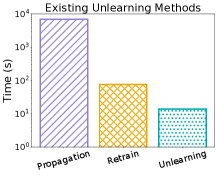
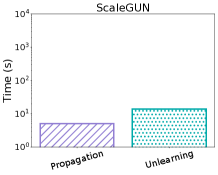
Figure 1: Time costs per $5K$-random-edge batch removal for existing unlearning methods v.s. ScaleGUN on ogbn-papers100M (2-hop SGC model).

This difference indicates that graph propagation, rather than training model parameters, is the primary bottleneck on large graphs.

To mitigate the costly graph propagation, extensive research efforts have been made in recent years to achieve scalable GNNs. These studies can be broadly categorized into three groups: (1) Sampling techniques (29; 11; 57; 15; 53). (2) Historical embedding methods (23; 10). (3) Decoupled models (46; 6; 44; 13). However, these approaches cannot be directly applied to certified graph unlearning, as they introduce approximation errors into the embeddings, and the effects of these errors on certified unlearning are not well understood. Consequently, whether these techniques can be integrated into certified graph unlearning to improve scalability remains an open and non-trivial problem.

In this work, we tackle this problem and take the first step to scale certified graph unlearning to billion-edge graphs. Specifically, we incorporate the approximate propagation technique from decoupled models into certified graph unlearning, and successfully derive the certified guarantees by detailed theoretical analysis of the effects of the approximation errors. Our main contributions are as follows.

• Theoretical analysis of certified guarantees. We develop a certified graph unlearning mechanism that employs the approximate embeddings with bounded error. As the first work to apply approximate propagation in certified unlearning, we reveal that the model error caused by approximation can also be “masked” by the perturbation. We derive the bounds of $\left\lVert\mathcal{L}(\mathbf{w}^{-},\mathcal{D}^{\prime})\right\rVert$ for all three graph unlearning scenarios by non-trivial analysis, innovatively linking the embeddings pre- and post-unlearning via our propagation framework. Compared to the existing graph unlearning methods that use exact embeddings, our approach introduces slightly more model error but significantly reduces the propagation costs by avoiding exact propagation for each removal.

• Lazy local propagation framework. To align with current unlearning methods and ensure applicability to typical propagation schemes, we extend the existing dynamic Personalized PageRank (PPR) algorithms (54; 55) to a lazy local propagation framework for Generalized PageRank scheme.

• Empirical studies. Extensive experiments on real-world datasets demonstrate the efficiency and efficacy of ScaleGUN. For instance, to achieve $(\epsilon,\delta)=(1,10^{-4})$ certified unlearning on ogbn-papers100M and remove $5K$-random-edge from the model, existing methods (17; 48) require over $6\times 10^{3}$ seconds (including propagation and unlearning cost in Figure 1). In contrast, ScaleGUN takes only $5$ seconds to update embeddings and an additional $14$ seconds to perform unlearning. We also empirically examine the impact of the approximation parameter $r_{\max}$, and observe that selecting a suitable $r_{\max}$ can achieve superior model accuracy and unlearning efficiency.

2 Preliminaries

Notation. We consider an undirected graph $\mathcal{G}=(\mathcal{V},\mathcal{E})$ with node set $\mathcal{V}$ of size $n$ and edge set $\mathcal{E}$ of size $m$. We denote the size of the training set as $n_{t}$. Each node is associated with an $F$-dimensional feature vector $\mathbf{x}$, and the feature matrix is denoted by $\mathbf{X}\in\mathbb{R}^{n\times F}$. $\mathbf{A}$ and $\mathbf{D}$ are the adjacency matrix and the diagonal degree matrix of $\mathcal{G}$ with self-loops, respectively. $\mathcal{N}(u)$ represents the neighbors of node $u$. Let $\mathcal{A}$ be a (randomized) learning algorithm that trains on graph-structured data $\mathcal{D}=(\mathbf{X},\mathbf{Y},\mathbf{A})\in\mathcal{X}$, where $\mathbf{Y}$ are the labels of the training nodes and $\mathcal{X}$ represents the space of possible datasets. $\mathcal{A}$ outputs a model $h\in\mathcal{H}$, where $\mathcal{H}$ is the hypothesis set, that is, $\mathcal{A}:\{\mathcal{D}\}\rightarrow\mathcal{H}$. Suppose that $\mathcal{D}^{\prime}$ is the new graph dataset resulting from a desired removal. An unlearning method $\mathcal{M}$ applied to $\mathcal{A}(\mathcal{D})$ will output a new model $h\in\mathcal{H}$ according to the unlearning request, that is $\mathcal{M}(\mathcal{A}(\mathcal{D}),\mathcal{D},\mathcal{D}^{\prime})\rightarrow\mathcal{H}$. We add a hat to a variable to denote the approximate version of it, e.g., $\mathbf{\hat{Z}}$ is the approximation of the embedding matrix $\mathbf{Z}$. For simplicity, we denote the data as $\hat{\mathcal{D}}$ to indicate that $\mathbf{\hat{Z}}$ takes the place of $\mathbf{Z}$ during the learning and unlearning process. We add a prime to a variable to denote the variable after the removal, e.g., $\mathcal{D}^{\prime}$ is the new dataset post-unlearning. In this paper, we interchangeably use certified removal and certified unlearning, certifiable and certified.

Certified removal. Guo et al. (27) define certified removal for unstructured data as follows. Given $\epsilon,\delta>0$, the original dataset $\mathcal{D}$, a removal request resulting in $\mathcal{D}^{\prime}$, a removal mechanism $\mathcal{M}$ guarantees $(\epsilon,\delta)$-certified removal for a learning algorithm $\mathcal{A}$ if $\forall\mathcal{T}\subseteq\mathcal{H},\mathcal{D}\subseteq\mathcal{X}$,

$$\begin{array}[]{r}\mathbb{P}(\mathcal{M}(\mathcal{A}(\mathcal{D}),\mathcal{D},\mathcal{D}^{\prime})\in\mathcal{T})\leq e^{\epsilon}\mathbb{P}(\mathcal{A}(\mathcal{D}^{\prime})\in\mathcal{T})+\delta,\text{ and }\\ \mathbb{P}(\mathcal{A}(\mathcal{D}^{\prime})\in\mathcal{T})\leq e^{\epsilon}\mathbb{P}(\mathcal{M}(\mathcal{A}(\mathcal{D}),\mathcal{D},\mathcal{D}^{\prime})\in\mathcal{T})+\delta.\end{array}$$

This definition states the likelihood ratio between the retrained model on $\mathcal{D}^{\prime}$ and the unlearned model via $\mathcal{M}$ is approximately equivalent in terms of their probability distributions. Guo et al. (27) also introduced a certified unlearning mechanism for linear models trained on unstructured data. Consider $\mathcal{A}$ trained on $\mathcal{D}=\{(\mathbf{x}_{1},y_{1}),\cdots,(\mathbf{x}_{n},y_{n})\}$ aiming to minimize the empirical risk $\mathcal{L}(\mathbf{w};\mathcal{D})=\sum_{i=1}^{n}l\left(\mathbf{w}^{\top}\mathbf{x}_{i},y_{i}\right)+\frac{\lambda n}{2}\|\mathbf{w}\|_{2}^{2}$, where $l$ is a convex loss function that is differentiable everywhere. Let $\mathbf{w}^{\star}=\mathcal{A}(\mathcal{D})$ be the unique optimum such that $\nabla\mathcal{L}(\mathbf{w}^{\star},\mathcal{D})=0$. Guo et al. propose the Newton udpate removal mechanism: $\mathbf{w}^{-}=\mathbf{w}^{\star}+\mathbf{H}_{\mathbf{w}^{\star}}^{-1}\Delta$, where $\Delta=\lambda\mathbf{w}^{\star}+\nabla l((\mathbf{w}^{\star})^{\top}\mathbf{x},y)$ when $(\mathbf{x},y)$ is removed, and $\mathbf{H}_{\mathbf{w}^{\star}}$ is the Hessian matrix of $\mathcal{L}(\cdot,\mathcal{D}^{\prime})$ at $\mathbf{w}^{\star}$. Furthermore, to mask the direction of the gradient residual $\nabla\mathcal{L}(\mathbf{w}^{-},\mathcal{D}^{\prime})$, they introduce a perturbation in the empirical risk: $\mathcal{L}_{\mathbf{b}}(\mathbf{w},\mathcal{D})=\mathcal{L}(\mathbf{w},\mathcal{D})+\mathbf{b}^{\top}\mathbf{w}$, where $\mathbf{b}\in\mathbb{R}^{F}$ is a random vector sampled from a specific distribution. Then, one can secure a certified guarantee by using the following theorem:

Theorem 2.1 (Theorem 3 in (27)).

Let $\mathcal{A}$ be the learning algorithm that returns the unique optimum of the loss $\mathcal{L}_{\mathbf{b}}(\mathbf{w};\mathcal{D})$. Suppose that a removal mechanism $\mathcal{M}$ returns $\mathbf{w}^{-}$ with $\left\|\nabla\mathcal{L}\left(\mathbf{w}^{-};\mathcal{D}^{\prime}\right)\right\|_{2}\leq\epsilon^{\prime}$ for some computable bound $\epsilon^{\prime}>0$. If $\mathbf{b}\sim\mathcal{N}\left(0,c\epsilon^{\prime}/\epsilon\right)^{d}$ with $c>0$, then $\mathcal{M}$ guarantees $(\epsilon,\delta)$-certified removal for $\mathcal{A}$ with $\delta=1.5\cdot e^{-c^{2}/2}$.

Certified graph unlearning. CGU (17) generalizes the certified removal mechanism to graph-structured data on SGC and the Generalized PageRank extensions. The empirical risk is modified to $\mathcal{L}(\mathbf{w};\mathcal{D})=\sum_{i=1}^{n_{t}}l\left(\mathbf{e}_{i}^{\top}\mathbf{Z}\mathbf{w},\mathbf{e}_{i}^{\top}\mathbf{Y}\right)+\frac{\lambda n_{t}}{2}\|\mathbf{w}\|_{2}^{2}$, where $\mathbf{e}_{i}^{\top}\mathbf{Z}=\mathbf{e}_{i}^{\top}(\mathbf{D}^{-1}\mathbf{A})^{k}\mathbf{X},\mathbf{e}_{i}^{\top}\mathbf{Y}$ is the embedding vector and the label of node $i$, respectively, and $n_{t}$ denotes the number of training nodes. Removing a node alters its neighbors’ embeddings, consequently affecting their loss values. Therefore, CGU generalizes the mechanism in (27) by revising $\Delta$ as $\nabla\mathcal{L}(\mathbf{w}^{\star},\mathcal{D})-\nabla\mathcal{L}(\mathbf{w}^{\star},\mathcal{D}^{\prime})$. If no graph structure is present, implying $\mathbf{Z}$ is independent of the graph structure, CGU aligns with that of (27). Based on the modifications, CGU derives the certified unlearning guarantee for three types of removal requests: node feature, edge, and node unlearning. Similarly, CEU (48) achieves certified unlearning for edge batch removal inspired by influence function (33).

Forward Push in graph propagation. Forward Push (4; 50) is a canonical technique designed to accelerate graph propagation computations for decoupled models (44; 13). The technique is a localized version of cumulative power iteration, performing one push operation for a single node at a time. Take Forward Push for $\mathbf{z}=\mathbf{P}^{\ell}\mathbf{x}$ and $\mathbf{P}=\mathbf{A}\mathbf{D}^{-1}$ as an example, where $\mathbf{x}$ is the graph signal vector and $\ell$ is the number of propagation steps. Forward Push maintains a reserve vector $\boldsymbol{q}^{(\ell)}$ and a residue vector $\boldsymbol{r}^{(\ell)}$ for each level $\ell$. For any node $u\in\mathcal{V}$, $\boldsymbol{q}^{(\ell)}(u)$ represents the current estimation of $(\mathbf{P}^{\ell}\mathbf{x})(u)$, and $\boldsymbol{r}^{(\ell)}(u)$ holds the residual mass to be distributed to subsequent levels. When $\boldsymbol{r}^{(\ell)}(u)$ exceeds a predefined threshold $r_{\max}$, it is added to $\boldsymbol{q}^{(\ell)}(u)$ and distributed to the residues of $u$’s neighbors in the next level, i.e., $\boldsymbol{r}^{(\ell+1)}(v)$ is increased by $\boldsymbol{r}^{(\ell)}(u)/d(u)$ for $v\in\mathcal{N}(u)$. After that, $\boldsymbol{r}^{(\ell)}(u)$ is set to $0$. Ignoring small residues that contribute little to the estimate, Forward Push  achieve a balance between estimation error and efficiency.

Dynamic PPR algorithms. Zhang et al. (54) proposed the first approximate PPR algorithm for dynamic graphs (56). Instant (55) extended this work to solve PPR-based propagation in evolving graphs, and DynamicPPE (28) adopted a similar idea to learn a target subset of node embeddings in dynamic networks. We focus on InstantGNN as the lazy local propagation framework in our ScaleGUN draws inspiration from it. Specifically, InstantGNN observed that the invariant property $\hat{\boldsymbol{\pi}}+\alpha\boldsymbol{r}=\alpha\mathbf{x}+(1-\alpha)\mathbf{P}\hat{\boldsymbol{\pi}}$ holds during the propagation process for the propagation scheme ${\boldsymbol{\pi}}=\sum_{\ell=0}^{\infty}\alpha(1-\alpha)^{\ell}\mathbf{P}^{\ell}\mathbf{x}$. Upon an edge arrival or removal, this invariant is disrupted due to the revised $\mathbf{P}$ or $\mathbf{x}$. InstantGNN updates the residue vector $\boldsymbol{r}$ for affected nodes to maintain the invariant, then applies Forward Push to meet the error requirement. Since only a few nodes are affected by one edge change, the updates are local and efficient.

3 Lazy Local Propagation

This section introduces our lazy local propagation framework that generates approximate embeddings with a bounded $L_{2}$-error. To effectively capture the propagation scheme prevalent in current GNN models and align with the existing graph unlearning methods, we adopt the Generalized PageRank (GPR) approach (35) as the propagation scheme, $\mathbf{Z}=\sum_{\ell=0}^{L}w_{\ell}\left(\mathbf{D}^{-\frac{1}{2}}\mathbf{A}\mathbf{D}^{-\frac{1}{2}}\right)^{\ell}\mathbf{X}$, where $w_{\ell}$ is the weight of the $\ell$-th order propagation matrix and $\sum_{\ell=0}^{L}\left\lvert w_{\ell}\right\rvert\leq 1$. Note that this propagation scheme differs from that of CGU (17), which uses an asymmetric normalized matrix $\mathbf{P}=\mathbf{D}^{-1}\mathbf{A}$ and fixes $w_{\ell}={1}/{L}$. We introduce the initial propagation method for a signal vector $\mathbf{x}$ and the corresponding update method. The approximate embedding matrix $\mathbf{\hat{Z}}$ can be obtained by parallel adopting the method for each signal vector and putting the results together. Details and pseudo-codes of our propagation framework are provided in Appendix D.

Remark.

The lazy local propagation framework draws inspiration from the dynamic PPR method of InstantGNN (55) and extends it to the GPR propagation scheme. To the best of our knowledge, our framework is the first to achieve efficient embeddings update for the layered propagation scheme in evolving graphs, making it readily applicable to various models, such as SGC, GBP (13), and GDC (24). Utilizing the GPR scheme also enhances the generalizability of ScaleGUN, allowing one to replace our propagation framework with dynamic PPR methods to achieve certified unlearning for PPR-based GNNs. Note that InstantGNN cannot be directly applied to certified unlearning because the impact of approximation on the certified unlearning guarantees has not been well studied. This paper’s main contribution is addressing this gap. We establish certified guarantees for GNNs that use approximate embeddings, as detailed in Section 4. The differences between our propagation framework and existing propagation methods are further detailed in Appendix D.1.

For the initial propagation, we adopt Forward Push with $\mathbf{P}=\mathbf{A}\mathbf{D}^{-1}$, drawing from the observation that $(\mathbf{D}^{-\frac{1}{2}}\mathbf{A}\mathbf{D}^{-\frac{1}{2}})^{\ell}=\mathbf{D}^{-\frac{1}{2}}(\mathbf{A}\mathbf{D}^{-1})^{\ell}\mathbf{D}^{\frac{1}{2}}$. Initially, we normalize $\mathbf{x}$ to ensure $\left\lVert\mathbf{D}^{\frac{1}{2}}\mathbf{x}\right\rVert_{1}\leq 1$, and set the residue vector $\boldsymbol{r}^{(0)}=\mathbf{D}^{\frac{1}{2}}\mathbf{x}$. Applying Forward Push, we derive $\mathbf{\hat{z}}=\sum_{\ell=0}^{L}{w_{\ell}}\mathbf{D}^{-\frac{1}{2}}\boldsymbol{q}^{(\ell)}$ as the approximation of $\mathbf{z}=\sum_{\ell=0}^{L}w_{\ell}\left(\mathbf{D}^{-\frac{1}{2}}\mathbf{A}\mathbf{D}^{-\frac{1}{2}}\right)^{\ell}\mathbf{x}$. Any non-zero $\boldsymbol{r}^{(\ell)}$ holds the weight mass not yet passed on to subsequent levels, leading to the approximation error between $\mathbf{\hat{z}}$ and $\mathbf{z}$. During the propagation process, it holds that

$$\mathbf{z}=\sum_{\ell=0}^{L}{w_{\ell}}\mathbf{D}^{-\frac{1}{2}}\left(\boldsymbol{q}^{(\ell)}+\sum_{t=0}^{\ell}(\mathbf{A}\mathbf{D}^{-1})^{\ell-t}\boldsymbol{r}^{(t)}\right).$$ (1)

By examining $\sum_{\ell=0}^{L}w_{\ell}\mathbf{D}^{-\frac{1}{2}}\sum_{t=0}^{\ell}(\mathbf{A}\mathbf{D}^{-1})^{\ell-t}\boldsymbol{r}^{(t)}$, we establish the error bound of $\mathbf{\hat{z}}$ as follows.

Lemma 3.1.

Given graph $\mathcal{G}$ with $n$ nodes and the threshold $r_{\max}$, the approximate embedding $\mathbf{\hat{z}}$ for signal vector $\mathbf{x}$ satisfies that $\left\lVert\mathbf{\hat{z}}-\mathbf{z}\right\rVert_{2}\leq\sqrt{n}Lr_{\max}$.

Inspired by the update method for the PPR-based propagation methods on dynamic graphs (55), we identify the invariant property for the GPR scheme as follows.

Lemma 3.2.

For each signal vector $\mathbf{x}$, the reserve vectors $\{\boldsymbol{q}^{(\ell)}\}$ and the residue vectors $\{\boldsymbol{r}^{(\ell)}\}$ satisfy the following invariant property for all $u\in\mathcal{V}$ during the propagation process:

$$\left\{\begin{aligned} &\boldsymbol{q}^{(\ell)}(u)+\boldsymbol{r}^{(\ell)}(u)=\mathbf{D}(u)^{\frac{1}{2}}\mathbf{x}(u),&\ell=0\\ &\boldsymbol{q}^{(\ell)}(u)+\boldsymbol{r}^{(\ell)}(u)=\sum_{t\in\mathcal{N}(u)}\frac{\boldsymbol{q}^{(\ell-1)}(t)}{d(t)},&0<\ell\leq L\\ \end{aligned}\right.$$ (2)

Upon a removal request, we adjust $\{\boldsymbol{r}^{(\ell)}\}$ locally for the affected nodes to maintain the invariant property. Consider an edge removal scenario, for example, where edge $(u,v)$ is targeted for removal. Only node $u$, node $v$, and their neighbors fail to meet Equation (2) due to the altered degrees of $u$ and $v$. Take the modification for node $u$ as an example. For level $0$, we update $\boldsymbol{r}^{(0)}(u)$ reflecting changes in $\mathbf{D}^{\frac{1}{2}}\mathbf{x}$. For subsequent levels, $\boldsymbol{r}^{(\ell)}(u)$ is updated to reflect that the right side of $u$’s equations exclude $\frac{\boldsymbol{q}^{(\ell-1)}(v)}{d(v)}$. For $u$’s neighbors, their residues are updated accordingly, since one term on the right, $\frac{\boldsymbol{q}^{(\ell-1)}(u)}{d(u)}$, shifts to $\frac{\boldsymbol{q}^{(\ell-1)}(u)}{d(u)-1}$. Post-adjustment, the invariant property is preserved across all nodes. Then we invoke Forward Push to secure the error bound and acquire the updated $\mathbf{\hat{z}}$. Removing a node can be treated as multiple edge removals by eliminating all edges connected to the node. Moreover, feature removal for node $u$ can be efficiently executed by setting $\boldsymbol{r}^{(0)}(u)$ as $-\boldsymbol{q}^{(0)}(u)$. The following theorem illustrates the average cost for each removal request.

Theorem 3.3 (Average Cost).

For a sequence of $m$ removal requests that remove all edges of the graph, the amortized cost per edge removal is $O\left(L^{2}d\right)$. For a sequence of $K$ random edge removals, the expected cost per edge removal is $O\left(L^{2}d\right)$.

Note that the propagation step $L$ and the average degree $d$ are both typically a small constant in practice. $L$ is commonly set to $2$ in GCN (32), SGC, GAT (42). Many real-world networks are reported to be scale-free, characterized by a small average degree (5). For instance, the citation network ogbn-arxiv and ogbn-papers100M exhibit average degrees of $6$ and $14$, respectively. Consequently, this setup generally allows for constant time complexity for each removal request.

4 Scalable and Certifiable Unlearning Mechanism

This section presents the certified graph unlearning mechanism of ScaleGUN based on the approximate embeddings. Following existing works, we first study linear models with a strongly convex loss function and focus on binary node classification problems. We define the empirical risk as $\mathcal{L}(\mathbf{w},\mathcal{D})=\sum_{i\in[n_{t}]}\left(l(\mathbf{e}_{i}^{\top}\mathbf{\hat{Z}}\mathbf{w},\mathbf{e}_{i}^{\top}\mathbf{Y})+\frac{\lambda}{2}\left\lVert\mathbf{w}\right\rVert^{2}\right),$ where $l$ is a convex loss that is differentiable everywhere, $\mathbf{e}_{i}^{\top}\mathbf{\hat{Z}}$ and $\mathbf{e}_{i}^{\top}\mathbf{Y}$ represents the approximate embedding vector and the label of node $i$, respectively. Without loss of generality, we assume that the training set contains the first $n_{t}$ nodes. Suppose that $\mathbf{w}^{*}$ is the unique optimum of the original graph and an unlearning request results in a new graph $\mathcal{D}^{\prime}$. Our unlearning approach produces a new model $\mathbf{w}^{-}$ as follows: $\mathbf{w}^{-}=\mathbf{w}^{\star}+\hat{\mathbf{H}}_{\mathbf{w}^{\star}}^{-1}\Delta,$ where $\Delta=\nabla\mathcal{L}(\mathbf{w}^{\star},\hat{\mathcal{D}})-\nabla\mathcal{L}(\mathbf{w}^{\star},\hat{\mathcal{D}}^{\prime})$ and $\hat{\mathbf{H}}_{\mathbf{w}^{\star}}$ is the Hessian matrix of $\mathcal{L}(\cdot,\hat{\mathcal{D}}^{\prime})$ at $\mathbf{w}^{\star}$. We also introduce a perturbation in the loss function following (27) to hide information: $\mathcal{L}_{\mathbf{b}}(\mathbf{w},\mathcal{D})=\mathcal{L}(\mathbf{w},\mathcal{D})+\mathbf{b}^{\top}\mathbf{w},$ where $\mathbf{b}\in\mathbb{R}^{F}$ is a noise vector sampled from a specific distribution.

Compared to the unlearning mechanism, $\mathbf{w}^{-}=\mathbf{w}^{\star}+\mathbf{H}_{\mathbf{w}^{\star}}^{-1}\left(\nabla\mathcal{L}(\mathbf{w}^{\star},\mathcal{D})-\nabla\mathcal{L}(\mathbf{w}^{\star},\mathcal{D}^{\prime})\right)$, proposed by (17), our primary distinction lies in the approximation of embeddings. This also poses the main theoretical challenges in proving certified guarantees. According to Theorem 2.1, an unlearning mechanism can ensure $(\epsilon,\delta)$-certified graph unlearning if $\lVert\nabla\mathcal{L}(\mathbf{w}^{-},\mathcal{D}^{\prime})\rVert$ is bounded. Bounding $\lVert\nabla\mathcal{L}(\mathbf{w}^{-},\mathcal{D}^{\prime})\rVert$ is the main challenge to develop a certified unlearning mechanism. One of the leading contributions of (27; 18) is to establish the bounds for their proposed mechanisms. In the following, we elaborate on the bounds of $\lVert\nabla\mathcal{L}(\mathbf{w}^{-},\mathcal{D}^{\prime})\rVert$ of ScaleGUN under three graph unlearning scenarios: node feature, edge, and node unlearning. Before that, we make the following assumptions.

Assumption 4.1.

For any dataset $\mathcal{D}\in\mathcal{X},i\in[n]$ and $\mathbf{w}\in\mathbb{R}^{F}$: (1) $\left\lVert\nabla l(\mathbf{e}_{i}^{\top}\mathbf{Z}\mathbf{w},\mathbf{e}_{i}^{\top}\mathbf{Y})\right\rVert\leq c$; (2) $l^{\prime}$ is $c_{1}$-bounded; (3) $l^{\prime}$ is $\gamma_{1}$-Lipschitz; (4) $l^{\prime\prime}$ is $\gamma_{2}$-Lipschitz; (5) $\left\lVert\mathbf{e}_{i}^{\top}\mathbf{X}\right\rVert\leq 1$.

Note that these assumptions are also needed for (17). Assumptions (1)(3)(5) can be avoided when working with the data-dependent bound in Theorem 4.5. We first focus on a single instance unlearning and extend to multiple unlearning requests in Section 4.3.

4.1 Node feature unlearning

We follow the definitions of all three graph unlearning scenarios in (17). In the node feature unlearning case, the feature and label of a node are removed, resulting in $\mathcal{D}^{\prime}=(\mathbf{X}^{\prime},\mathbf{Y}^{\prime},\mathbf{A})$, where $\mathbf{X}^{\prime}$ and $\mathbf{Y}^{\prime}$ is identical to $\mathbf{X}$ and $\mathbf{Y}$ except the row of the removed node is zero. Without loss of generality, we assume that the removed node is node $u$ in the training set. Our conclusion remains valid even when the removed node is not included in the training set.

Theorem 4.2 (Worst-case bound of node feature unlearning).

Suppose that Assumption 4.1 holds and the feature of node $u$ is to be unlearned. If $\forall j\in[F]$, $\left\lVert\hat{\mathbf{Z}}\mathbf{e}_{j}-\mathbf{Z}\mathbf{e}_{j}\right\rVert\leq\epsilon_{1}$, we have

$$\left\lVert\nabla\mathcal{L}(\mathbf{w}^{-},\mathcal{D}^{\prime})\right\rVert\leq\left(\frac{c\gamma_{1}}{\lambda}F+c_{1}\sqrt{F(n_{t}-1)}\right)\left(\epsilon_{1}+\frac{8{\gamma_{1}}F}{\lambda(n_{t}-1)}\cdot\sqrt{d(u)}\right).$$

The feature dimension $F$ affects the outcome as the analysis is conducted on one dimension of the embedding $\mathbf{Z}_{j}$ rather than on $\mathbf{e}_{i}^{\top}\mathbf{Z}$. In real-world datasets, $F$ is typically a small constant. Note that $\epsilon_{1}$ is exactly $\sqrt{n}Lr_{\max}$ according to Lemma 3.1. To ensure that the norm will not escalate with the training set size $n_{t}$, we typically set $\epsilon_{1}=O(\frac{1}{\sqrt{n_{t}}})$, which implies that $r_{\max}=O(1/\sqrt{n_{t}n})$. The bound can be viewed as comprising two components: the component resulting from approximation, $\left(\frac{c\gamma_{1}}{\lambda}F+c_{1}\sqrt{F(n_{t}-1)}\right)\epsilon_{1}$, and the component resulting from unlearning, $\left(\frac{c\gamma_{1}}{\lambda}F+c_{1}\sqrt{F(n_{t}-1)}\right)\frac{8{\gamma_{1}}F}{\lambda(n_{t}-1)}\cdot\sqrt{d(u)}$. In the second component, the norm increases if the unlearned node possesses a high degree, as removing a large-degree node’s feature impacts the embeddings of many other nodes. This component is not affected by $L$, the propagation step, due to the facts that $(\mathbf{D}^{-\frac{1}{2}}\mathbf{A}\mathbf{D}^{-\frac{1}{2}})^{\ell}=\mathbf{D}^{-\frac{1}{2}}(\mathbf{A}\mathbf{D}^{-1})^{\ell}\mathbf{D}^{\frac{1}{2}}$ and that $\mathbf{A}\mathbf{D}^{-1}$ is left stochastic.

Analytical challenges. It is observed that $\left\lVert\nabla\mathcal{L}(\mathbf{w}^{-},\mathcal{D}^{\prime})\right\rVert$ originates from the exact embeddings of $D^{\prime}$, whereas $\mathbf{w}^{-}$ is derived from approximate embeddings in ScaleGUN. Thus, the first challenge is to establish the connection between $\mathcal{D}^{\prime}$ and $\hat{\mathcal{D}}^{\prime}$ in $\left\lVert\nabla\mathcal{L}(\mathbf{w}^{-},\mathcal{D}^{\prime})\right\rVert$. To address this issue, we employ the Minkowski inequality to adjust the norm: $\left\lVert\nabla\mathcal{L}(\mathbf{w}^{-},\mathcal{D}^{\prime})\right\rVert\leq\left\lVert\nabla\mathcal{L}(\mathbf{w}^{-},\mathcal{D}^{\prime})-\nabla\mathcal{L}(\mathbf{w}^{-},\hat{\mathcal{D}}^{\prime})\right\rVert+\left\lVert\nabla\mathcal{L}(\mathbf{w}^{-},\hat{\mathcal{D}}^{\prime})\right\rVert.$ The first norm depicts the difference between the gradient of $\mathbf{w}^{-}$ on the exact and approximate embeddings, which is manageable through the approximation error. The second norm, $\left\lVert\nabla\mathcal{L}(\mathbf{w}^{-},\hat{\mathcal{D}}^{\prime})\right\rVert$, signifies the error of $\mathbf{w}^{-}$ as the minimizer of $\mathcal{L}(\cdot,\hat{\mathcal{D}}^{\prime})$, given as

$$\left\lVert\nabla\mathcal{L}(\mathbf{w}^{-},\hat{\mathcal{D}}^{\prime})\right\rVert=\left\lVert(\hat{\mathbf{H}}_{\mathbf{w}_{\eta}}-\hat{\mathbf{H}}_{\mathbf{w}^{\star}})\hat{\mathbf{H}}_{\mathbf{w}^{\star}}^{-1}\Delta\right\rVert,$$

where $\hat{\mathbf{H}}_{\mathbf{w}_{\eta}}$ is the Hessian of $\mathcal{L}(\cdot,\hat{\mathcal{D}}^{\prime})$ at $\mathbf{w}_{\eta}=\mathbf{w}^{\star}+\eta\hat{\mathbf{H}}_{\mathbf{w}^{\star}}^{-1}\Delta$ for some $\eta\in[0,1]$. This introduces the second challenge: bounding $\left\lVert\Delta\right\rVert$. Bounding $\left\lVert\Delta\right\rVert$ is intricate, especially for graph unlearning scenarios. Here, $\Delta$ represents the difference between the gradient of $\mathbf{w}^{*}$ on pre- and post-removal datasets, i.e., $\mathbf{\hat{Z}}$ and $\mathbf{\hat{Z}}^{\prime}$. Therefore, establishing the mathematical relationship between $\mathbf{Z}$ and $\mathbf{Z}^{\prime}$ is the crucial point. Although prior studies have explored the bound of $\left\lVert\mathbf{e}_{i}^{\top}(\mathbf{Z}-\mathbf{Z}^{\prime})\right\rVert$, their interest primarily lies in $\mathbf{P}=\mathbf{D}^{-1}\mathbf{A}$ (17) or $1$-hop feature propagation (48), which cannot be generalized to our GPR propagation scheme with $\mathbf{P}=\mathbf{D}^{-\frac{1}{2}}\mathbf{A}\mathbf{D}^{-\frac{1}{2}}$. We address this challenge innovatively by taking advantage of our lazy local propagation framework.

bounding $\left\lVert\Delta\right\rVert$ via the propagation framework. Assuming node $u$ is the $n_{t}$-th node in the training set, for the case of feature unlearning, we have

$$\Delta=\lambda\mathbf{w}^{\star}+\nabla l(\mathbf{\hat{Z}},\mathbf{w}^{\star},n_{t})+\sum_{i\in[n_{t}-1]}\left(\nabla l(\mathbf{\hat{Z}},\mathbf{w}^{\star},i)-\nabla l(\mathbf{\hat{Z}}^{\prime},\mathbf{w}^{\star},i)\right),$$

where $l(\mathbf{\hat{Z}},\mathbf{w}^{\star},i)$ is short for $l(\mathbf{e}_{i}^{\top}\mathbf{\hat{Z}}\mathbf{w}^{\star},\mathbf{e}_{i}^{\top}\mathbf{Y})$. Creatively, we bound $\left\lVert\mathbf{Z}\mathbf{e}_{j}-\mathbf{Z}^{\prime}\mathbf{e}_{j}\right\rVert$ for all $j\in[F]$ via the lazy local propagation framework. Let $\mathbf{z}=\mathbf{Z}\mathbf{e}_{j}$ and $\mathbf{z}^{\prime}=\mathbf{Z}^{\prime}\mathbf{e}_{j}$ for brevity. In our propagation framework, right after adjusting the residues upon a removal, $\{\boldsymbol{q}^{(\ell)}\}$ remains unchanged. Moreover, Equation (1) holds during the propagation process. Thus, we have

$$\mathbf{z}-\mathbf{z}^{\prime}=\sum_{t=0}^{\ell}{w_{\ell}}\sum_{t=0}^{\ell}\mathbf{D}^{-\frac{1}{2}}(\mathbf{A}\mathbf{D}^{-1})^{\ell-t}\left(\boldsymbol{r}^{(t)}-\boldsymbol{r}^{\prime(t)}\right).$$

To derive $\boldsymbol{r}^{(t)}-\boldsymbol{r}^{\prime(t)}$, notice that Equation (1) is applicable across all $r_{\max}$ configurations. Setting $r_{\max}=0$ to eliminate error results in $\boldsymbol{r}^{(t)}$ becoming a zero vector. Thus, for the feature unlearning scenario, $\boldsymbol{r}^{(0)}-\boldsymbol{r}^{\prime(0)}$ is precisely $-\boldsymbol{q}^{(0)}(u)\mathbf{e}_{u}$, as only node $u$’s residue is modified. For $t>0$, $\boldsymbol{r}^{(t)}-\boldsymbol{r}^{\prime(t)}$ are all zero vectors since these residues are not updated. This solves the second challenge. The bounds for edge and node unlearning scenarios can be similarly derived via the lazy local framework, significantly streamlining the proof process compared to direct analysis of $\mathbf{Z}\mathbf{e}_{j}-\mathbf{Z}^{\prime}\mathbf{e}_{j}$.

4.2 Edge unlearning and node unlearning

In the edge unlearning case, we remove an edge $(u,v)$, resulting in $\mathcal{D}^{\prime}=(\mathbf{X},\mathbf{Y},\mathbf{A}^{\prime})$, where $\mathbf{A}^{\prime}$ is identical to $\mathbf{A}$ except that the entries for $(u,v)$ and $(v,u)$ are set to zero. The node feature and labels remain unchanged. The conclusion remains valid regardless of whether $u,v$ are in the training set.

Theorem 4.3 (Worst-case bound of edge unlearning).

Suppose that Assumption 4.1 holds, and the edge $(u,v)$ is to be unlearned. If $\forall j\in[F]$, $\left\lVert\hat{\mathbf{Z}}\mathbf{e}_{j}-\mathbf{Z}\mathbf{e}_{j}\right\rVert\leq\epsilon_{1}$, we can bound $\left\lVert\nabla\mathcal{L}(\mathbf{w}^{-},\mathcal{D}^{\prime})\right\rVert$ by

$$\frac{4c\gamma_{1}F}{\lambda n_{t}}+\left(\frac{c\gamma_{1}}{\lambda}F+c_{1}\sqrt{Fn_{t}}\right)\left(\epsilon_{1}+\frac{2{\gamma_{1}}F}{\lambda n_{t}}(2\epsilon_{1}+\frac{4}{\sqrt{d(u)}}+\frac{4}{\sqrt{d(v)}})\right).$$

We observe that the worst-case bound diminishes when the two terminal nodes of the removed edge have a large degree. This reduction occurs because the impact of removing a single edge from a node with many edges is relatively minor.

In the node unlearning case, removing a node $u$ results in $\mathcal{D}^{\prime}=(\mathbf{X}^{\prime},\mathbf{Y}^{\prime},\mathbf{A}^{\prime})$, where the entries regarding the removed node in all three matrices are set to zero. The bound can be directly inferred from Theorem 4.3 since unlearning node $u$ equates to eliminating all edges connected to node $u$. This upper bound indicates that the norm is related to the degree of node $u$ and that of its neighbors.

Theorem 4.4 (Worst-case bound of node unlearning).

Suppose that Assumption 4.1 holds and node $u$ is removed. If $\forall j\in[F]$, $\left\lVert\hat{\mathbf{Z}}\mathbf{e}_{j}-\mathbf{Z}\mathbf{e}_{j}\right\rVert\leq\epsilon_{1}$, we can bound $\left\lVert\nabla\mathcal{L}(\mathbf{w}^{-},\mathcal{D}^{\prime})\right\rVert$ by

$$\frac{4c\gamma_{1}F}{\lambda(n_{t}-1)}+\left(\frac{c\gamma_{1}}{\lambda}F+c_{1}\sqrt{F(n_{t}-1)}\right)\left(\epsilon_{1}+\frac{2{\gamma_{1}}F}{\lambda(n_{t}-1)}(2\epsilon_{1}+4\sqrt{d(u)}+\sum_{w\in\mathcal{N}(u)}\frac{4}{\sqrt{d(w)}})\right).$$

4.3 Unlearning algorithm

In this subsection, we introduce the unlearning procedure of ScaleGUN. Due to space limits, more practical considerations are deferred to Appendix B.1, including feasible loss functions, batch unlearning, and the limitations of ScaleGUN.

Data-dependent bound. The worst-case bounds may be loose in practice. Following the existing certified unlearning studies (27; 17), we examined the data-dependent norm as follows. Similar to the worst-case bounds, the data-dependent bound can also be understood as two components: the first term $2c_{1}\left\lVert\mathbf{1}^{\top}\boldsymbol{R}\right\rVert$ incurred by the approximation error and the second term $\gamma_{2}\left\lVert\mathbf{\hat{Z}}^{\prime}\right\rVert\left\lVert\hat{\mathbf{H}}_{\mathbf{w}^{\star}}^{-1}\Delta\right\rVert\left\lVert\mathbf{\hat{Z}}^{\prime}\hat{\mathbf{H}}_{\mathbf{w}^{\star}}^{-1}\Delta\right\rVert$ incurred by unlearning. The second term is similar to that of the existing works, except that it is derived from the approximate embeddings.

Theorem 4.5 (Data-dependent bound).

Let $\boldsymbol{R}^{(t)}\in\mathbb{R}^{n\times F}$ denote the residue matrix at level $t$, where the $j$-th column $\boldsymbol{R}^{(t)}\mathbf{e}_{j}$ represents the residue at level $t$ for the $j$-th signal vector. Let $\boldsymbol{R}$ be defined as the sum $\sum_{t=0}^{L}\boldsymbol{R}^{(t)}$. We can establish the following data-dependent bound:

$$\left\lVert\nabla\mathcal{L}(\mathbf{w}^{-},\mathcal{D}^{\prime})\right\rVert\leq 2c_{1}\left\lVert\mathbf{1}^{\top}\boldsymbol{R}\right\rVert+\gamma_{2}\left\lVert\mathbf{\hat{Z}}^{\prime}\right\rVert\left\lVert\hat{\mathbf{H}}_{\mathbf{w}^{\star}}^{-1}\Delta\right\rVert\left\lVert\mathbf{\hat{Z}}^{\prime}\hat{\mathbf{H}}_{\mathbf{w}^{\star}}^{-1}\Delta\right\rVert.$$

Sequential unlearning algorithm. Multiple unlearning requests can be solved sequentially. The unlearning process is similar to the existing works (17; 48), except that we employ the lazy local propagation framework for the initial training and each removal. Specifically, we select the noise standard deviation $\alpha$ and privacy parameter $\epsilon,\delta$, and compute the “privacy budget”. Once the accumulated data-dependent norm exceeds the budget, we retrain the model and reset the accumulated norm. Notably, only the component attributable to unlearning, i.e., the second term in Theorem 4.5, needs to be accumulated. This is because the first term represents the error caused by the current approximation error and does not depend on the previous results. We provide the pseudo-code and illustrate more details in Appendix B.2.

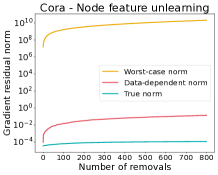
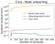
Figure 2: Comparison of the bounds of the gradient residual: Worst-case bound (Theorem 4.2, 4.3, 4.4 for node feature, edge, node unlearning, respectively), data-dependent bound (Theorem 4.5) and the true value on Cora dataset.

5 Experiments

In this section, we evaluate the performance of ScaleGUN on real-world datasets, including three small graph datasets: Cora (41), Citeseer (51), and Photo (37); as well as three large graph datasets: ogbn-arxiv, ogbn-products, and ogbn-papers100M (30). Consistent with prior certified unlearning research, we employ LBFGS as the optimizer for linear models. The public splittings are used for all datasets. Unless otherwise stated, we set $L=2,\epsilon=1,\delta=1e-4$ for all experiments, averaging results across $5$ trials with random seeds. Following (17), $w_{\ell}$ is set to 1 for $\ell=2$ and 0 for other values. Our benchmarks include CGU (17), CEU (12), and the standard retrain method. Note that $\delta$ can be configured to $\frac{1}{\rm\#edges}$ for edge unlearning and $\frac{1}{\rm\#nodes}$ for node/feature unlearning to meet higher privacy requirements (19; 40). The experimental results under this setting, other additional experiments and detailed configurations are available in Appendix C.

Metrics. We evaluate the performance of ScaleGUN in terms of efficiency, model utility, and unlearning efficacy. The efficiency is measured by the average total cost per removal and the average propagation cost per removal. The model utility is evaluated by the accuracy of node classification. We measure the unlearning efficacy in the task of forgetting adversarial data following (47).

Bounds on the gradient residual norm. Figure 2 validates the bounds on the gradient residual norm: the worst-case bounds, the data-dependent bounds, and the true value for all three unlearning scenarios on the Cora dataset. For simplicity, the standard deviation $\alpha$ is set to 0 for the noise $\bf{b}$. The results demonstrate that both the worst-case bounds and the data-dependent bounds validly upper bound the true value, and the worst-case bounds are looser than the data-dependent bounds.

Table 1: Test accuracy (%), total unlearning cost ($s$) and propagation cost ($s$) per batch edge removal for linear models (large graphs).

ogbn-arxiv					ogbn-products					ogbn-papers100M
$N$	Retrain	CGU	CEU	ScaleGUN	$N(\times 10^{3})$	Retrain	CGU	CEU	ScaleGUN	$N(\times 10^{3})$	Retrain	ScaleGUN
0	57.83	57.84	57.84	57.84	0	56.24	56.23	56.23	56.23	0	59.99	59.72
25	57.83	57.83	57.83	57.84	1	56.23	56.22	56.22	56.22	2	59.71	59.61
50	57.82	57.83	57.83	57.83	2	56.22	56.21	56.21	56.21	4	59.55	59.30
75	57.82	57.82	57.82	57.82	3	56.21	56.21	56.21	56.20	6	59.89	59.16
100	57.81	57.82	57.82	57.82	4	56.20	56.20	56.20	56.19	8	59.46	59.18
125	57.81	57.81	57.81	57.81	5	56.19	56.19	56.19	56.19	10	59.26	59.14
Total	2.66	2.28	2.08	0.91	Total	101.90	92.37	95.79	8.76	Total	6764.31	53.51
Prop	1.73	1.68	1.68	0.70	Prop	98.48	91.24	94.63	8.35	Prop	6703.44	6.14

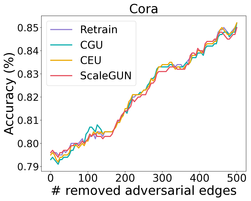
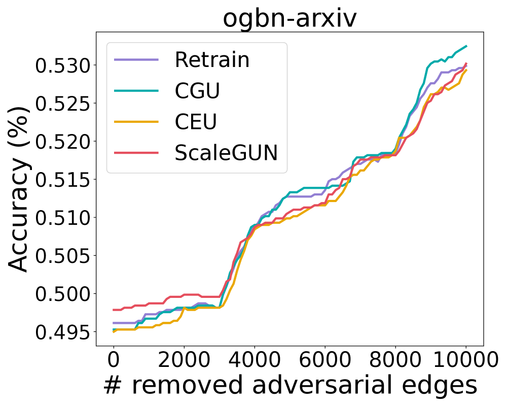
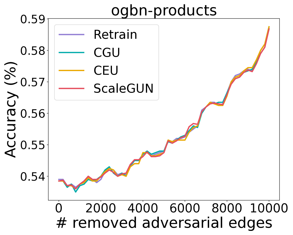
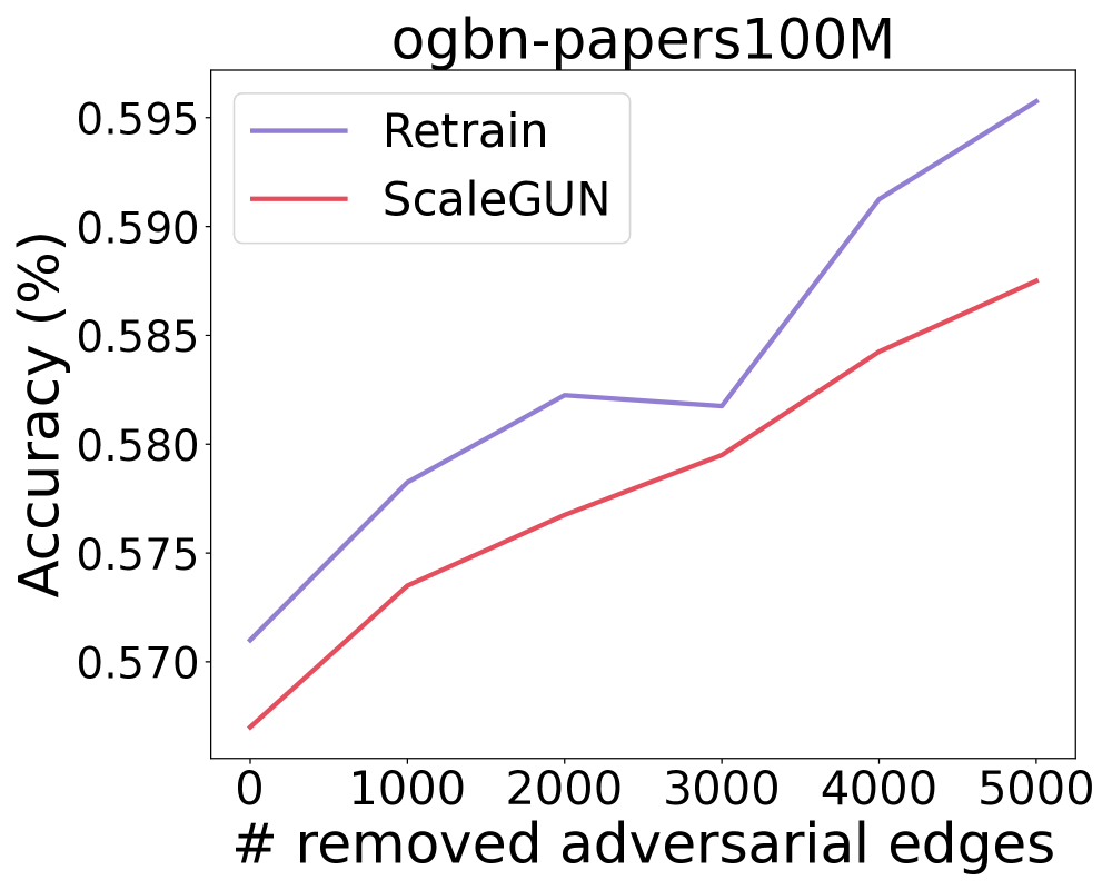
Figure 3: Comparison of unlearning efficacy for linear models: Model accuracy v.s. the number of removed adversarial edges.

Efficiency and model utility on linear models. Table 1 presents the test accuracy, average total unlearning cost, and average propagation cost for batch edge unlearning in linear models applied to large graph datasets. The results for small graphs are provided in Appendix C. For large datasets, randomly selecting edges to remove is insufficient to affect model accuracy significantly. We propose a novel approach to select a set of vulnerable edges for removal. Inspired by Theorem 4.3, we find that edges linked to nodes with small degrees are more likely to yield larger gradient residual norms, thus severely impacting performance. Consequently, we randomly choose a set of low-degree nodes from the test set and then select edges that connect these nodes to other low-degree nodes bearing identical labels. Table 1 details the accuracy after each batch unlearning and the average time cost per batch. The results highlight ScaleGUN’s impressive performance, with its advantages becoming more pronounced as the graph size increases. Notably, on the ogbn-papers100M dataset, ScaleGUN demonstrates a speed advantage of $1000\times$ over retraining in terms of propagation cost.

Table 2: Test accuracy (%), total unlearning cost ($s$) per batch edge removal for decoupled models.

ogbn-products			ogbn-papers100M
$N(\times 10^{3})$	Retrain	ScaleGUN	$N(\times 10^{3})$	Retrain	ScaleGUN
0	74.16	74.25	0	63.39	63.13
1	74.15	74.25	2	63.21	63.05
2	74.16	74.24	4	63.13	62.97
3	74.12	74.24	6	63.05	62.89
4	74.18	74.23	8	62.95	62.80
5	74.10	74.22	10	62.85	62.72
Total	174.23	14.19	Total	7958.83	10.49

Efficiency and model utility on deep models. When certified guarantees are relaxed, ScaleGUN can be applied to deep models to achieve better model utility. Table 2 presents ScaleGUN’s performance on decoupled models, where $2$-hop propagations followed by $2$-layer Multi-Layer Perceptrons (MLPs). We introduce perturbation $\mathbf{B}^{\top}\mathbf{W}$ to each learnable parameter $\mathbf{W}$, utilizing Adam as the optimizer. We exclude the propagation cost as its pattern is consistent with that in Table 1. This suggests that ScaleGUN can be employed in shallow networks to achieve higher accuracy when certified guarantees are not required. Additionally, ScaleGUN can be applied to spectral GNNs, a significant subset of GNNs rooted in spectral graph theory, known for their superior expressive power. The results using spectral GNNs as backbones are presented in Appendix C.

Unlearning efficacy. Acknowledging the absence of standardized methods for assessing data removal in graphs, existing unlearning studies employ attack methods to gauge unlearning efficacy. We adopt the approach proposed by (47). Specifically, we introduce adversarial edges into the graph, ensuring the terminal nodes bear different labels. These adversarial edges deceive the model into making incorrect predictions, diminishing its performance. The objective of unlearning is to delete these adversarial edges and recuperate the model’s performance. With the removal of more adversarial edges, the accuracy of unlearning methods is expected to rise, following the trend of retraining. Figure 3 illustrates how the model accuracy varies as the number of removed adversarial edges increases. The results affirm that CGU, CEU, and ScaleGUN exhibit effectiveness in unlearning.

Table 3: Initial test accuracy, total unlearning cost and propagation cost per edge removal by varying $r_{\max}$ on ogbn-arxiv with linear model.

$r_{\max}$	1e-5	1e-7	1e-9	5e-10	1e-10	1e-15
Acc (%)	55.23	57.84	57.84	57.84	57.84	57.84
Total (s)	3.30	3.60	3.31	1.81	0.92	0.93
Prop (s)	0.72	0.76	0.75	0.71	0.77	0.77
#Retrain	100	100	85.33	56.67	0	0

Effects of $r_{\max}$. ScaleGUN introduces the parameter $r_{\max}$ to manage the approximation error. To investigate the impact of $r_{\max}$, we conduct experiments on the ogbn-arxiv dataset, removing 100 random edges, one at a time. Table 3 displays the initial model accuracy before any removal, total unlearning cost, propagation cost per edge removal, and average number of retraining throughout the unlearning process. Decreasing $r_{\max}$ improves model accuracy and reduces the approximation error, leading to fewer retraining times and lower unlearning costs. Beyond a certain threshold, the model accuracy stabilizes, and the unlearning cost is minimized. Further reduction in $r_{\max}$ is unnecessary as it would increase the initial computational cost. Notably, the propagation cost remains stable, consistent with Theorem 3.3, which indicates that the average propagation cost is independent of $r_{\max}$. Table 3 suggests that selecting an appropriate $r_{\max}$ can achieve both high model utility and efficient unlearning.

6 Conclusion

This paper introduces ScaleGUN, the first certified graph unlearning mechanism that scales to billion-edge graphs. We introduce approximate propagation into certified unlearning and reveal the impact of approximation errors on the certified unlearning guarantees by non-trivial theoretical analysis. Certified guarantees are established for all three graph unlearning scenarios: node feature, edge, and node unlearning. Empirical studies of ScaleGUN on real-world datasets showcase its efficiency, model utility, and unlearning efficacy in graph unlearning.

Broader Impact

The proposed ScaleGUN is a scalable and certifiable graph unlearning method that aims to address the scalability challenge of the existing certified graph unlearning approaches. For applications in social networks and recommendation systems, applying ScaleGUN may improve the scalability of existing certified graph unlearning methods, thereby enhancing the privacy protection of users.

Appendix A Other Related Works

Machine unlearning, first introduced by Cao and Yang [2015], aims to eliminate the impact of selected training data from trained models to enhance privacy protection.

Exact unlearning. Exact unlearning seeks to generate a model that mirrors the performance of a model retrained from scratch. The straightforward method is to retrain the model upon a data removal request, which is often deemed impractical due to high computational and temporal costs. To bypass the burdensome retraining process, several innovative solutions have been proposed. Ginart et al. [2019] focused on $k$-means clustering unlearning, while Karasuyama and Takeuchi [2010] addressed the unlearning problem for support vector machines. Bourtoule et al. [2021] proposed the SISA (sharded, isolated, sliced, and aggregated) method, which partitions the training data into shards and trains on each shard separately. Upon a removal request, only the affected shards need to be retrained, thus enhancing the performance significantly. GraphEraser Chen et al. [2022] extended the SISA approach to graph-structured data. Projector and GraphEditor Cong and Mahdavi , Cong and Mahdavi [2023] address exact unlearning for linear GNNs with Ridge regression as their objective.

Approximate unlearning. Approximate unlearning, on the other hand, introduces probabilistic or heuristic methods to reduce unlearning costs further. Within this realm, certified unlearning, the primary subject of this study, stands as a subclass of approximate methods distinguished by its probabilistic assurances. Besides the certified unlearning works previously mentioned, Pan et al. [2023] extended the certified unlearning to graph scattering transform. GIF Wu et al. [2023a] developed graph influence function based on influence function for unstructured data Koh and Liang [2017]. Golatkar et al. [2020] proposed heuristic-based selective forgetting in deep networks. GNNDelete Cheng et al. [2023] introduced a novel layer-wise operator for optimizing deleted edge consistency and neighborhood influence in graph unlearning. Concurrently, Li et al. [2024] achieved effective and general graph unlearning through a mutual evolution design, and Wang et al. [2023] proposed the first general framework for addressing the inductive graph unlearning problem.

Differentially Privacy v.s. Certified unlearning. Differentially Privacy (DP) aims to ensure that an adversary cannot infer whether the model was trained on the original dataset or the dataset with any single data sample removed, based on the model’s output. Certified unlearning aims to remove the impact of the specific data sample(s) so that the model behaves as if the sample was never included. Thus, a DP model inherently provides certified unlearning for any single data sample. However, most DP models suffer from performance degradation even for loose privacy constraints Abadi et al. [2016], Chaudhuri et al. [2011]. Certified unlearning can balance model utility and computational cost, presenting an alternative to retraining and DP Chien et al. [2022b]. This also explains the growing interest in certified unlearning as privacy protection demands rise. Additionally, there are some nuances between DP and certified unlearning. For example, DP does not obscure the total dataset size and the number of deletions any given model instance has processed, but this should not be leaked in certified unlearning Ginart et al. [2019].

Appendix B Details of Certifiable Unlearning Mechanism

B.1 Practical Aspects

Least-squares and logistic regression on graphs. Similar to [Chien et al., 2022a], our unlearning mechanism can achieve certifiable unlearning with least-squares and binary logistic regression. ScaleGUN performs exact unlearning for least-squares since the Hessian of loss function is independent of $\mathbf{w}$. For binary logistic regression, we define the empirical risk as $l(\mathbf{e}_{i}^{\top}\mathbf{\hat{Z}}\mathbf{w},\mathbf{e}_{i}^{\top}\mathbf{Y}_{i})=-\log(\sigma(\mathbf{e}_{i}^{\top}\mathbf{Y}_{i}\mathbf{e}_{i}^{\top}\mathbf{\hat{Z}}\mathbf{w}))$, where $\sigma$ denotes the sigmoid function. As shown in Guo et al. [2019], Chien et al. [2022a], Assumption 4.1 holds with $c=1,\gamma_{1}=\gamma_{2}=1/4,c_{1}=1$ for logistic regression. Following Chien et al. [2022a], ScaleGUN can adapt the “one-versus-all other classes” strategy for multiclass logistic regression.

Batch unlearning. In the batch unlearning scenario, multiple instances may be removed at a time. In the worst-case bounds of the gradient residual norm, the component attributable to approximation error remains unchanged across three kinds of unlearning requests and for any number of unlearning instances. This stability is due to our lazy local propagation framework, which ensures the approximation error $\epsilon_{1}$ does not vary with the number of removed instances. Regarding the component related to unlearning, which is mainly determined by $\left\lVert\mathbf{Z}\mathbf{e}_{j}-\mathbf{Z}^{\prime}\mathbf{e}_{j}\right\rVert$, we can establish the corresponding bounds by aggregating the bounds for each unlearning instance, utilizing the Minkowski inequality. The data-dependent bound remains unchanged and can be computed directly.

Limitations of existing certified unlearning mechanisms. The existing certified unlearning studies, including ScaleGUN, are limited to linear models with a strongly convex loss function. Achieving certified graph unlearning in nonlinear models is a significant yet challenging objective. Existing approximate unlearning methods on deep models are heuristics without theoretical guarantees Golatkar et al. [2020], McAuley et al. [2015]. On the one hand, the theoretical foundation of existing certified unlearning mechanisms is the Newton update. However, the thorough examination of the Newton update in deep networks remains an unresolved issue Xu et al. [2018]. Koh and Liang [2017] demonstrates that the Newton update performs well in non-convex shallow CNN networks. However, performance may decline in deeper architectures as the convexity of the loss function is significantly compromised Wu et al. [2023a]. On the other hand, note that a certified unlearning model is approximately equivalent to retraining in terms of their probability distributions. This indicates that the unlearning model must be able to approximate the new optimal point of empirical risk within a certain margin of error after data removal. However, existing studies Wang and Pilanci [2023] have proven that even approximating the optimal value of a 2-layer ReLU neural network is NP-hard in the worst cases. Therefore, the path to certified unlearning in nonlinear models remains elusive, even for unstructured data. While ScaleGUN cannot achieve certified unlearning for deep models, our empirical results demonstrate that ScaleGUN can achieve competitive model utility using deep models as backbones when certified guarantees are not required, as shown in Table 2 and Table 14. In summary, ScaleGUN can perform certified unlearning for linear GNNs and serves as an effective heuristic unlearning method for deep models.

Input: Graph data $\mathcal{D}=(\mathbf{X},\mathbf{Y},\mathbf{A})$, sequence of removal requests $R=\{R_{1},\cdots,R_{k}\}$, loss function $l$, parameters $L,\{w_{\ell}\},r_{\max},\alpha,\gamma_{2},\epsilon,\delta$

1 Compute the embedding matrix $\mathbf{\hat{Z}}$ by Algorithm 2 with initialized $\{\boldsymbol{q}^{(\ell)}\}$ and $\{\boldsymbol{r}^{(\ell)}\}$ ;

2 $\mathbf{w}\leftarrow$ the model trained on the training set of $\hat{\mathcal{D}}$ with the approximate embeddings $\mathbf{\hat{Z}}$;

3 Accumulated unlearning error $\beta\leftarrow 0$;

4 for $R_{i}\in R$ do

5       $\mathbf{\hat{Z}}^{\prime},\boldsymbol{R}\leftarrow$ the embedding matrix updated by the lazy local propagation framework and the corresponding residue matrix according to the removal request $R_{i}$;

6       $\hat{\mathcal{D}}^{\prime}\leftarrow$ the updated dataset according to $R_{i}$;

7       $\Delta\leftarrow\nabla\mathcal{L}(\mathbf{w},\hat{\mathcal{D}})-\mathcal{L}(\mathbf{w},\hat{\mathcal{D}}^{\prime})$;

8       $\hat{\mathbf{H}}_{\mathbf{w}}\leftarrow\nabla^{2}\mathcal{L}(\mathbf{w},\hat{\mathcal{D}}^{\prime})$;

9       $\beta\leftarrow\beta+\gamma_{2}\left\lVert\mathbf{\hat{Z}}^{\prime}\right\rVert\left\lVert\hat{\mathbf{H}}_{\mathbf{w}^{\star}}^{-1}\Delta\right\rVert\left\lVert\mathbf{\hat{Z}}^{\prime}\hat{\mathbf{H}}_{\mathbf{w}^{\star}}^{-1}\Delta\right\rVert$;

10       if $\beta+2c_{1}\left\lVert\mathbf{1}^{\top}\boldsymbol{R}\right\rVert>\alpha\epsilon/\sqrt{2\log(1.5/\delta)}$ then

11             $\mathbf{w}\leftarrow$ the model retrained on the training set of $\hat{\mathcal{D}}^{\prime}$;

12             $\beta\leftarrow 0$;

13            

14      else

15            $\mathbf{w}=\mathbf{w}+\hat{\mathbf{H}}_{\mathbf{w}}^{-1}\Delta$;

16      

Algorithm 1 ScaleGUN

Potential improvements and future directions. As suggested in Guo et al. [2019], Chien et al. [2022a], pretraining a nonlinear feature extractor on public datasets can significantly improve overall model performance. If no public datasets are available, a feature extractor with differential privacy (DP) guarantees can be designed. DP-based methods provide privacy guarantees for nonlinear models, indicating the potential to leverage DP concepts to facilitate certified unlearning in deep models. We also observe that ScaleGUN is capable of data removal from deep models to a certain extent (see Figure 6 in Appendix C), even without theoretical guarantees. This observation suggests the possibility of formulating more flexible certification criteria to assess the efficacy of current heuristic approaches.

B.2 Details of sequential unlearning algorithm

According to the privacy requirement and Theorem 2.1, we select the noise standard deviation $\alpha$, privacy parameters $\epsilon,\delta$ and compute the “privacy budget” $\alpha\epsilon/\sqrt{2\log(1.5/\delta)}$. Initially, compute the approximate embeddings by the lazy local propagation framework and train the model from scratch. For each unlearning request, update the embeddings and then employ our unlearning mechanism. Specifically, compute the first component of the data-dependent bound, i.e., $2c_{1}\left\lVert\mathbf{1}^{\top}\boldsymbol{R}\right\rVert$ in Theorem 4.5 and accumulate the second component $\gamma_{2}\left\lVert\mathbf{\hat{Z}}^{\prime}\right\rVert\left\lVert\hat{\mathbf{H}}_{\mathbf{w}^{\star}}^{-1}\Delta\right\rVert\left\lVert\mathbf{\hat{Z}}^{\prime}\hat{\mathbf{H}}_{\mathbf{w}^{\star}}^{-1}\Delta\right\rVert$ for each unlearning request. Once the budget is exhausted, retrain the model from scratch. Note that we do not need to re-propagate even when retraining the model. Algorithm 1 provides the pseudo-code of ScaleGUN, where the removal request $R_{i}$ can be one instance or a batch of instances.

Table 4: Statistics of datasets.

Dataset	$n$	$m$	$|C|$	$F$	train/val/test
Cora	2708	5278	7	1433	1208/500/1000
Citeseer	3327	4552	6	3703	1827/500/1000
Photo	7650	119081	8	745	6150/500/1000
ogbn-arxiv	169,343	1,166,243	40	128	90941/29799/48603
ogbn-products	2,449,029	61,859,140	47	128	196615/39323/2213091
ogbn-papers100M	111,059,956	1,615,685,872	172	128	1,207,179/125,265/125,265

Table 5: Parameters used in the linear model experiments.

Dataset	$r_{\max}$	$\lambda$	$\alpha$
Cora	1e-7	1e-2	0.1
Citeseer	1e-8	1e-2	0.1
Photo	1e-8	1e-4	3.0
ogbn-arxiv	1e-8	1e-4	0.1
ogbn-products	1e-8	1e-4	0.1
ogbn-papers100M	1e-9	1e-8	15.0

Table 6: Parameters used in the deep model experiments.

Dataset	$\lambda$	$\alpha$	learning rate	hidden size	batch size
ogbn-arxiv	5e-4	0.1	1e-3	1024	1024
ogbn-products	1e-4	0.01	1e-4	1024	512
ogbn-papers100M	1e-8	5.0	1e-4	256	8192

Table 7: Test accuracy (%), total unlearning cost (s) and propagation cost (s) per node feature/feature removal for linear models on Cora and ogbn-arxiv.

Feature Unlearning								Node Unlearning
Cora				ogbn-arxiv				Cora				ogbn-arxiv
$N$	Retrain	CGU	ScaleGUN	$N$	Retrain	CGU	ScaleGUN	$N$	Retrain	CGU	ScaleGUN	$N$	Retrain	CGU	ScaleGUN
$0$	$84.9$	$84.9$	$84.9$	$0$	$57.84$	$57.84$	$57.84$	$0$	$84.9$	$84.9$	$84.9$	$0$	$57.84$	$57.84$	$57.84$
$200$	$84.17$	$83.4$	$83.4$	$25$	$57.83$	$57.84$	$57.84$	$200$	$83.5$	$82.97$	$82.97$	$25$	$57.83$	$57.83$	$57.84$
$400$	$84.4$	$82.43$	$82.43$	$50$	$57.83$	$57.83$	$57.83$	$400$	$82.43$	$81.53$	$81.53$	$50$	$57.83$	$57.83$	$57.83$
$600$	$83.03$	$81.73$	$81.73$	$75$	$57.84$	$57.84$	$57.84$	$600$	$81.87$	$80.7$	$80.7$	$75$	$57.84$	$57.84$	$57.84$
$800$	$81.9$	$77.83$	$77.83$	$100$	$57.83$	$57.85$	$57.84$	$800$	$80.1$	$76.7$	$76.7$	$100$	$57.83$	$57.84$	$57.84$
$T_{1}$	$0.44$	$0.20$	$0.10$	$T_{1}$	$2.59$	$2.33$	$1.49$	$T_{1}$	$0.44$	$0.20$	$0.11$	$T_{1}$	$2.66$	$2.04$	$1.38$
$T_{2}$	$0.11$	$0.10$	$0.01$	$T_{2}$	$1.55$	$1.56$	$0.77$	$T_{2}$	$0.10$	$0.10$	$0.01$	$T_{2}$	$1.66$	$1.43$	$0.81$

Table 8: Test accuracy (%), total unlearning cost (s), and propagation cost (s) per one-edge removal for linear models (small graphs).

Cora					Citeseer					Photo
$N(\times 500)$	Retrain	CGU	CEU	ScaleGUN	$N(\times 500)$	Retrain	CGU	CEU	ScaleGUN	$N(\times 500)$	Retrain	CGU	CEU	ScaleGUN
0	85.30	84.10	84.10	84.10	0	79.30	78.80	78.80	78.80	0	91.67	89.93	89.93	89.93
1	85.20	83.30	83.30	83.30	1	78.60	78.37	78.37	78.37	1	91.60	89.90	89.90	89.90
2	84.10	82.30	82.30	82.30	2	78.30	78.00	78.00	78.00	2	91.60	89.90	89.90	89.90
3	83.00	81.80	81.80	81.80	3	77.93	77.43	77.43	77.43	3	91.57	89.67	89.67	89.67
4	82.40	81.40	81.40	81.40	4	77.60	77.10	77.10	77.10	4	91.63	89.67	89.67	89.67
Total	0.74	0.28	0.32	0.12	Total	0.99	0.81	0.76	0.55	Total	3.08	0.35	0.40	0.07
Prop	0.15	0.15	0.17	0.01	Prop	0.34	0.29	0.27	0.03	Prop	0.31	0.26	0.29	0.01

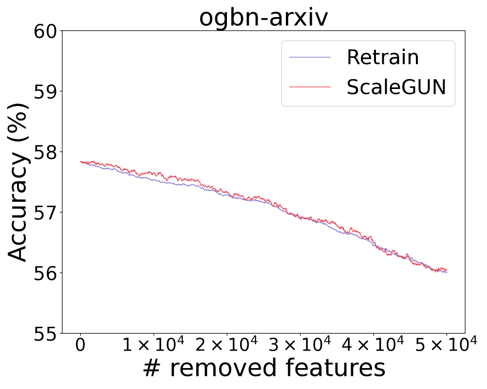
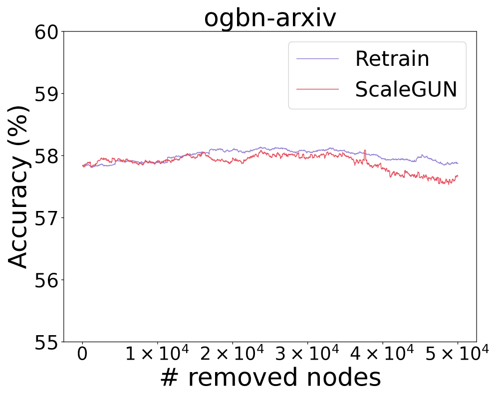
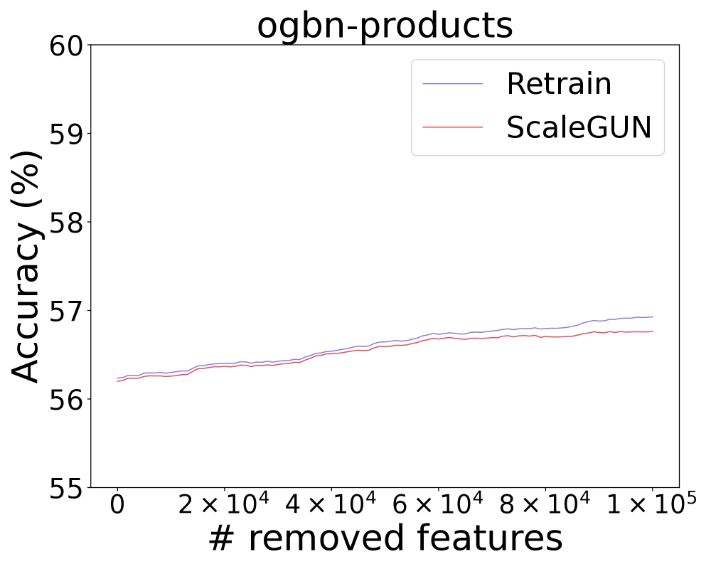
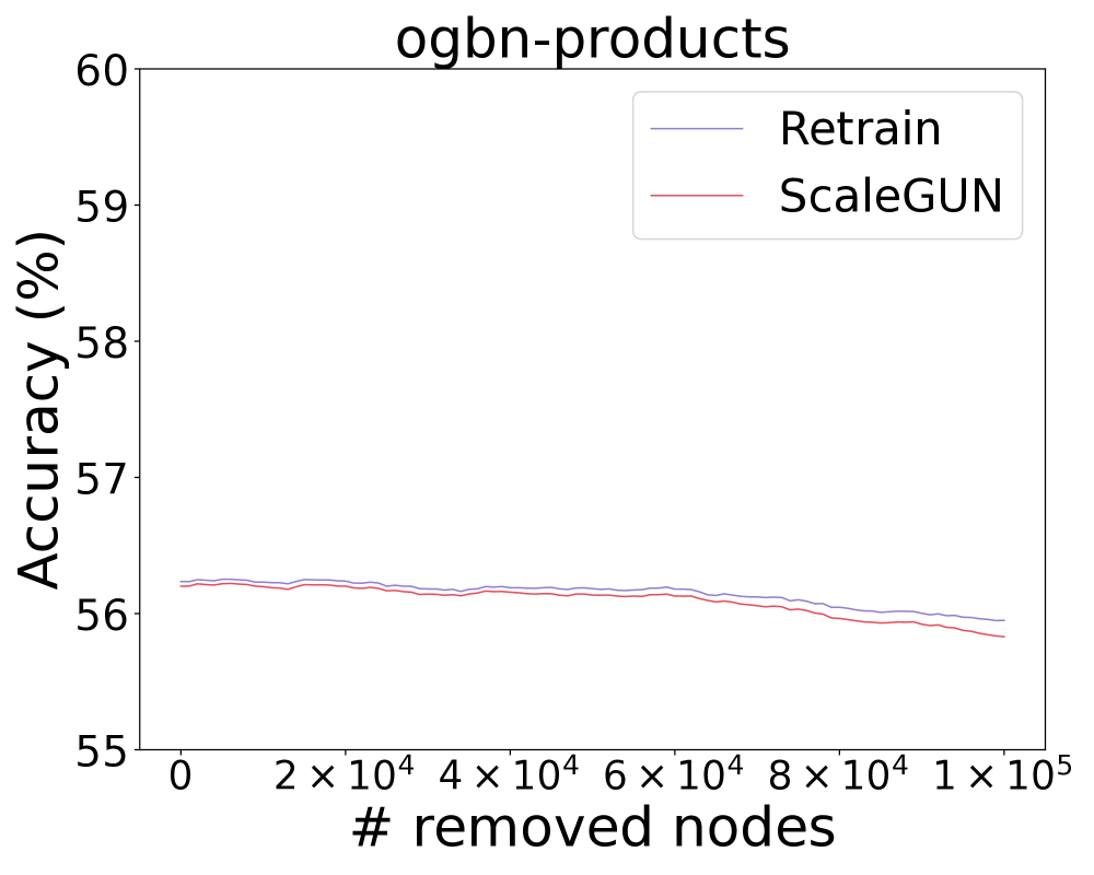
Figure 4: Unlearning more than 50% of training nodes/features: Test accuracy on ogbn-arxiv and ogbn-products.

Appendix C Details of Experiments and Additional Experiments

C.1 Experiments settings.

We use cumulative power iteration to compute exact embeddings for the retrain method, CGU, and CEU. Each dimension of the embedding matrix is computed in parallel with a total of 40 threads. We adopt the “one-versus-all” strategy to perform multi-class node classification following Chien et al. [2022a]. We conduct all experiments on a machine with an Intel(R) Xeon(R) Silver 4114 CPU @ 2.20GHz CPU, 1007GB memory, and Quadro RTX 8000 GPU in Linux OS. The statistics of the datasets are summarized in Table 4. Table 5 and Table 6 summarize the parameters used in the linear and deep experiments, respectively. The parameters are consistently utilized across all methods. Note that CGU Chien et al. [2022a] adopted $\mathbf{P}=\mathbf{D}^{-1}\mathbf{A}$ for analytical simplicity. In the experiments of this paper, we use $\mathbf{P}=\mathbf{D}^{-\frac{1}{2}}\mathbf{A}\mathbf{D}^{-\frac{1}{2}}$ across all the methods for fair comparison.

Adversarial edges selection. In Figure 3, we show the model accuracy as the number of removed adversarial edges increases. We add $500$ adversarial edges to Cora, with $5$ random edges being removed in each removal request. For ogbn-arxiv, ogbn-products, and ogbn-papers100M, we add $10^{4}$ adversarial edges, with batch-unlearning size as $100$, $200$, and $2000$, respectively. The details of selecting adversarial edges are as follows. For the Cora dataset, we randomly select edges connecting two distinct labeled terminal nodes and report the accuracy on the whole test set. For large datasets, randomly selecting adversarial edges proves insufficient to impact model accuracy. Hence, we initially identify a small set of nodes from the test set, then add adversarial edges by linking these nodes to other nodes with different labels. Specifically, we first randomly select 2000 nodes from the original test set to create a new test set $\mathcal{V}_{t}$. We then repeat the following procedure until we collect enough edges: randomly select a node $u$ from $\mathcal{V}_{t}$, randomly select a node $v$ from the entire node set $\mathcal{V}$, and if $u$ and $v$ have different labels, we add the adversarial edge $(u,v)$ to the original graph.

Vulnerable edges selection. In Table 1, we show the unlearning results in large graph datasets. For these datasets, we selected vulnerable edges connected to low-degree nodes in order to observe changes in test accuracy after unlearning. The details of selecting vulnerable edges are as follows. We first determine all nodes with a degree below a specified threshold in the test set. Specifically, the threshold is set to 10 for the ogbn-arxiv and ogbn-products datasets, and 6 for the ogbn-papers100M dataset. We then shuffle the set of these low-degree nodes and iterate over each node $v$: For each node $v$, if any of its neighbors share the same label as $v$, the corresponding edge is included in the unlearned edge set. The iteration ends until we collect enough edges.

C.2 More experiments on node feature, edge and node unlearning.

Node feature and node unlearning experiments. We conduct experiments on node feature and node unlearning for linear models and choose Cora, ogbn-arixv, and ogbn-papers100M as the representative datasets. Table 7 shows the model accuracy, average total cost, and average propagation cost per removal on Cora and ogbn-arxiv. For Cora, we remove the feature of one node at a time for node feature unlearning tasks. While for ogbn-arxiv, we remove the feature of 25 nodes. The node unlearning task is set in the same way. Table 9 shows the results on ogbn-papers100M, where 2000 edges are removed at a time. The results demonstrate that ScaleGUN achieves competitive accuracy compared to CGU and the retrained model while significantly reducing the total unlearning and propagation costs under the node feature and node unlearning scenario.

Table 9: Test accuracy (%), total unlearning cost (s) and propagation cost (s) per node feature/node removal for linear models on ogbn-papers100M.

Feature Unlearning			Node Unlearning
$N(\times 10^{3})$	Retrain	ScaleGUN	$N(\times 10^{3})$	Retrain	ScaleGUN
0	59.99	59.95	0	59.99	59.95
2	59.99	59.66	2	59.99	59.70
4	59.99	59.66	4	59.99	59.76
6	59.99	59.66	6	59.99	59.85
8	59.99	59.66	8	59.99	59.83
10	59.99	59.45	10	60.00	59.49
Total	5400.45	42.68	Total	5201.88	54.85
Prop	5352.84	5.90	Prop	5139.09	15.49

Edge unlearning results on small graphs. Table 8 presents test accuracy, average total unlearning cost, and average propagation cost for edge unlearning in linear models applied to small graph datasets. For each dataset, 2000 edges are removed, with one edge removed at a time. The table reports the initial and intermediate accuracy after every 500-edge removal. ScaleGUN is observed to maintain competitive accuracy when compared to CGU and CEU while notably reducing both the total and propagation costs. It is important to note that the difference in unlearning cost (Total$-$Prop) among the three methods is relatively minor. However, CGU and CEU incur the same propagation cost as retraining, which is $10\times\sim 30\times$ higher than that of ScaleGUN.

Model utility when removing more than 50% training nodes. To validate the model utility when the unlearning ratio reaches 50%, we remove $5\times 10^{4}$ and $10^{5}$ training nodes/features from ogbn-arxiv and ogbn-products in Figure 4. The batch-unlearning sizes are set to 25 and $10^{3}$ nodes/features, respectively. The results show that ScaleGUN closely matches the retrained model’s utility even when half of the training nodes/features are removed.

C.3 Parameter Studies.

Trade-off between privacy, model utility, and unlearning efficiency. According to Theorem 2.1 and our sequential unlearning algorithm, there is a trade-off amongst privacy, model utility, and unlearning efficiency. Specifically, $\epsilon$ and $\delta$ controls the privacy requirement. To achieve $(\epsilon,\delta)$-certified unlearning, we can adjust the standard deviation $\alpha$ of the noise $\mathbf{b}$. An overly large $\alpha$ introduces too much noise and may degrade the model utility. However, a smaller $\alpha$ may lead to frequent retraining and increase the unlearning cost due to the privacy budget constraint. We empirically analyze the trade-off between privacy and model utility following Chien et al. [2022a]. We remove 800 nodes from Cora, one at a time.

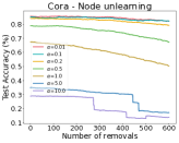
Figure 5: Varying $\alpha$ ($\alpha\epsilon=0.1$ fixed): Test accuracy v.s. the number of removed nodes on Cora.

To control the frequency of retraining, we fix $\alpha\epsilon=0.1$ and vary the standard derivation $\alpha$ of the noise $\bf{b}$. The results are shown in Figure 5. Here, we set $\delta=1/{\rm\#nodes}$ and $r_{\max}=1e-10$. We observe that the model accuracy decreases as $\alpha$ increases (i.e., $\epsilon$ decreases), which agrees with our intuition.

Varying batch-unlearning size. To validate the model efficiency and model utility under varying batch-unlearning sizes, we vary the batch-unlearning size in {$1\times 10^{3},3\times 10^{3},5\times 10^{3},10\times 10^{3}$} for ogbn-products and {$2\times 10^{3},10\times 10^{3},50\times 10^{3}$} for ogbn-papers100M in Table 10. The average total cost and propagation cost for five batches and the accuracy after unlearning five batches are reported. For comparison, the corresponding retraining results are provided, where $1\times 10^{3}$ and $2\times 10^{3}$ nodes are removed per batch for ogbn-products and ogbn-papers100M, respectively. ScaleGUN maintains superior efficiency over retraining, even when the batch-unlearning size becomes 4%-5% of the training set in large graphs (e.g., $50\times 10^{3}$ nodes in a batch out of $1.2\times 10^{6}$ total training nodes of ogbn-papers100M). The test accuracy demonstrates that ScaleGUN preserves model utility under varying batch-unlearning sizes.

Results on $\delta=\frac{1}{\rm\#edges}/\frac{1}{\rm\#nodes}$. Table 11 presents the batch edge unlearning results on large graphs with $\delta=\frac{1}{\rm\#edges}$. Modifying $\delta$ reduces the privacy budget slightly and potentially incurs more frequent retraining. Thus, we adjust $r_{\max}$ for each dataset to mitigate retraining requirements. Specifically, we set $r_{\rm max}=1e-10$ across all three datasets for simplicity. Despite these adjustments, Table 11 shows the superior performance of ScaleGUN. The node feature/node unlearning results exhibit similar trends and are omitted for brevity.

C.4 Additional Validation of Unlearning Efficacy.

Unlearning efficacy on deep models. We also evaluate the unlearning efficacy for deep models. Figure 6 shows how the model accuracy varies as the number of removed adversarial edges increases. The adversarial edges are the same as those used for linear models. The results demonstrate that ScaleGUN can effectively unlearn the adversarial edges even in shallow non-linear networks.

Table 10: Varying batch-unlearning size: Test accuracy (%), average total cost ($s$), and average propagation cost ($s$) per batch node removal.

Metric	ogbn-products					ogbn-papers100M
	ScaleGUN				Retrain	ScaleGUN			Retrain
	$1\times 10^{3}$	$3\times 10^{3}$	$5\times 10^{3}$	$10\times 10^{3}$	$1\times 10^{3}$	$2\times 10^{3}$	$10\times 10^{3}$	$50\times 10^{3}$	$2\times 10^{3}$
Acc	56.25	56.25	56.07	56.14	56.24	59.49	59.71	58.76	59.45
Total	24.00	39.07	45.58	56.14	92.44	54.85	352.35	657.99	5201.88
Prop	21.97	37.25	43.91	54.72	91.54	15.49	313.11	621.62	5139.09

Table 11: Test accuracy (%), total unlearning cost (s) and propagation cost (s) per batch edge removal for linear models (large graphs, $\delta=\frac{1}{\rm\#edges}$).

ogbn-arxiv					ogbn-products					ogbn-papers100M
$N$	Retrain	CGU	CEU	ScaleGUN	$N(\times 10^{3})$	Retrain	CGU	CEU	ScaleGUN	$N(\times 10^{3})$	Retrain	ScaleGUN
0	57.83	57.84	57.84	57.84	0	56.24	56.17	56.17	56.04	0	59.99	59.82
25	57.83	57.84	57.84	57.84	1	56.23	56.16	56.16	56.03	2	59.71	59.71
50	57.82	57.83	57.83	57.83	2	56.22	56.15	56.15	56.02	4	59.55	59.90
75	57.82	57.82	57.82	57.82	3	56.21	56.15	56.15	56.15	6	59.89	59.32
100	57.81	57.81	57.81	57.81	4	56.20	56.14	56.14	56.24	8	59.46	59.59
125	57.81	57.81	57.81	57.81	5	56.19	56.13	56.13	56.17	10	59.26	59.15
Total	2.66	3.36	3.42	1.08	Total	101.90	87.79	88.90	11.69	Total	6764.31	54.79
Prop	1.73	2.78	2.91	0.85	Prop	98.48	86.81	87.95	10.81	Prop	6703.44	9.02

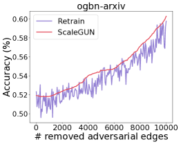
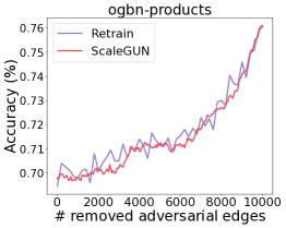
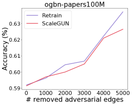
Figure 6: Comparison of unlearning efficacy for deep model: Model accuracy v.s. the number of removed adversarial edges.

Table 12: Deleted Data Replay Test: The ratio of incorrectly labeled nodes, $r_{d},r_{a}$, after unlearning.

Model	$r_{d}=\frac{|\{i\in\mathcal{V}_{d}|\hat{y}_{i}=c\}|}{|\mathcal{V}_{d}|}$ (%, $\downarrow$)			$r_{a}=\frac{|\{i\in\mathcal{V}|\hat{y}_{i}=c\}|}{|\mathcal{V}|}$ (%, $\downarrow$)
	Cora	ogbn-arxiv	ogbn-products	Cora	ogbn-arxiv	ogbn-products
Origin	100	90.72$\pm$4.19	100	52.13$\pm$3.35	1.01$\pm$0.07	45.59$\pm$13.90
Retrain	0	0	0	0	0	0
CGU	0	0	0	0.09$\pm$0.03	0	0
ScaleGUN	0	0	0	0.08$\pm$0.01	0	0

Deleted Data Replay Test (DDRT). We follow GraphEditor Cong and Mahdavi to conduct DDRT on Cora, ogbn-arxiv, and ogbn-products for linear models in Table  12. First, we choose a set of nodes $\mathcal{V}_{d}$ to be unlearned from the training set and add 100-dimensional binary features to the original node features. For nodes in $\mathcal{V}_{d}$, these additional features are set to 1; for other nodes, they are set to 0. The labels of nodes in $\mathcal{V}_{d}$ are assigned to a new class $c$. An effective unlearning method is expected not to predict the unlearned nodes as class $c$ after unlearning $\mathcal{V}_{d}$, meaning that $\hat{y}_{i}\neq c$ for $i\in\mathcal{V}_{d}$. We report the ratio of incorrectly labeled nodes $r_{d}=\frac{|\{i\in\mathcal{V}_{d}|\hat{y}_{i}=c\}|}{|\mathcal{V}_{d}|}$ in the original model (which does not unlearn any nodes) and target models after unlearning. We set $|\mathcal{V}_{d}|=100,125,50000$

Table 13: MIA: The ratio of the presence probability of the unlearned nodes between the original model and target models after unlearning.

Target model	Cora ($\uparrow$)	ogbn-arxiv ($\uparrow$)
Retrain	1.698$\pm$0.21	1.232$\pm$0.388
CGU	1.526$\pm$0.120	1.231$\pm$0.388
ScaleGUN	1.524$\pm$0.130	1.232$\pm$0.388

for Cora, ogbn-arxiv, and ogbn-products, respectively. We also report $r_{a}=\frac{|\{i\in\mathcal{V}|\hat{y}_{i}=c\}|}{|\mathcal{V}|}$ to assess whether the impact of the unlearned nodes is completely removed from the graph. The results show that ScaleGUN successfully removes the impact of the unlearned nodes, with only a slight discrepancy compared to retraining.

Membership Inference Attack (MIA). As noted in Chien et al. [2022b], MIA has distinct design goals from unlearning. Even after unlearning a training node, the attack model may still recognize the unlearned node in the training set if there are other similar training nodes. Nonetheless, we follow Chien et al. [2022b], Cheng et al. [2023] to conduct MIA Olatunji et al. [2021] on Cora and ogbn-arxiv in Table 13. The core idea is that if the target model effectively unlearns a training node, the MI attacker will determine that the node is not present in the training set, i.e., the presence probability of the unlearned nodes decreases. We remove 100 training nodes from Cora and 125 from ogbn-arxiv. We then report the ratio of the presence probability of these unlearned nodes between the original model (which does not unlearn any nodes) and target models after unlearning. A reported ratio greater than $1.0$ indicates that the target model has successfully removed some information about the unlearned nodes, with higher values indicating better performance. Table 13 indicates that ScaleGUN offers privacy-preserving performance comparable to retraining in the context of MIA.

C.5 Apply ScaleGUN to spectral GNNs.

Besides decoupled GNNs that incorporate MLPs, ScaleGUN can also be applied to spectral GNNs Chien et al. [2020], Koyejo et al. [2022], which are a significant subset of existing GNN models and have shown

Table 14: Test accuracy (%), total unlearning cost (s), and propagation cost (s) per batch edge removal using ChebNetII as the backbone on ogbn-arxiv.

	Retrain	ScaleGUN
0	71.99	71.99
25	72.08	71.98
50	72.01	71.98
75	71.8	71.96
100	72.3	71.94
125	71.79	71.93
Prop	14.96	3.13
Total	58.51	5.84

superior performance in many popular benchmarks. For example, ChebNetII Koyejo et al. [2022] can be expressed as ${Y}=f_{\theta}(Z),Z=\sum_{k=0}^{K}w_{k}T_{k}(\hat{L})X$ when applied to large graphs, where $T_{k}$ are the Chebyshev polynomials, $f_{\theta}$ is a MLP and $w_{k}$ are learnable parameters. We can maintain $T_{k}(\hat{L})X$ using the lazy local framework and perform unlearning on $f_{\theta}$ and $w_{k}$, similar to that of Table 2. Table 14 demonstrated the unlearning results using ChebNetII as the backbone on ogbn-arxiv, mirroring the unlearning settings with Table 1. This suggests that ScaleGUN can achieve competitive performance when no certified guarantees are required.

Licenses of the datasets. Ogbn-arxiv and ogbn-papers100M are both under the ODC-BY license. Cora, Citeseer, Photo, and ogbn-products are under the CC0 1.0 license, Creative Commons license, Open Data Commons Attribution License, and Amazon license, respectively.

Appendix D Details of Lazy Local Propagation Framework

D.1 Differences between ScaleGUN and existing dynamic propagation methods

Existing dynamic propagation methods focus on the PPR-based propagation scheme, while ScaleGUN adopts the GPR-based one. Note that these dynamic propagation methods based on PPR cannot be straightforwardly transformed to accommodate GPR. Specifically, PPR-based methods can simply maintain a reserve vector $\boldsymbol{q}$ and a residue vector $\boldsymbol{r}$. In contrast, GPR-based propagation requires $\boldsymbol{q}^{(\ell)}$ and $\boldsymbol{r}^{(\ell)}$ for each level $\ell$. This difference also impacts the theoretical analysis of correctness and time complexity. Therefore, we have developed tailored algorithms and conducted a comprehensive theoretical analysis of the GPR-based scheme.

Choosing GPR enhances the generalizability of our framework. Specifically, our framework computes the embedding $\mathbf{Z}=\sum_{\ell=0}^{L}w_{\ell}\mathbf{P}^{\ell}\mathbf{X}$, wherein PPR, the weights $w_{\ell}$ are defined as $\alpha(1-\alpha)^{\ell}$ with $\alpha$ being the decay factor and $L$ tending towards infinity. Such a formulation allows the theoretical underpinnings of ScaleGUN to be directly applicable to PPR-based models, illustrating the broader applicability of our approach. One could replace the propagation part in ScaleGUN with the existing dynamic PPR approaches and obtain a certifiable unlearning method for PPR-based models. Conversely, confining our analysis to PPR would notably limit the expansiveness of our results.

Limitations of InstantGNN to achieve certified unlearning. InstantGNN [Zheng et al., 2022] provides an incremental computation method for the graph embeddings of dynamic graphs, accommodating insertions/deletions of nodes/edges and modifications of node features. However, simply applying InstantGNN for unlearning does not lead to certified unlearning, as this requires a thorough analysis of the impact of approximation error on the certified unlearning guarantee. Certified unlearning mandates that the gradient residual norm on exact embeddings, i.e., $||\nabla L(w^{-},D^{\prime})||$, remains within the privacy limit, as detailed in Theorem 2.1. InstantGNN, which relies on approximate embeddings for training, lacks a theoretical analysis of $||\nabla L(w^{-},D^{\prime})||$. Whether InstantGNN retrains the model for each removal or employs an adaptive training strategy for better performance, it lacks solid theoretical backing. Thus, InstantGNN is considered a heuristic method without theoretical support.

D.2 Algorithms of Lazy Local Propagation Framework

Initial propagation. Algorithm 2 illustrates the pseudo-code of Forward Push on a graph $\mathcal{G}$ with $\mathbf{P}=\mathbf{A}\mathbf{D}^{-1}$ and $L$ propagation steps. Initially, we normalize $\mathbf{x}$ to ensure $\left\lVert\mathbf{D}^{\frac{1}{2}}\mathbf{x}\right\rVert_{1}\leq 1$, and let $\boldsymbol{q}^{(\ell)}=\boldsymbol{r}^{(\ell)}=\mathbf{0}$ for $0\leq\ell\leq L$, except for $\boldsymbol{r}^{(0)}=\mathbf{D}^{\frac{1}{2}}\mathbf{x}$ when $\ell=0$. After employing Algorithm 2, we obtain $\mathbf{\hat{z}}=\sum_{\ell=0}^{L}{w_{\ell}}\mathbf{D}^{-\frac{1}{2}}\boldsymbol{q}^{(\ell)}$ as the approximation of $\mathbf{z}$.

Input: Graph $\mathcal{G}$, level $L$, threshold $r_{\max}$, and initialized $\{\boldsymbol{q}^{(\ell)},\boldsymbol{r}^{(\ell)}\},0\leq\ell\leq L$

Output: New estimated vectors $\{\boldsymbol{q}^{(\ell)},\boldsymbol{r}^{(\ell)}\}$

1 for $\ell$ from 0 to $L-1$ do

2       for $u\in V$ with $|\boldsymbol{r}^{(\ell)}(u)|>r_{\max}$  do

3             for each $v\in\mathcal{N}(u)$  do

4                   $\boldsymbol{r}^{(\ell+1)}(v)+=\frac{\boldsymbol{r}^{(\ell)}(u)}{d(u)}$;

5                  

6            $\boldsymbol{q}^{(\ell)}(u)+=\boldsymbol{r}^{(\ell)}(u)\text{ and }\boldsymbol{r}^{(\ell)}(u)\leftarrow 0$ ;

7            

8      

9$\boldsymbol{q}^{(L)}\leftarrow\boldsymbol{q}^{(L)}+\boldsymbol{r}^{(L)}$ and $\boldsymbol{r}^{(L)}\leftarrow$ $\mathbf{0}^{n\times F}$;

return $\{\boldsymbol{q}^{(\ell)},\boldsymbol{r}^{(\ell)}\},0\leq\ell\leq L$

Algorithm 2 BasicProp

Input: Graph $\mathcal{G}$, level $L$, edge $e=(u,v)$ to be removed, threshold $r_{\text{max}}$, $\{w_{\ell}\}$ and $\{\boldsymbol{q}^{(\ell)},\boldsymbol{r}^{(\ell)}\}$, $0\leq\ell\leq L$

Output: $\mathbf{\hat{Z}}\in\mathbb{R}^{n}$

1 $\mathcal{G}^{\prime}\leftarrow$ delete $(u,v)$ from $\mathcal{G}$ ;

2 $\boldsymbol{r}^{(0)}(u)\leftarrow\boldsymbol{r}^{(0)}(u)+(d(u)^{\frac{1}{2}}-(d(u)+1)^{\frac{1}{2}})\mathbf{x}(u)$;

3 $\boldsymbol{r}^{(0)}(v)\leftarrow\boldsymbol{r}^{(0)}(v)+(d(v)^{\frac{1}{2}}-(d(v)+1)^{\frac{1}{2}})\mathbf{x}(v)$;

4 for $\ell$ from $1$ to $L$ do

5       $\boldsymbol{r}^{(\ell)}{(u)}\leftarrow\boldsymbol{r}^{(\ell)}{(u)}-\frac{\boldsymbol{q}^{(\ell-1)}(v)}{d(v)+1}$;

6       for $w\in\mathcal{N}(u)$ do

7             $\boldsymbol{r}^{(\ell)}(w)\leftarrow\boldsymbol{r}^{(\ell)}(w)+\frac{\boldsymbol{q}^{(\ell-1)}(u)}{d(u)(d(u)+1)}$;

8            

9      $\boldsymbol{r}^{(\ell)}{(v)}\leftarrow\boldsymbol{r}^{(\ell)}{(v)}-\frac{\boldsymbol{q}^{(\ell-1)}(u)}{d(u)+1}$;

10       for $w\in\mathcal{N}(v)$ do

11             $\boldsymbol{r}^{(\ell)}(w)\leftarrow\boldsymbol{r}^{(\ell)}(w)+\frac{\boldsymbol{q}^{(\ell-1)}(v)}{d(v)(d(v)+1)}$;

12            

13      

14$\{\boldsymbol{q}^{(\ell)},\boldsymbol{r}^{(\ell)}\}\leftarrow{\sf BasicProp}(\mathcal{G}^{\prime},L,r_{\rm max},\{\boldsymbol{q}^{(\ell)},\boldsymbol{r}^{(\ell)}\})$;

return $\sum_{\ell=0}^{L}w_{\ell}\mathbf{D}^{-\frac{1}{2}}\boldsymbol{q}^{(\ell)}$

Algorithm 3 UpdateEmbeddingMatrix(EdgeRemoval)

Efficient Removal. Algorithm 3 details the update process for edge removal. Upon a removal request, we first adjust $\{\boldsymbol{r}^{(\ell)}\}$ locally for the affected nodes to maintain the invariant property. Post-adjustment, the invariant property is preserved across all nodes. Then, Algorithm 2 is invoked to reduce the error further and returns the updated $\mathbf{\hat{z}}$. Note that the degree of node $u$ and node $v$ is revised in Line 3.

Batch update. Inspired by Zheng et al. [2022], we introduce a parallel removal algorithm upon receiving a batch of removal requests. Specifically, we initially update the graph structure to reflect all removal requests and then compute the final adjustments for each affected node. Notably, the computation is conducted only once, thus significantly enhancing efficiency. We extend Algorithm 3 to accommodate batch-edge removal, simultaneously enabling parallel processing for multiple edges. The core concept involves adjusting both the reserves and residues for nodes impacted by the removal, deviating from Algorithm 3 where only the residues are modified. The benefit of altering the reserves is that only the reserves and residues for nodes $u$ and $v$ need updates when removing the edge $(u,v)$. Consequently, this allows the removal operations for all edges to be executed in parallel. Algorithm 4 details the batch update process for edge removal. Batch-node removal and batch-feature removal can be similarly implemented.

Input: Graph $\mathcal{G}$, level $L$, edges to be unlearned $S=\{e_{1},\cdots,e_{k}\}$, weight coefficients $w_{\ell}$, threshold $r_{\text{max}}$, $(\boldsymbol{q}^{(\ell)},\boldsymbol{r}^{(\ell)})$, $0\leq\ell\leq L$

Output: $\mathbf{\hat{Z}}\in\mathbb{R}^{n}$

1 Update $\mathcal{G}$ according to $S$, and let $\Delta_{u}$ be the number of removed neighbors of node $u$;

2 $V_{a}\leftarrow\{u\mid\text{the degree of node }u\text{ has changed}\}$;

3 parallel for $u\in V_{a}$ do

4      

5      $\boldsymbol{q}^{(0)}(u)\leftarrow\frac{d(u)}{d(u)+\Delta(u)}\boldsymbol{q}^{(0)}(u)$;

6       $\boldsymbol{r}^{(0)}(u)\leftarrow d(u)^{\frac{1}{2}}\mathbf{x}(u)-\boldsymbol{q}^{(0)}(u)$;

7      

8for $\ell$ from $1$ to $L$ do

9       parallel for $u\in V_{a}$ do

10             $\boldsymbol{q}^{(\ell)}(u)\leftarrow\frac{d(u)}{d(u)+\Delta(u)}\boldsymbol{q}^{(\ell)}(u)$;

11             $\boldsymbol{r}^{(\ell)}(u)\leftarrow\boldsymbol{r}^{(\ell)}(u)+\frac{\Delta(u)}{d(u)}\boldsymbol{q}^{(\ell)}(u)$;

12             for each $v\in$ $\{$removed neighbors of node $u\}$ do

13                   $\boldsymbol{r}^{(\ell)}(u)\leftarrow\boldsymbol{r}^{(\ell)}(u)-\frac{\boldsymbol{q}^{(\ell-1)}(v)}{d(v)}$;

14                  

15            

16      

17$\{\boldsymbol{q}^{(\ell)},\boldsymbol{r}^{(\ell)}\}\leftarrow{\sf BasicProp}(\mathcal{G}^{\prime},L,r_{\rm max},\{w_{\ell}\},\{\boldsymbol{q}^{(\ell)},\boldsymbol{r}^{(\ell)}\})$;

return $\sum_{\ell=0}^{L}w_{\ell}\mathbf{D}^{-\frac{1}{2}}\boldsymbol{q}^{(\ell)}$

Algorithm 4 BatchUpdate(EdgeRemoval)

D.3 Theoretical Analysis of Lazy Local Propagation Framework

Denote $\{\Delta\boldsymbol{r}^{(\ell)}\}$ as the adjustments to residues before invoking Forward Push (Algorithm 2) for further reducing the error. For instance, we have $\Delta\boldsymbol{r}^{(\ell)}(u)=\frac{\boldsymbol{q}^{(\ell-1)}(v)}{d(v)+1}$ for $\ell>0$. Let $d$ be the average degree of the graph. We introduce the following theorems regarding the time complexity of our lazy local propagation framework.

Theorem D.1 (Initialization Cost, Update Cost, and Total Cost).

Let $\mathbf{\hat{z}}_{0}$ be the initial embedding vector generated from scratch. $\mathbf{\hat{z}}_{i}$ and $\{\boldsymbol{r}^{(\ell)}_{i}\}$ represents the approximate embedding vector and the residues after the $i$-th removal, respectively. Each embedding vector $\mathbf{\hat{z}}_{i}$ satisfies Lemma 3.1. Given the threshold $r_{\max}$, the cost of generating $\mathbf{\hat{z}}_{0}$ from scratch is $O\left(\left(L-\sum_{\ell=0}^{L-1}(L-\ell)\left\lVert\boldsymbol{r}^{(\ell)}_{0}\right\rVert_{1}\right)\cdot\frac{d}{r_{\max}}\right).$ The cost for updating $\mathbf{\hat{z}}_{i-1}$ and $\{\boldsymbol{r}^{(\ell)}_{i-1}\}$ to generate $\mathbf{\hat{z}}_{i}$ is

$$O\left(d+\frac{d}{r_{\max}}\cdot\sum_{\ell=0}^{L-1}(L-\ell)\left(\left\lVert{r}_{i-1}^{(\ell)}\right\rVert_{1}+\left\lVert\Delta\boldsymbol{r}^{(\ell)}_{i}\right\rVert_{1}-\left\lVert{r}_{i}^{(\ell)}\right\rVert_{1}\right)\right),$$

where $\{\Delta\boldsymbol{r}^{(\ell)}_{i}\}$ represent the adjustments of residues for the $i$-th removal. For a sequence of $K$ removal requests, the total cost of initialization and $K$ removals is

$$O\left(\frac{Ld}{r_{\max}}+Kd+\sum_{i=1}^{K}\sum_{\ell=0}^{L-1}\left\lVert\Delta\boldsymbol{r}^{(\ell)}_{i}\right\rVert_{1}\frac{Ld}{r_{\max}}\right).$$

Appendix E Proofs of Theoretical Results

Notations for proofs. For the sake of readability, we use $l(\mathbf{Z},\mathbf{w},i)$ to denote $l(\mathbf{e}_{i}^{\top}\mathbf{Z}\mathbf{w},\mathbf{e}_{i}^{\top}Y)$. $\mathbf{Z}_{i}$ represents the embedding column vector of node $i$. When referring to the embedding row vector of $\mathbf{Z}$, we use $\mathbf{e}_{i}^{\top}\mathbf{Z}$. $\mathbf{Z}_{ij}$ denotes the term at the $i$-th row and the $j$-th column of $\mathbf{Z}$. $\left\lvert{\bf v}\right\rvert$ represents the vector with the absolute value of each element in vector $\bf v$.

E.1 Proof of Equation (1) and Lemma 3.2

Equation (1) is presented as follows:

$$\mathbf{z}=\sum_{\ell=0}^{L}{w_{\ell}}\mathbf{D}^{-\frac{1}{2}}\left(\boldsymbol{q}^{(\ell)}+\sum_{t=0}^{\ell}(\mathbf{A}\mathbf{D}^{-1})^{\ell-t}\boldsymbol{r}^{(t)}\right).$$

Lemma.

For each feature vector $\mathbf{x}$, the reserve vectors $\{\boldsymbol{q}^{(\ell)}\}$ and the residue vectors $\{\boldsymbol{r}^{(\ell)}\}$ satisfy the following invariant property during the propagation process:

$$\left\{\begin{aligned} &\boldsymbol{q}^{(\ell)}(u)+\boldsymbol{r}^{(\ell)}(u)=\mathbf{D}(u)^{\frac{1}{2}}\mathbf{x}(u),&\ell=0\\ &\boldsymbol{q}^{(\ell)}(u)+\boldsymbol{r}^{(\ell)}(u)=\sum_{t\in\mathcal{N}(u)}\frac{\boldsymbol{q}^{(\ell-1)}(t)}{d(t)},&0<\ell\leq L\\ \end{aligned}\right.$$

For simplicity, we reformulate the invariant into the vector form:

$$\left\{\begin{aligned} &\boldsymbol{q}^{(\ell)}+\boldsymbol{r}^{(\ell)}=\mathbf{D}^{\frac{1}{2}}\mathbf{x},&\ell=0\\ &\boldsymbol{q}^{(\ell)}(u)+\boldsymbol{r}^{(\ell)}(u)=\mathbf{A}\mathbf{D}^{-1}\boldsymbol{q}^{(\ell-1)},&0<\ell\leq L\\ \end{aligned}\right.$$ (3)

We prove that Equation (1) and Lemma 3.2 hold during the propagation process by induction. At the beginning of the propagation, we initialize $\boldsymbol{q}^{(\ell)}=\mathbf{0}$ for all $\ell$, $\boldsymbol{r}^{(0)}=\mathbf{D}^{\frac{1}{2}}\mathbf{x}$ and $\boldsymbol{r}^{(\ell)}=\mathbf{0}$ for all $\ell>1$. Therefore, Equation (3) and Equation (1) hold at the initial state. Consider the situation of level $0$. Since we set $\boldsymbol{r}^{(0)}(u)=0$ and $\boldsymbol{q}^{(0)}(u)=\boldsymbol{r}^{(0)}(u)$ once we push the residue $\boldsymbol{r}^{(\ell)}(u)$. The sum of $\boldsymbol{r}^{(0)}(u)$ and $\boldsymbol{q}^{(0)}(u)$ for any node $u$ remains unchanged during the propagation. Thus, Equation (3) holds for level $0$. Consider the situation of level $\ell>0$. Assuming that Equation (3) and Equation (1) holds after a specific push operation. Consider a push operation on node $u$ from level $k$ to level $k+1$, $0\leq k<L$. Let $y=\boldsymbol{r}^{(k)}(u)$, $\mathbf{e}_{u}$ is the one-hot vector with only $1$ at the node $u$ and $0$ elsewhere. According to Line 2 to 2 in Algorithm 2, the push operation can be described as follows:

$$\boldsymbol{r}^{\prime(k+1)} =\boldsymbol{r}^{(k+1)}+\mathbf{A}\mathbf{D}^{-1}\cdot y\mathbf{e}_{u}$$ (4)

$$\boldsymbol{q}^{\prime(k)} =\boldsymbol{q}^{(k)}+y\mathbf{e}_{u}$$

$$\boldsymbol{r}^{\prime(k)} =\boldsymbol{r}^{(k)}-y\mathbf{e}_{u}$$

Therefore, we have

$$\boldsymbol{q}^{\prime(k+1)}+\boldsymbol{r}^{\prime(k+1)} =\boldsymbol{q}^{(k+1)}+\boldsymbol{r}^{(k+1)}+\mathbf{A}\mathbf{D}^{-1}\cdot y\mathbf{e}_{u}$$

$$\mathbf{A}\mathbf{D}^{-1}\boldsymbol{q}^{\prime(k)} =\mathbf{A}\mathbf{D}^{-1}(\boldsymbol{q}^{(k)}+y\mathbf{e}_{u})$$

Note that $\boldsymbol{q}^{(k+1)}+\boldsymbol{r}^{(k+1)}=\mathbf{A}\mathbf{D}^{-1}\boldsymbol{q}^{(k)}$ is satistied before this push operation. Thus, $\boldsymbol{q}^{\prime(k+1)}+\boldsymbol{r}^{\prime(k+1)}=\mathbf{A}\mathbf{D}^{-1}\boldsymbol{q}^{\prime(k)}$, and thus Equation (3) holds after this push operation. For Equation (1), the right side of the equation is updated to:

$$\sum_{\ell}^{L}w_{\ell}\mathbf{D}^{-\frac{1}{2}}\left(\boldsymbol{q}^{\prime(\ell)}+\sum_{t=0}^{\ell}(\mathbf{A}\mathbf{D}^{-1})^{\ell-t}\boldsymbol{r}^{\prime(t)}\right).$$

Plugging the updated $\boldsymbol{q}^{\prime(k)},\boldsymbol{r}^{\prime(k)},\boldsymbol{r}^{\prime(k+1)}$ into the equation, we derive that Equation (1) holds after this push operation. This completes the proof of Equation (1) and Lemma 3.2.

E.2 Proof of Lemma 3.1

Lemma.

Given the threshold $r_{\max}$, the $L_{2}$-error between $\mathbf{z}$ and $\mathbf{\hat{z}}$ is bounded by

$$\left\lVert\mathbf{\hat{z}}-\mathbf{z}\right\rVert_{2}\leq\sqrt{n}Lr_{\max}.$$ (5)

Proof.

As stated in Equation (1), we have

$$\mathbf{z}-\mathbf{\hat{z}}=\sum_{\ell=0}^{L}{w_{\ell}}\mathbf{D}^{-\frac{1}{2}}\sum_{t=0}^{\ell}(\mathbf{A}\mathbf{D}^{-1})^{\ell-t}\boldsymbol{r}^{(t)}.$$

Since the largest eigenvalue of $\mathbf{A}\mathbf{D}^{-1}$ is no greater than $1$, we have $\left\lVert(\mathbf{A}\mathbf{D}^{-1})^{\ell}\right\rVert_{2}\leq 1$ for $\ell\geq 0$. $\mathbf{D}$ is a diagonal matrix, and $d(u)^{\frac{-1}{2}}$ is no greater than $1$ for all $u$. Thus, $\left\lVert\mathbf{D}^{-\frac{1}{2}}\right\rVert_{2}\leq 1$. Therefore, we have

$$\left\lVert\mathbf{\hat{z}}-\mathbf{z}\right\rVert =\left\lVert\sum_{\ell=0}^{L}{w_{\ell}}\mathbf{D}^{-\frac{1}{2}}\sum_{t=0}^{\ell}(\mathbf{A}\mathbf{D}^{-1})^{\ell-t}\boldsymbol{r}^{(t)}\right\rVert$$

$$\leq \sum_{\ell=0}^{L}\left\lvert{w_{\ell}}\right\rvert\sum_{t=0}^{\ell}\left\lVert\mathbf{D}^{-\frac{1}{2}}(\mathbf{A}\mathbf{D}^{-1})^{\ell-t}\boldsymbol{r}^{(t)}\right\rVert$$

$$\leq \sum_{\ell=0}^{L}\left\lvert{w_{\ell}}\right\rvert\sum_{t=0}^{\ell}\left\lVert\mathbf{D}^{-\frac{1}{2}}\right\rVert\left\lVert(\mathbf{A}\mathbf{D}^{-1})^{\ell-t}\right\rVert\left\lVert\boldsymbol{r}^{(t)}\right\rVert.$$

The norm of $\boldsymbol{r}^{(t)}$ can be derived as $\sqrt{n}r_{\max}$ since each item of $\boldsymbol{r}^{(t)}$ is no greater than $r_{\max}$. Given that $\sum_{\ell=0}^{L}\left\lvert w_{\ell}\right\rvert\leq 1$, we conclude that $\left\lVert\mathbf{\hat{z}}-\mathbf{z}\right\rVert_{2}\leq\sqrt{n}Lr_{\max}$. ∎

E.3 Proof of Theorem D.1

Proof.

First, consider the initialization cost for generating $\mathbf{\hat{z}}_{0}$. Recall that we have $\boldsymbol{r}^{(0)}=\mathbf{D}^{\frac{1}{2}}\mathbf{x}$ before we invoke Algorithm 2. In Algorithm 2, we push the residue $\boldsymbol{r}^{(\ell)}(u)$ of node $u$ to its neighbors whenever $\boldsymbol{r}^{(\ell)}(u)>r_{\max}$. Each node is pushed at most once at each level. Thus, for level $0$, there are at most $\left\lVert\mathbf{D}^{\frac{1}{2}}\mathbf{x}-\boldsymbol{r}^{(0)}_{0}\right\rVert_{1}/r_{\max}$ nodes with residues greater than $r_{\max}$, where $\boldsymbol{r}^{(0)}_{0}$ is the residues of level $0$ after the generation. The average cost for one push operation is $O(d)$, the average degree of the graph. Therefore, it costs at most $T^{(0)}=\left\lVert\mathbf{D}^{\frac{1}{2}}\mathbf{x}-\boldsymbol{r}^{(0)}_{0}\right\rVert_{1}d/r_{\max}$ time to finish the push operations for level $0$. In Algorithm 2, a total of $\boldsymbol{r}^{(\ell)}(u)$ will be added to the residues at the next level once we perform push on node $u$. Therefore, after the push operations for level $0$, $\left\lVert\boldsymbol{r}^{(1)}\right\rVert_{1}$ is no greater than $\left\lVert\mathbf{D}^{\frac{1}{2}}\mathbf{x}-\boldsymbol{r}^{(0)}_{0}\right\rVert_{1}$. Thus, the cost of the push operations at level $1$ satisfies that

$$T^{(1)}\leq \left(\left\lVert\mathbf{D}^{\frac{1}{2}}\mathbf{x}-\boldsymbol{r}^{(0)}_{0}\right\rVert_{1}-\left\lVert\boldsymbol{r}^{(1)}_{0}\right\rVert_{1}\right)\cdot\frac{d}{r_{\max}}$$

$$= T^{(0)}-\left\lVert\boldsymbol{r}^{(1)}_{0}\right\rVert_{1}\cdot\frac{d}{r_{\max}},$$

Similarly, the cost of the push operations at level $\ell$ is bounded by $T^{(\ell)}=T^{(\ell-1)}-\left\lVert\boldsymbol{r}^{(\ell)}_{0}\right\rVert_{1}\frac{d}{r_{\max}}$. Therefore, the total cost of generating $\mathbf{\hat{z}}$ is $O\left(\left(L-\sum_{\ell=0}^{L-1}(L-\ell)\left\lVert\boldsymbol{r}^{(\ell)}_{0}\right\rVert_{1}\right)\cdot\frac{d}{r_{\max}}\right)$.

Second, consider the update cost for a single removal. For ease of analysis, we design the following update procedure: First, we update the residues of the nodes whose degrees have changed at all levels, corresponding to Algorithm 3 Line 3-3. We denote the residues as $\{{r}_{\pm i}^{(\ell)}\}$ after the first step. Then, we push the non-negative residues for all levels. We denote the residues as $\{{r}_{-i}^{(\ell)}\}$ after pushing the non-negative residues. Finally, we push the negative residues at all levels, resulting in the approximate embedding vector $\mathbf{\hat{z}}_{i}$ and its residues $\{{r}_{i}^{(\ell)}\}$. The cost of the first step is $O(d(u)+d(v))=O(d)$. Denote the cost of the push operations at level $\ell$ as $T^{(\ell)}$, which contains the cost of pushing non-negative residues $T^{(\ell)}_{+}$ and the cost of pushing negative residues $T^{(\ell)}_{-}$.

Consider the cost of pushing non-negative residues. For level $0$, we have

$$T^{(0)}_{+}=\left\lVert{r}_{-i}^{(0)}-{r}_{\pm i}^{(0)}\right\rVert_{1}\cdot\frac{d}{r_{\max}}\leq\left(\left\lVert{r}_{\pm i}^{(0)}\right\rVert_{1}-\left\lVert{r}_{-i}^{(0)}\right\rVert_{1}\right)\cdot\frac{d}{r_{\max}}.$$

Note that the residues at level $1$ will be modified since the non-negative residues at level $0$ are pushed. Specifically, let the modification be $\tilde{r}^{(1)}$, that is, the residues of level $1$ of this time is ${r}_{\pm i}^{(1)}+\tilde{r}^{(1)}$. Thus, the cost of pushing non-negative residues at level $1$ is

$$T^{(1)}_{+} =\left\lVert{r}_{-i}^{(1)}-\left({r}_{\pm i}^{(1)}+\tilde{r}^{(1)}\right)\right\rVert_{1}\cdot\frac{d}{r_{\max}}$$

$$\leq\left(\left\lVert{r}_{\pm i}^{(1)}\right\rVert_{1}-\left\lVert{r}_{-i}^{(1)}\right\rVert_{1}\right)\cdot\frac{d}{r_{\max}}+\left\lVert\tilde{r}^{(1)}\right\rVert_{1}\cdot\frac{d}{r_{\max}}.$$

Note that $\left\lVert\tilde{r}^{(1)}\right\rVert_{1}$ is exactly the sum of the pushed residues from level $0$, which is no greater than $\left\lVert{r}_{\pm i}^{(0)}\right\rVert_{1}-\left\lVert{r}_{-i}^{(0)}\right\rVert_{1}$. Thus, we have

$$T^{(1)}_{+}\leq\left(\left\lVert{r}_{\pm i}^{(1)}\right\rVert_{1}-\left\lVert{r}_{-i}^{(1)}\right\rVert_{1}\right)\cdot\frac{d}{r_{\max}}+T_{+}^{(0)}.$$

Similarly, we have

$$T^{(\ell)}_{+}\leq\left(\left\lVert{r}_{\pm i}^{(\ell)}\right\rVert_{1}-\left\lVert{r}_{-i}^{(\ell)}\right\rVert_{1}\right)\cdot\frac{d}{r_{\max}}+T_{+}^{(\ell-1)}.$$

Therefore, we derive that

$$T_{+}\leq\sum_{\ell=0}^{L-1}T_{+}^{(\ell)} \leq\sum_{\ell=0}^{L-1}(L-\ell)\left(\left\lVert{r}_{\pm i}^{(\ell)}\right\rVert_{1}-\left\lVert{r}_{-i}^{(\ell)}\right\rVert_{1}\right)\cdot\frac{d}{r_{\max}}.$$ (6)

The cost of pushing negative residues is similar. We have

$$T^{(0)}_{-}=\left\lVert{r}_{i}^{(0)}-{r}_{-i}^{(0)}\right\rVert_{1}\cdot\frac{d}{r_{\max}}\leq\left(\left\lVert{r}_{-i}^{(0)}\right\rVert_{1}-\left\lVert{r}_{i}^{(0)}\right\rVert_{1}\right)\cdot\frac{d}{r_{\max}}.$$

Thus $T_{-}$ can be derived as

$$T_{-}\leq\sum_{\ell=0}^{L-1}T_{-}^{(\ell)} =\sum_{\ell=0}^{L-1}(L-\ell)\left(\left\lVert{r}_{-i}^{(\ell)}\right\rVert_{1}-\left\lVert{r}_{i}^{(\ell)}\right\rVert_{1}\right)\cdot\frac{d}{r_{\max}}.$$ (7)

Summing up Equation (6) and Equation (7), the $i$-th update costs can be derived as

$$T_{i}\leq 2d+\sum_{\ell=0}^{L-1}(L-\ell)\left(\left\lVert{r}_{\pm i}^{(\ell)}\right\rVert_{1}-\left\lVert{r}_{i}^{(\ell)}\right\rVert_{1}\right)\cdot\frac{d}{r_{\max}}$$

Recall that ${r}_{\pm i}^{(\ell)}$ can be derived from ${r}_{i-1}^{(\ell)}$ by the first step. Let ${r}_{\pm i}^{(\ell)}={r}_{i-1}^{(\ell)}+\Delta\boldsymbol{r}^{(\ell)}_{i}$. We can conclude that

$$T_{i}\leq O\left(d+\frac{d}{r_{\max}}\cdot\sum_{\ell=0}^{L-1}(L-\ell)\left(\left\lVert{r}_{i-1}^{(\ell)}\right\rVert_{1}+\left\lVert\Delta\boldsymbol{r}^{(\ell)}_{i}\right\rVert_{1}-\left\lVert{r}_{i}^{(\ell)}\right\rVert_{1}\right)\right).$$

Finally, consider the total cost for $K$ removals. The total cost is the sum of the initial and update costs for $K$ updates.

$$T= T_{\rm init}+\sum_{i=1}^{K}T_{i}$$

$$\leq \left(L\left\lVert\mathbf{D}^{\frac{1}{2}}\mathbf{x}\right\rVert_{1}-\sum_{\ell=0}^{L-1}(L-\ell)\left\lVert\boldsymbol{r}^{(\ell)}_{0}\right\rVert_{1}\right)\cdot\frac{d}{r_{\max}}$$

$$+\sum_{i=1}^{K}d+\sum_{i=1}^{K}\frac{d}{r_{\max}}\cdot\sum_{\ell=0}^{L-1}(L-\ell)\left(\left\lVert{r}_{i-1}^{(\ell)}\right\rVert_{1}+\left\lVert\Delta\boldsymbol{r}^{(\ell)}_{i}\right\rVert_{1}-\left\lVert{r}_{i}^{(\ell)}\right\rVert_{1}\right)$$

$$\leq L\left\lVert\mathbf{D}^{\frac{1}{2}}\mathbf{x}\right\rVert_{1}\frac{d}{r_{\max}}+Kd$$

$$+\sum_{i=1}^{K}\frac{d}{r_{\max}}\cdot\sum_{\ell=0}^{L-1}(L-\ell)\left\lVert\Delta\boldsymbol{r}^{(\ell)}_{i}\right\rVert_{1}-\sum_{\ell=0}^{L-1}(L-\ell)\left\lVert{r}_{i}^{(\ell)}\right\rVert_{1}$$

$$\stackrel{{\scriptstyle(a)}}{{\leq}} L\left\lVert\mathbf{D}^{\frac{1}{2}}\mathbf{x}\right\rVert_{1}\frac{d}{r_{\max}}+Kd+\sum_{i=1}^{K}L\sum_{\ell=0}^{L-1}\left\lVert\Delta\boldsymbol{r}^{(\ell)}_{i}\right\rVert_{1}\frac{d}{r_{\max}},$$

where we omit the $-\sum_{\ell=0}^{L-1}(L-\ell)\left\lVert{r}_{K}^{(\ell)}\right\rVert_{1}$ in (a). This completes the proof. ∎

E.4 Proof of Theorem 3.3

Theorem.

For a sequence of $m$ removal requests that remove all edges of the graph, the amortized cost per edge removal is $O\left(L^{2}d\right)$. For a sequence of $K$ random edge removals, the expected cost per edge removal is $O\left(L^{2}d\right)$.

With the help of Theorem D.1, we derive the proof of Theorem 3.3 as follows.

Proof.

Consider the amortized cost for $m$ removal requests. First, we observe that $\sum_{i=1}^{m}\left\lVert\Delta\boldsymbol{r}^{(0)}_{i}\right\rVert_{1}=\left\lVert\mathbf{D}^{\frac{1}{2}}_{0}\mathbf{x}\right\rVert_{1}$, where we denote the degree matrix of the initial graph as $\mathbf{D}_{0}$. To explain, $\left\lVert\Delta\boldsymbol{r}^{(0)}\right\rVert_{1}=((d(u)+1)^{\frac{1}{2}}-d(u)^{\frac{1}{2}})\left\lvert\mathbf{x}(u)\right\rvert+((d(v)+1)^{\frac{1}{2}}-d(v)^{\frac{1}{2}})\left\lvert\mathbf{x}(v)\right\rvert$ if we remove edge $(u,v)$, where $d(u)$ is the new degree of node $u$. All nodes have no edges at the end of the $m$ removals. Thus, the sum of $\left\lVert\Delta\boldsymbol{r}_{m}^{(0)}\right\rVert_{1}$ for the $m$ removals is $\left\lVert\mathbf{D}_{0}^{\frac{1}{2}}\mathbf{x}\right\rVert_{1}$. And we observe that $\left\lVert\Delta\boldsymbol{r}^{(\ell)}\right\rVert_{1}$ for $\ell>0$ is $O\left(\left\lVert\Delta\boldsymbol{r}^{(0)}\right\rVert_{1}\right)$ for each removal. First, we have $\left\lVert\Delta\boldsymbol{r}^{(\ell)}\right\rVert_{1}=\frac{2\left\lvert\boldsymbol{q}^{(\ell-1)}(u)\right\rvert}{d(u)+1}+\frac{2\left\lvert\boldsymbol{q}^{(\ell-1)}(v)\right\rvert}{d(v)+1}.$ Note that $\sum_{t=1}^{L}\left\lvert\boldsymbol{q}^{(t-1)}(u)\right\rvert\leq 1$ and $\left\lvert\mathbf{x}(u)\right\rvert\leq 1$ since $\mathbf{x}$ is normalized such that $\left\lVert\mathbf{D}^{\frac{1}{2}}\mathbf{x}\right\rVert_{1}\leq 1$. Thus, $\left\lVert\Delta\boldsymbol{r}^{(\ell)}\right\rVert_{1}\leq\frac{2}{d(u)+1}+\frac{2}{d(v)+1}$. On the other hand, since $(d(u)+1)^{\frac{1}{2}}-d(u)^{\frac{1}{2}}\leq\frac{1}{2\sqrt{d(u)}}$, we have $\left\lVert\Delta\boldsymbol{r}^{(0)}\right\rVert_{1}\leq\frac{1}{2\sqrt{d(u)}}+\frac{1}{2\sqrt{d(v)}}$ due to $\left\lvert\mathbf{x}(u)\right\rvert\leq 1$ for any node $u$. Therefore, $\left\lVert\Delta\boldsymbol{r}^{(\ell)}\right\rVert_{1}\leq 4\left\lVert\Delta\boldsymbol{r}^{(0)}\right\rVert_{1}$ for any removal and any $\ell>0$. Thus, the sum $\sum_{\ell=0}^{L-1}\left\lVert\Delta\boldsymbol{r}^{(\ell)}\right\rVert_{1}=O\left(L\left\lVert\Delta\boldsymbol{r}^{(0)}\right\rVert_{1}\right)$. Plugging the result into the total cost in Theorem D.1, the total cost for $m$ removals is

$$T =L\left\lVert\mathbf{D}^{\frac{1}{2}}\mathbf{x}\right\rVert_{1}\frac{d}{r_{\max}}+md+\sum_{i=1}^{m}L\sum_{\ell=0}^{L-1}\left\lVert\Delta\boldsymbol{r}^{(\ell)}_{i}\right\rVert_{1}\frac{d}{r_{\max}}$$

$$\leq L\left\lVert\mathbf{D}^{\frac{1}{2}}\mathbf{x}\right\rVert_{1}\frac{d}{r_{\max}}+md+O\left(\sum_{i=1}^{m}L^{2}\left\lVert\Delta\boldsymbol{r}^{(0)}_{i}\right\rVert_{1}\frac{d}{r_{\max}}\right)$$

$$\leq L\left\lVert\mathbf{D}^{\frac{1}{2}}\mathbf{x}\right\rVert_{1}\frac{d}{r_{\max}}+md+O\left(L^{2}\left\lVert\mathbf{D}^{\frac{1}{2}}\mathbf{x}\right\rVert_{1}\frac{d}{r_{\max}}\right)$$

We set $r_{\max}=1/\sqrt{n_{t}n}$ by the certified unlearning requirement, where $n_{t}$ represents the size of the training set. Thus, $r_{\max}\geq 1/n$. The amortized cost per edge removal is

$$\frac{T}{m}=O\left(\frac{1}{m}\cdot L^{2}\left\lVert\mathbf{D}^{\frac{1}{2}}\mathbf{x}\right\rVert_{1}dn\right).$$

Since we have $m\geq n$ and $\left\lVert\mathbf{D}^{\frac{1}{2}}\mathbf{x}\right\rVert_{1}\leq 1$, we conclude that the amortized cost is $O(L^{2}d)$.

Consider the expected cost for $K$ random edge removals. Each node has the same probability of being the endpoint of a removed edge. When removing $e=(u,v)$, the part induced by node $u$ in $\sum_{\ell=0}^{L-1}\left\lVert\Delta\boldsymbol{r}^{(\ell)}\right\rVert_{1}$ can be expressed as

$$S_{u}= \left((d(u)+1)^{\frac{1}{2}}-d(u)^{\frac{1}{2}}\right)\left\lvert\mathbf{x}(u)\right\rvert$$

$$+\sum_{t=1}^{L}\frac{\left\lvert\boldsymbol{q}^{(t-1)}(u)\right\rvert}{d(u)+1}+\sum_{w\in\mathcal{N}(u)}\frac{\left\lvert\boldsymbol{q}^{(t-1)}(u)\right\rvert}{d(u)(d(u)+1)}.$$

The first term $\left((d(u)+1)^{\frac{1}{2}}-d(u)^{\frac{1}{2}}\right)\left\lvert\mathbf{x}(u)\right\rvert$ is less than $\left\lvert\mathbf{x}(u)\right\rvert$ and the second term equals $\frac{2\left\lvert\boldsymbol{q}^{(t-1)}(u)\right\rvert}{d(u)+1}$. Therefore, the expected value of $S_{u}$ is

$$\mathrm{E}[S_{u}]=\frac{1}{n}\sum_{u\in V}S_{u}=\frac{1}{n}\sum_{u\in V}\left\lvert\mathbf{x}(u)\right\rvert+\frac{2}{n}\sum_{u\in V}\sum_{t=1}^{L}\frac{\left\lvert\boldsymbol{q}^{(t-1)}(u)\right\rvert}{d(u)+1}.$$

The first term is $O(\frac{1}{n})$ and $\sum_{u\in V}\left\lvert\boldsymbol{q}^{(t-1)}(u)\right\rvert$ in second term is less than $1$ for all level $t$ both due to the fact that $\left\lVert\mathbf{D}^{\frac{1}{2}}\mathbf{x}\right\rVert_{1}\leq 1$. Thus, the second term is less than $\frac{2L}{n}$. The expected value of $S_{u}$ is $O(\frac{1}{n})$. Therefore, for one edge removal, the expected value of $\sum_{\ell=0}^{L-1}\left\lVert\Delta\boldsymbol{r}^{(\ell)}\right\rVert_{1}$ is $O(\frac{1}{n})$. Note that we set $r_{\max}=O(1/\sqrt{n_{t}n})\geq 1/n$. Plugging the result into the total cost in Theorem D.1, the expected cost per edge removal is $O\left(L^{2}d\right)$. ∎

E.5 Proof of Theorem 4.2

Theorem.

Suppose that Assumption 4.1 holds and the feature of node $u$ is to be unlearned. If $\forall j\in[F]$, $\left\lVert\hat{\mathbf{Z}}\mathbf{e}_{j}-\mathbf{Z}\mathbf{e}_{j}\right\rVert\leq\epsilon_{1}$, we have $\left\lVert\nabla\mathcal{L}(\mathbf{w}^{-},\mathcal{D}^{\prime})\right\rVert$ is less than

$$\left(\frac{c\gamma_{1}}{\lambda}F+c_{1}\sqrt{F(n_{t}-1)}\right)\left(\epsilon_{1}+\frac{8{\gamma_{1}}F}{\lambda(n_{t}-1)}\cdot\sqrt{d(u)}\right).$$

For the sake of simplicity, the upper bound of $\left\lVert\mathbf{Z}\mathbf{e}_{j}-\mathbf{Z}^{\prime}\mathbf{e}_{j}\right\rVert$ for all $j\in[F]$ is denoted as $\epsilon_{2}$ in the following analysis. At the end of the proof, we will plug the bound in Lemma E.1 into the result. We also assume that node $u$ is the $n_{t}$-th node in the training. We state the following lemmas to support the proof.

Lemma E.1.

Suppose that the feature of node $u$ is to be removed. Then, we have $\left\lVert\mathbf{Z}\mathbf{e}_{j}-\mathbf{Z}^{\prime}\mathbf{e}_{j}\right\rVert\leq\sqrt{d(u)}$ for all $j\in[F]$.

Lemma E.2.

$\forall j\in[F]$, suppose that $\left\lVert\hat{\mathbf{Z}}\mathbf{e}_{j}-\mathbf{Z}\mathbf{e}_{j}\right\rVert\leq\epsilon_{1}$. We have $\left\lVert\sum_{i\in[n_{t}-1]}\left(\mathbf{\hat{Z}}_{i}-\mathbf{Z}_{i}\right)\right\rVert\leq\sqrt{F(n_{t}-1)}\epsilon_{1}$.

Lemma E.3.

$\forall j\in[F]$, suppose that $\left\lVert\mathbf{Z}^{\prime}\mathbf{e}_{j}-\mathbf{Z}\mathbf{e}_{j}\right\rVert\leq\epsilon_{2}$. We have $\left\lVert\sum_{i\in[n_{t}-1]}\left(\mathbf{Z}_{i}^{\prime}-\mathbf{Z}_{i}\right)\right\rVert\leq\sqrt{F(n_{t}-1)}\epsilon_{2}$.

Lemma E.4.

For the embedding vector $\mathbf{z}=\sum_{\ell=0}^{L}w_{\ell}\left(\mathbf{D}^{-\frac{1}{2}}\mathbf{A}\mathbf{D}^{-\frac{1}{2}}\right)^{\ell}\mathbf{x}$, where $\left\lVert\mathbf{x}\right\rVert\leq 1$ and $\sum_{\ell=0}^{L}w_{\ell}\leq 1$, we have $\left\lVert\mathbf{z}\right\rVert\leq 1$.

Proof.

We note that $\left\lVert\nabla\mathcal{L}(\mathbf{w}^{-},\mathcal{D}^{\prime})\right\rVert$ can be written as

$$\left\lVert\nabla\mathcal{L}(\mathbf{w}^{-},\mathcal{D}^{\prime})+\nabla\mathcal{L}(\mathbf{w}^{-},\hat{\mathcal{D}}^{\prime})-\nabla\mathcal{L}(\mathbf{w}^{-},\hat{\mathcal{D}}^{\prime})\right\rVert,$$

which is less than $\left\lVert\nabla\mathcal{L}(\mathbf{w}^{-},\mathcal{D}^{\prime})-\nabla\mathcal{L}(\mathbf{w}^{-},\hat{\mathcal{D}}^{\prime})\right\rVert+\left\lVert\nabla\mathcal{L}(\mathbf{w}^{-},\hat{\mathcal{D}}^{\prime})\right\rVert$ due to the Minkowski inequality.

We start with the term $\left\lVert\nabla\mathcal{L}(\mathbf{w}^{-},\mathcal{D}^{\prime})-\nabla\mathcal{L}(\mathbf{w}^{-},\hat{\mathcal{D}}^{\prime})\right\rVert$. Observe that

$$\left\lVert\nabla\mathcal{L}(\mathbf{w}^{-},\mathcal{D}^{\prime})-\nabla\mathcal{L}(\mathbf{w}^{-},\hat{\mathcal{D}}^{\prime})\right\rVert$$

$$= \left\lVert\sum_{i\in[n_{t}-1]}\left(\nabla l(\mathbf{Z}^{\prime},\mathbf{w}^{-},i)-\nabla l(\mathbf{\hat{Z}}^{\prime},\mathbf{w}^{-},i)\right)\right\rVert$$

$$= \left\lVert\sum_{i\in[n_{t}-1]}\left(l^{\prime}(\mathbf{Z}^{\prime},\mathbf{w}^{-},i)\mathbf{Z}^{\prime}_{i}-l^{\prime}(\mathbf{\hat{Z}}^{\prime},\mathbf{w}^{-},i)\mathbf{\hat{Z}}^{\prime}_{i}\right)\right\rVert$$

$$\stackrel{{\scriptstyle(c)}}{{\leq}} \Big{(}\Big{\lVert}\sum_{i\in[n_{t}-1]}\left(l^{\prime}(\mathbf{Z}^{\prime},\mathbf{w}^{-},i)\mathbf{Z}^{\prime}_{i}-l^{\prime}(\mathbf{\hat{Z}}^{\prime},\mathbf{w}^{-},i)\mathbf{Z}^{\prime}_{i}\right)\Big{\rVert}$$ (8)

$$+\Big{\lVert}\sum_{i\in[n_{t}-1]}\left(l^{\prime}(\mathbf{\hat{Z}}^{\prime},\mathbf{w}^{-},i)\mathbf{Z}^{\prime}_{i}-l^{\prime}(\mathbf{\hat{Z}}^{\prime},\mathbf{w}^{-},i)\mathbf{\hat{Z}}^{\prime}_{i}\right)\Big{\rVert}\Big{)}.$$ (9)

where the inequality (c) is due to the Minkowski inequality. Consider Term (8), we have

$$\left\lVert\sum_{i\in[n_{t}-1]}\left(l^{\prime}(\mathbf{Z}^{\prime},\mathbf{w}^{-},i)\mathbf{Z}^{\prime}_{i}-l^{\prime}(\mathbf{\hat{Z}}^{\prime},\mathbf{w}^{-},i)\mathbf{Z}^{\prime}_{i}\right)\right\rVert$$

$$= \left\lVert\sum_{i\in[n_{t}-1]}\left(l^{\prime}(\mathbf{Z}^{\prime},\mathbf{w}^{-},i)-l^{\prime}(\mathbf{\hat{Z}}^{\prime},\mathbf{w}^{-},i)\right)\mathbf{Z}^{\prime}_{i}\right\rVert$$

$$= \sqrt{\sum_{j\in[F]}\left(\sum_{i\in[n_{t}-1]}\left(l^{\prime}(\mathbf{Z}^{\prime},\mathbf{w}^{-},i)-l^{\prime}(\mathbf{\hat{Z}}^{\prime},\mathbf{w}^{-},i)\right)\mathbf{Z}_{ij}^{\prime}\right)^{2}}$$

$$\stackrel{{\scriptstyle(a)}}{{\leq}} \sqrt{\sum_{j\in[F]}\sum_{i\in[n_{t}-1]}(l^{\prime}(\mathbf{Z}^{\prime},\mathbf{w}^{-},i)-l^{\prime}(\mathbf{\hat{Z}}^{\prime},\mathbf{w}^{-},i))^{2}\sum_{i\in[n_{t}-1]}\mathbf{Z}_{ij}^{\prime 2}},$$ (10)

where $(a)$ is due to the Cauchy-Schwarz inequality. Recalling that $l^{\prime}$ is $\gamma_{1}$-Lipschitz as stated in the Assumption 4.1, we derive that

$$\sum_{i\in[n_{t}-1]}(l^{\prime}(\mathbf{Z}^{\prime},\mathbf{w}^{-},i)-l^{\prime}(\mathbf{\hat{Z}}^{\prime},\mathbf{w}^{-},i))^{2}$$

$$\leq \sum_{i\in[n_{t}-1]}\gamma_{1}^{2}\left\lVert\mathbf{e}_{i}^{\top}\mathbf{Z}^{\prime}\mathbf{w}^{-}-\mathbf{e}_{i}^{\top}\mathbf{\hat{Z}}^{\prime}\mathbf{w}^{-}\right\rVert^{2}$$

$$\leq \sum_{i\in[n_{t}-1]}\gamma_{1}^{2}\left\lVert\mathbf{e}_{i}^{\top}\mathbf{Z}^{\prime}-\mathbf{e}_{i}^{\top}\mathbf{\hat{Z}}^{\prime}\right\rVert^{2}\left\lVert\mathbf{w}^{-}\right\rVert^{2}$$

$$\leq \left\lVert\mathbf{w}^{-}\right\rVert^{2}\sum_{i\in[n_{t}-1]}\gamma_{1}^{2}\left\lVert\mathbf{e}_{i}^{\top}\mathbf{Z}^{\prime}-\mathbf{e}_{i}^{\top}\mathbf{\hat{Z}}^{\prime}\right\rVert^{2}$$

$$\stackrel{{\scriptstyle(a)}}{{\leq}} {\gamma_{1}^{2}}F\epsilon_{1}^{2}\left\lVert\mathbf{w}^{-}\right\rVert^{2}.$$ (11)

For inequality $(a)$, note that

$$\sum_{i\in[n_{t}-1]}\left\lVert\mathbf{e}_{i}^{\top}\mathbf{Z}^{\prime}-\mathbf{e}_{i}^{\top}\mathbf{\hat{Z}}^{\prime}\right\rVert^{2}\leq\sum_{j\in[F]}\left\lVert\mathbf{Z}^{\prime}\mathbf{e}_{j}-\mathbf{\hat{Z}}^{\prime}\mathbf{e}_{j}\right\rVert^{2}\leq F\epsilon_{1}^{2},$$

which follows from the assumption that $\left\lVert\mathbf{Z}^{\prime}\mathbf{e}_{j}-\mathbf{\hat{Z}}^{\prime}\mathbf{e}_{j}\right\rVert\leq\epsilon_{1}$ for all $j$. Since $\mathbf{w}^{-}=\mathbf{w}^{\star}+\hat{\mathbf{H}}_{\mathbf{w}^{\star}}^{-1}\Delta$, we have

$$\left\lVert\mathbf{w}^{-}\right\rVert=\left\lVert\mathbf{w}^{\star}+\hat{\mathbf{H}}_{\mathbf{w}^{\star}}^{-1}\Delta\right\rVert\leq\left\lVert\mathbf{w}^{\star}\right\rVert+\left\lVert\hat{\mathbf{H}}_{\mathbf{w}^{\star}}^{-1}\Delta\right\rVert.$$ (12)

Note that $\left\lVert\nabla\ell(\mathbf{e}_{i}^{\top}\mathbf{Z}\mathbf{w},\mathbf{e}_{i}^{\top}Y)\right\rVert\leq c$ holds as stated in the Assumption 4.1. Thus,

$$\left\lVert\mathbf{w}^{\star}\right\rVert=\frac{\left\lVert\sum_{i\in[n_{t}]}\nabla\ell(\mathbf{e}_{i}^{\top}\mathbf{\hat{Z}}\mathbf{w}^{-},\mathbf{e}_{i}^{\top}\mathbf{Y})\right\rVert}{\lambda n_{t}}\leq\frac{c}{\lambda}.$$ (13)

Also, following from Lemma E.4, we have $\sum_{j\in[F]}\sum_{i\in[n_{t}-1]}\mathbf{Z}_{ij}^{\prime 2}\leq F$. Plugging Inequality (11), Inequality (12) and Inequality (13) into Inequality (10), we have

$$\left\lVert\sum_{i\in[n_{t}-1]}\left(l^{\prime}(\mathbf{Z}^{\prime},\mathbf{w}^{-},i)\mathbf{Z}^{\prime}_{i}-l^{\prime}(\mathbf{\hat{Z}}^{\prime},\mathbf{w}^{-},i)\mathbf{Z}^{\prime}_{i}\right)\right\rVert\leq{\gamma_{1}}F\epsilon_{1}\left(\frac{c}{\lambda}+\left\lVert\hat{\mathbf{H}}_{\mathbf{w}^{\star}}^{-1}\Delta\right\rVert\right).$$

Next, considering Term (9), we have

$$\left\lVert\sum_{i\in[n_{t}-1]}\left(l^{\prime}(\mathbf{\hat{Z}}^{\prime},\mathbf{w}^{-},i)\mathbf{Z}^{\prime}_{i}-l^{\prime}(\mathbf{\hat{Z}}^{\prime},\mathbf{w}^{-},i)\mathbf{\hat{Z}}^{\prime}_{i}\right)\right\rVert$$

$$= \left\lVert\sum_{i\in[n_{t}-1]}l^{\prime}(\mathbf{\hat{Z}}^{\prime},\mathbf{w}^{-},i)\left(\mathbf{Z}^{\prime}_{i}-\mathbf{\hat{Z}}^{\prime}_{i}\right)\right\rVert$$

$$\stackrel{{\scriptstyle(a)}}{{\leq}} c_{1}\left\lVert\sum_{i\in[n_{t}-1]}\left(\mathbf{Z}^{\prime}_{i}-\mathbf{\hat{Z}}^{\prime}_{i}\right)\right\rVert$$

$$\stackrel{{\scriptstyle(b)}}{{\leq}} c_{1}\sqrt{F(n_{t}-1)}\epsilon_{1},$$

where Inequality $(a)$ is due to the assumption that $\ell^{\prime}\leq c_{1}$ and $(b)$ follows from Lemma E.2 by substituting $\mathcal{D}$ with $\mathcal{D}^{\prime}$. Therefore, we have

$$\left\lVert\nabla\mathcal{L}(\mathbf{w}^{-},\mathcal{D}^{\prime})-\nabla\mathcal{L}(\mathbf{w}^{-},\hat{\mathcal{D}}^{\prime})\right\rVert$$

$$\leq {\gamma_{1}}\epsilon_{1}F\left(\frac{c}{\lambda}+\left\lVert\hat{\mathbf{H}}_{\mathbf{w}^{\star}}^{-1}\Delta\right\rVert\right)+c_{1}\sqrt{F(n_{t}-1)}\epsilon_{1}.$$ (14)

Next, our focus shifts to analyzing $\left\lVert\nabla\mathcal{L}(\mathbf{w}^{-},\hat{\mathcal{D}}^{\prime})\right\rVert$. While our approach draws partial inspiration from the proof of Theorem 1 in Chien et al. [2022a], it significantly diverges due to the approximation involved in the embedding matrix. This necessitates a distinct analytical framework. Let $\hat{G}(\mathbf{w})=\nabla\mathcal{L}(\mathbf{w},\hat{\mathcal{D}}^{\prime})$. Note that $\hat{G}:\mathbb{R}^{d}\rightarrow\mathbb{R}^{d}$ is a vector-valued function. By Taylor’s Theorem, there exists some $\eta\in[0,1]$ such that:

$$\hat{G}\left(\mathbf{w}^{-}\right) =\hat{G}\left(\mathbf{w}^{\star}+\hat{\mathbf{H}}_{\mathbf{w}^{\star}}^{-1}\Delta\right)=\hat{G}\left(\mathbf{w}^{\star}\right)+\nabla\hat{G}\left(\mathbf{w}^{\star}+\eta\hat{\mathbf{H}}_{\mathbf{w}^{\star}}^{-1}\Delta\right)\hat{\mathbf{H}}_{\mathbf{w}^{\star}}^{-1}\Delta$$

$$=\hat{G}\left(\mathbf{w}^{\star}\right)+\hat{\mathbf{H}}_{\mathbf{w}_{\eta}}\hat{\mathbf{H}}_{\mathbf{w}^{\star}}^{-1}\Delta$$

$$=\hat{G}(\mathbf{w}^{\star})+\Delta+\hat{\mathbf{H}}_{\mathbf{w}_{\eta}}\hat{\mathbf{H}}_{\mathbf{w}^{\star}}^{-1}\Delta-\Delta$$

$$\stackrel{{\scriptstyle(a)}}{{=}}\hat{\mathbf{H}}_{\mathbf{w}_{\eta}}\hat{\mathbf{H}}_{\mathbf{w}^{\star}}^{-1}\Delta-\Delta$$

$$=(\hat{\mathbf{H}}_{\mathbf{w}_{\eta}}-\hat{\mathbf{H}}_{\mathbf{w}^{\star}})\hat{\mathbf{H}}_{\mathbf{w}^{\star}}^{-1}\Delta.$$ (15)

Here, we denote $\hat{\mathbf{H}}_{\mathbf{w}_{\eta}}=\nabla\hat{G}\left(\mathbf{w}^{\star}+\eta\hat{\mathbf{H}}_{\mathbf{w}^{\star}}^{-1}\Delta\right)$ with $\mathbf{w}_{\eta}=\mathbf{w}^{\star}+\eta\hat{\mathbf{H}}_{\mathbf{w}^{\star}}^{-1}\Delta$. Equality (a) is due to $\Delta=\nabla\mathcal{L}(\mathbf{w}^{\star},\hat{\mathcal{D}})-\nabla\mathcal{L}(\mathbf{w}^{\star},\hat{\mathcal{D}}^{\prime})$ and $\mathbf{w}^{\star}$ is the unique minimizer of $\mathcal{L}(\cdot,\hat{\mathcal{D}})$. This gives:

$$\left\lVert\hat{G}\left(\mathbf{w}^{-}\right)\right\rVert=\left\lVert(\hat{\mathbf{H}}_{\mathbf{w}_{\eta}}-\hat{\mathbf{H}}_{\mathbf{w}^{\star}})\hat{\mathbf{H}}_{\mathbf{w}^{\star}}^{-1}\Delta\right\rVert\leq\left\lVert(\hat{\mathbf{H}}_{\mathbf{w}_{\eta}}-\hat{\mathbf{H}}_{\mathbf{w}^{\star}})\right\rVert\left\lVert\hat{\mathbf{H}}_{\mathbf{w}^{\star}}^{-1}\Delta\right\rVert.$$

First, we consider the term $\left\lVert(\hat{\mathbf{H}}_{\mathbf{w}_{\eta}}-\hat{\mathbf{H}}_{\mathbf{w}^{\star}})\right\rVert$. Let $\tilde{\mathbf{Z}}$ consist of the first $n_{t}-1$ rows of $\mathbf{\hat{Z}}^{\prime}$, $\mathbf{D}_{1}={\rm diag}(l^{\prime\prime}(\mathbf{\hat{Z}}^{\prime},\mathbf{w}_{\eta},1),\cdots,l^{\prime\prime}(\mathbf{\hat{Z}}^{\prime},\mathbf{w}_{\eta},n_{t}-1))$ and $\mathbf{D}_{2}={\rm diag}(l^{\prime\prime}(\mathbf{\hat{Z}}^{\prime},\mathbf{w}^{\star},1),\cdots,l^{\prime\prime}(\mathbf{\hat{Z}}^{\prime},\mathbf{w}^{\star},n_{t}-1)).$ By the definition, we have

$$\left\lVert\hat{\mathbf{H}}_{\mathbf{w}_{\eta}}-\hat{\mathbf{H}}_{\mathbf{w}^{\star}}\right\rVert$$

$$= \left\lVert\nabla^{2}\mathcal{L}(\mathbf{w}_{\eta},\hat{\mathcal{D}}^{\prime})-\nabla^{2}\mathcal{L}(\mathbf{w}^{\star},\hat{\mathcal{D}}^{\prime})\right\rVert$$

$$= \left\lVert\tilde{\mathbf{Z}}^{\top}\mathbf{D}_{1}\tilde{\mathbf{Z}}-\tilde{\mathbf{Z}}^{\top}\mathbf{D}_{2}\tilde{\mathbf{Z}}\right\rVert$$

$$\leq \left\lVert\tilde{\mathbf{Z}}^{\top}\right\rVert\left\lVert\mathbf{D}_{1}-\mathbf{D}_{2}\right\rVert\left\lVert\tilde{\mathbf{Z}}\right\rVert.$$

Note that $\left\lVert\tilde{\mathbf{Z}}^{\top}\right\rVert\left\lVert\tilde{\mathbf{Z}}\right\rVert=\left\lVert\tilde{\mathbf{Z}}^{\top}\tilde{\mathbf{Z}}\right\rVert$, and the trace of $\tilde{\mathbf{Z}}^{\top}\tilde{\mathbf{Z}}$ has the following upper bound:

$${\bf tr}(\tilde{\mathbf{Z}}^{\top}\tilde{\mathbf{Z}})=\sum_{j\in[F]}\left\lVert\tilde{\mathbf{Z}}\mathbf{e}_{j}\right\rVert^{2}\leq\sum_{j\in[F]}\left(\left\lVert\mathbf{Z}\mathbf{e}_{j}\right\rVert+\left\lVert\mathbf{\hat{Z}}\mathbf{e}_{j}-\mathbf{Z}\mathbf{e}_{j}\right\rVert\right)^{2}\leq(1+\epsilon_{1})^{2}F.$$

Thus, we have $\left\lVert\tilde{\mathbf{Z}}^{\top}\tilde{\mathbf{Z}}\right\rVert\leq F(1+\epsilon_{1})^{2}$. Since $\mathbf{D}_{1}-\mathbf{D}_{2}$ is a diagonal matrix, its norm equals the maximum absolute value of its diagonal elements. Due to the assumption that $l^{\prime}$ is $\gamma_{1}$-Lipschitz, we have $l^{\prime\prime}(\mathbf{Z},\mathbf{w},i)\leq\gamma_{1}$ for any $\mathbf{Z},\mathbf{w},i$. Thus, $\left\lVert\mathbf{D}_{1}-\mathbf{D}_{2}\right\rVert$ is upper bounded by $\gamma_{1}$. Therefore, we have

$$\left\lVert\hat{\mathbf{H}}_{\mathbf{w}_{\eta}}-\hat{\mathbf{H}}_{\mathbf{w}^{\star}}\right\rVert\leq\gamma_{1}(1+\epsilon_{1})^{2}F.$$ (16)

Since $\mathcal{L}(\cdot,\hat{\mathcal{D}}^{\prime})$ is $\lambda(n_{t}-1)$-strongly convex, we have $\left\lVert\hat{\mathbf{H}}_{\mathbf{w}^{\star}}\right\rVert\geq\lambda(n_{t}-1)$, hence $\left\lVert\hat{\mathbf{H}}_{\mathbf{w}^{\star}}^{-1}\right\rVert\leq\frac{1}{\lambda(n_{t}-1)}$. Next, we focus on bounding $\Delta=\nabla\mathcal{L}(\mathbf{w}^{\star},\hat{\mathcal{D}})-\nabla\mathcal{L}(\mathbf{w}^{\star},\hat{\mathcal{D}}^{\prime})$. In the feature unlearning scenario, we have

$$\Delta=\lambda\mathbf{w}^{\star}+\nabla l(\mathbf{\hat{Z}},\mathbf{w}^{\star},n_{t})+\sum_{i\in[n_{t}-1]}\left(\nabla l(\mathbf{\hat{Z}},\mathbf{w}^{\star},i)-\nabla l(\mathbf{\hat{Z}}^{\prime},\mathbf{w}^{\star},i)\right).$$

By assumption that $\left\lVert\nabla l(\mathbf{Z},\mathbf{w},i)\right\rVert\leq c$ and the fact that $\left\lVert\mathbf{w}^{\star}\right\rVert\leq\frac{c}{\lambda}$, we have $\left\lVert\lambda\mathbf{w}^{\star}+\nabla l(\mathbf{\hat{Z}},\mathbf{w}^{\star},n_{t})\right\rVert\leq 2c$. For the last term, we derive that

$$\left\lVert\sum_{i\in[n_{t}-1]}\nabla l(\mathbf{\hat{Z}},\mathbf{w}^{\star},i)-\sum_{i\in[n_{t}-1]}\nabla l(\mathbf{\hat{Z}}^{\prime},\mathbf{w}^{\star},i)\right\rVert$$

$$= \left\lVert\sum_{i\in[n_{t}-1]}\left(l^{\prime}(\mathbf{\hat{Z}},\mathbf{w}^{\star},i)\mathbf{\hat{Z}}_{i}-l^{\prime}(\mathbf{\hat{Z}}^{\prime},\mathbf{w}^{\star},i)\mathbf{\hat{Z}}^{\prime}_{i}\right)\right\rVert$$

$$\leq \left\lVert\sum_{i\in[n_{t}-1]}\left(l^{\prime}(\mathbf{\hat{Z}},\mathbf{w}^{\star},i)\mathbf{\hat{Z}}_{i}-l^{\prime}(\mathbf{\hat{Z}}^{\prime},\mathbf{w}^{\star},i)\mathbf{\hat{Z}}_{i}\right)\right\rVert$$ (17)

$$+\left\lVert\sum_{i\in[n_{t}-1]}\left(l^{\prime}(\mathbf{\hat{Z}}^{\prime},\mathbf{w}^{\star},i)\mathbf{\hat{Z}}_{i}-l^{\prime}(\mathbf{\hat{Z}}^{\prime},\mathbf{w}^{\star},i)\mathbf{\hat{Z}}^{\prime}_{i}\right)\right\rVert.$$ (18)

For Term (17), it can be bounded by

$$\left\lVert\sum_{i\in[n_{t}-1]}\left(l^{\prime}(\mathbf{\hat{Z}},\mathbf{w}^{\star},i)\mathbf{\hat{Z}}_{i}-l^{\prime}(\mathbf{\hat{Z}}^{\prime},\mathbf{w}^{\star},i)\mathbf{\hat{Z}}_{i}\right)\right\rVert$$

$$\leq \left\lVert\sum_{i\in[n_{t}-1]}\left(l^{\prime}(\mathbf{\hat{Z}},\mathbf{w}^{\star},i)-l^{\prime}(\mathbf{Z},\mathbf{w}^{\star},i)\right)\mathbf{\hat{Z}}_{i}\right\rVert$$

$$+\left\lVert\sum_{i\in[n_{t}-1]}\left(l^{\prime}(\mathbf{Z},\mathbf{w}^{\star},i)-l^{\prime}(\mathbf{Z}^{\prime},\mathbf{w}^{\star},i)\right)\mathbf{\hat{Z}}_{i}\right\rVert$$

$$+\left\lVert\sum_{i\in[n_{t}-1]}\left(l^{\prime}(\mathbf{Z}^{\prime},\mathbf{w}^{\star},i)-l^{\prime}(\mathbf{\hat{Z}}^{\prime},\mathbf{w}^{\star},i)\right)\mathbf{\hat{Z}}_{i}\right\rVert.$$

For the first term, similar to Term (8), we have

$$\left\lVert\sum_{i\in[n_{t}-1]}\left(l^{\prime}(\mathbf{\hat{Z}},\mathbf{w}^{\star},i)-l^{\prime}(\mathbf{Z},\mathbf{w}^{\star},i)\right)\mathbf{\hat{Z}}_{i}\right\rVert$$

$$\leq \sqrt{\sum_{j\in[F]}\sum_{i\in[n_{t}-1]}(l^{\prime}(\mathbf{\hat{Z}},\mathbf{w}^{\star},i)-l^{\prime}(\mathbf{Z},\mathbf{w}^{\star},i))^{2}\sum_{i\in[n_{t}-1]}\mathbf{\hat{Z}}_{ij}^{2}},$$

and

$$\sum_{i\in[n_{t}-1]}(l^{\prime}(\mathbf{\hat{Z}},\mathbf{w}^{\star},i)-l^{\prime}(\mathbf{Z},\mathbf{w}^{\star},i))^{2}$$

$$\leq \sum_{i\in[n_{t}-1]}\gamma_{1}^{2}\left\lVert\mathbf{e}_{i}^{\top}\mathbf{\hat{Z}}\mathbf{w}^{\star}-\mathbf{e}_{i}^{\top}\mathbf{Z}\mathbf{w}^{\star}\right\rVert^{2}$$

$$\leq \sum_{i\in[n_{t}-1]}\frac{c^{2}\gamma_{1}^{2}}{\lambda^{2}}\left\lVert\mathbf{e}_{i}^{\top}\mathbf{\hat{Z}}-\mathbf{e}_{i}^{\top}\mathbf{Z}\right\rVert^{2}$$

$${\leq} \frac{c^{2}\gamma_{1}^{2}}{\lambda^{2}}F\epsilon_{1}^{2}.$$

To derive the Frobenius norm of $\mathbf{\hat{Z}}$, $\sqrt{\sum_{j\in[F]}\sum_{i\in[n_{t}-1]}\mathbf{\hat{Z}}_{ij}^{2}}$, note that

$$\sum_{i\in[n_{t}-1]}\mathbf{\hat{Z}}_{ij}^{2} =\left\lVert\mathbf{\hat{Z}}\mathbf{e}_{j}\right\rVert^{2}\leq\left(\left\lVert\mathbf{Z}\mathbf{e}_{j}\right\rVert+\left\lVert\mathbf{\hat{Z}}\mathbf{e}_{j}-\mathbf{Z}\mathbf{e}_{j}\right\rVert\right)^{2}=(1+\epsilon_{1})^{2},$$

which implies that $\sqrt{\sum_{j\in[F]}\sum_{i\in[n_{t}-1]}\mathbf{\hat{Z}}_{ij}^{2}}\leq\sqrt{F}(1+\epsilon_{1})$. Thus, we have the first term bounded as

$$\left\lVert\sum_{i\in[n_{t}-1]}\left(l^{\prime}(\mathbf{\hat{Z}},\mathbf{w}^{\star},i)-l^{\prime}(\mathbf{Z},\mathbf{w}^{\star},i)\right)\mathbf{\hat{Z}}_{i}\right\rVert\leq\frac{c\gamma_{1}}{\lambda}F\epsilon_{1}(1+\epsilon_{1}).$$

The third term is the same as the first term, except that the embedding matrix is replaced by the updated one. Thus, we have

$$\left\lVert\sum_{i\in[n_{t}-1]}\left(l^{\prime}(\mathbf{Z}^{\prime},\mathbf{w}^{\star},i)-l^{\prime}(\mathbf{\hat{Z}}^{\prime},\mathbf{w}^{\star},i)\right)\mathbf{\hat{Z}}_{i}\right\rVert\leq\frac{c\gamma_{1}}{\lambda}F\epsilon_{1}(1+\epsilon_{1}).$$

The second term can be derived similarly,

$$\sum_{i\in[n_{t}-1]}(l^{\prime}(\mathbf{Z},\mathbf{w}^{\star},i)-l^{\prime}(\mathbf{Z}^{\prime},\mathbf{w}^{\star},i))^{2}$$

$$\leq \sum_{i\in[n_{t}-1]}\frac{c^{2}\gamma_{1}^{2}}{\lambda^{2}}\left\lVert\mathbf{e}_{i}^{\top}\mathbf{Z}-\mathbf{e}_{i}^{\top}\mathbf{Z}^{\prime}\right\rVert^{2}.$$

According to Lemma E.3, we derive that

$$\sum_{i\in[n_{t}-1]}(l^{\prime}(\mathbf{Z},\mathbf{w}^{\star},i)-l^{\prime}(\mathbf{Z}^{\prime},\mathbf{w}^{\star},i))^{2}\leq\frac{c^{2}\gamma_{1}^{2}}{\lambda^{2}}F\epsilon_{2}^{2}.$$

Therefore, the second term can be bounded as

$$\left\lVert\sum_{i\in[n_{t}-1]}\left(l^{\prime}(\mathbf{Z},\mathbf{w}^{\star},i)-l^{\prime}(\mathbf{Z}^{\prime},\mathbf{w}^{\star},i)\right)\mathbf{\hat{Z}}_{i}\right\rVert\leq\frac{c\gamma_{1}}{\lambda}F\epsilon_{2}(1+\epsilon_{1}).$$

Plugging the above results into Term (17), we have

$$\left\lVert\sum_{i\in[n_{t}-1]}\nabla l(\mathbf{\hat{Z}},\mathbf{w}^{\star},i)-\sum_{i\in[n_{t}-1]}\nabla l(\mathbf{\hat{Z}}^{\prime},\mathbf{w}^{\star},i)\right\rVert$$

$$\leq \frac{c\gamma_{1}}{\lambda}F(1+\epsilon_{1})(2\epsilon_{1}+\epsilon_{2}).$$

For Term (18), we have

$$\left\lVert\sum_{i\in[n_{t}-1]}\big{(}\ell^{\prime}(\mathbf{e}_{i}^{\top}\mathbf{\hat{Z}}^{\prime}\mathbf{w}^{\star},\mathbf{e}_{i}^{\top}\mathbf{Y})\mathbf{\hat{Z}}_{i}-\ell^{\prime}(\mathbf{e}_{i}^{\top}\mathbf{\hat{Z}}^{\prime}\mathbf{w}^{\star},\mathbf{e}_{i}^{\top}\mathbf{Y})\mathbf{\hat{Z}}^{\prime}_{i}\big{)}\right\rVert$$

$$= \left\lVert\sum_{i\in[n_{t}-1]}\ell^{\prime}(\mathbf{e}_{i}^{\top}\mathbf{\hat{Z}}^{\prime}\mathbf{w}^{\star},\mathbf{e}_{i}^{\top}\mathbf{Y})\big{(}\mathbf{\hat{Z}}_{i}-\mathbf{\hat{Z}}^{\prime}_{i}\big{)}\right\rVert$$

$$\stackrel{{\scriptstyle(a)}}{{\leq}} c_{1}\left\lVert\sum_{i\in[n_{t}-1]}\big{(}\mathbf{\hat{Z}}_{i}-\mathbf{\hat{Z}}^{\prime}_{i}\big{)}\right\rVert$$

$$\leq c_{1}\left\lVert\sum_{i\in[n_{t}-1]}\big{(}\mathbf{\hat{Z}}_{i}-\mathbf{Z}_{i}\big{)}\right\rVert$$

$$+c_{1}\left\lVert\sum_{i\in[n_{t}-1]}\big{(}\mathbf{Z}_{i}-\mathbf{Z}^{\prime}_{i}\big{)}\right\rVert+c_{1}\left\lVert\sum_{i\in[n_{t}-1]}\big{(}\mathbf{Z}^{\prime}_{i}-\mathbf{\hat{Z}}^{\prime}_{i}\big{)}\right\rVert,$$

where $(a)$ is due to the assumption that $\ell^{\prime}\leq c_{1}$. Plugging the results of Lemma E.2 and Lemma E.3 into the above inequality, we have $\left\lVert\sum_{i\in[n_{t}-1]}\big{(}\ell^{\prime}(\mathbf{e}_{i}^{\top}\mathbf{\hat{Z}}^{\prime}\mathbf{w}^{\star},\mathbf{e}_{i}^{\top}\mathbf{Y})\mathbf{\hat{Z}}_{i}-\ell^{\prime}(\mathbf{e}_{i}^{\top}\mathbf{\hat{Z}}^{\prime}\mathbf{w}^{\star},\mathbf{e}_{i}^{\top}\mathbf{Y})\mathbf{\hat{Z}}^{\prime}_{i}\big{)}\right\rVert\leq\\ c_{1}\sqrt{F(n_{t}-1)}(2\epsilon_{1}+\epsilon_{2}).$

Now we are ready to bound $\Delta$ for feature unlearning scenarios as follows:

$$\left\lVert\Delta\right\rVert=2c+\frac{c\gamma_{1}}{\lambda}F(1+\epsilon_{1})(2\epsilon_{1}+\epsilon_{2})+c_{1}\sqrt{F(n_{t}-1)}(2\epsilon_{1}+\epsilon_{2}).$$

Consequently, combining the results in Inequality (14) and Inequality (16), we have

$$\left\lVert\nabla\mathcal{L}(\mathbf{w}^{-},\mathcal{D}^{\prime})\right\rVert$$

$$\leq {\gamma_{1}}\epsilon_{1}F\left(\frac{c}{\lambda}+\left\lVert\hat{\mathbf{H}}_{\mathbf{w}^{\star}}^{-1}\Delta\right\rVert\right)+c_{1}\sqrt{F(n_{t}-1)}\epsilon_{1}+\gamma_{1}(1+\epsilon_{1})^{2}F\left\lVert\hat{\mathbf{H}}_{\mathbf{w}^{\star}}^{-1}\Delta\right\rVert$$

$$\leq \frac{c\gamma_{1}}{\lambda}F\epsilon_{1}+c_{1}\sqrt{F(n_{t}-1)}\epsilon_{1}+\left({\gamma_{1}}\epsilon_{1}F+\gamma_{1}(1+\epsilon_{1})^{2}F\right)\frac{1}{\lambda(n_{t}-1)}\Delta$$

$$\stackrel{{\scriptstyle(a)}}{{\leq}} \frac{c\gamma_{1}}{\lambda}F\epsilon_{1}+c_{1}\sqrt{F(n_{t}-1)}\epsilon_{1}+2{\gamma_{1}}F\frac{1}{\lambda(n_{t}-1)}\Delta.$$

Here, we omit the small term $(1+\epsilon_{1})$ for simplicity. Then $(a)$ follows from $\gamma_{1}\epsilon_{1}F\leq\gamma_{1}F$. Similarly, $\Delta$ can be derived as

$$\Delta\leq 2c+\left(\frac{c\gamma_{1}}{\lambda}F+c_{1}\sqrt{F(n_{t}-1)}\right)(2\epsilon_{1}+\epsilon_{2}).$$

Thus, we have

$$\left\lVert\nabla\mathcal{L}(\mathbf{w}^{-},\mathcal{D}^{\prime})\right\rVert$$

$$\leq \frac{c\gamma_{1}}{\lambda}F\epsilon_{1}+c_{1}\sqrt{F(n_{t}-1)}\epsilon_{1}+\frac{4c\gamma_{1}F}{\lambda(n_{t}-1)}$$

$$+\frac{2{\gamma_{1}}F}{\lambda(n_{t}-1)}\left(\frac{c\gamma_{1}}{\lambda}F+c_{1}\sqrt{F(n_{t}-1)}\right)(2\epsilon_{1}+\epsilon_{2})$$

$$\leq \frac{4c\gamma_{1}F}{\lambda(n_{t}-1)}+\left(\frac{c\gamma_{1}}{\lambda}F+c_{1}\sqrt{F(n_{t}-1)}\right)\left(\epsilon_{1}+\frac{2{\gamma_{1}}F}{\lambda(n_{t}-1)}(2\epsilon_{1}+\epsilon_{2})\right).$$

Plugging Lemma E.5 into the above inequality, we have

$$\left\lVert\nabla\mathcal{L}(\mathbf{w}^{-},\mathcal{D}^{\prime})\right\rVert$$

$$\leq \frac{4c\gamma_{1}F}{\lambda(n_{t}-1)}+\left(\frac{c\gamma_{1}}{\lambda}F+c_{1}\sqrt{F(n_{t}-1)}\right)\left(\epsilon_{1}+\frac{2{\gamma_{1}}F}{\lambda(n_{t}-1)}(2\epsilon_{1}+\sqrt{d(u)})\right).$$

Note that $c_{1}\sqrt{F(n_{t}-1)}\cdot\sqrt{d(u)}$ is much larger than $2c$, and thus $\frac{4c\gamma_{1}F}{\lambda(n_{t}-1)}$ is much smaller than $c_{1}\sqrt{F(n_{t}-1)}\cdot\frac{2\gamma_{1}F}{\lambda(n_{t}-1)}\cdot\sqrt{d(u)}$, which is include in the second term. Therefore, we omit $\frac{4c\gamma_{1}F}{\lambda(n_{t}-1)}$ and adjust by enlarging $\frac{2\gamma_{1}F}{\lambda(n_{t}-1)}$ to $\frac{4\gamma_{1}F}{\lambda(n_{t}-1)}$ for simplicity. Similarly, we omit the $2epsilon_{1}$ term and enlarge $\sqrt{d(u)}$ to $2\sqrt{d(u)}$. Finally, we have the upper bound of $\left\lVert\nabla\mathcal{L}(\mathbf{w}^{-},\mathcal{D}^{\prime})\right\rVert$ as

$$\left(\frac{c\gamma_{1}}{\lambda}F+c_{1}\sqrt{F(n_{t}-1)}\right)\left(\epsilon_{1}+\frac{8{\gamma_{1}}F}{\lambda(n_{t}-1)}\cdot\sqrt{d(u)}\right).$$

∎

E.6 Proof of Theorem 4.3

Theorem.

Suppose that Assumption 4.1 holds, and the edge $(u,v)$ is to be unlearned. If $\forall j\in[F]$, $\left\lVert\hat{\mathbf{Z}}\mathbf{e}_{j}-\mathbf{Z}\mathbf{e}_{j}\right\rVert\leq\epsilon_{1}$, we can bound $\left\lVert\nabla\mathcal{L}(\mathbf{w}^{-},\mathcal{D}^{\prime})\right\rVert$ by

$$\frac{4c\gamma_{1}F}{\lambda n_{t}}+\left(\frac{c\gamma_{1}}{\lambda}F+c_{1}\sqrt{Fn_{t}}\right)\left(\epsilon_{1}+\frac{4{\gamma_{1}}F}{\lambda n_{t}}(\epsilon_{1}+\frac{4}{\sqrt{d(u)}}+\frac{4}{\sqrt{d(v)}})\right).$$

In the proof of Theorem 4.3, we also denote the upper bound of $\left\lVert\mathbf{Z}\mathbf{e}_{j}-\mathbf{Z}^{\prime}\mathbf{e}_{j}\right\rVert$ for all $j\in[F]$ as $\epsilon_{2}$ before the conclusion is derived.

Lemma E.5.

Suppose that edge $e=(u,v)$ is to be removed. Then, we have $\left\lVert\mathbf{Z}\mathbf{e}_{j}-\mathbf{Z}^{\prime}\mathbf{e}_{j}\right\rVert\leq\frac{4}{\sqrt{d(u)}}+\frac{4}{\sqrt{d(v)}}$ for all $j\in[F]$.

Proof.

We can derive that $\left\lVert\sum_{i\in[n_{t}]}\left(\mathbf{\hat{Z}}_{i}-\mathbf{Z}_{i}\right)\right\rVert\leq\sqrt{Fn_{t}}\epsilon_{1}$ and $\left\lVert\sum_{i\in[n_{t}]}\left(\mathbf{Z}_{i}^{\prime}-\mathbf{Z}_{i}\right)\right\rVert\leq\sqrt{Fn_{t}}\epsilon_{2}$ by substituting $n_{t}-1$ by $n_{t}$ in the proofs of Lemma E.2 and Lemma E.3. Thus, by plugging the above results into the proof of Theorem 4.2, we derive that $\left\lVert\nabla\mathcal{L}(\mathbf{w}^{-},\mathcal{D}^{\prime})\right\rVert$ is less than

$${\gamma_{1}}\epsilon_{1}F\left(\frac{c}{\lambda}+\frac{1}{n_{t}}\left\lVert\Delta\right\rVert\right)+c_{1}\sqrt{Fn_{t}}\epsilon_{1}+\gamma_{1}(1+\epsilon_{1})^{2}F\left\lVert\frac{1}{n_{t}}\Delta\right\rVert$$

In the edge unlearning scenario, we have

$$\Delta=\sum_{i\in[n_{t}]}\left(\nabla l(\mathbf{\hat{Z}},\mathbf{w}^{\star},i)-\nabla l(\mathbf{\hat{Z}}^{\prime},\mathbf{w}^{\star},i)\right).$$

Similar to the analysis of the third term of $\Delta$ in the proof of Theorem 4.2, we have

$$\left\lVert\Delta\right\rVert\leq\frac{c\gamma_{1}}{\lambda}F(1+\epsilon_{1})(2\epsilon_{1}+\epsilon_{2})+c_{1}\sqrt{Fn_{t}}(2\epsilon_{1}+\epsilon_{2}).$$

Plugging Lemma E.5, we derive the upper bound of $\left\lVert\nabla\mathcal{L}(\mathbf{w}^{-},\mathcal{D}^{\prime})\right\rVert$ as

$$\frac{4c\gamma_{1}F}{\lambda n_{t}}+\left(\frac{c\gamma_{1}}{\lambda}F+c_{1}\sqrt{Fn_{t}}\right)\left(\epsilon_{1}+\frac{2{\gamma_{1}}F}{\lambda n_{t}}(2\epsilon_{1}+\frac{4}{\sqrt{d(u)}}+\frac{4}{\sqrt{d(v)}})\right).$$

∎

E.7 Proof of Theorem 4.4

Theorem.

Suppose that Assumption 4.1 holds and the feature of node $u$ is to be unlearned. If $\forall j\in[F]$, $\left\lVert\hat{\mathbf{Z}}\mathbf{e}_{j}-\mathbf{Z}\mathbf{e}_{j}\right\rVert\leq\epsilon_{1}$, we can bound $\left\lVert\nabla\mathcal{L}(\mathbf{w}^{-},\mathcal{D}^{\prime})\right\rVert$ by

$$\frac{4c\gamma_{1}F}{\lambda(n_{t}-1)}+\left(\frac{c\gamma_{1}}{\lambda}F+c_{1}\sqrt{F(n_{t}-1)}\right)\left(\epsilon_{1}+\frac{2{\gamma_{1}}F}{\lambda(n_{t}-1)}(2\epsilon_{1}+4\sqrt{d(u)}+\sum_{w\in\mathcal{N}(u)}\frac{4}{\sqrt{d(w)}})\right).$$

Lemma E.6.

Suppose that node $u$ is to be removed. Then, for all $j\in[F]$, it holds that:

$$\left\lVert\mathbf{Z}\mathbf{e}_{j}-\mathbf{Z}^{\prime}\mathbf{e}_{j}\right\rVert\leq 4\sqrt{d(u)}+\sum_{w\in\mathcal{N}(u)}\frac{4}{\sqrt{d(w)}}$$

Proof.

The node unlearning scenario is identical to the node feature unlearning scenario except for $\left\lVert\mathbf{Z}\mathbf{e}_{j}-\mathbf{Z}^{\prime}\mathbf{e}_{j}\right\rVert$. According to the proof of Theorem 4.2, we have

$$\left\lVert\nabla\mathcal{L}(\mathbf{w}^{-},\mathcal{D}^{\prime})\right\rVert\leq \frac{4c\gamma_{1}F}{\lambda(n_{t}-1)}+\left(\frac{c\gamma_{1}}{\lambda}F+c_{1}\sqrt{F(n_{t}-1)}\right)\left(\epsilon_{1}+2{\gamma_{1}}F\frac{1}{\lambda(n_{t}-1)}(2\epsilon_{1}+\epsilon_{2})\right).$$

Plugging Lemma E.6 into the above inequality, we derive the conclusion that $\left\lVert\mathbf{Z}\mathbf{e}_{j}-\mathbf{Z}^{\prime}\mathbf{e}_{j}\right\rVert$ is bounded by

$$\frac{4c\gamma_{1}F}{\lambda(n_{t}-1)}+\left(\frac{c\gamma_{1}}{\lambda}F+c_{1}\sqrt{F(n_{t}-1)}\right)\left(\epsilon_{1}+\frac{2{\gamma_{1}}F}{\lambda(n_{t}-1)}(2\epsilon_{1}+4\sqrt{d(u)}+\sum_{w\in\mathcal{N}(u)}\frac{4}{\sqrt{d(w)}})\right)$$

∎

E.8 Proof of Lemma E.1

Lemma.

Suppose that the feature of node $u$ is to be removed. Then, we have $\left\lVert\mathbf{Z}\mathbf{e}_{j}-\mathbf{Z}^{\prime}\mathbf{e}_{j}\right\rVert\leq\sqrt{d(u)}$ for all $j\in[F]$.

Proof.

Let $\mathbf{z}$ and $\mathbf{z}^{\prime}$ be the $j$-th column of $\mathbf{Z}$ and $\mathbf{Z}^{\prime}$, respectively. Correspondingly, let $\{\boldsymbol{r}^{(\ell)}\}$, $0\leq t\leq L$ are the residues of $\mathbf{z}$. And $\{\boldsymbol{r}^{\prime(\ell)}\}$ denotes the residues after the update operation for residues but before invoking Algorithm 2 to reduce the error further. Thus, $\mathbf{z}$ and $\mathbf{z}^{\prime}$ shares the same $\{\boldsymbol{q}^{(\ell)}\}$. First, we consider the difference between $\mathbf{z}$ and $\mathbf{z}^{\prime}$. We have

$$\mathbf{z}-\mathbf{z}^{\prime}=\sum_{\ell=0}^{L}{w_{\ell}}\sum_{t=0}^{\ell}\mathbf{D}^{-\frac{1}{2}}(\mathbf{A}\mathbf{D}^{-1})^{\ell-t}\left(\boldsymbol{r}^{(\ell)}-\boldsymbol{r}^{\prime(\ell)}\right).$$

Let $\Delta\boldsymbol{r}$ is the difference between $\boldsymbol{r}$ and $\boldsymbol{r}^{\prime}$, that is, $\Delta\boldsymbol{r}^{(\ell)}=\boldsymbol{r}^{\prime(\ell)}-\boldsymbol{r}^{(\ell)}$. Note that the node feature unlearning scenario does not revise the graph structure. Thus, the residues of the neighbors of $u$ and their neighbors are not updated. Since only $\boldsymbol{r}^{(0)}(u)$ is updated, we have

$$\left\lVert\mathbf{z}-\mathbf{z}^{\prime}\right\rVert_{1}\leq\sum_{\ell=0}^{L}\left\lvert w_{\ell}\right\rvert\mathbf{D}^{-\frac{1}{2}}(\mathbf{A}\mathbf{D}^{-1})^{\ell}\left\lvert\Delta\boldsymbol{r}^{(0)}(u)\right\rvert\mathbf{e}_{u}.$$

Since $\mathbf{A}\mathbf{D}^{-1}$ is a left stochastic matrix and $\mathbf{D}^{-\frac{1}{2}}$ will not increase the result, we derive that

$$S\leq\sum_{\ell=0}^{L}\left\lvert w_{\ell}\right\rvert\left\lvert\Delta\boldsymbol{r}^{(0)}(u)\right\rvert\mathbf{e}_{u}.$$

Due to the fact that $\sum_{\ell=0}^{L}\left\lvert w_{\ell}\right\rvert\leq 1$, it can be further bounded by $\left\lvert\Delta\boldsymbol{r}^{(0)}(u)\right\rvert$. As illustrated in Section 3, $\boldsymbol{r}^{\prime(0)}$ is modified to $-\boldsymbol{q}^{(0)}(u)$. Note that Equation (1) holds for all settings of $r_{\max}$. When $r_{\max}=0$, $\boldsymbol{r}^{(0)}$ is a zero vector. Combining Lemma 3.2, we have $\boldsymbol{q}^{(0)}(u)=d(u)^{\frac{1}{2}}\mathbf{x}(u)$. Therefore, $\left\lvert\Delta\boldsymbol{r}^{(0)}\right\rvert=d(u)^{\frac{1}{2}}\left\lvert\mathbf{x}(u)\right\rvert\leq d(u)^{\frac{1}{2}}$ due to the fact that $\mathbf{x}$ is normalized such that $\left\lVert\mathbf{D}^{\frac{1}{2}}\mathbf{x}\right\rVert_{1}\leq 1$. Consequently, we have $\left\lVert\mathbf{z}-\mathbf{z}^{\prime}\right\rVert_{1}\leq d(u)^{\frac{1}{2}}$. Thus, the $L2$-norm, which is always less than $L1$-norm, is bounded by $d(u)^{\frac{1}{2}}$, too. This holds for all $j\in[F]$, which completes the proof. ∎

E.9 Proof of Lemma E.5

Lemma.

Suppose that edge $e=(u,v)$ is to be removed. Then, we have $\left\lVert\mathbf{Z}\mathbf{e}_{j}-\mathbf{Z}^{\prime}\mathbf{e}_{j}\right\rVert\leq\frac{4}{\sqrt{d(u)}}+\frac{4}{\sqrt{d(v)}}$ for all $j\in[F]$.

Proof.

Similar to the proof of Lemma E.1, we have

$$\mathbf{z}-\mathbf{z}^{\prime}= \sum_{\ell=0}^{L}{w_{\ell}}\mathbf{D}^{-\frac{1}{2}}\left(\boldsymbol{q}^{(\ell)}+\sum_{t=0}^{\ell}(\mathbf{A}\mathbf{D}^{-1})^{\ell-t}\boldsymbol{r}^{(t)}\right)$$

$$-\sum_{\ell=0}^{L}{w_{\ell}}\mathbf{D}^{\prime-\frac{1}{2}}\left(\boldsymbol{q}^{(\ell)}+\sum_{t=0}^{\ell}(\mathbf{A}^{\prime}\mathbf{D}^{\prime-1})^{\ell-t}\boldsymbol{r}^{\prime(t)}\right),$$

where $\mathbf{A}^{\prime}$ and $\mathbf{D}^{\prime}$ are the adjacency matrix and the degree matrix of the graph after the edge removal, respectively. Let $\Delta\boldsymbol{r}$ is the difference between $\boldsymbol{r}$ and $\boldsymbol{r}^{\prime}$, that is, $\Delta\boldsymbol{r}^{(t)}=\boldsymbol{r}^{\prime(t)}-\boldsymbol{r}^{(t)}$. Then, we have

$$\mathbf{z}-\mathbf{z}^{\prime}$$

$$= \sum_{t=0}^{\ell}{w_{\ell}}\sum_{t=0}^{\ell}\left(\mathbf{D}^{-\frac{1}{2}}(\mathbf{A}\mathbf{D}^{-1})^{\ell-t}\boldsymbol{r}^{(t)}-\mathbf{D}^{\prime-\frac{1}{2}}(\mathbf{A}^{\prime}\mathbf{D}^{\prime-1})^{\ell-t}(\boldsymbol{r}^{(t)}+\Delta\boldsymbol{r}^{(t)})\right)$$

$$+\sum_{\ell=0}^{L}{w_{\ell}}\mathbf{D}^{-\frac{1}{2}}\boldsymbol{q}^{(\ell)}-\sum_{\ell=0}^{L}{w_{\ell}}\mathbf{D}^{\prime-\frac{1}{2}}\boldsymbol{q}^{(\ell)}$$

Note that the above equation holds under all settings of $r_{\max}$. Thus, we simply set $r_{\max}=0$ and then $\{\boldsymbol{r}^{(t)}\}$ are a zero vector for $0\leq t\leq L$. Therefore, it can be simplified as

$$\mathbf{z}-\mathbf{z}^{\prime}= \sum_{\ell=0}^{L}w_{\ell}\sum_{t=0}^{\ell}\mathbf{D}^{\prime-\frac{1}{2}}(\mathbf{A}^{\prime}\mathbf{D}^{\prime-1})^{\ell-t}\Delta\boldsymbol{r}^{(t)}$$

$$+\sum_{\ell=0}^{L}{w_{\ell}}\mathbf{D}^{-\frac{1}{2}}\boldsymbol{q}^{(\ell)}-\sum_{\ell=0}^{L}{w_{\ell}}\mathbf{D}^{\prime-\frac{1}{2}}\boldsymbol{q}^{(\ell)}$$

Consider the $L1$-norm of $\mathbf{z}-\mathbf{z}^{\prime}$. Note that the $L1$-norm of the first term is upper bounded by

$$S=\sum_{\ell=0}^{L}\left\lvert w_{\ell}\right\rvert\sum_{t=0}^{\ell}\sum_{i\in[n_{t}]}\mathbf{e}_{i}^{\top}\mathbf{D}^{\prime-\frac{1}{2}}(\mathbf{A}^{\prime}\mathbf{D}^{\prime-1})^{\ell-t}\left\lvert\Delta\boldsymbol{r}^{(t)}\right\rvert,$$

where $\left\lvert\Delta\boldsymbol{r}^{(t)}\right\rvert$ represents the vector with the absolute value of each element in $\Delta\boldsymbol{r}^{(t)}$. Since $\mathbf{A}^{\prime}\mathbf{D}^{\prime-1}$ is a left stochastic matrix and $\mathbf{D}^{\prime-\frac{1}{2}}$ will not increase the result, we derive that

$$S\leq\sum_{\ell=0}^{L}\left\lvert w_{\ell}\right\rvert\sum_{t=0}^{\ell}\sum_{i\in[n_{t}]}\mathbf{e}_{i}^{\top}\left\lvert\Delta\boldsymbol{r}^{(t)}\right\rvert.$$

Due to the fact that $\sum_{\ell=0}^{L}\left\lvert w_{\ell}\right\rvert\leq 1$, it can be further bounded by $\sum_{t=0}^{L}\sum_{i\in[n_{t}]}\mathbf{e}_{i}^{\top}\left\lvert\Delta\boldsymbol{r}^{(t)}\right\rvert$, that is, the sum of the absolute value of $\boldsymbol{r}^{(t)}$ for $0\leq t\leq L$. According to Algorithm 3, only the residues of node $u$, node $v$, and their neighbors will be updated. The sum induced by node $u$ can be written as

$$S_{u}= \left((d(u)+1)^{\frac{1}{2}}-d(u)^{\frac{1}{2}}\right)\left\lvert\mathbf{x}(u)\right\rvert$$

$$+\sum_{t=1}^{L}\frac{\left\lvert\boldsymbol{q}^{(t-1)}(u)\right\rvert}{d(u)+1}+\sum_{w\in\mathcal{N}(u)}\frac{\left\lvert\boldsymbol{q}^{(t-1)}(u)\right\rvert}{d(u)(d(u)+1)},$$

where the first term is the decreasement of $\boldsymbol{r}^{(0)}(u)$, the second term is the decreasement of the residues of $v$, and the third term is the increase of the residues of the neighbors of $u$. Note that $S_{u}\leq\frac{\left\lvert\mathbf{x}(u)\right\rvert}{2\sqrt{d(u)}}+\frac{2}{d(u)+1}\sum_{t=1}^{L}\left\lvert\boldsymbol{q}^{(t-1)}(u)\right\rvert$ due to the fact that $\left((d(u)+1)^{\frac{1}{2}}-d(u)^{\frac{1}{2}}\right)=\frac{1}{\sqrt{d(u)}+\sqrt{d(u)+1}}\leq\frac{1}{2\sqrt{d(u)}}$ and the new degree of $u$ is $d(u)$. Note that $\sum_{t=1}^{L}\left\lvert\boldsymbol{q}^{(t-1)}(u)\right\rvert\leq 1$ and $\left\lvert\mathbf{x}(u)\right\rvert\leq 1$ since $\mathbf{x}$ is normalized such that $\left\lVert\mathbf{D}^{\frac{1}{2}}\mathbf{x}\right\rVert_{1}\leq 1$. Thus, we have $S_{u}\leq\frac{1}{2\sqrt{d(u)}}+\frac{2}{d(u)+1}\leq\frac{3}{\sqrt{d(u)}}$. Similarly, the sum induced by node $v$ can be bounded by $\frac{1}{2\sqrt{d(v)}}+\frac{2}{d(v)+1}\leq\frac{3}{\sqrt{d(v)}}$.

Consider the second term. Only the degree of node $u$ and node $v$ is modified. Thus, we have

$$\left\lVert\sum_{\ell=0}^{L}{w_{\ell}}\mathbf{D}^{-\frac{1}{2}}\boldsymbol{q}^{(\ell)}-\sum_{\ell=0}^{L}{w_{\ell}}\mathbf{D}^{\prime-\frac{1}{2}}\boldsymbol{q}^{(\ell)}\right\rVert_{1}$$

$$= \sum_{\ell=0}^{L}\left\lvert w_{\ell}\right\rvert\left(d(u)^{-\frac{1}{2}}-(d(u)+1)^{-\frac{1}{2}}\right)\left\lvert\boldsymbol{q}^{(\ell)}(u)\right\rvert$$

$$+\sum_{\ell=0}^{L}\left\lvert w_{\ell}\right\rvert\left(d(v)^{-\frac{1}{2}}-(d(v)+1)^{-\frac{1}{2}}\right)\left\lvert\boldsymbol{q}^{(\ell)}(v)\right\rvert.$$

The term $\left(d(u)^{-\frac{1}{2}}-(d(u)+1)^{-\frac{1}{2}}\right)$ is less than $1/d(u)$. Thus, the second term is upper bounded by $\frac{1}{{d(u)}}+\frac{1}{{d(v)}}$. Sum up the two terms, we have $\left\lVert\mathbf{z}-\mathbf{z}^{\prime}\right\rVert_{1}\leq\frac{4}{\sqrt{d(u)}}+\frac{4}{\sqrt{d(v)}}$. Thus, the $L2$-norm, which is always less than $L1$-norm, is bounded by $\frac{4}{\sqrt{d(u)}}+\frac{4}{\sqrt{d(v)}}$, too. The lemma follows. ∎

E.10 Proof of Lemma E.6

Lemma.

Suppose that node $u$ is to be removed. Then, for all $j\in[F]$, it holds that:

$$\left\lVert\mathbf{Z}\mathbf{e}_{j}-\mathbf{Z}^{\prime}\mathbf{e}_{j}\right\rVert\leq 4\sqrt{d(u)}+\sum_{w\in\mathcal{N}(u)}\frac{4}{\sqrt{d(w)}}$$

Proof.

Removing a node is equivalent to removing all edges connected to the node. Thus, $\left\lVert\mathbf{Z}\mathbf{e}_{j}-\mathbf{Z}^{\prime}\mathbf{e}_{j}\right\rVert$ can be bounded by the sum of the bounds of removing all edges from node $u$. Drawing the result from Lemma E.5, the bound induced by removing one single edge can be bounded by $\frac{4}{\sqrt{d(u)}}+\frac{4}{\sqrt{d(w)}}$. Thus, the total sum is less than $4{\sqrt{d(u)}}+\sum_{w\in\mathcal{N}(u)}\frac{4}{\sqrt{d(w)}}$ by the triangle inequality. The lemma follows. ∎

E.11 Proof of Theorem 4.5

Theorem.

Let $\boldsymbol{R}^{(t)}\in\mathbb{R}^{n\times F}$ denote the residue matrix at level $t$, where the $j$-th column $\boldsymbol{R}^{(t)}\mathbf{e}_{j}$ represents the residue at level $t$ for the $j$-th feature vector. Let $\boldsymbol{R}$ be defined as the sum $\sum_{t=0}^{L}\boldsymbol{R}^{(t)}$. Consequently, we can establish the following data-dependent bound:

$$\left\lVert\nabla\mathcal{L}(\mathbf{w}^{-},\mathcal{D}^{\prime})\right\rVert\leq 2c_{1}\left\lVert\mathbf{1}^{\top}\boldsymbol{R}\right\rVert+\gamma_{2}\left\lVert\mathbf{\hat{Z}}^{\prime}\right\rVert\left\lVert\hat{\mathbf{H}}_{\mathbf{w}^{\star}}^{-1}\Delta\right\rVert\left\lVert\mathbf{\hat{Z}}^{\prime}\hat{\mathbf{H}}_{\mathbf{w}^{\star}}^{-1}\Delta\right\rVert.$$

Proof.

As demonstrated in the proof of Theorem 4.2, it is established that

$$\left\lVert\nabla\mathcal{L}(\mathbf{w}^{-},\mathcal{D}^{\prime})\right\rVert\leq\left\lVert\nabla\mathcal{L}(\mathbf{w}^{-},\mathcal{D}^{\prime})-\nabla\mathcal{L}(\mathbf{w}^{-},\hat{\mathcal{D}}^{\prime})\right\rVert+\left\lVert\nabla\mathcal{L}(\mathbf{w}^{-},\hat{\mathcal{D}}^{\prime})\right\rVert.$$

Initially, the data-dependent bound of the second term $\left\lVert\nabla\mathcal{L}(\mathbf{w}^{-},\hat{\mathcal{D}}^{\prime})\right\rVert$ can be inferred directly from Corollary 1 in Guo et al. [2019], by substituting $\mathcal{D}^{\prime}$ with $\hat{\mathcal{D}}^{\prime}$. This leads to the conclusion that $\left\lVert\nabla\mathcal{L}(\mathbf{w}^{-},\hat{\mathcal{D}}^{\prime})\right\rVert\leq\gamma_{2}\left\lVert\mathbf{\hat{Z}}^{\prime}\right\rVert\left\lVert\hat{\mathbf{H}}_{\mathbf{w}^{\star}}^{-1}\Delta\right\rVert\left\lVert\mathbf{\hat{Z}}^{\prime}\hat{\mathbf{H}}_{\mathbf{w}^{\star}}^{-1}\Delta\right\rVert$.

Focusing now on the first term.

$$\left\lVert\nabla\mathcal{L}(\mathbf{w}^{-},\mathcal{D}^{\prime})-\nabla\mathcal{L}(\mathbf{w}^{-},\hat{\mathcal{D}}^{\prime})\right\rVert$$

$$= \Big{\lVert}\sum_{i\in[n_{t}]}\left(l^{\prime}(\mathbf{Z}^{\prime},\mathbf{w}^{-},i)\mathbf{Z}^{\prime}_{i}-l^{\prime}(\mathbf{\hat{Z}}^{\prime},\mathbf{w}^{-},i)\mathbf{\hat{Z}}^{\prime}_{i}\right)\Big{\rVert}.$$

Since $l^{\prime}$ is bounded by $c_{1}$, we have

$$\Big{\lVert}\sum_{i\in[n_{t}]}\left(l^{\prime}(\mathbf{Z}^{\prime},\mathbf{w}^{-},i)\mathbf{Z}^{\prime}_{i}-l^{\prime}(\mathbf{\hat{Z}}^{\prime},\mathbf{w}^{-},i)\mathbf{\hat{Z}}^{\prime}_{i}\right)\Big{\rVert}$$

$$\leq 2c_{1}\Big{\lVert}\sum_{i\in[n_{t}]}\left(\mathbf{Z}^{\prime}_{i}-\mathbf{\hat{Z}}^{\prime}_{i}\right)\Big{\rVert}$$

$$= 2c_{1}\sqrt{\sum_{j\in[F]}\left(\sum_{i\in[n_{t}]}\mathbf{Z}^{\prime}_{ij}-\mathbf{\hat{Z}}^{\prime}_{ij}\right)^{2}}.$$ (19)

Let $\mathbf{z}^{\prime}=\mathbf{Z}^{\prime}\mathbf{e}_{j}$ and $\mathbf{\hat{z}}^{\prime}=\mathbf{\hat{Z}}^{\prime}\mathbf{e}_{j}$. According to Equation (1), we have

$$\mathbf{z}^{\prime}-\mathbf{\hat{z}}^{\prime}=\sum_{\ell=0}^{L}{w_{\ell}}\sum_{t=0}^{\ell}\mathbf{D}^{-\frac{1}{2}}(\mathbf{A}\mathbf{D}^{-1})^{\ell-t}\boldsymbol{r}^{(t)}.$$

Given that $\mathbf{A}\mathbf{D}^{-1}$ forms a left stochastic matrix, the sum of the entries in $\boldsymbol{r}^{(t)}$ is equivalent to the sum of entries in $(\mathbf{A}\mathbf{D}^{-1})^{\ell-t}\boldsymbol{r}^{(t)}$. And $\mathbf{D}^{-\frac{1}{2}}$ will not increase the result. Thus, we have

$$\sum_{i\in[n_{t}]}\mathbf{z}^{\prime}_{i}-\mathbf{\hat{z}}^{\prime}_{i}\leq\sum_{\ell=0}^{L}w_{\ell}\sum_{t=0}^{\ell}\mathbf{1}^{\top}\boldsymbol{r}^{(t)}\leq\sum_{t=0}^{L}\mathbf{1}^{\top}\boldsymbol{r}^{(t)},$$

due to the fact that $\sum_{\ell=0}^{L}\left\lvert w_{\ell}\right\rvert\leq 1$. Therefore, Term (19) can be bounded by $2c_{1}\left\lVert\mathbf{1}^{\top}\boldsymbol{R}\right\rVert$. This completes the proof.

∎

E.12 Proof of Lemma E.2 and Lemma E.3

We prove these two lemmas directly by the Cauchy-Schwarz inequality. The followings show the proof of Lemma E.2 and the other can be derived similarly.

Proof.

Note that

$$\left\lVert\sum_{i\in[n_{t}-1]}\left(\mathbf{\hat{Z}}_{i}-\mathbf{Z}_{i}\right)\right\rVert=\sqrt{\sum_{j\in[F]}\left(\sum_{i\in[n_{t}-1]}(\mathbf{\hat{Z}}_{ij}-\mathbf{Z}_{ij})\right)^{2}}.$$

With the Cauchy-Schwarz inequality, we derive that

$$\sqrt{\sum_{j\in[F]}\left(\sum_{i\in[n_{t}-1]}(\mathbf{\hat{Z}}_{ij}-\mathbf{Z}_{ij})\right)^{2}}\leq\sqrt{\sum_{j\in[F]}(n_{t}-1)\sum_{i\in[n_{t}-1]}(\mathbf{\hat{z}}_{ij}-\mathbf{z}_{ij})^{2}}.$$

Given that $\left\lVert\mathbf{\hat{Z}}\mathbf{e}_{j}-\mathbf{Z}\mathbf{e}_{j}\right\rVert\leq\epsilon_{1}$, we have

$$\left\lVert\sum_{i\in[n_{t}-1]}\left(\mathbf{\hat{Z}}_{i}-\mathbf{Z}_{i}\right)\right\rVert\leq\sqrt{F(n_{t}-1)}\epsilon_{1}.$$

∎

References

• GDP [2016] General data protection regulation, 2016. URL https://gdpr-info.eu/.
• CCP [2018] California consumer privacy act 2018, 2018. URL https://oag.ca.gov/privacy/ccpa.
• Abadi et al. [2016] Martin Abadi, Andy Chu, Ian Goodfellow, H Brendan McMahan, Ilya Mironov, Kunal Talwar, and Li Zhang. Deep learning with differential privacy. In Proceedings of the 2016 ACM SIGSAC conference on computer and communications security, pages 308–318, 2016.
• Andersen et al. [2006] Reid Andersen, Fan Chung, and Kevin Lang. Local graph partitioning using pagerank vectors. In 2006 47th Annual IEEE Symposium on Foundations of Computer Science (FOCS’06), pages 475–486. IEEE, 2006.
• Barabási [2013] Albert-László Barabási. Network science. Philosophical Transactions of the Royal Society A: Mathematical, Physical and Engineering Sciences, 371(1987):20120375, 2013.
• Bojchevski et al. [2020] Aleksandar Bojchevski, Johannes Gasteiger, Bryan Perozzi, Amol Kapoor, Martin Blais, Benedek Rózemberczki, Michal Lukasik, and Stephan Günnemann. Scaling graph neural networks with approximate pagerank. In Proceedings of the 26th ACM SIGKDD International Conference on Knowledge Discovery & Data Mining, pages 2464–2473, 2020.
• Bourtoule et al. [2021] Lucas Bourtoule, Varun Chandrasekaran, Christopher A Choquette-Choo, Hengrui Jia, Adelin Travers, Baiwu Zhang, David Lie, and Nicolas Papernot. Machine unlearning. In 2021 IEEE Symposium on Security and Privacy (SP), pages 141–159. IEEE, 2021.
• Cao and Yang [2015] Yinzhi Cao and Junfeng Yang. Towards making systems forget with machine unlearning. In 2015 IEEE symposium on security and privacy, pages 463–480. IEEE, 2015.
• Chaudhuri et al. [2011] Kamalika Chaudhuri, Claire Monteleoni, and Anand D Sarwate. Differentially private empirical risk minimization. Journal of Machine Learning Research, 12(3), 2011.
• Chen et al. [2017] Jianfei Chen, Jun Zhu, and Le Song. Stochastic training of graph convolutional networks with variance reduction. arXiv preprint arXiv:1710.10568, 2017.
• Chen et al. [2018] Jie Chen, Tengfei Ma, and Cao Xiao. Fastgcn: fast learning with graph convolutional networks via importance sampling. arXiv preprint arXiv:1801.10247, 2018.
• Chen et al. [2022] Min Chen, Zhikun Zhang, Tianhao Wang, Michael Backes, Mathias Humbert, and Yang Zhang. Graph unlearning. In Proceedings of the 2022 ACM SIGSAC Conference on Computer and Communications Security, pages 499–513, 2022.
• Chen et al. [2020] Ming Chen, Zhewei Wei, Bolin Ding, Yaliang Li, Ye Yuan, Xiaoyong Du, and Ji-Rong Wen. Scalable graph neural networks via bidirectional propagation. Advances in neural information processing systems, 33:14556–14566, 2020.
• Cheng et al. [2023] Jiali Cheng, George Dasoulas, Huan He, Chirag Agarwal, and Marinka Zitnik. Gnndelete: A general strategy for unlearning in graph neural networks. arXiv preprint arXiv:2302.13406, 2023.
• Chiang et al. [2019] Wei-Lin Chiang, Xuanqing Liu, Si Si, Yang Li, Samy Bengio, and Cho-Jui Hsieh. Cluster-gcn: An efficient algorithm for training deep and large graph convolutional networks. In Proceedings of the 25th ACM SIGKDD international conference on knowledge discovery & data mining, pages 257–266, 2019.
• Chien et al. [2020] Eli Chien, Jianhao Peng, Pan Li, and Olgica Milenkovic. Adaptive universal generalized pagerank graph neural network. arXiv preprint arXiv:2006.07988, 2020.
• Chien et al. [2022a] Eli Chien, Chao Pan, and Olgica Milenkovic. Certified graph unlearning. arXiv preprint arXiv:2206.09140, 2022a.
• Chien et al. [2022b] Eli Chien, Chao Pan, and Olgica Milenkovic. Efficient model updates for approximate unlearning of graph-structured data. In The Eleventh International Conference on Learning Representations, 2022b.
• Chien et al. [2024] Eli Chien, Wei-Ning Chen, Chao Pan, Pan Li, Ayfer Ozgur, and Olgica Milenkovic. Differentially private decoupled graph convolutions for multigranular topology protection. Advances in Neural Information Processing Systems, 36, 2024.
• [20] Weilin Cong and Mehrdad Mahdavi. Grapheditor: An efficient graph representation learning and unlearning approach.
• Cong and Mahdavi [2023] Weilin Cong and Mehrdad Mahdavi. Efficiently forgetting what you have learned in graph representation learning via projection. In International Conference on Artificial Intelligence and Statistics, pages 6674–6703. PMLR, 2023.
• Fan et al. [2019] Wenqi Fan, Yao Ma, Qing Li, Yuan He, Eric Zhao, Jiliang Tang, and Dawei Yin. Graph neural networks for social recommendation. In The world wide web conference, pages 417–426, 2019.
• Fey et al. [2021] Matthias Fey, Jan E Lenssen, Frank Weichert, and Jure Leskovec. Gnnautoscale: Scalable and expressive graph neural networks via historical embeddings. In International conference on machine learning, pages 3294–3304. PMLR, 2021.
• Gasteiger et al. [2019] Johannes Gasteiger, Stefan Weißenberger, and Stephan Günnemann. Diffusion improves graph learning. Advances in neural information processing systems, 32, 2019.
• Ginart et al. [2019] Antonio Ginart, Melody Guan, Gregory Valiant, and James Y Zou. Making ai forget you: Data deletion in machine learning. Advances in neural information processing systems, 32, 2019.
• Golatkar et al. [2020] Aditya Golatkar, Alessandro Achille, and Stefano Soatto. Eternal sunshine of the spotless net: Selective forgetting in deep networks. In Proceedings of the IEEE/CVF Conference on Computer Vision and Pattern Recognition, pages 9304–9312, 2020.
• Guo et al. [2019] Chuan Guo, Tom Goldstein, Awni Hannun, and Laurens Van Der Maaten. Certified data removal from machine learning models. arXiv preprint arXiv:1911.03030, 2019.
• Guo et al. [2021] Xingzhi Guo, Baojian Zhou, and Steven Skiena. Subset node representation learning over large dynamic graphs. In Proceedings of the 27th ACM SIGKDD Conference on Knowledge Discovery & Data Mining, pages 516–526, 2021.
• Hamilton et al. [2017] Will Hamilton, Zhitao Ying, and Jure Leskovec. Inductive representation learning on large graphs. Advances in neural information processing systems, 30, 2017.
• Hu et al. [2020] Weihua Hu, Matthias Fey, Marinka Zitnik, Yuxiao Dong, Hongyu Ren, Bowen Liu, Michele Catasta, and Jure Leskovec. Open graph benchmark: Datasets for machine learning on graphs. Advances in neural information processing systems, 33:22118–22133, 2020.
• Karasuyama and Takeuchi [2010] Masayuki Karasuyama and Ichiro Takeuchi. Multiple incremental decremental learning of support vector machines. IEEE Transactions on Neural Networks, 21(7):1048–1059, 2010.
• Kipf and Welling [2016] Thomas N Kipf and Max Welling. Semi-supervised classification with graph convolutional networks. arXiv preprint arXiv:1609.02907, 2016.
• Koh and Liang [2017] Pang Wei Koh and Percy Liang. Understanding black-box predictions via influence functions. In International conference on machine learning, pages 1885–1894. PMLR, 2017.
• Koyejo et al. [2022] Sanmi Koyejo, S. Mohamed, A. Agarwal, Danielle Belgrave, K. Cho, and A. Oh, editors. Advances in Neural Information Processing Systems 35: Annual Conference on Neural Information Processing Systems 2022, NeurIPS 2022, New Orleans, LA, USA, November 28 - December 9, 2022, 2022. ISBN 9781713871088. URL https://papers.nips.cc/paper_files/paper/2022.
• Li et al. [2019] Pan Li, I Chien, and Olgica Milenkovic. Optimizing generalized pagerank methods for seed-expansion community detection. Advances in Neural Information Processing Systems, 32, 2019.
• Li et al. [2024] Xunkai Li, Yulin Zhao, Zhengyu Wu, Wentao Zhang, Rong-Hua Li, and Guoren Wang. Towards effective and general graph unlearning via mutual evolution. arXiv preprint arXiv:2401.11760, 2024.
• McAuley et al. [2015] Julian McAuley, Christopher Targett, Qinfeng Shi, and Anton Van Den Hengel. Image-based recommendations on styles and substitutes. In Proceedings of the 38th international ACM SIGIR conference on research and development in information retrieval, pages 43–52, 2015.
• Olatunji et al. [2021] Iyiola E Olatunji, Wolfgang Nejdl, and Megha Khosla. Membership inference attack on graph neural networks. In 2021 Third IEEE International Conference on Trust, Privacy and Security in Intelligent Systems and Applications (TPS-ISA), pages 11–20. IEEE, 2021.
• Pan et al. [2023] Chao Pan, Eli Chien, and Olgica Milenkovic. Unlearning graph classifiers with limited data resources. In Proceedings of the ACM Web Conference 2023, pages 716–726, 2023.
• Sajadmanesh et al. [2023] Sina Sajadmanesh, Ali Shahin Shamsabadi, Aurélien Bellet, and Daniel Gatica-Perez. $\{$GAP$\}$: Differentially private graph neural networks with aggregation perturbation. In 32nd USENIX Security Symposium (USENIX Security 23), pages 3223–3240, 2023.
• Sen et al. [2008] Prithviraj Sen, Galileo Namata, Mustafa Bilgic, Lise Getoor, Brian Galligher, and Tina Eliassi-Rad. Collective classification in network data. AI magazine, 29(3):93–93, 2008.
• Velickovic et al. [2017] Petar Velickovic, Guillem Cucurull, Arantxa Casanova, Adriana Romero, Pietro Lio, and Yoshua Bengio. Graph attention networks. arXiv preprint arXiv:1710.10903, 2017.
• Wang et al. [2023] Cheng-Long Wang, Mengdi Huai, and Di Wang. Inductive graph unlearning. arXiv preprint arXiv:2304.03093, 2023.
• Wang et al. [2021] Hanzhi Wang, Mingguo He, Zhewei Wei, Sibo Wang, Ye Yuan, Xiaoyong Du, and Ji-Rong Wen. Approximate graph propagation. In Proceedings of the 27th ACM SIGKDD Conference on Knowledge Discovery & Data Mining, pages 1686–1696, 2021.
• Wang and Pilanci [2023] Yifei Wang and Mert Pilanci. Polynomial-time solutions for relu network training: A complexity classification via max-cut and zonotopes. CoRR, abs/2311.10972, 2023. doi: 10.48550/ARXIV.2311.10972. URL https://doi.org/10.48550/arXiv.2311.10972.
• Wu et al. [2019] Felix Wu, Amauri H. Souza Jr., Tianyi Zhang, Christopher Fifty, Tao Yu, and Kilian Q. Weinberger. Simplifying graph convolutional networks. In Kamalika Chaudhuri and Ruslan Salakhutdinov, editors, Proceedings of the 36th International Conference on Machine Learning, ICML 2019, 9-15 June 2019, Long Beach, California, USA, volume 97 of Proceedings of Machine Learning Research, pages 6861–6871. PMLR, 2019.
• Wu et al. [2023a] Jiancan Wu, Yi Yang, Yuchun Qian, Yongduo Sui, Xiang Wang, and Xiangnan He. Gif: A general graph unlearning strategy via influence function. In Proceedings of the ACM Web Conference 2023, pages 651–661, 2023a.
• Wu et al. [2023b] Kun Wu, Jie Shen, Yue Ning, Ting Wang, and Wendy Hui Wang. Certified edge unlearning for graph neural networks. In Proceedings of the 29th ACM SIGKDD Conference on Knowledge Discovery and Data Mining, pages 2606–2617, 2023b.
• Xu et al. [2018] Keyulu Xu, Chengtao Li, Yonglong Tian, Tomohiro Sonobe, Ken-ichi Kawarabayashi, and Stefanie Jegelka. Representation learning on graphs with jumping knowledge networks. In International conference on machine learning, pages 5453–5462. PMLR, 2018.
• Yang et al. [2024] Mingji Yang, Hanzhi Wang, Zhewei Wei, Sibo Wang, and Ji-Rong Wen. Efficient algorithms for personalized pagerank computation: A survey. IEEE Transactions on Knowledge and Data Engineering, 2024.
• Yang et al. [2016] Zhilin Yang, William Cohen, and Ruslan Salakhudinov. Revisiting semi-supervised learning with graph embeddings. In International conference on machine learning, pages 40–48. PMLR, 2016.
• You et al. [2018] Jiaxuan You, Bowen Liu, Zhitao Ying, Vijay Pande, and Jure Leskovec. Graph convolutional policy network for goal-directed molecular graph generation. Advances in neural information processing systems, 31, 2018.
• Zeng et al. [2019] Hanqing Zeng, Hongkuan Zhou, Ajitesh Srivastava, Rajgopal Kannan, and Viktor Prasanna. Graphsaint: Graph sampling based inductive learning method. arXiv preprint arXiv:1907.04931, 2019.
• Zhang et al. [2016] Hongyang Zhang, Peter Lofgren, and Ashish Goel. Approximate personalized pagerank on dynamic graphs. In Proceedings of the 22nd ACM SIGKDD international conference on knowledge discovery and data mining, pages 1315–1324, 2016.
• Zheng et al. [2022] Yanping Zheng, Hanzhi Wang, Zhewei Wei, Jiajun Liu, and Sibo Wang. Instant graph neural networks for dynamic graphs. In Proceedings of the 28th ACM SIGKDD Conference on Knowledge Discovery and Data Mining, pages 2605–2615, 2022.
• Zheng et al. [2024] Yanping Zheng, Lu Yi, and Zhewei Wei. A survey of dynamic graph neural networks. arXiv preprint arXiv:2404.18211, 2024.
• Zou et al. [2019] Difan Zou, Ziniu Hu, Yewen Wang, Song Jiang, Yizhou Sun, and Quanquan Gu. Layer-dependent importance sampling for training deep and large graph convolutional networks. Advances in neural information processing systems, 32, 2019.