Unified Smooth Vector Graphics: Modeling Gradient Meshes and Curve-based Approaches Jointly as Poisson Problem

Abstract

Research on smooth vector graphics is separated into two independent research threads: one on interpolation-based gradient meshes and the other on diffusion-based curve formulations. With this paper, we propose a mathematical formulation that unifies gradient meshes and curve-based approaches as solution to a Poisson problem. To combine these two well-known representations, we first generate a non-overlapping intermediate patch representation that specifies for each patch a target Laplacian and boundary conditions. Unifying the treatment of boundary conditions adds further artistic degrees of freedoms to the existing formulations, such as Neumann conditions on diffusion curves. To synthesize a raster image for a given output resolution, we then rasterize boundary conditions and Laplacians for the respective patches and compute the final image as solution to a Poisson problem. We evaluate the method on various test scenes containing gradient meshes and curve-based primitives. Since our mathematical formulation works with established smooth vector graphics primitives on the front-end, it is compatible with existing content creation pipelines and with established editing tools. Rather than continuing two separate research paths, we hope that a unification of the formulations will lead to new rasterization and vectorization tools in the future that utilize the strengths of both approaches.

Keywords Smooth vector graphics  $\cdot$ Diffusion curve  $\cdot$ Gradient mesh  $\cdot$ Poisson problem

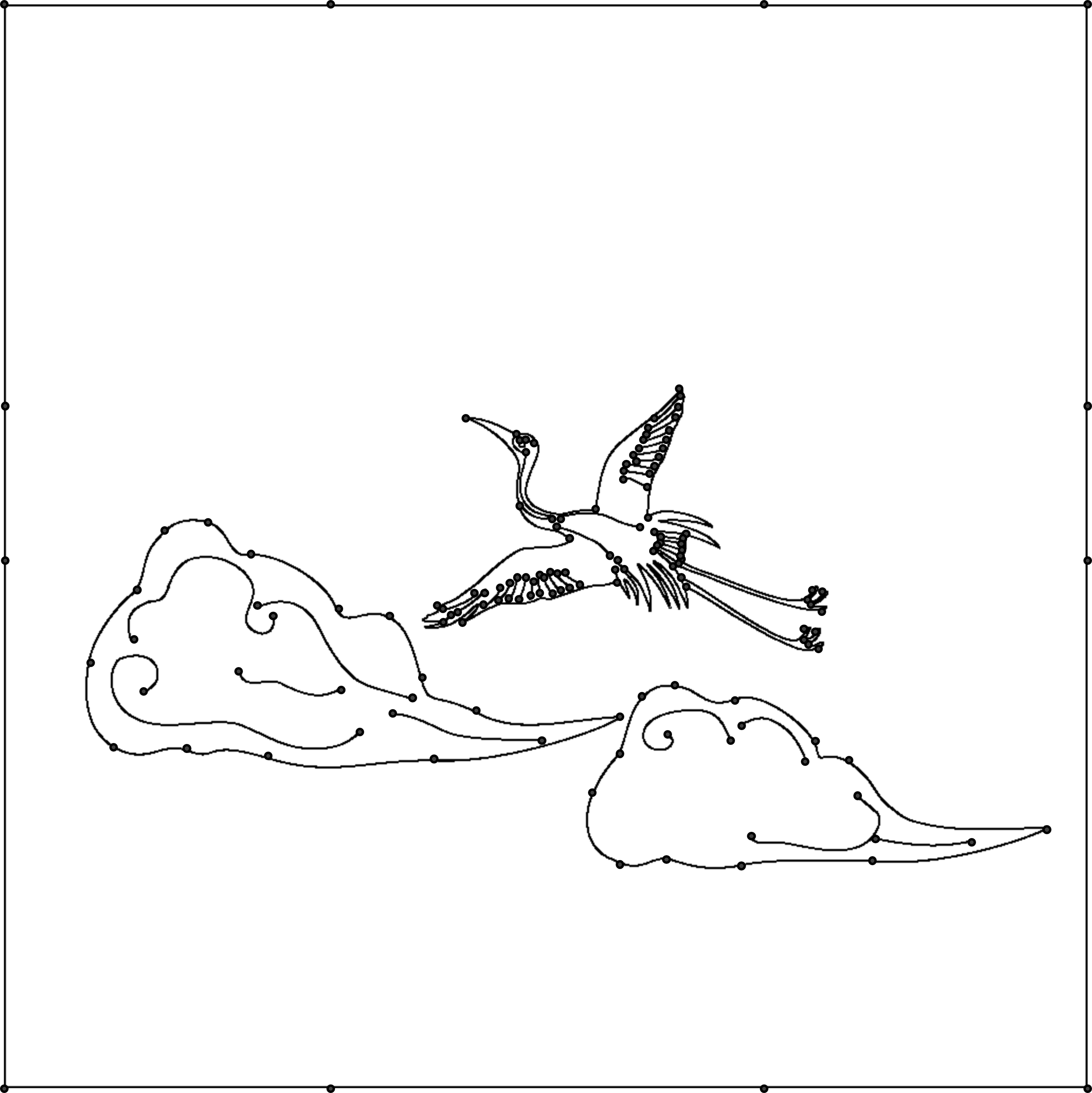
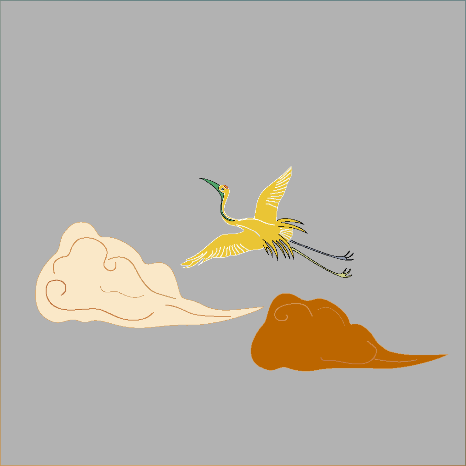
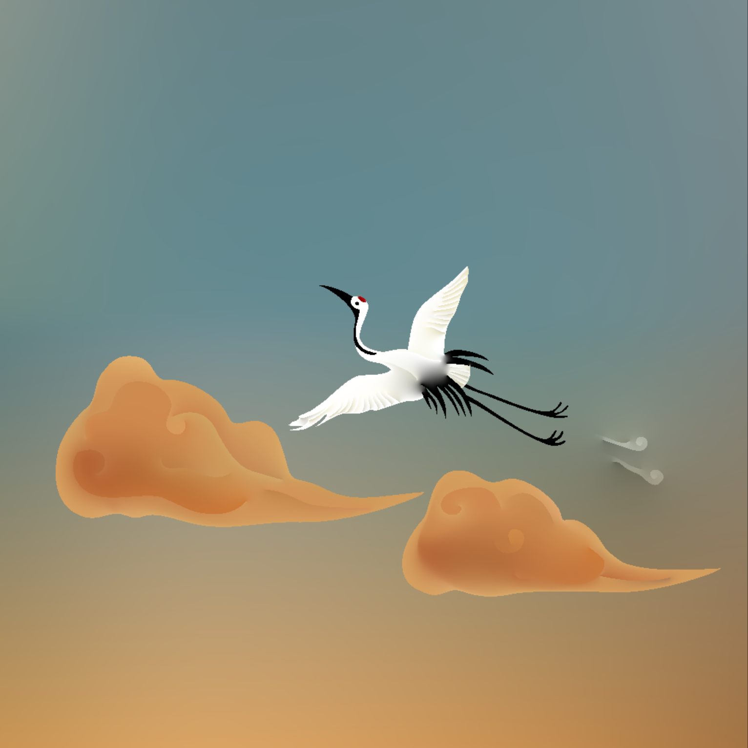
(a) input meshes

(b) input curves

(c) undirected edge graph

(d) unified patch representation

(e) final synthesized image

Figure 1: In this paper, we present an algorithm that unifies the image synthesis of smooth vector graphics containing, gradient meshes, diffusion curves, and Poisson curves in the same scene. Given a set of gradient meshes (a) and diffusion and Poisson curves (b), we first resolve the geometric intersections by forming an undirected edge graph (c), from which a unified patch representation is constructed that divides the domain into separate regions with well-defined Dirichlet and/or Neumann boundary conditions (d). Lastly, the image can be computed with an off-the-shelf Poisson solver (e).

1 Introduction

The field of smooth vector graphics describes image content based on geometric primitives, such as curves or meshes. This is in contrast to raster graphics, which store the color of each pixel explicitly. Smooth vector graphics are a popular tool for the modeling of scale-independent content, such as icons, schematic illustrations, or web content (Hsiao et al., 2023), since images can be synthesized on any output resolution. Basic vector graphics primitives are standardized in the SVG format, which includes the most basic shapes and color gradients. In research, two conceptually different approaches have been developed to extend the artistic control in smoothly-shaded regions. On the one hand, there are gradient meshes (Sun et al., 2007; Lai et al., 2009), which interpolate colors from tensor product surfaces efficiently. And on the other hand, there are curve-based approaches such as diffusion curves (Orzan et al., 2008; Jeschke, 2016) and Poisson curves (Hou et al., 2018) that model the final image as solution to a diffusion problem from user-defined boundary conditions, e.g., curve colors. Both approaches remained incompatible, and research on editing, rasterization, and vectorization, has continued separately on the two research threads (Tian and Günther, 2023). With this paper, we propose a mathematical formulation that allows combining gradient meshes and curve-based approaches consistently for the first time. Fig. 1 gives an example, where gradient meshes are combined with diffusion curves and Poisson curves. To maximize the compatibility with existing methods we take a set of gradient meshes, diffusion curves, and Poisson curves as input, which are well-known primitives that the user interacts with on the front-end. To unify the modeling, we convert those representations first into an intermediate patch representation that specifies for each patch a target Laplacian function and boundary conditions. This intermediate representation is not visible on the user interface and is only used internally to assemble the Poisson problems. We propose to model the pixel color within gradient meshes as solution to a partial differential equation (PDE) in order to match their mathematical treatment with that of curve-based methods. In the conversion process to our patch representation, geometric intersections of gradient meshes and curves get resolved automatically to yield a non-overlapping domain decomposition. In our new formulation, additional types of boundary conditions are added to the existing primitives, which extends the artistic freedom. For example, Neumann conditions can be specified on diffusion curves, as in Bang et al. (2023). To synthesize a raster image for a given output resolution, we rasterize boundary conditions and Laplacians for the respective patches and compute the final image as solution to a Poisson problem. We evaluate the method on various test scenes containing gradient meshes and curve-based primitives. In summary, our contributions are:

• We propose a unified mathematical formulation of gradient meshes and curve-based methods as a Poisson problem.

• We unify the treatment of boundary conditions, which adds (optional) degrees of freedom for artistic control.

• We introduce an automatic conversion algorithm that divides the input primitives into non-overlapping patches.

• We describe a rasterization algorithm for the novel patch formulation that synthesizes images for a given resolution.

For the first time, our approach enables the unified mathematical treatment of gradient meshes and curve-based methods, which have been developed independently for over a decade. Since we take existing gradient mesh and curve formulations as input, our approach achieves high compatibility with existing content creation pipelines. Further, the final algorithm leads to a standard Poisson problem, for which highly optimized numerical solvers readily exist. The benefits of combining gradient meshes and curve-based formulations in the same scene are shown in Fig. 2. While curve-based approaches are useful to create intricate details, it is easier to create larger color gradients with mesh-based approaches (Tian and Günther, 2023). By combining both methods, we are able to generate expressive results that are difficult to obtain with either representation on its own.

In the following section, we first introduce into the necessary background on curve modeling before covering related work on gradient meshes and curve-based formulations. Afterwards, we introduce our unified mathematical description, which is followed by our introduction of the automatic conversion algorithm from standard primitives into our patch formulation. Then, we describe the image synthesis process, user interactions, and lastly we evaluate the approach on numerous scenes, containing both gradient meshes and curve representations.

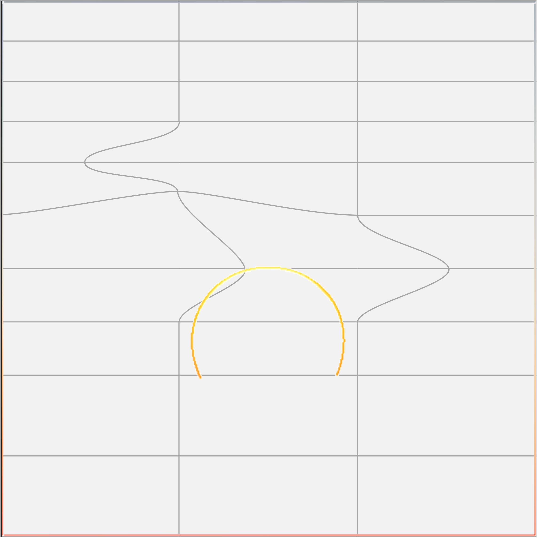
(a) Input primitives

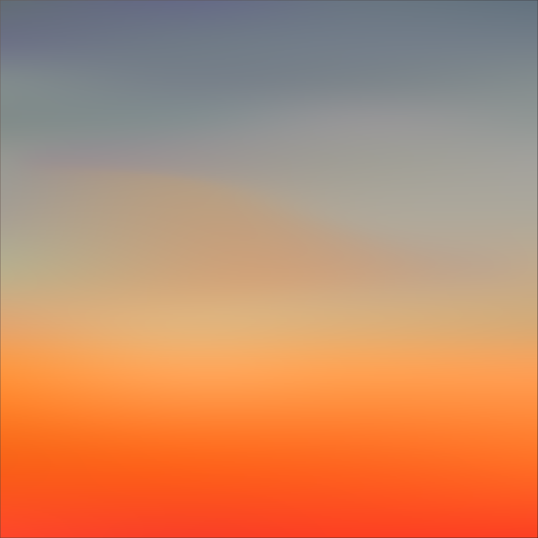
(b) Mesh-based only

(c) Curve-based only

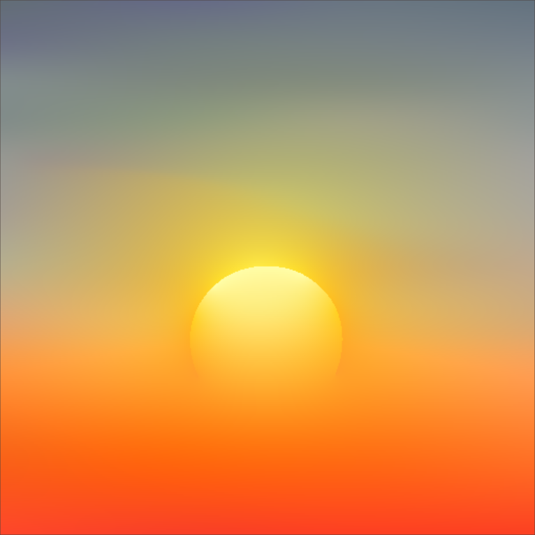
(4) Patches (ours)

Figure 2: This figure shows the benefits of combining gradient meshes with diffusion curves. Gradient meshes are useful for controlling large multi-hue color gradients (the sky), while curve-based methods can add details (the Sun). From left to right, we show the input primitives (gradient meshes and diffusion curves) (a), the result of only rasterizing the gradient meshes (b), the result of only diffusing diffusion curves (c), and lastly our combined representation that contains both (d). Note that the sun diffuses into the sky, mimicking scattering.

2 Background

In this section, we formally introduce the notation used to describe mesh-based and curve-based vector graphics primitives. For a detailed coverage, we refer to a recent survey (Tian and Günther, 2023).

2.1 Bézier Curves

In this paper, we denote Bézier curves of degree $n$ as parametric curves $\gamma(t):[0,1]\rightarrow\mathbb{R}^{m}$ in $m$-dimensional space:

$$\gamma(t)=\sum_{i=0}^{n}B_{i}^{n}(t)\cdot\mathbf{b}_{i}\;\;\textrm{with}\;\;B_{i}^{n}(t)=\binom{n}{i}t^{i}(1-t)^{n-i},$$ (1)

where $B_{i}^{n}(t)$ are the Bernstein basis functions, and $\mathbf{b}_{i}\in\mathbb{R}^{m}$ are the Bézier control points. The curve tangent is denoted by $\dot{\gamma}(t)=\frac{\mathrm{d}\gamma(t)}{\mathrm{d}t}$. A cubic Bézier curve ($n=3$) in a two-dimensional plane ($m=2$) has four control points $\mathbf{b}_{0}$, $\mathbf{b}_{1}$, $\mathbf{b}_{2}$, and $\mathbf{b}_{3}$, and has by convention a right-oriented curve normal $\gamma_{n}(t):[0,1]\rightarrow\mathbb{R}^{2}$:

$$\gamma_{n}(t)=\begin{pmatrix}0&1\\ -1&0\end{pmatrix}\frac{\dot{\gamma}(t)}{\|\dot{\gamma}(t)\|}.$$ (2)

Thus, given the control points $\mathbf{b}_{0}$, $\mathbf{b}_{1}$, $\mathbf{b}_{2}$, $\mathbf{b}_{3}$, the curve point $\gamma(t)$, tangent $\dot{\gamma}(t)$, and normal $\gamma_{n}(t)$ can be evaluated for each $t$. Multiple Bézier curves can be concatenated with suitable continuity conditions to assemble a Bézier-spline curve (Farin, 2002).

2.2 Mesh-based Methods

Mesh-based vector graphics primitives specify color gradients inside connected regions by using interpolation. Depending on the mesh topology, they are categorized into triangular, rectangular, and irregular meshes. Our work focuses on rectangular meshes.

Rectangular Mesh

By generalization of the Bézier curves in Eq. (1), a Bézier tensor-product surface $f(u,v):[0,1]^{2}\rightarrow\mathbb{R}^{m}$ is

$$f(u,v)=\sum_{i=0}^{n_{1}}\sum_{j=0}^{n_{2}}B_{i}^{n_{1}}(u)\cdot B_{j}^{n_{2}}(v)\cdot f_{i,j}.$$ (3)

Later, we use the symbol $\partial_{u}f_{i,j}:=\frac{\partial f(u,v)}{\partial u}_{|u=u_{i},v=v_{j}}$ to abbreviate the evaluation of a derivative at a discrete location. Each tensor-product surface is bound by four Bézier curves $f(u,0)$, $f(u,1)$, $f(0,v)$ and $f(1,v)$ with $u,v\in[0,1]$.

Price and Barrett (2006) used bi-cubic surfaces, which have a degree of $n_{1}=n_{2}=3$. The direct editing of its 16 control points $f_{0,0},\dots,f_{3,3}$ is cumbersome. Fortunately, a bi-cubic tensor-product surface can be expressed as a Ferguson patch, cf. Sun et al. (2007):

$$f(u,v)=\mathbf{t}(u)^{\mathrm{T}}\cdot\mathbf{C}^{\mathrm{T}}\cdot\mathbf{Q}\cdot\mathbf{C}\cdot\mathbf{t}(v)$$ (4)

with the monomial basis $\mathbf{t}(t)=(1,t,t^{2},t^{3})^{\mathrm{T}}$ and the matrices:

$$\mathbf{C}=\begin{pmatrix}1&0&-3&2\\ 0&0&3&-2\\ 0&1&-2&1\\ 0&0&-1&1\end{pmatrix},\mathbf{Q}=\begin{pmatrix}f_{0,0}&f_{0,3}&\partial_{v}f_{0,0}&\partial_{v}f_{0,3}\\ f_{3,0}&f_{3,3}&\partial_{v}f_{3,0}&\partial_{v}f_{3,3}\\ \partial_{u}f_{0,0}&\partial_{u}f_{0,3}&\partial_{u}\partial_{v}f_{0,0}&\partial_{u}\partial_{v}f_{0,3}\\ \partial_{u}f_{3,0}&\partial_{u}f_{3,3}&\partial_{u}\partial_{v}f_{3,0}&\partial_{u}\partial_{v}f_{3,3}\end{pmatrix}$$

To simplify the modeling, the mixed partial derivatives are commonly set to zero, i.e., $\partial_{u}\partial_{v}f_{i,j}=0$, and thus, a function $f(u,v)$ can be controlled by the user by specifying the values $f_{i,j}$ and the tangent handles $\partial_{u}f_{i,j}$ and $\partial_{v}f_{i,j}$ at the four corners $i,j\in\{0,3\}$, see Fig. 3a. A gradient mesh consists of multiple Ferguson patches that are stitched together with suitable continuity condition. The functions $f(u,v)$ that are modeled by the gradient mesh are the position $\mathbf{x}(u,v)$ and the color $\mathbf{c}(u,v)$. Thus, the degrees of freedom are $\mathbf{x}_{i,j}$, $\mathbf{c}_{i,j}$ and the tangent handles $\partial_{u}\mathbf{x}_{i,j}$, $\partial_{u}\mathbf{c}_{i,j}$ and $\partial_{v}\mathbf{x}_{i,j}$, $\partial_{v}\mathbf{c}_{i,j}$ at the four corners $(i,j)\in\{(0,0),(0,3),(3,0),(3,3)\}$. To model holes in surfaces, Lai et al. (2009) proposed to split gradient meshes along discontinuities. Barendrecht et al. (2018) enabled local refinement of cubic rectangular patches. In line with many other papers (Xiao et al., 2012, 2015; Wan et al., 2018; Wei et al., 2019), we likewise base our description of gradient meshes on Sun et al. (2007), see Eq. (4).

Triangular and Irregular Meshes

As an alternative to rectangular meshes, triangle-based patches have been explored, where the patch boundaries are curved edges (Xia et al., 2009; Xiao et al., 2022). Control over the continuity across adjacent patches is desirable (Liao et al., 2012; Zhou et al., 2014). To this end, quadratic triangle configuration B-splines (TCBs) (Cao et al., 2019; Schmitt, 2019) have been used by Zhu et al. (2022) to model color variations while staying $C^{1}$ continuous. An example for irregular patches are the polygonal patches of Swaminarayan and Prasad (2006), who used constant colors in the interior. With the introduction of Bézigons (Yang et al., 2015) closed regions have been bounded by Bézier curves. For color interpolation in the interior, several options are available (Hettinga et al., 2019), including cubic mean value coordinates (Li et al., 2013). Since the methods above use differentiable interpolants, they are compatible with our approach.

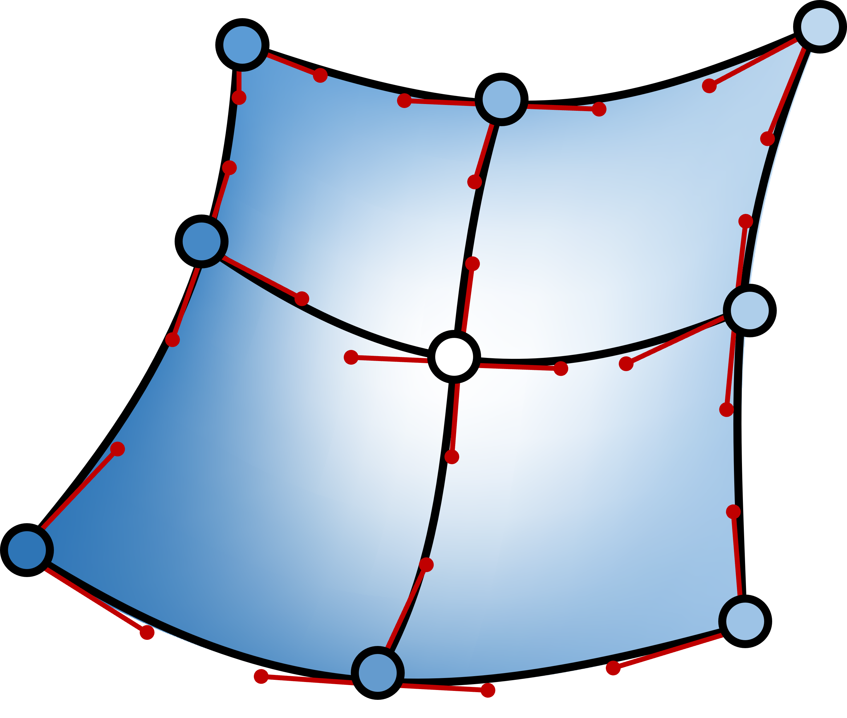
(a) Gradient Mesh

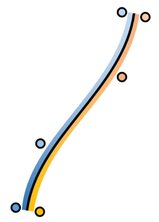
(b) Diffusion Curve

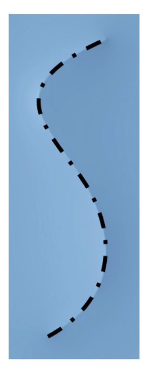
(c) Poisson Curve

Figure 3: Overview of the three mesh and curve primitives that are used in our framework. Gradient meshes (a) are assembled from Ferguson patches, which contain smooth color gradients and are controlled by colors at the corners and tangent handles. Diffusion curves (b) define a color on the left and right side, typically by piecewise linear interpolation among color stops. Poisson curves (c) allow for the modeling of cusps and highlights by locally adjusting the Laplacian of the underlying color field.

2.3 Curve-based Methods

With curve-based methods, color gradients are the result of a diffusion process from colors given at the domain boundaries.

Diffusion Curves

Originally, diffusion curves (Orzan et al., 2008) are Bézier curves $\gamma(t)$ with a piecewise linear color on the left and right side, i.e., $\mathbf{c}_{l}(t)$ and $\mathbf{c}_{r}(t)$. The colors serve as Dirichlet boundary conditions in a diffusion process that produces smooth color gradients, see Fig. 3b. The reformulation of Jeschke et al. (2009) treats diffusion curves as domain boundaries $\partial\Omega$ of a smoothly shaded region $\Omega$. The color field of the shaded region $\mathbf{c}(\mathbf{x})$ is as smooth as possible and meets the boundary color $\mathbf{g}(\mathbf{x})$, as specified by the colors on the left and right hand side of the diffusion curve.

$$\mathbf{c}(\mathbf{x})=\begin{cases}\Delta\mathbf{c}(\mathbf{x})=0,&\mathbf{x}\in\Omega\backslash\partial\Omega\\ \hphantom{\Delta}\mathbf{c}(\mathbf{x})=\mathbf{g}(\mathbf{x}),&\mathbf{x}\in\partial\Omega\end{cases}$$ (5)

Follow-up research on rendering (Pang et al., 2011; Sun et al., 2014; Bang et al., 2023), vectorization (Zhao et al., 2017; Lu et al., 2019) and editing (Jeschke et al., 2011; Lu et al., 2020) utilized this formulation. To provide more control over the color gradients, Bezerra et al. (2010) controlled the strength and direction of the diffusion. Alternatively, Sun et al. (2012) introduced textures in diffusion curves. Several renderers have been proposed by now that are able to rasterize diffusion curves, including ray tracing approaches (Bowers et al., 2011; Prévost et al., 2015), Monte Carlo methods (Sawhney and Crane, 2020; Sawhney et al., 2023; Sugimoto et al., 2023), and boundary element methods (Ilbery et al., 2013; Bang et al., 2023; Chen et al., 2024).

Poisson Curves

By introducing Poisson vector graphics, Hou et al. (2018) edited the gradient in the domain by introducing a desired (piecewise-constant) Laplacian $\mathbf{f}(\mathbf{x})$:

$$\mathbf{c}(\mathbf{x})=\begin{cases}\Delta\mathbf{c}(\mathbf{x})=\mathbf{f}(\mathbf{x}),&\mathbf{x}\in\Omega\backslash\partial\Omega\\ \hphantom{\Delta}\mathbf{c}(\mathbf{x})=\mathbf{g}(\mathbf{x}),&\mathbf{x}\in\partial\Omega\end{cases}$$ (6)

Thus, rather than looking for the smoothest possible color gradient (via $\mathbf{f}(\mathbf{x})=0$), bumps and discontinuities can be introduced in the color gradient, which is locally controlled by the user by drawing curve and region primitives, see Fig. 3c. Non-constant Laplacians in Poisson regions have been described by raster images, and were utilized for color transfer between images (Fu et al., 2019) and for image vectorization (Fu et al., 2024). Alternatively, Finch et al. (2011) proposed to constrain high-order derivatives, seeking solutions that are harmonic in their Laplacian domain, i.e., $\Delta^{2}\mathbf{c}(\mathbf{x})=\mathbf{0}$. With this formulation, extrapolation may create new extrema at unconstrained positions (Finch et al., 2011; Boyé et al., 2012), which requires manual adjustment of control points (Finch et al., 2011) or a non-linear optimization (Jacobson et al., 2012). Further, the diffused color range is tied to the scene geometry, which may lead to oversaturation (Jeschke, 2016) when scaling objects. In our work, we concentrate on the Poisson formulation in Eq. (6), which includes the diffusion curves in Eq. (5) as special case. Poisson vector graphics (Hou et al., 2018) have led to a new line of work on the control over color gradients within smooth vector graphics. In this paper, we seek to utilize the well-established gradient meshes (Sun et al., 2007), which so far have not been incorporated into this framework.

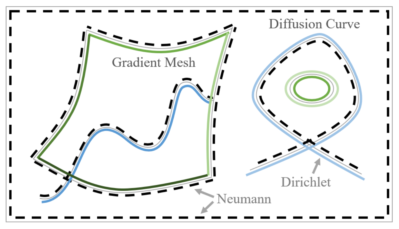
(a) Input Primitives

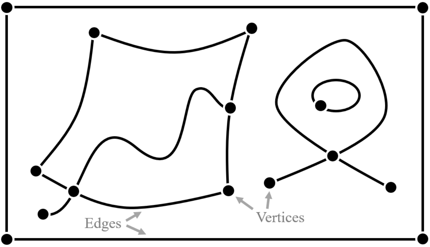
(b) Edge Graph

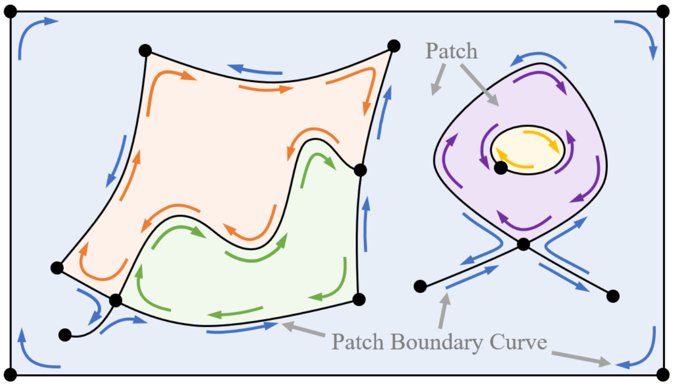
(c) Unified Patches

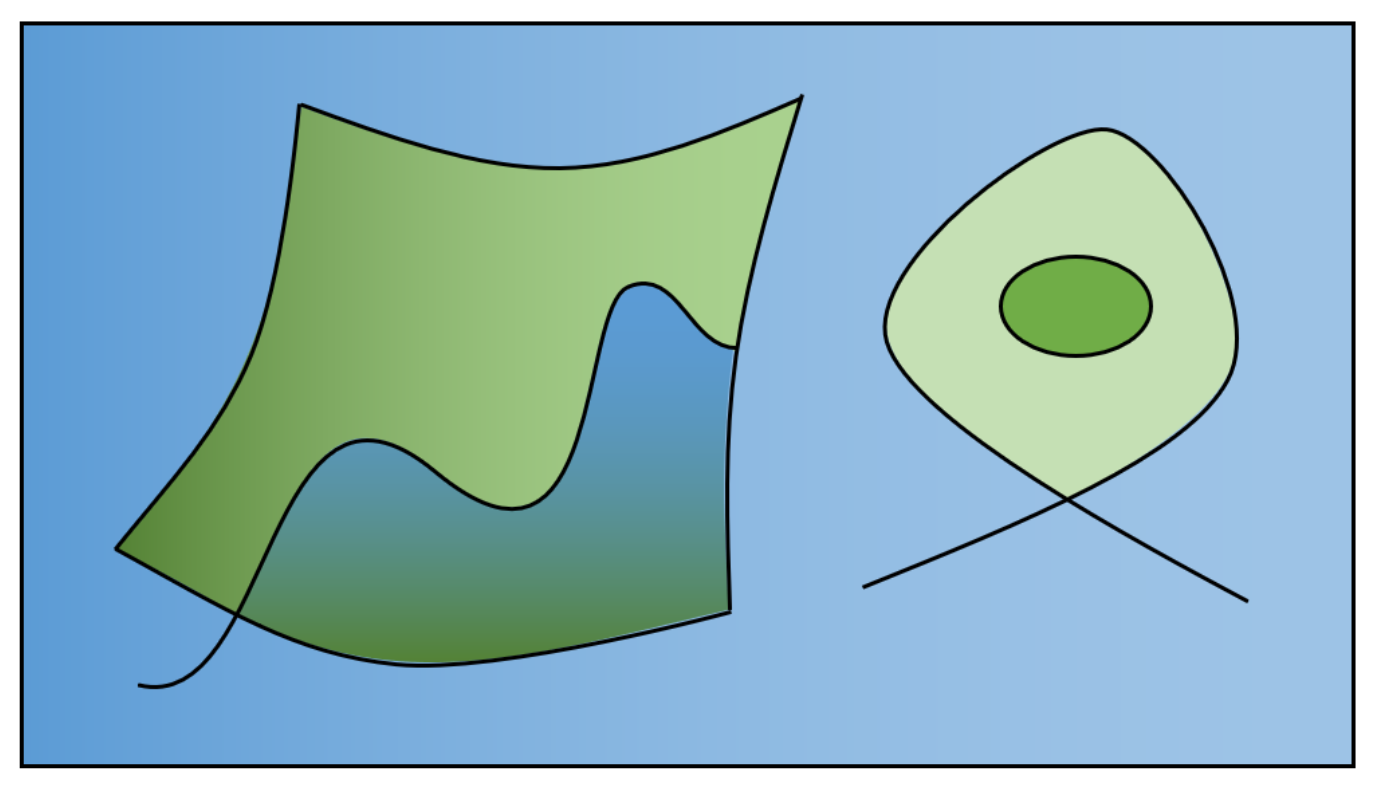
(d) Image Synthesis

Figure 4: Schematic overview of our generalized smooth vector graphics pipeline. (a) Input to our method is a collection of (extended) gradient meshes, (extended) diffusion curves, and Poisson curves. (b) The input primitives are converted and inserted into an edge graph that resolves the intersection of input primitives. (c) From the edge graph a unified patch data structure is formed that defines patches as closed regions with boundary conditions according to the underlying input primitives. (d) The unified patch data structure specifies the ingredients for a Poisson problem that is solved to synthesize the final image.

3 Method Overview

Our goal is to synthesize raster images for vector graphics scenes that contain mesh-based and curve-based primitives at the same time. Usually, mesh-based and curve-based methods are rasterized in fundamentally different ways. While mesh-based approaches use interpolation, curve-based methods solve a Poisson problem. To model both approaches consistently, we describe the mesh-based approaches as solution to a Poisson problem that is identical to interpolation in the absence of any curve-based primitives. A user of our system may decide to draw curve-based primitives that intersect each other or intersect with mesh-based primitives. To formulate the Poisson problem, the scene is decomposed into non-overlapping regions for which boundary conditions are defined and for which a Laplacian is determined that controls the color gradient in the interior. We formulate the rasterization of smooth vector graphics as a pipeline consisting of multiple steps, see Fig. 4.

1. Input Primitives. Input to our method are standard smooth vector graphics primitives, such as gradient meshes, diffusion curves, and Poisson curves, which are created and edited by the user. We extend gradient meshes and diffusion curves by allowing the user to specify Dirichlet conditions and homogeneous Neumann conditions on either side.

2. Edge Graph. Both the extended gradient meshes and the extended diffusion curves are inserted into an undirected edge graph data structure (Gangnet et al., 1989), which records and resolves all intersections of boundary curves.

3. Unified Patches. By traversing the edge graph, we define closed, non-overlapping regions that have consistent boundary conditions. The interior of each patch is equipped with a Laplacian function that is either homogeneous, or sampled from a gradient mesh and/or multiple Poisson curves.

4. Image Synthesis. Given the patches with their boundary conditions, we solve the Poisson problem for each patch independently with an off-the-shelf Poisson solver.

In the following, the four steps are explained in more detail.

4 Input Primitives

Input to our approach is a collection of extended gradient meshes $\mathcal{G}$, a collection of extended diffusion curves $\mathcal{D}$ and a collection of Poisson curves $\mathcal{P}$. Those three types of input primitives are drawn by the user and can be edited and controlled by manipulation of control points, tangent handles, and color stops, identical to the editing processes of conventional diffusion curves, gradient meshes, and Poisson curves (Tian and Günther, 2023). In the following, we explain how the primitives are defined and how they are extended in our framework.

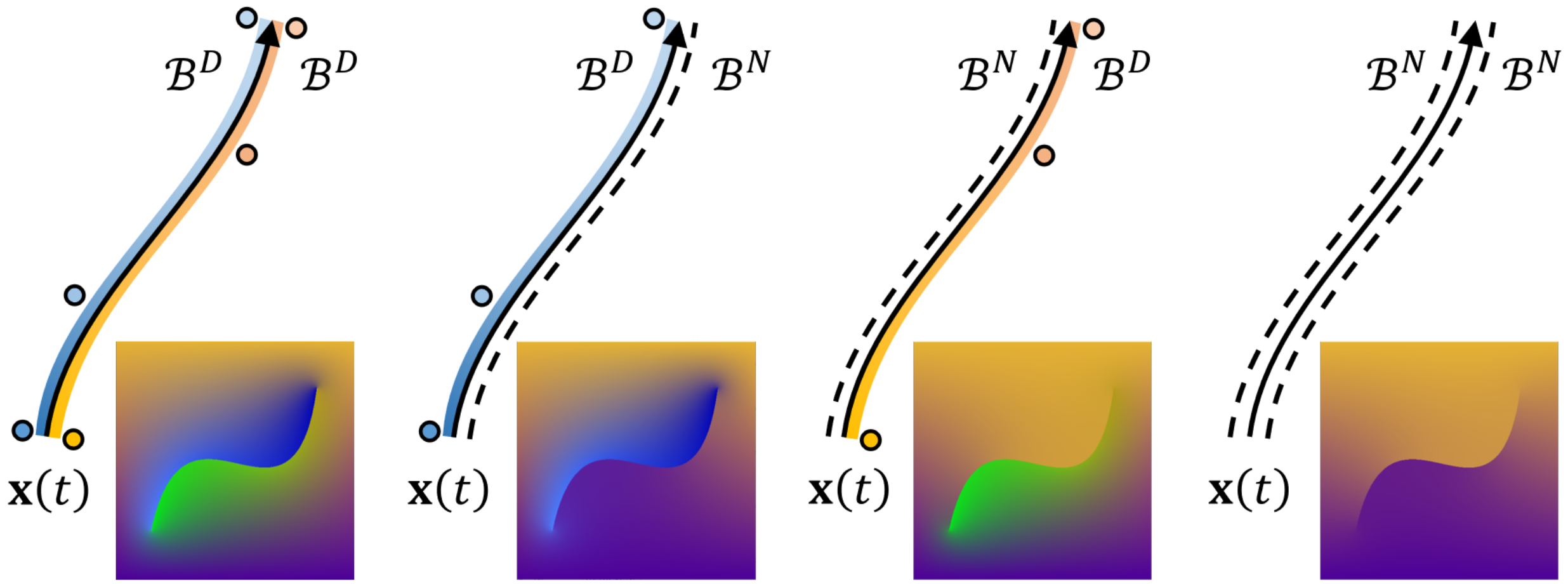
Figure 5: Input boundary curves consist of a spatial curve $\mathbf{x}(t)$ and boundary conditions on the left and right side, which may either be a Dirichlet boundary condition $\mathcal{B}^{D}$ (shown as colored line with control points) or a homogeneous Neumann boundary condition $\mathcal{B}^{N}$ (shown as a dashed line).

4.1 Definition

First, we introduce an input boundary curve, which is a triplet $(\mathbf{x}(t),\mathcal{B}_{l},\mathcal{B}_{r})$, as shown in Fig. 5. It consists of:

• the spatial curve $\mathbf{x}(t)$,

• a left boundary condition $\mathcal{B}_{l}$,

• and a right boundary condition $\mathcal{B}_{r}$.

The spatial location of the input boundary curve is given by a cubic Bézier spline $\mathbf{x}(t):\mathbb{R}\rightarrow\mathcal{U}$, where $\mathcal{U}\subset\mathbb{R}^{2}$ denotes the image domain. The curve parameter range $t\in[t_{0},t_{1}]$ defines the orientation of the curve. We require $t_{0}<t_{1}$, where the curve begins at $t_{0}$ and ends at $t_{1}$. This gives rise to the notion of a left side and a right side of the curve. Each input boundary curve will later define a boundary condition in the field $\mathbf{c}(\mathbf{x}):\mathcal{U}\rightarrow\mathcal{C}$, where $\mathcal{C}\subset\mathbb{R}^{3}$ is the color space. The boundary condition is either a Dirichlet boundary condition $\mathcal{B}^{D}$ with color $\mathbf{c}(t)$ or a homogeneous Neumann boundary condition $\mathcal{B}^{N}$ with boundary normal $\mathbf{x}_{n}(t)$, cf. Eq. (2):

$$\mathcal{B}^{D} =\begin{cases}\mathbf{c}(\mathbf{x})_{|\mathbf{x}=\mathbf{x}(t)}=\mathbf{c}(t)&\,\qquad\textrm{Dirichlet with $\mathbf{c}(t)$}\end{cases}$$ (7)

$$\mathcal{B}^{N} =\begin{cases}\frac{\partial\mathbf{c}(\mathbf{x})}{\partial\mathbf{x}}_{|\mathbf{x}=\mathbf{x}(t)}\cdot\mathbf{x}_{n}(t)=0&\textrm{homogen. Neumann}\end{cases}$$ (8)

For notational convenience, we name the left boundary condition $\mathcal{B}_{l}\in\{\mathcal{B}^{D},\mathcal{B}^{N}\}$ and the right boundary condition $\mathcal{B}_{r}\in\{\mathcal{B}^{D},\mathcal{B}^{N}\}$. Adding inhomogeneous Neumann conditions would be a straightforward extension that would, however, add further complexity to the user interface.

Extended Gradient Mesh

A gradient mesh that consists of a single Ferguson patch as in Eq. (4), with position $\mathbf{x}(u,v)$ and color $\mathbf{c}(u,v)$, gives rise to four clock-wise oriented boundary curves with positions $\mathbf{x}(t)\in\{\mathbf{x}(1,1-t),\mathbf{x}(1-t,0),\mathbf{x}(0,t),\mathbf{x}(t,1)\}$. Using the clock-wise orientation of the boundary curves, we set the right boundary conditions (i.e., the inside of the gradient mesh) to a Dirichlet condition $\mathcal{B}_{r}=\mathcal{B}^{D}$ by using the corresponding colors $\mathbf{c}(t)\in\{\mathbf{c}(1,1-t),\mathbf{c}(1-t,0),\mathbf{c}(0,t),\mathbf{c}(t,1)\}$. Our extension compared to a regular gradient mesh is that we add the definition of a boundary condition on the outside of the gradient mesh, as well. The left boundary condition (i.e., the outside of the gradient mesh) is by default set to a homogeneous Neumann condition $\mathcal{B}_{l}=\mathcal{B}^{N}$. The user may change this to a Dirichlet condition if desired. For a gradient mesh that consists of multiple connected Ferguson patches, input boundary curves are only generated for the outermost Ferguson patch boundaries, which coincide with the boundary of the gradient mesh. Adding the interior Ferguson patch boundaries is neither necessary nor useful, since the smooth color gradient in the interior of the gradient mesh will be fully defined by the Laplacian of its Ferguson patches. Fig. 6 demonstrates this at the example of a closed diffusion curve (circle), which intersects a gradient mesh (blue). If interior patch boundaries were added, it would introduce unwanted diffusion barriers that are counter-intuitive.

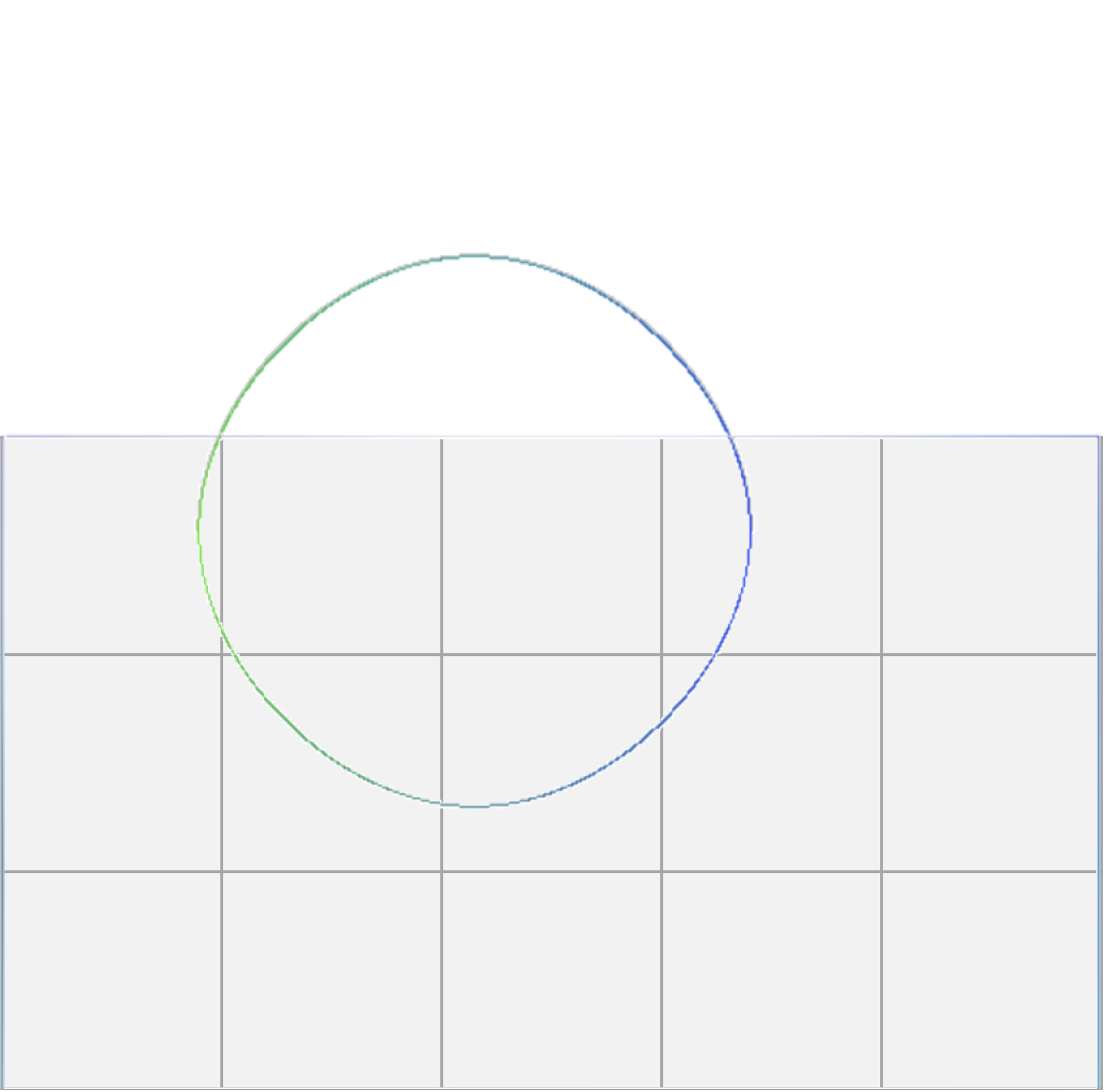
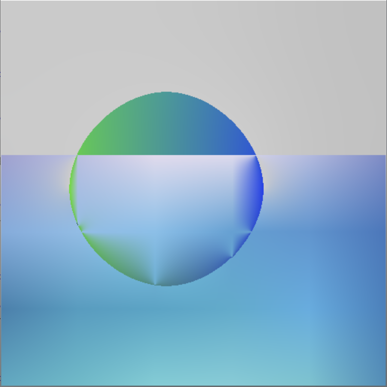
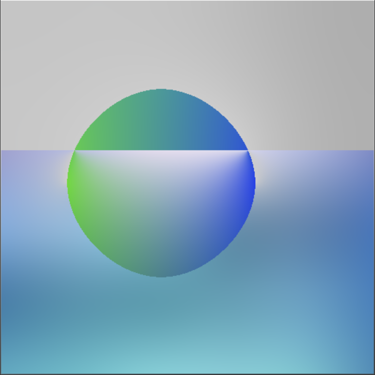
input primitives

w/ inner boundaries

w/o inner boundaries

Figure 6: When constructing input boundary curves, the inner edges of gradient meshes are not added, since they would create diffusion barriers. The inner edges are not needed, since the color gradients are fully determined by the gradient mesh Laplacian, which is considered in the Poisson problem.

Extended Diffusion Curve

A diffusion curve $\gamma(t):\mathbb{R}\rightarrow\mathcal{U}$ with left color $\mathbf{c}_{l}(t):\mathbb{R}\rightarrow\mathcal{C}$ and right color $\mathbf{c}_{r}(t):\mathbb{R}\rightarrow\mathcal{C}$ translates to an input boundary curve by setting $\mathbf{x}(t)=\gamma(t)$ and by applying Dirichlet conditions on the left and right with $\mathcal{B}_{l}=\mathcal{B}^{D}$ and $\mathcal{B}_{r}=\mathcal{B}^{D}$. Same as Bang et al. (2023), we extend diffusion curves by allowing to replace the Dirichlet conditions with homogeneous Neumann conditions.

Poisson Curve

Analogous to diffusion curves, we define a Poisson curve as a spatial curve $\mathbf{p}(t):\mathbb{R}\rightarrow\mathcal{U}$ with a target Laplacian function on the left $\mathbf{f}_{l}(t):\mathbb{R}\rightarrow\mathbb{R}^{3}$ and on the right $\mathbf{f}_{r}(t):\mathbb{R}\rightarrow\mathbb{R}^{3}$. Upon rasterization, the sides cover the pixels $\mathcal{F}_{l}\subseteq\mathcal{U}$ and $\mathcal{F}_{r}\subseteq\mathcal{U}$, respectively, with $\mathbf{f}_{l}(\mathbf{x}):\mathcal{F}_{l}\rightarrow\mathbb{R}^{3}$ and $\mathbf{f}_{r}(\mathbf{x}):\mathcal{F}_{r}\rightarrow\mathbb{R}^{3}$ being the target Laplacian at spatial coordinates $\mathbf{x}\in\mathcal{D}$. To obtain shading consistency, Hou et al. (2018) required the functions $\mathbf{f}_{l}(t)$ and $\mathbf{f}_{r}(t)$ to sum to zero along the curve, i.e., $\forall\mathbf{x}:\mathbf{f}_{l}(t)=-\mathbf{f}_{r}(t)$. For notational convenience, we collectively refer to a sampling from the left or right side of the target Laplacian as $\mathbf{f}_{\mathbf{p}(t)}(\mathbf{x}):\mathcal{D}\rightarrow\mathbb{R}^{3}$:

$$\mathbf{f}_{\mathbf{p}(t)}(\mathbf{x})=\begin{cases}\mathbf{f}_{l}(\mathbf{x})\cdot\gamma_{l}(\mathbf{x})&\mathbf{x}\in\mathcal{F}_{l}\\ \mathbf{f}_{r}(\mathbf{x})\cdot\gamma_{r}(\mathbf{x})&\mathbf{x}\in\mathcal{F}_{r}\\ \mathbf{0}&\textrm{else}\end{cases}$$ (9)

where $\gamma_{l}(\mathbf{x})$ is the number of adjacent pixels that belong to $\mathcal{F}_{r}$ and $\gamma_{r}(\mathbf{x})$ is the number of adjacent pixels in $\mathcal{F}_{l}$, which are used for normalization, cf. Hou et al. (2018). An overview of the supported target Laplacians $\mathbf{f}_{l}(t)$ is shown in Fig. 7.

 

 

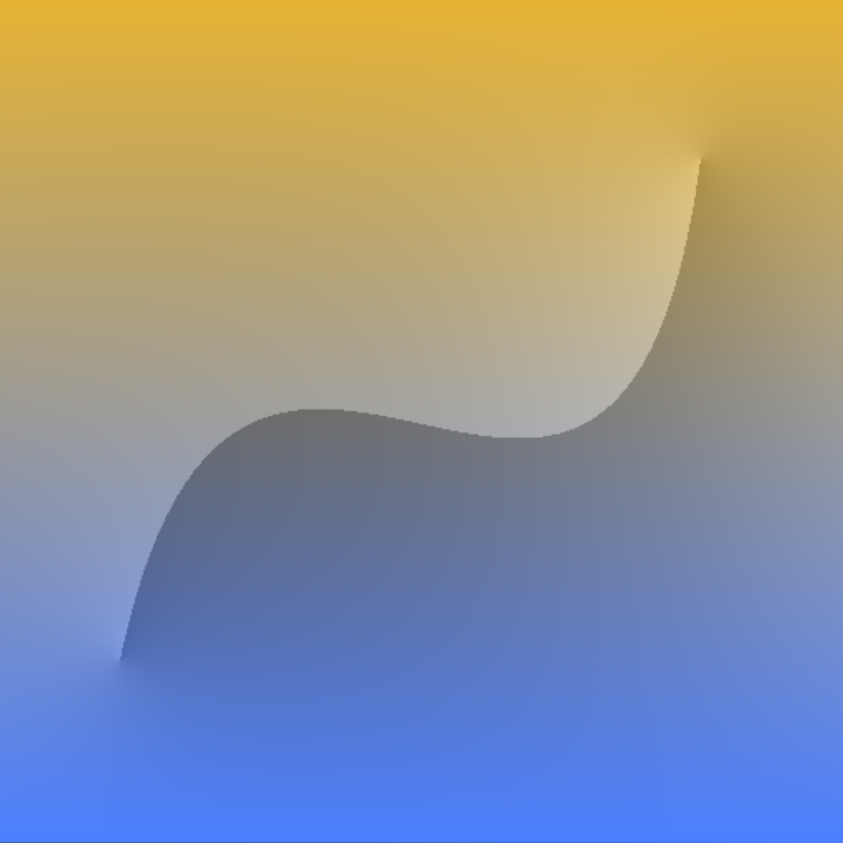
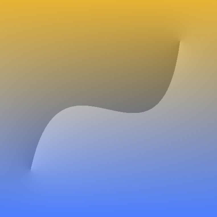
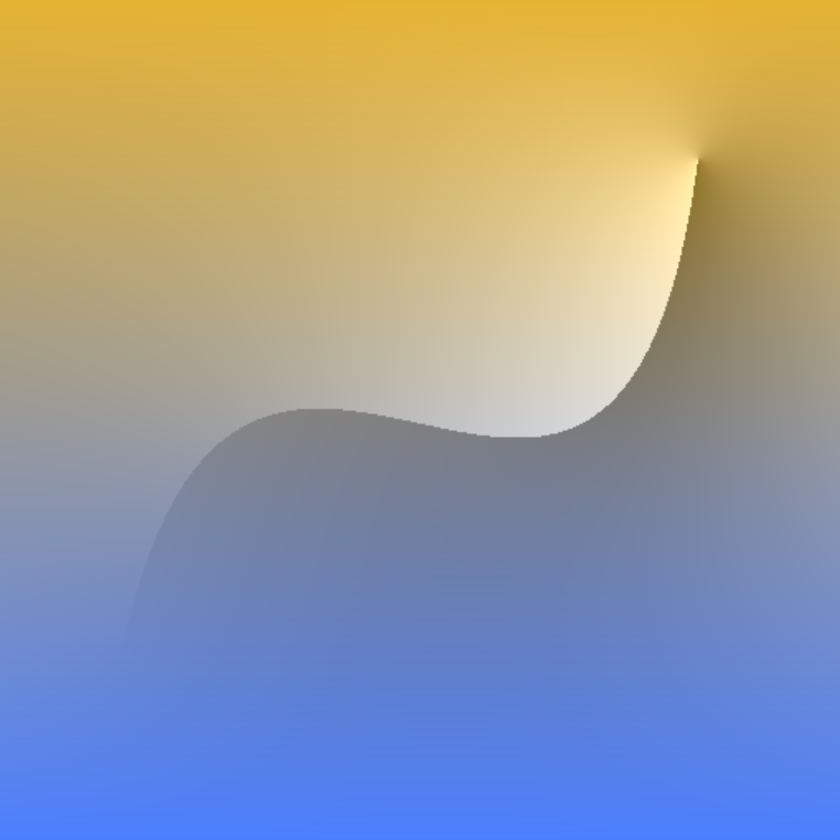
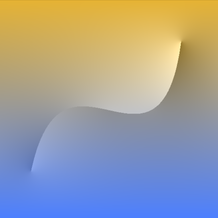
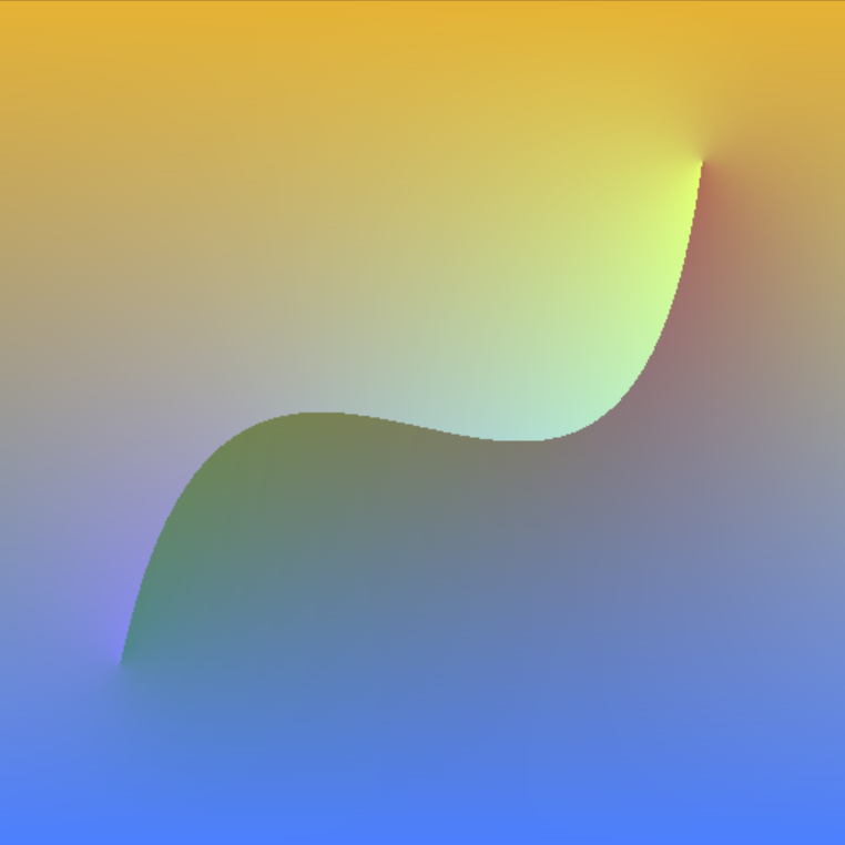
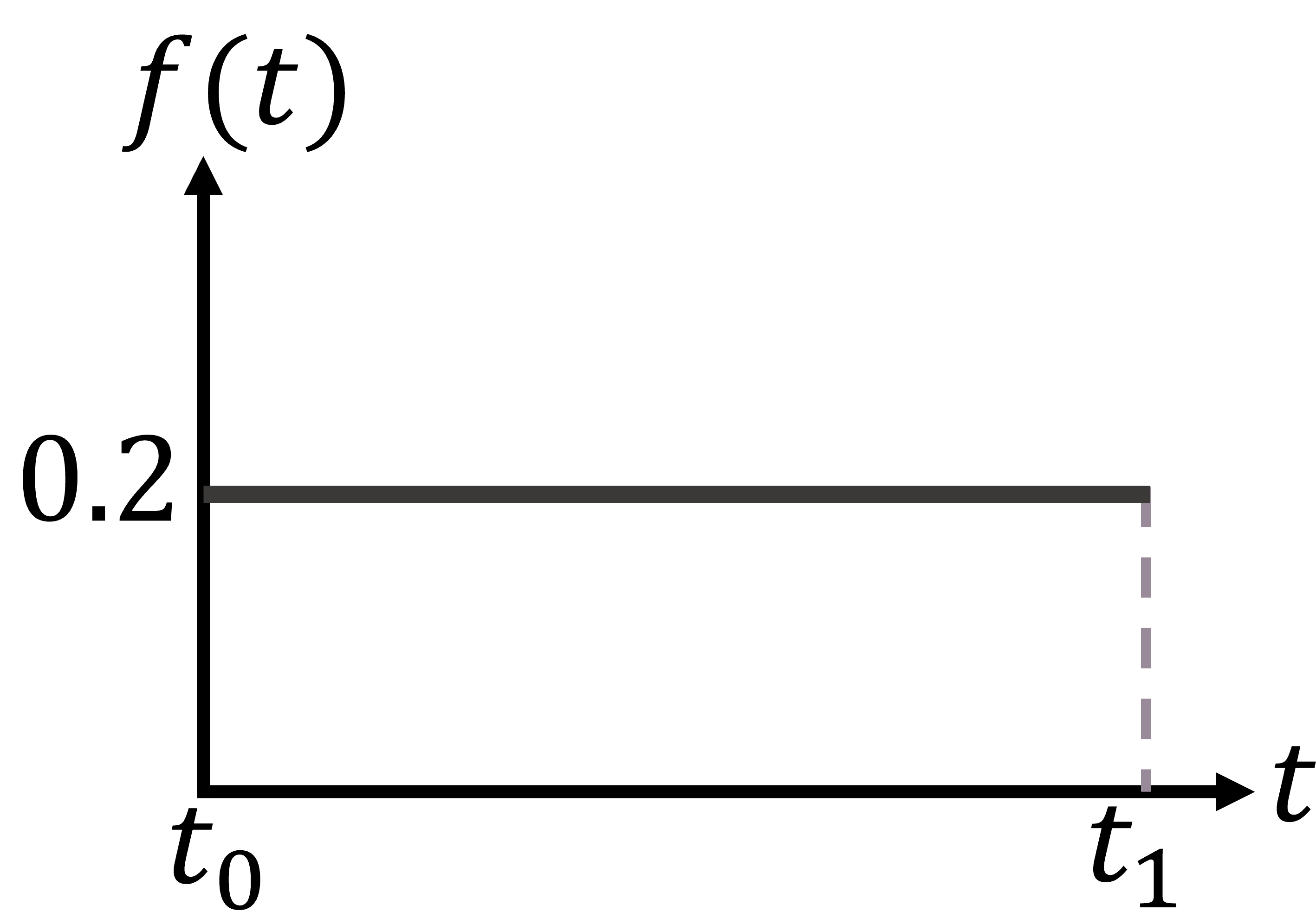
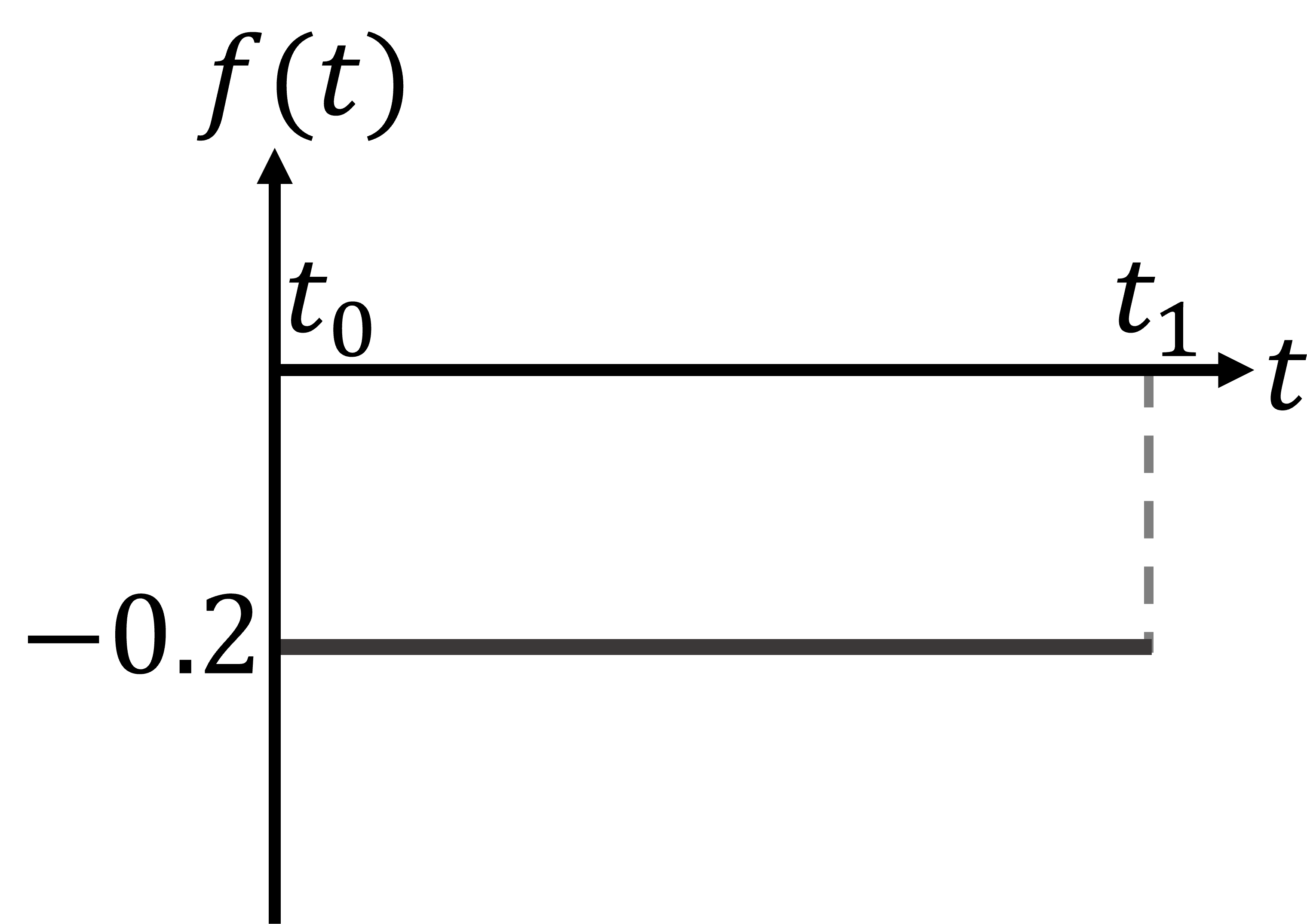
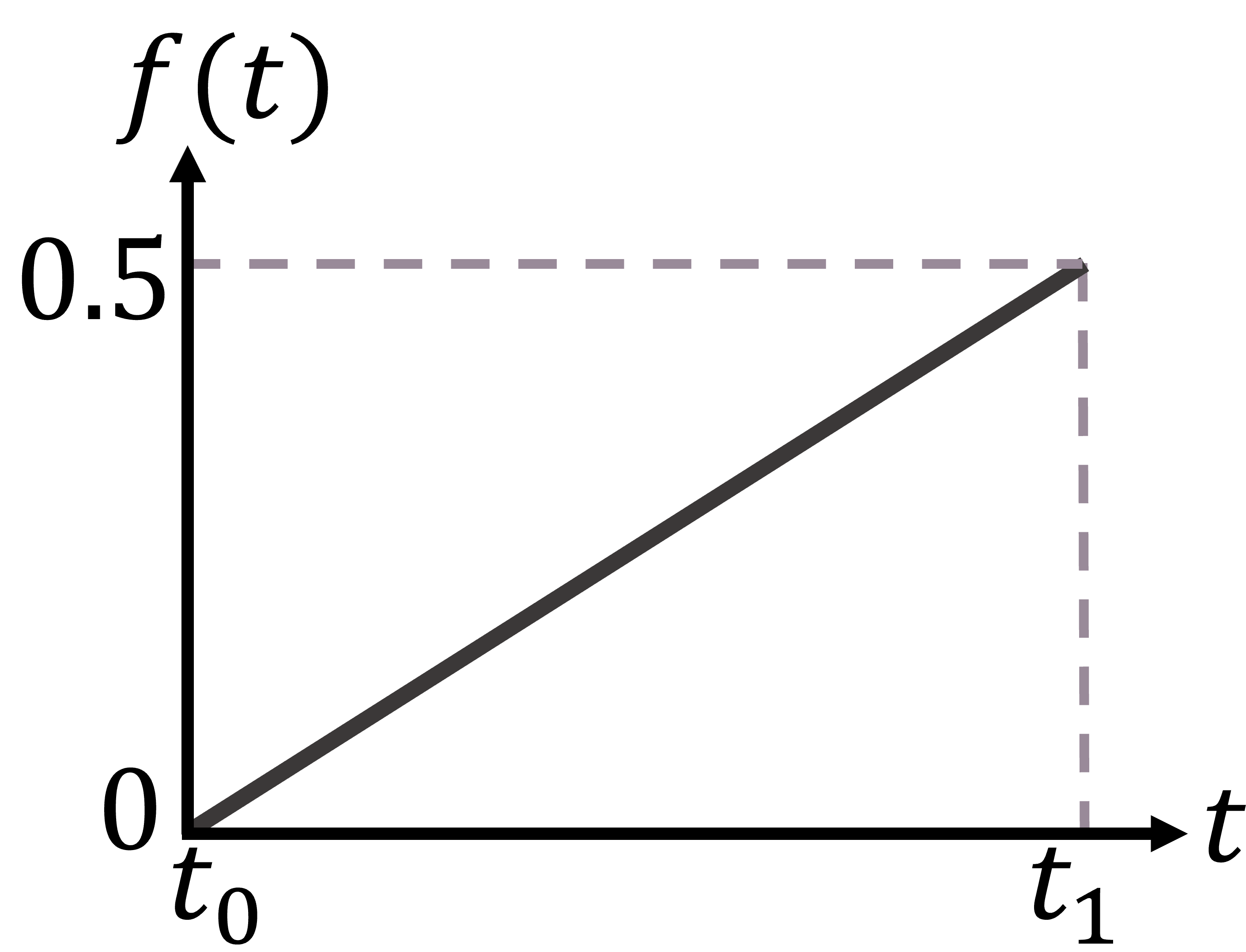
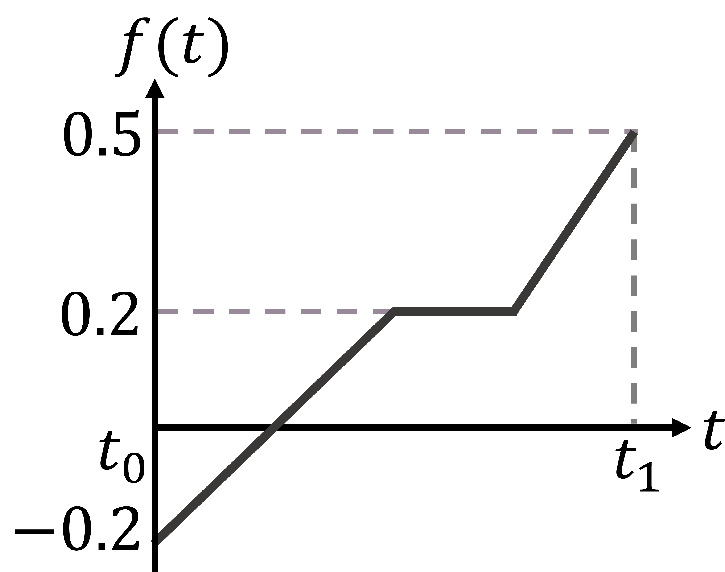
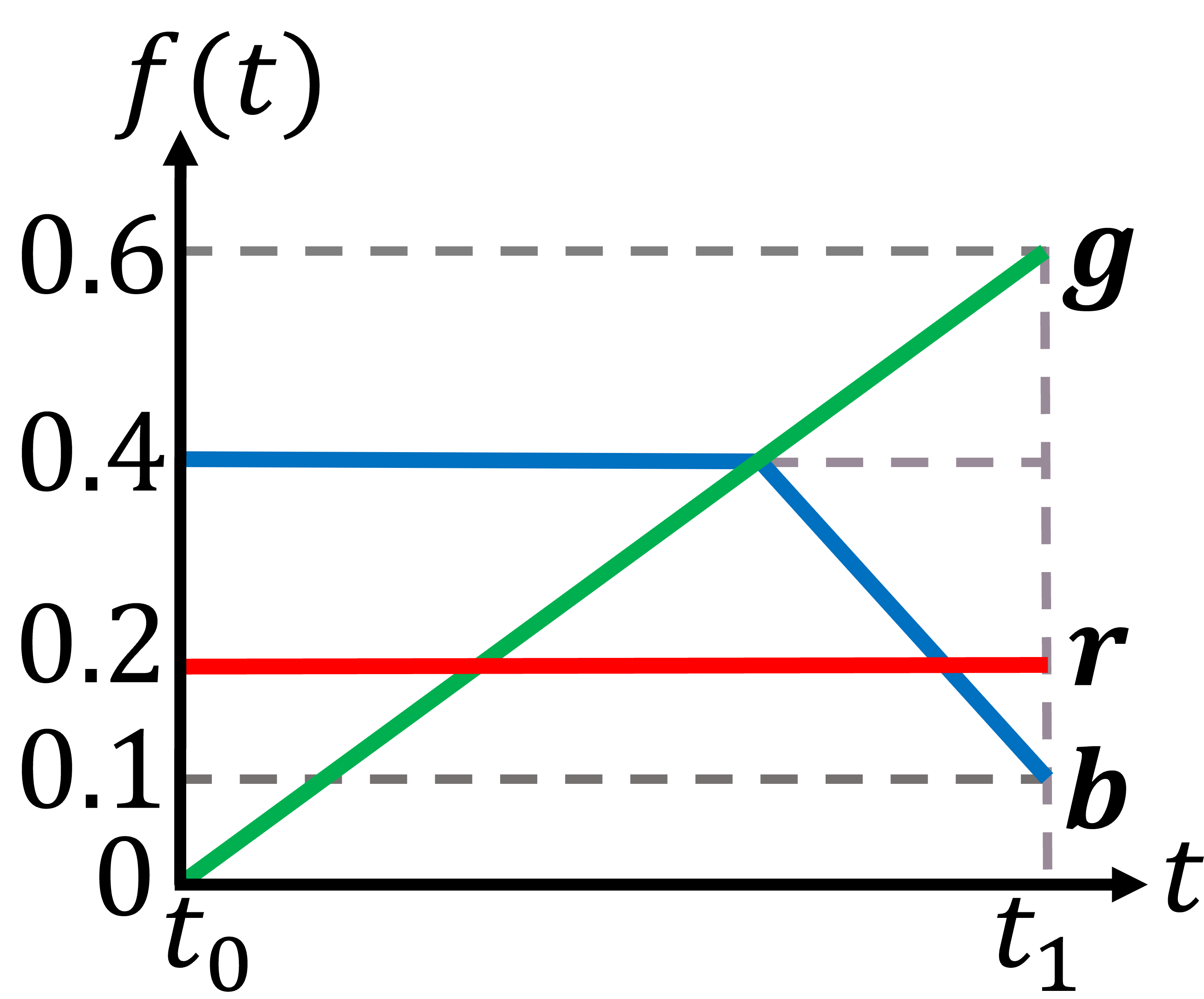
$\mathbf{f}_{l}=0.2$

$\mathbf{f}_{l}=-0.2$

linear

piecewise

rgb

Figure 7: Overview of supported target Laplacians along Poisson curves, including constant values, linear slopes, piecewise linear functions, as well as the specification of a target Laplacian per color channel.

5 Edge Graph

Diffusion curves and gradient meshes are placed and edited by the user. In order to formulate the image synthesis as a diffusion process with well-defined boundary conditions, it is necessary to subdivide the image into closed, non-overlapping regions. When one or multiple possibly-closed or nested diffusion curves intersect with a gradient mesh, it is necessary to consistently determine a Laplacian for the interior of each separate region. In the following, we utilize a planar map data structure (Gangnet et al., 1989) that we use to resolve intersections. The subsequent section will use this data structure to define connected regions and to determine a Laplacian for each region.

5.1 Definition

We introduce the undirected edge graph $(\mathcal{V},\mathcal{E})$, which consists of vertices $\mathbf{v}\in\mathcal{V}$ and edges $\mathbf{e}\in\mathcal{E}$. The set of vertices $\mathcal{V}$ contains all end points of the input boundary curves, as well as their intersections. The set of edges $\mathcal{E}$ expresses how the vertices are connected via the input boundary curves. Thereby, each edge $\mathbf{e}\in\mathcal{E}$ stores a reference to the underlying input boundary curve that it was created for, such that it can access the orientation of the input boundary curve and its boundary conditions on the left side and right side.

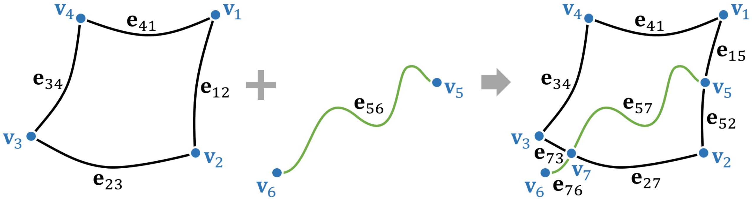
Figure 8: Given a graph with vertices $\mathcal{V}=\{\mathbf{v}_{1},\mathbf{v}_{2},\mathbf{v}_{3},\mathbf{v}_{4}\}$ and edges $\mathcal{E}=\{\mathbf{e}_{12},\mathbf{e}_{23},\mathbf{e}_{34},\mathbf{e}_{41}\}$. Inserting a new edge $\mathbf{e}_{56}$ with end points $\mathbf{v}_{5}$, $\mathbf{v}_{6}$ leads to a new node $\mathbf{v}_{7}$ at the edge intersection and a splitting of edges.

5.2 Construction

We begin with an empty graph, i.e., $\mathcal{V}=\varnothing$, $\mathcal{E}=\varnothing$. For each input boundary curve $(\mathbf{x}(t),\mathcal{B}_{l},\mathcal{B}_{r})\in\mathcal{G}\cup\mathcal{D}$ from all extended gradient meshes $\mathcal{G}$ and extended diffusion curves $\mathcal{D}$, we take the following steps:

1. Allocate two vertices $\mathbf{v}_{i}=\mathbf{x}(t_{0})$, $\mathbf{v}_{j}=\mathbf{x}(t_{1})$ and connect them by a curved edge $\mathbf{e}_{ij}$ using the curve, i.e., $\mathbf{e}_{ij}=\mathbf{x}(t)$.

2. If there is any other existing point $\mathbf{v}_{k}\in\mathcal{V}$ with $\|\mathbf{v}_{i}-\mathbf{v}_{k}\|^{2}<\epsilon$ or $\|\mathbf{v}_{j}-\mathbf{v}_{k}\|^{2}<\epsilon$, then merge nearby points.

3. If there is any other edge $\mathbf{e}_{kl}\in\mathcal{E}$ with $\mathbf{e}_{ij}\cap\mathbf{e}_{kl}\neq\varnothing$, then find the intersection and split the connected edges.

An example is given in Fig. 8. An inserted input boundary curve may have multiple intersections with other curves or with itself. The intersections are resolved by inserting vertices until no further intersections can be found. With this, the graph is brought back to a consistent state and the next input boundary curve can be processed.

5.3 Implementation Detail

During the graph construction process, input boundary curve intersections need to be calculated. To accelerate the intersection tests, we internally discretize the input boundary curves into piece-wise linear polylines in a bottom-up construction using the Ramer-Douglas-Peucker algorithm (Ramer, 1972; Douglas and Peucker, 1973). Finding curve intersections then reduces to a line-line intersection test, which we accelerate by forming a bounding volume hierarchy. When a new curve is added by the user or when the control points of an existing curve are moved, the curve is re-discretized and the bounding volume hierarchy is refit.

6 Unified Patches

Using the edge graph, we subdivide the image domain into non-overlapping patches with well-defined boundary conditions and a Laplacian in the interior. The image synthesis can then be performed for each patch independently. In the following, we explain the patch generation process.

6.1 Definition

Formally, we denote the image domain as $\mathcal{U}\subset\mathbb{R}^{2}$. Our goal is to split the image domain into connected regions $\Omega_{i}\in\mathit{\Omega}$:

$$\bigcup_{\Omega\in\mathit{\Omega}}\Omega=\mathcal{U}$$ (10)

with the requirement that for every $\Omega_{i},\Omega_{j}\in\mathit{\Omega}$ with $\Omega_{i}\neq\Omega_{j}$, the intersection of the regions $\Omega_{i}\cap\Omega_{j}\subset\mathcal{E}$ is either empty, a 0-simplex (point), or a 1-simplex (line) in the set of graph edges $\mathcal{E}$. In other words, the boundaries of regions are sections of the input boundary curves. For each region $\Omega$, we denote the desired color field as $c(\mathbf{x}):\Omega\rightarrow\mathcal{C}$ for $\mathbf{x}=(x,y)\in\Omega$, and its boundary as $\partial\Omega\subset\mathcal{E}$, which might comprise just one closed loop or multiple closed loops if there are holes inside a region. We refer to the boundary curves of a patch as patch boundary curves, which are clockwise-oriented curves with a boundary condition $\mathcal{B}$ on only the right side. Further, each patch $\Omega$ is equipped with a target Laplacian function $\mathbf{f}(\mathbf{x}):\Omega\rightarrow\mathbb{R}^{3}$ that controls the smooth color gradient inside the patch.

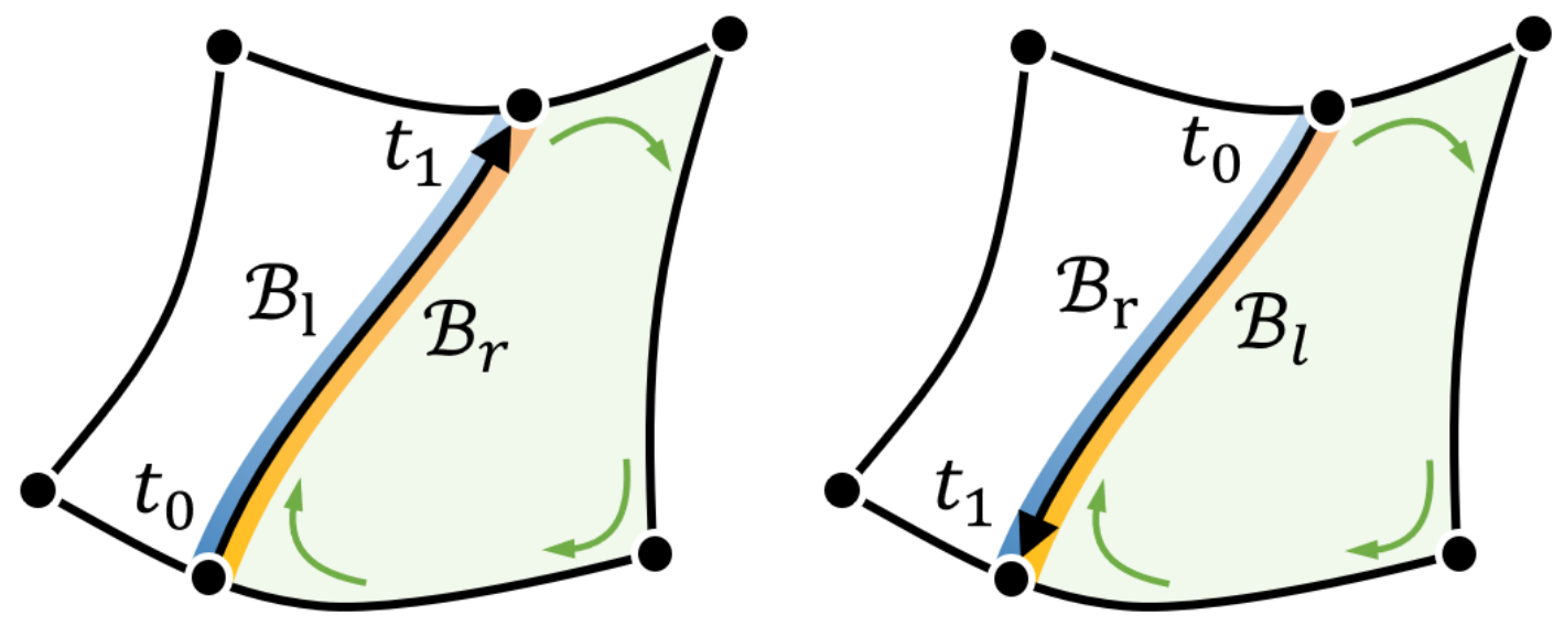
Figure 9: Each edge is associated with an underlying input boundary curve, which has an orientation (based on the parameter range $[t_{0},t_{1}]$) and a left and right boundary condition ($\mathcal{B}_{l}$, $\mathcal{B}_{r}$). When traversing the edge during construction of a patch (here green), the left or right boundary condition is chosen based on the orientation of the underlying input boundary curve.

6.2 Construction

In the following, we elaborate on how patch boundary curves and patches are created from the edge graph, and how the patch Laplacian function $\mathbf{f}(\mathbf{x})$ is defined for each patch.

Patch Boundary Curves

Each edge in the edge graph corresponds to an input boundary curve. Further, every edge is adjacent to two patches (except for image domain boundaries, where one side would be outside of the image). Thus, when constructing patches each edge will be visited up to two times when constructing patch boundary curves (once for the left side and once for the right side). The patch boundary condition $\mathcal{B}$ of a patch boundary curve is chosen from the underlying input boundary curve based on its orientation, as illustrated in Fig. 9, i.e., we choose from the left and right boundary conditions $\mathcal{B}_{l}$, $\mathcal{B}_{r}$ of the input boundary curve. Note that the two adjacent patches can be the same patch, for example, when a diffusion curve is nested inside a patch and when it is not intersecting with the outer patch boundary.

Patches

The valence $|\mathbf{v}_{i}|$ of vertex $\mathbf{v}_{i}\in\mathcal{V}$ in the graph, i.e., the number of edges connected to it, tells how often the vertex can be visited when traversing the graph in the search for closed patches, namely $2\cdot|\mathbf{v}_{i}|$ (with the exception of image boundary vertices for which it is $2\cdot|\mathbf{v}_{i}|-2$). Starting from the first vertex and its first edge in the graph, we traverse the edges from vertex to vertex tracing out a sequence of patch boundary curves that encloses a patch. A closed patch is formed by always turning right when visiting a junction, i.e., a vertex. This is illustrated in Fig. 10 (left). For the required angle measurements, the curve tangents $\dot{\mathbf{x}}(t)$ are evaluated at the end vertex of the edge, i.e., at $t_{0}$ or $t_{1}$, respectively. The edge traversal terminates when a loop was found, i.e., when the traversal returns to the start vertex. By recording how often a vertex was visited, we repeat the process until all patches are inserted and no vertex is expecting another visit.

Nested patches

A nested edge loop, as shown in Fig. 10 (right), has an interior patch boundary curve sequence, which bounds the patch that is contained by the edge loop, and an exterior patch boundary curve sequence, which denotes a patch boundary of the parent patch that contains the nested edge loop. Due to the convention of always turning right during the edge graph traversal, the two sequences are distinguished by their turning number. For all interior curve sequences, the boundary curve tangent performs a clockwise rotation (negative turning number), while the tangent of the exterior curve sequence performs a counter-clockwise rotation (positive turning number) when traversing the edge loop. For an arclength parameterized closed edge sequence $\mathbf{e}(s):[s_{0},s_{1}]\rightarrow\partial\Omega$, the integer-valued turning number is calculated by integrating the signed curvature $k(s)$ along the closed patch boundary curve:

$$\textrm{turn}(\mathbf{e}(s))=\frac{1}{2\pi}\int_{s_{0}}^{s_{1}}k(s)\,\mathrm{d}s,\;\;\textrm{with}\;\;k(s)=\frac{\mathrm{det}(\dot{\mathbf{e}}(s),\ddot{\mathbf{e}}(s))}{\|\dot{\mathbf{e}}(s)\|^{3}}.$$ (11)

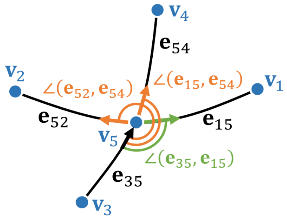
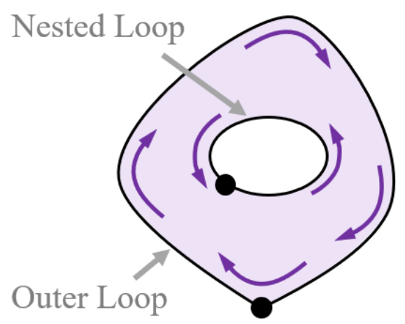
Figure 10: Left: When traversing from edge $\mathbf{e}_{35}$ to vertex $\mathbf{v}_{5}$, there are three directions, in which the traversal could continue ($\mathbf{e}_{15}$, $\mathbf{e}_{54}$, $\mathbf{e}_{52}$). Following edges, we always turn right, i.e., we select the edge with smallest angle (green). Right: When a loop is completely nested inside another loop, the patch boundaries created from the inner loop are added to the patch.

Patch Laplacian

The patch Laplacian $\mathbf{f}(\mathbf{x})$ defines the color gradient inside a patch, which is controlled by evaluating and adding the Laplacian $\mathbf{f}_{\mathbf{p}(t)}(\mathbf{x})$ of Poisson curves $\mathbf{p}(t)\in\mathcal{P}$ and by sampling the color derivatives of gradient meshes, cf. Section 2.2.

$$\mathbf{f}(\mathbf{x})=\underbrace{\sum_{\mathbf{p}(t)\in\mathcal{P}}\mathbf{f}_{\mathbf{p}(t)}(\mathbf{x})}_{\textrm{Poisson curves}}+\underbrace{\vphantom{\sum_{\mathbf{p}(t)\in\mathcal{P}}f}\left[\Delta_{\mathbf{x}}\mathbf{c}(\mathbf{u}(\mathbf{x}))\right]}_{\textrm{[Gradient mesh]}}$$ (12)

If one (and only one) patch boundary curve of a patch is part of a gradient mesh interior, we add the Laplacian of the gradient mesh $\Delta_{\mathbf{x}}\mathbf{c}(\mathbf{u}(\mathbf{x}))$, which can be evaluated analytically as explained in Appendix A (including the coordinate transformation $\mathbf{u}(\mathbf{x})$ that takes image coordinates to a $(u,v)$ coordinate in the gradient mesh). When a patch is formed from a gradient mesh, then the diffused color gradient inside the patch matches exactly the color gradient of the interpolated gradient mesh. If two gradient meshes overlap, then there is a region in which two Laplacian functions are defined. In this case, it is up to the user to decide, which Laplacian to use, for example a linear combination of both, or the one of the gradient mesh that is ’on top’, i.e., which was inserted last. To keep the implementation simple, we decided to use neither of them. Thus, if (a part of) a patch is not bound by exactly one gradient mesh, then the Laplacian of the function is only the sum of Poisson curves’s Laplacians. It there are no Poisson curves, then the patch Laplacian is homogeneous $\mathbf{f}(\mathbf{x})=\mathbf{0}$, which is equivalent to the setting for regular diffusion curves, cf. Eq. (5).

6.3 Implementation Detail

The turning number in Eq. (11) is calculated from the polyline discretization, previously described in Section 5.3, by summing up the discrete turning angles. A loop is nested inside another loop if all its discrete polyline vertices are contained. To determine containment bounding boxes are used to find candidates and a detailed check is performed by using the winding angle theorem (Jacobson et al., 2013; Spainhour et al., 2024), which is a numerically robust way of testing containment.

7 Image Synthesis

In the following, we discuss how to rasterize a patch $\Omega$ into a raster image that covers the image domain $\mathcal{U}$.

7.1 Definition

The color field $\mathbf{c}(\mathbf{x})$ of a region $\Omega$ is determined by solving a partial differential equation, i.e., a well-known Poisson problem:

$$\Delta\mathbf{c}(\mathbf{x})=\mathbf{f}(\mathbf{x}),\quad s.t.\;\;\mathcal{B}\in\partial\Omega$$ (13)

with the patch Laplacian $\mathbf{f}(\mathbf{x})$ as given by Eq. (12) and subject to the patch boundary conditions ${\mathcal{B}}$ that arise from the patch boundary curves on $\partial\Omega$, as introduced in Eqs. (7)–(8). There are many ways how the Poisson problem could be solved, including direct solvers, iterative solvers, or Monte Carlo methods. We refer to a survey (Tian and Günther, 2023) for an overview of solvers in the smooth vector graphics literature and also point out several recent solvers, which appeared after the survey (Bang et al., 2023; Sawhney et al., 2023; Sugimoto et al., 2023; Yu et al., 2024; Chen et al., 2024). Since the PDE solver is orthogonal to our contributions, we utilized a simple Jacobi relaxation for simplicity (Jeschke et al., 2009):

$$\mathbf{c}_{i,j}^{(n+1)}=\frac{\sum_{x\in\{-1,1\}}\sum_{y\in\{-1,1\}}w_{i+x,j+y}\cdot c_{i+x,j+y}^{(n)}-h^{2}\mathbf{f}_{i,j}}{w_{i+1,j}+w_{i-1,j}+w_{i,j+1}+w_{i,j-1}}$$ (14)

which iteratively calculates the pixel color $\mathbf{c}_{ij}$ for a pixel $(i,j)$ from its neighbors such that it meets the target Laplacian $\mathbf{f}_{ij}$ and where $h$ is the grid spacing of pixels in the image domain $\mathcal{U}$. The weights $w_{ij}$ are used to handle boundary conditions, which is explained in the implementation details below.

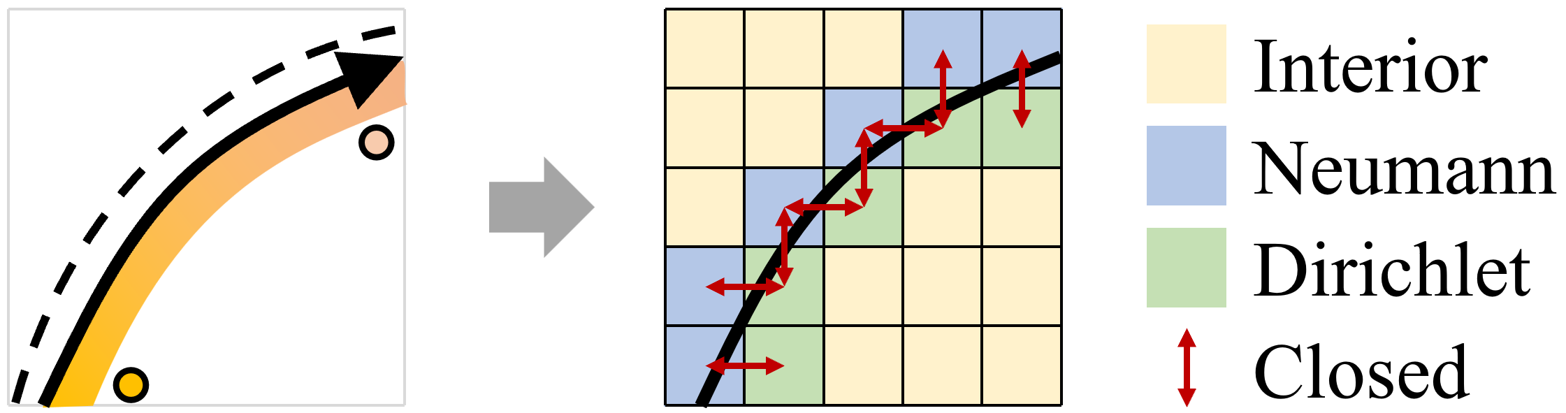
Figure 11: Left: Given is a diffusion curve with Neumann condition ($\mathcal{B}_{l}$) and Dirichlet condition ($\mathcal{B}_{r}$). Right: depiction of the pre-computed masks. We determine for each pixel, whether it is in the interior, at a Neumann boundary, or a Dirichlet boundary, which is stored in $k_{i,j}$. Further, we identify if adjacent pixels are separated (horizontally or vertically) by a patch boundary curve, and store this as binary flag in staggered grids $s^{h}_{i,j}$, $s^{v}_{i,j}$.

7.2 Implementation Detail

We implemented the Jacobi relaxation on the GPU, which requires a texture containing the target Laplacians $\mathbf{f}_{i,j}$, a texture containing the type of the pixel $k_{i,j}\in\{\textrm{interior},\textrm{Dirichlet},\textrm{Neumann}\}$, a bit mask on a staggered grid that indicates whether horizontally and vertically adjacent pixels are separated by a patch boundary curve $s^{h}_{i,j},s^{v}_{i,j}\in\{\textrm{open},\textrm{closed}\}$, and a texture that stores the final pixel color $\mathbf{c}_{i,j}$, see Fig. 11. If the pixel $(i,j)$ is a:

1. interior pixel ($k_{i,j}=\textrm{interior}$), then the weights of all adjacent pixels are set to $1$, i.e., $w_{i+1,j}=w_{i-1,j}=w_{i,j+1}=w_{i,j-1}=1$.

2. boundary pixel with Dirichlet condition ($k_{i,j}=\textrm{Dirichlet}$), then Eq. (14) is not executed. Instead, the color of the pixel is already determined by the boundary condition.

3. boundary pixel with Neumann condition ($k_{i,j}=\textrm{Neumann}$), then the weight of the adjacent pixel $w_{i+1,j}$ is set to $1$ (otherwise $0$) if it is non-separated by a patch boundary curve $s^{h}_{i,j}=\textrm{open}$ (analogous for the other neighbor pixels). This prevents color leaking over curves with Neumann condition that are contained inside a patch, see for example Fig. 5.

We identify if a pixel is a boundary pixel in a pre-process by determining the pixels that belong to the patch using the winding angle theorem (Jacobson et al., 2013), and flag pixel $(i,j)$ as boundary if one of its neighbors $(i+1,j)$, $(i-1,j)$, $(i,j+1)$, $(i,j-1)$ is not in the patch, or if a ray cast between adjacent pixels intersects a patch boundary curve. We determine the closest patch boundary curve and set the pixel type $k_{i,j}$ and the openness $s_{n}$, $s_{e}$, $s_{s}$, $s_{w}$ accordingly. If the pixel has a Dirichlet condition, then we set $\mathbf{c}_{i,j}$ according to the closest hit location on the patch boundary curve. If the Dirichlet condition originated from an input boundary curve that belonged to a gradient mesh, then we interpolate the pixel color in the gradient mesh at the location of the pixel center $(i,j)$, rather than taking the color on its boundary curve. The texture with the target Laplacian $\mathbf{f}_{i,j}$ is set by evaluating the gradient mesh Laplacian $\Delta_{\mathbf{x}}\mathbf{c}(\mathbf{u}(\mathbf{x}))$ (if a gradient mesh was contained, cf. Eq. (12)), and the Laplacians $\mathbf{f}_{\mathbf{p}(t)}$ of Poisson curves $\mathbf{p}(t)$ are additively rasterized on top.

8 Results

In the following section, we present our results using scenes that contain gradient meshes, diffusion curves, and Poisson curves. We made all test scenes available online (Tian and Günther, 2024). All images are rendered at a resolution of $1024\times 1024$.

(a) input meshes

(b) input curves

(c) undirected edge graph

(d) unified patch representation

(e) final synthesized image

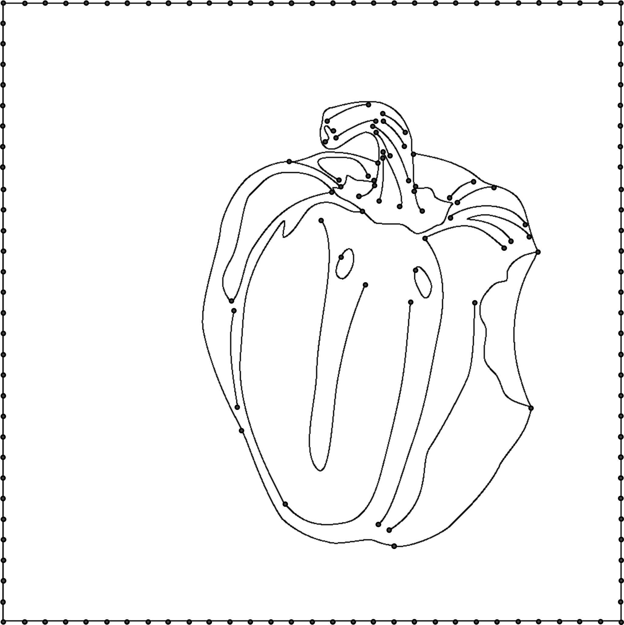
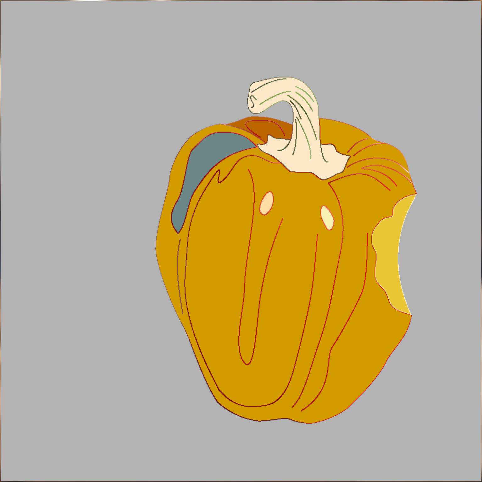
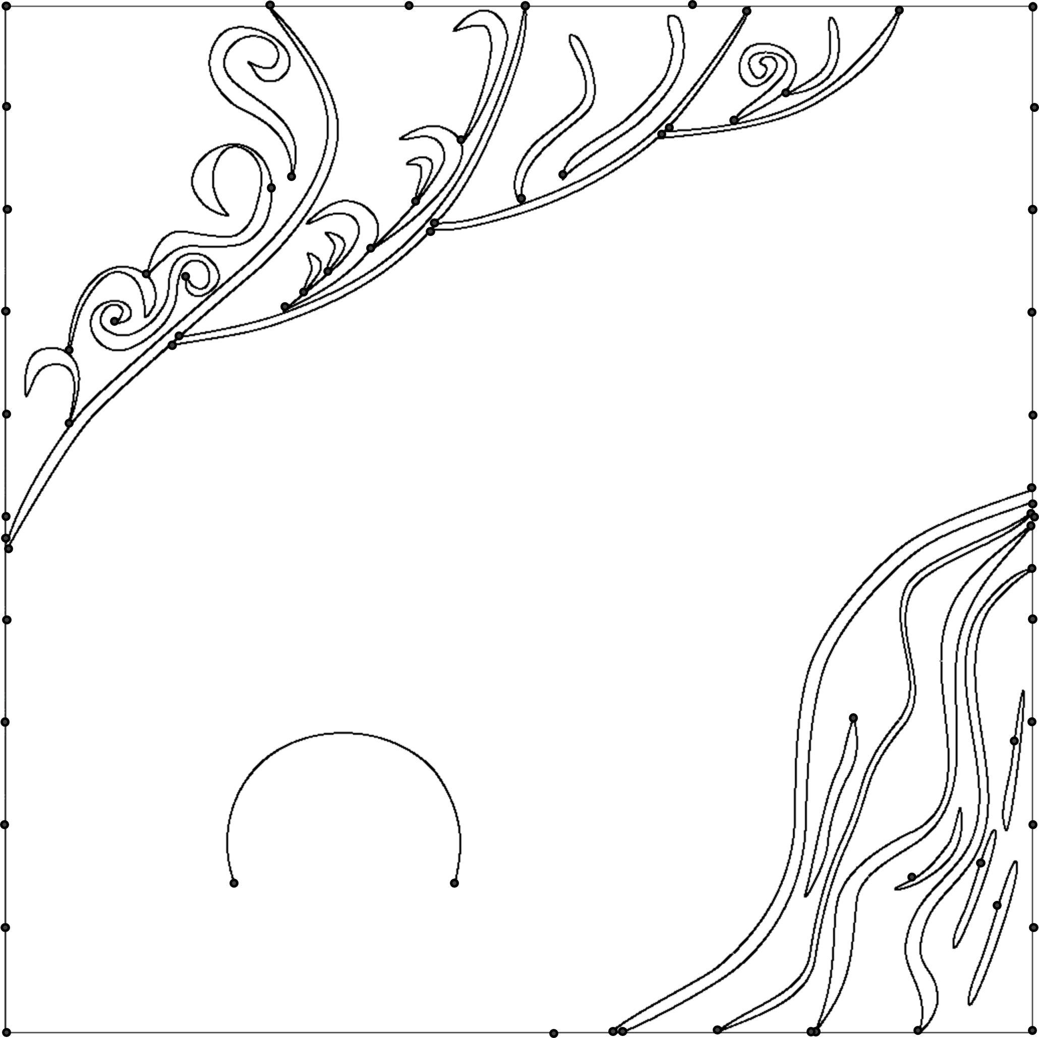
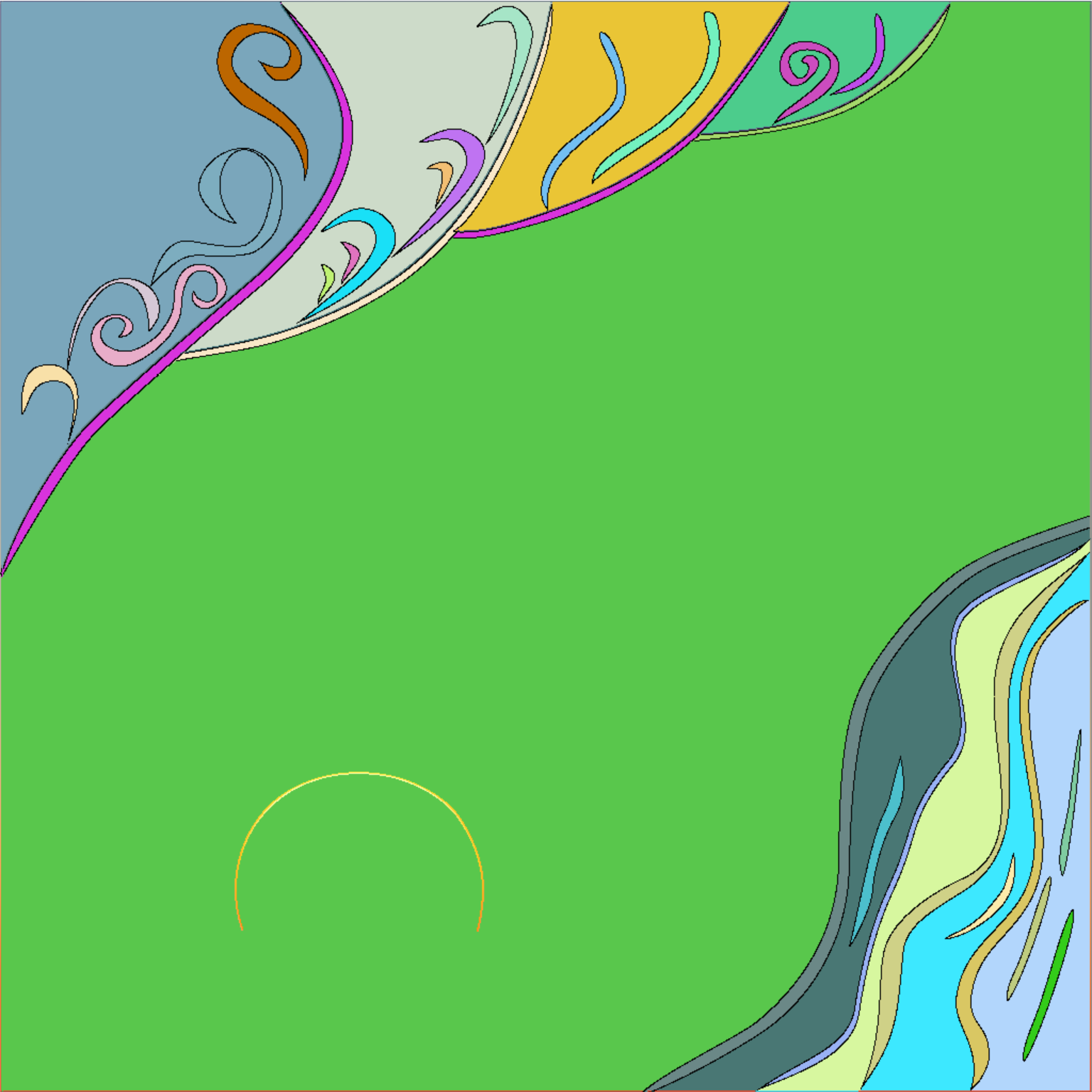
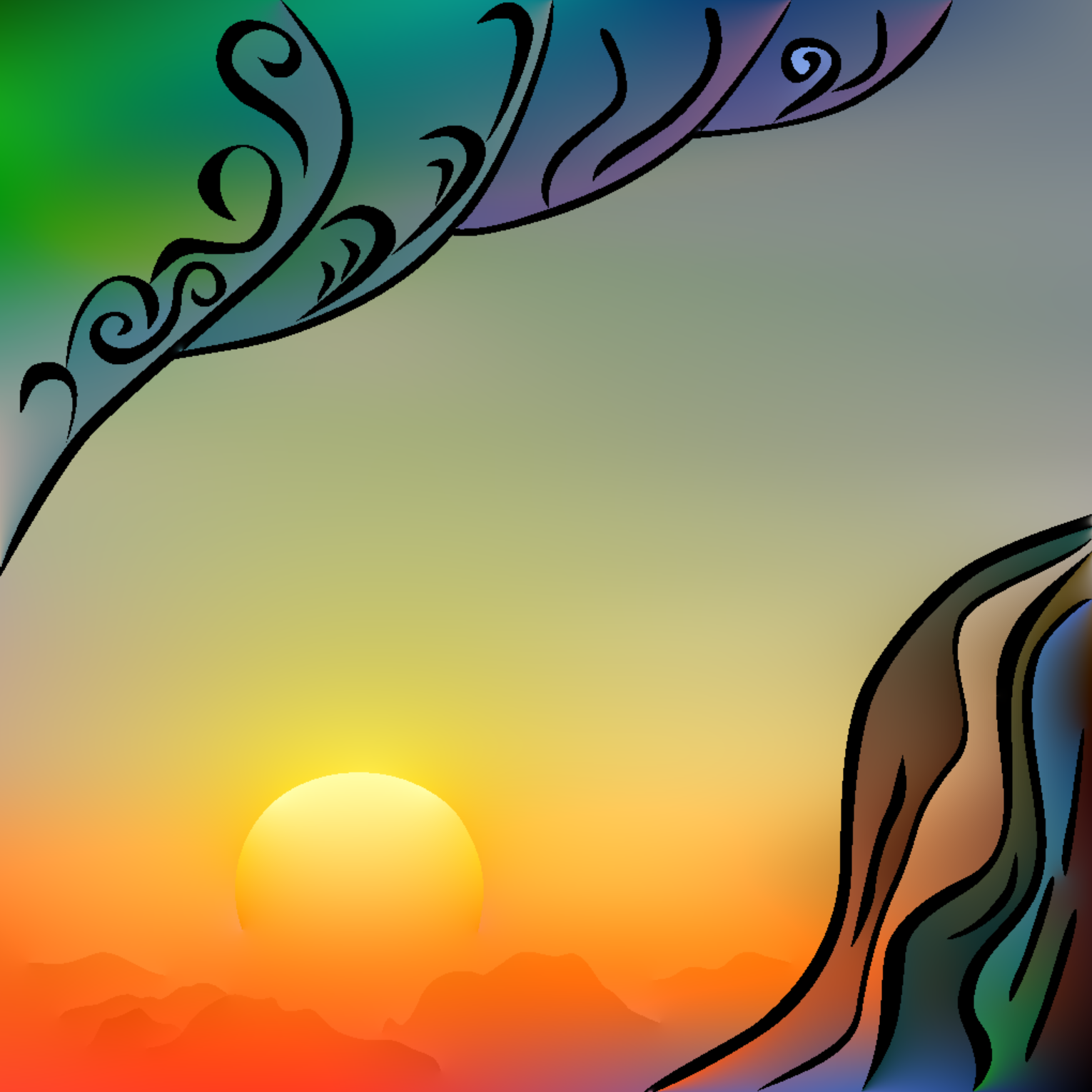
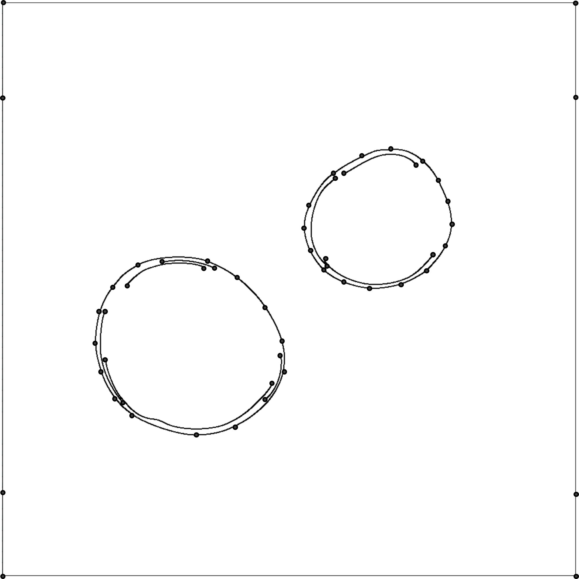
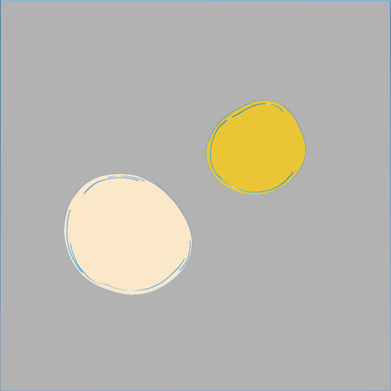
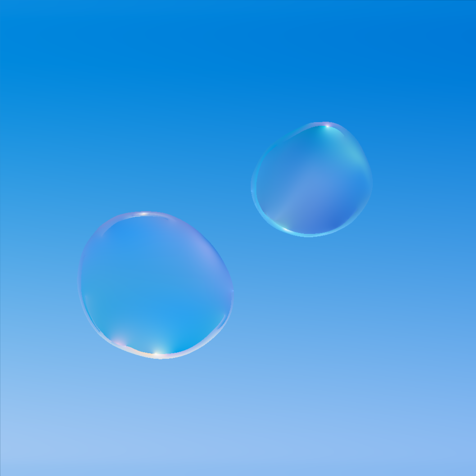
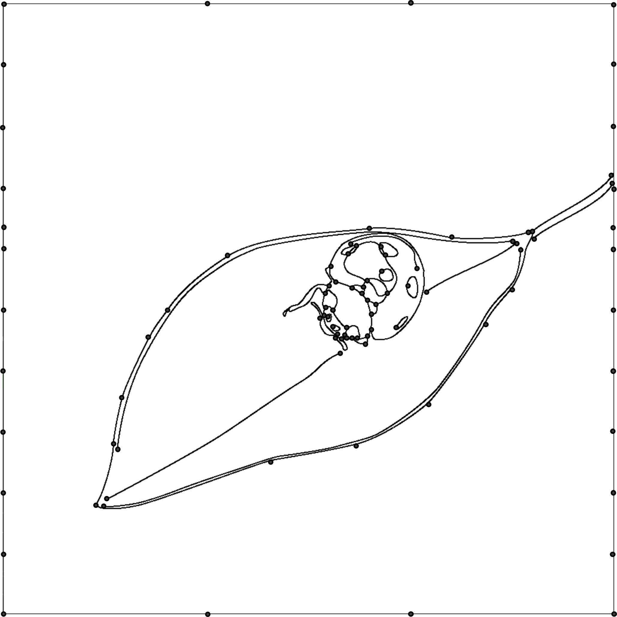
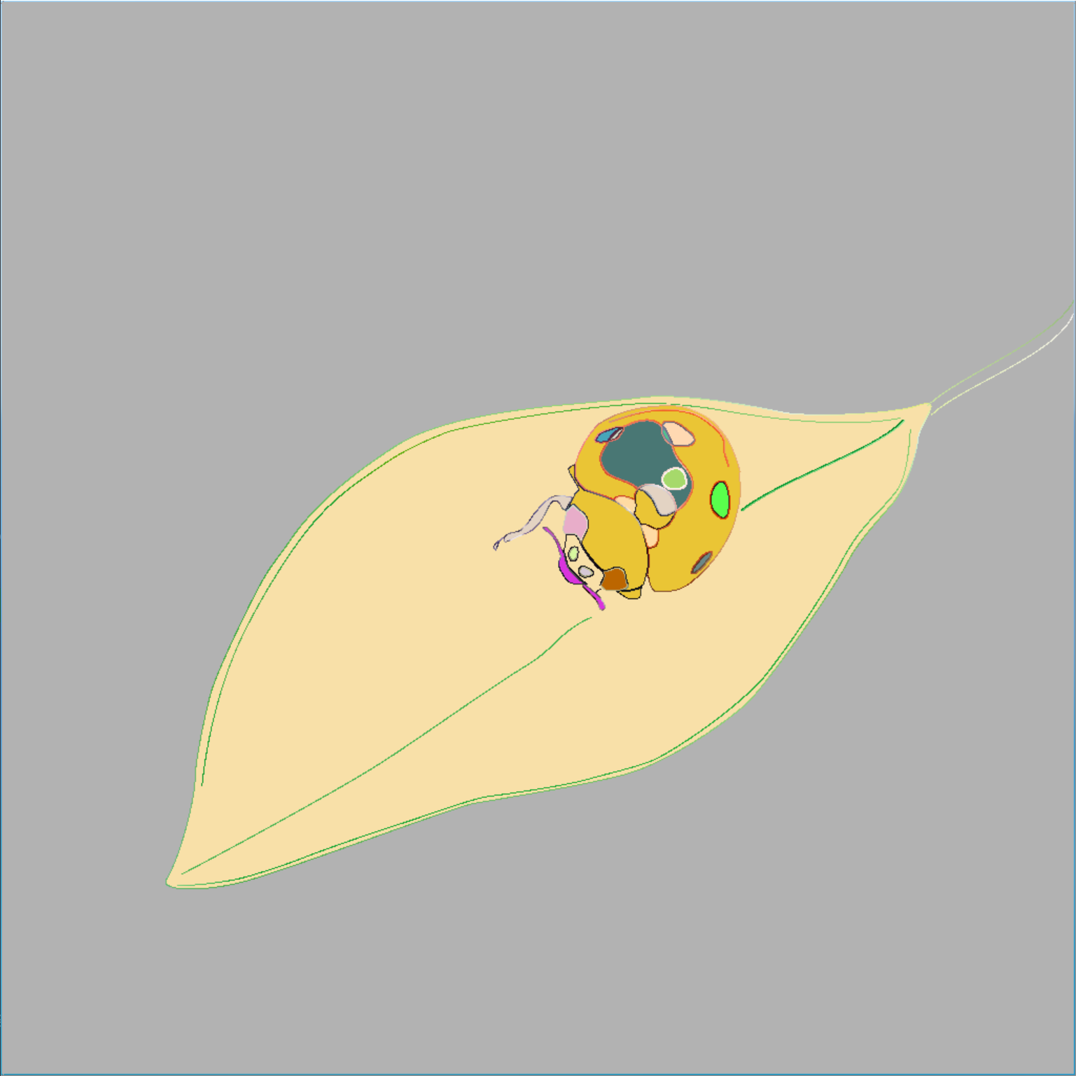
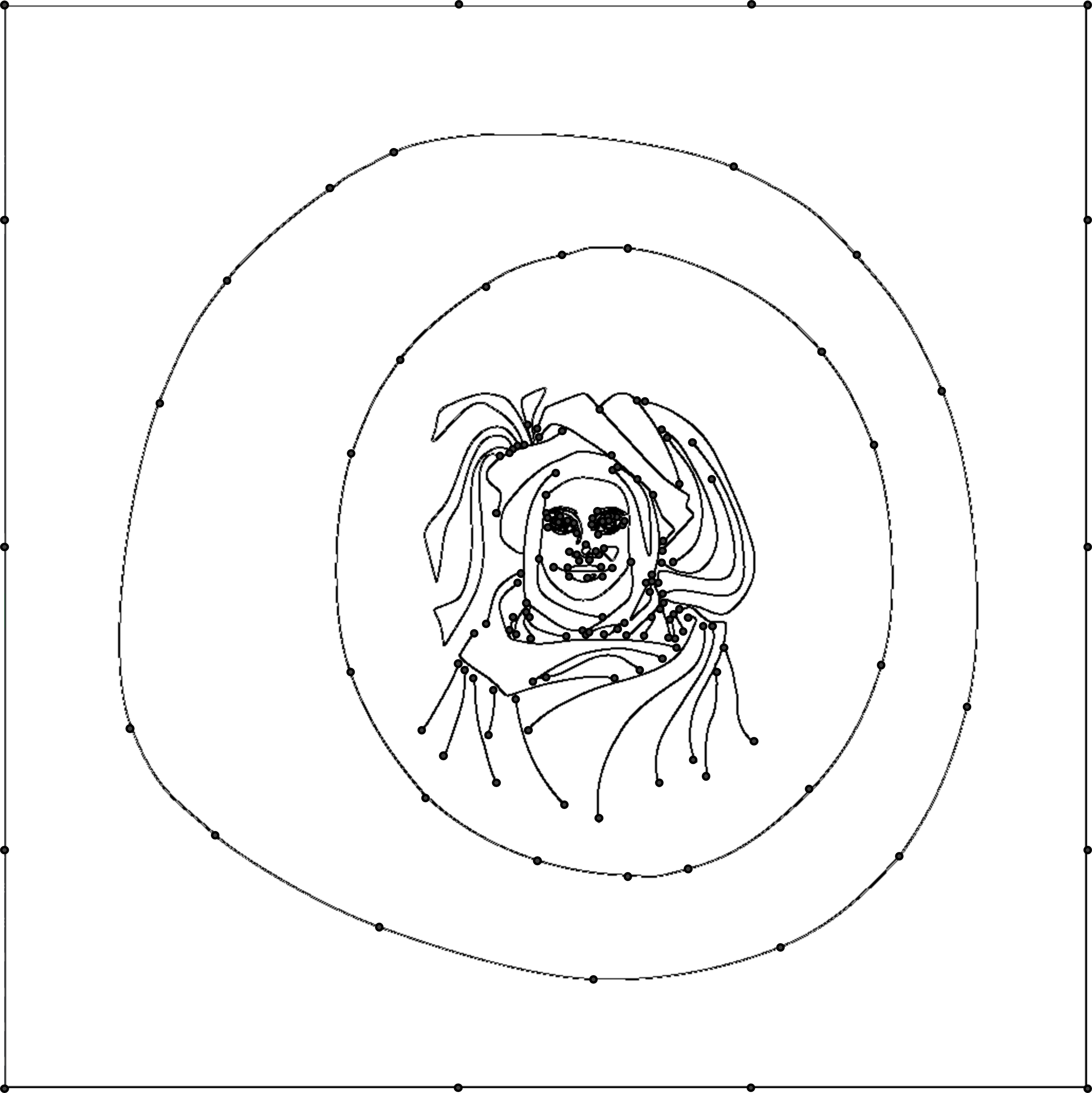
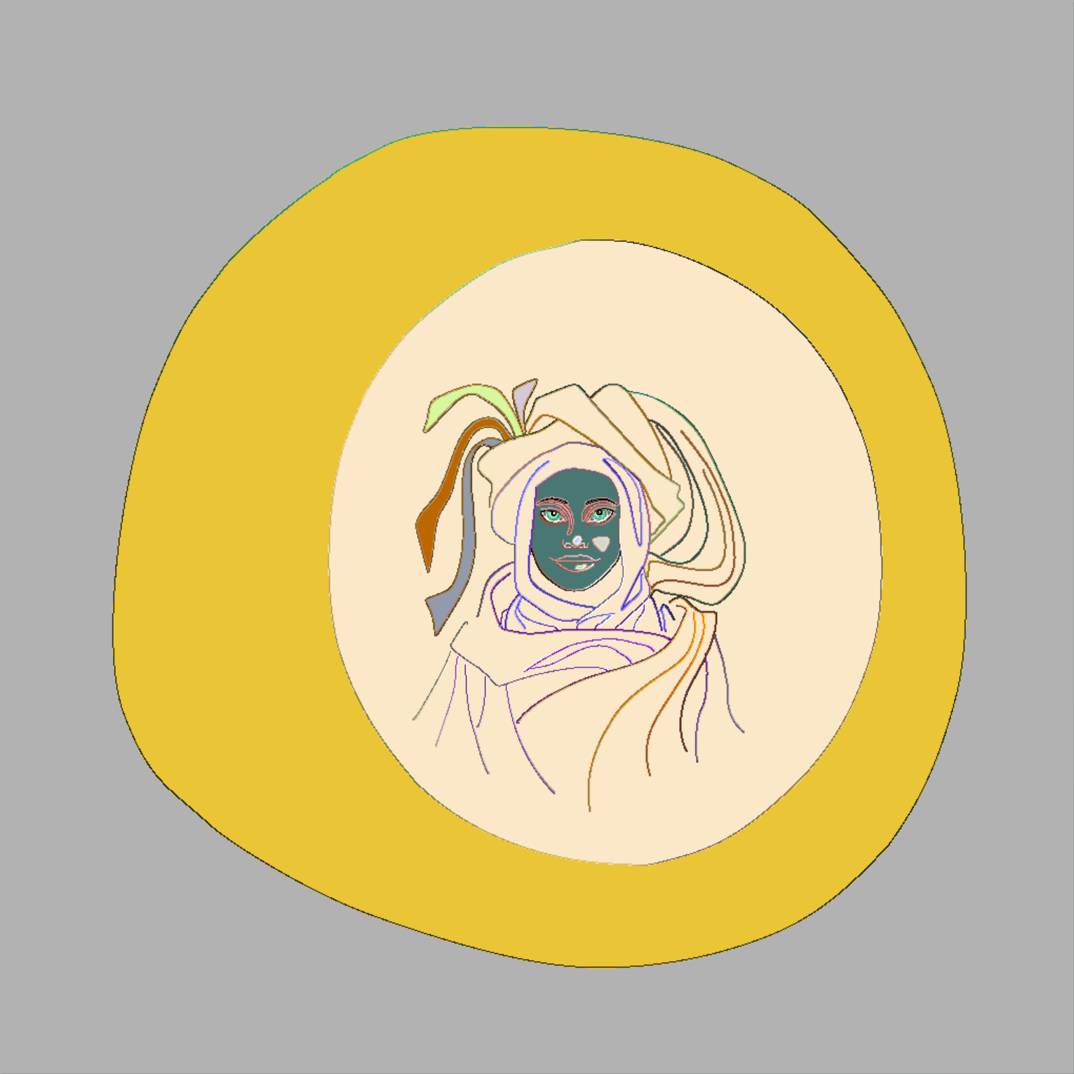
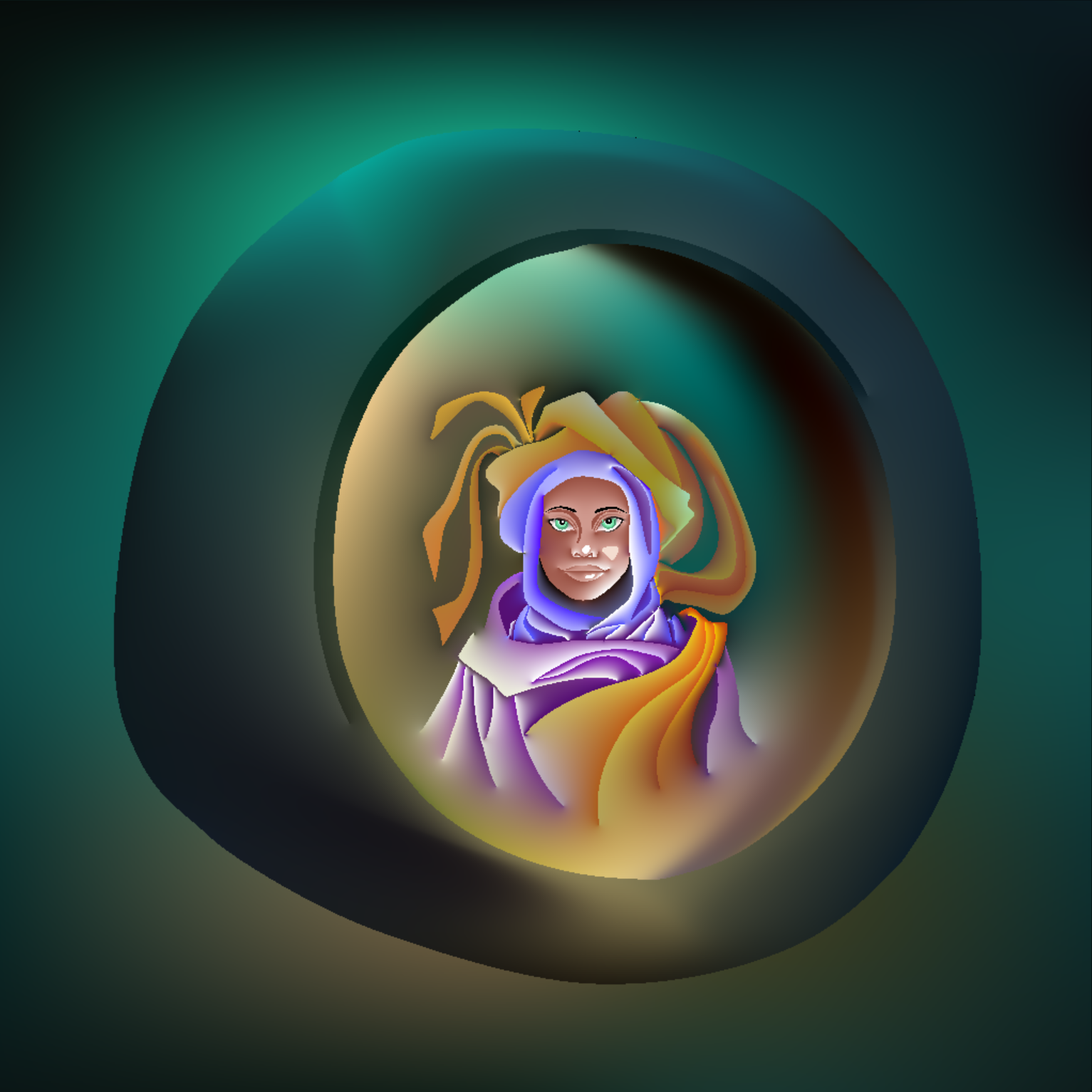
Figure 12: Qualitative results of the pepper, sunset, bubbles, ladybug, and portal scene. From left to right, we show the input primitives (a) and (b), the undirected edge graphs (c), the unified patch representations (d) that were formed by our algorithm and the final rendering results (e).

8.1 Qualitative Results

We begin with a description of the test scenes. For all test scenes, the input meshes and curves, the undirected edge graph, our unified patch representation, and the final rendering result are shown. To illustrate the input primitives, we depict the gradient mesh control polygon with solid lines, where different colors are applied for each mesh. Input boundary curves are shown as double-sided curve with an illustration of the respective boundary condition on the left and right. Dirichlet conditions directly show the corresponding color, while Neumann conditions are illustrated with a dash-dot pattern. Poisson curves are visualized with a long dash pattern. The undirected edge graph is visualized by solid black curves and the vertices are depicted with black circles. Note that Poisson curves are not part of the edge graph, since they are rendered additively onto the target Laplacian function. The unified patch representation gives all pixels that belong to the same region a common color. The colors are assigned from a custom color table such that the regions are visually distinguishable. The color is not related to the image content. The last column shows the final result.

Crane

Inspired from an ancient Chinese painting (the Auspicious Cranes by Emperor Huizong), we modeled a crane with diffusion curves, which is shown in Fig. 1. The boundary of the crane is largely modeled with Neumann conditions. We modeled the clouds with two $3\times 4$ gradient meshes. In addition, we added diffusion curves and Poisson curves on the gradient meshes for the layered and detailed effects of clouds. The background is formed from a $3\times 3$ gradient mesh that mimics the similar color transition of the inspirational image. The image was rendered using 1 k Jacobi iterations.

Pepper

Fig. 12 (first row) shows an extension of the poivron scene from Orzan et al. (2008). We replaced the background with a $30\times 30$ gradient mesh that was fitted with Adobe Illustrator to a photograph inside a restaurant. The gradient mesh’s smoothness creates the impression of defocus blur, putting emphasis on the pepper in the foreground. We took a bite out of the pepper by adding further diffusion curves. The outer boundary of the pepper is modeled with homogeneous Neumann conditions, such that it can be placed in the scene without causing color diffusion into the background. The shadow on the table is modeled with Poisson curves. The background contains many color gradients, which would have been cumbersome to model with diffusion curves only. To render the image we performed 10 k Jacobi iterations using Eq. (14).

Sunset

Fig. 12 (second row) shows a colorful sunset. The color gradient in the background contains multiple hues and is modeled with a $10\times 3$ gradient mesh. We also deformed the spatial control points for artistic effects. Since it is interrupted by other curve primitives in-between, the color gradient would have been difficult to model with diffusion curves only. The sun is drawn using a diffusion curve, which allows for the modeling of the faint glow due to scattering. The sun diffuses its light into the background. On the top and bottom of the image, we placed diffusion curves that contrast the nature background with expressive wavy shapes. This image was rendered using 15 k Jacobi iterations.

Bubbles

In Fig. 12 (third row), we modeled two soap bubbles. We used a $1\times 3$ gradient mesh to model the background sky for smooth color transitions. The bubbles are created by two $4\times 4$ gradient meshes. The smooth color transitions are difficult to model directly with diffusion curves. This example shows that a vivid scene can be represented by a small number of primitives when combining mesh-based and curve-based methods. We rendered the image with 15 k Jacobi iterations.

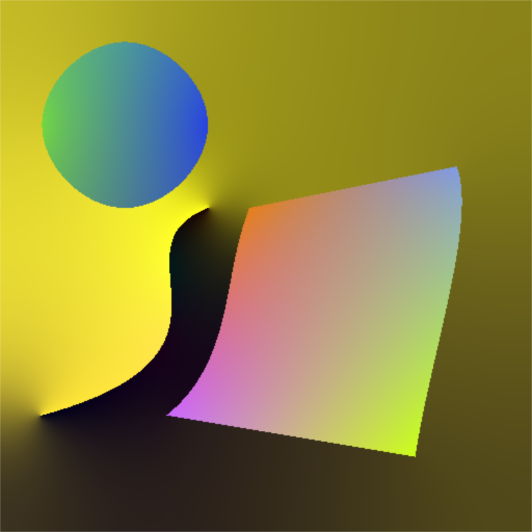
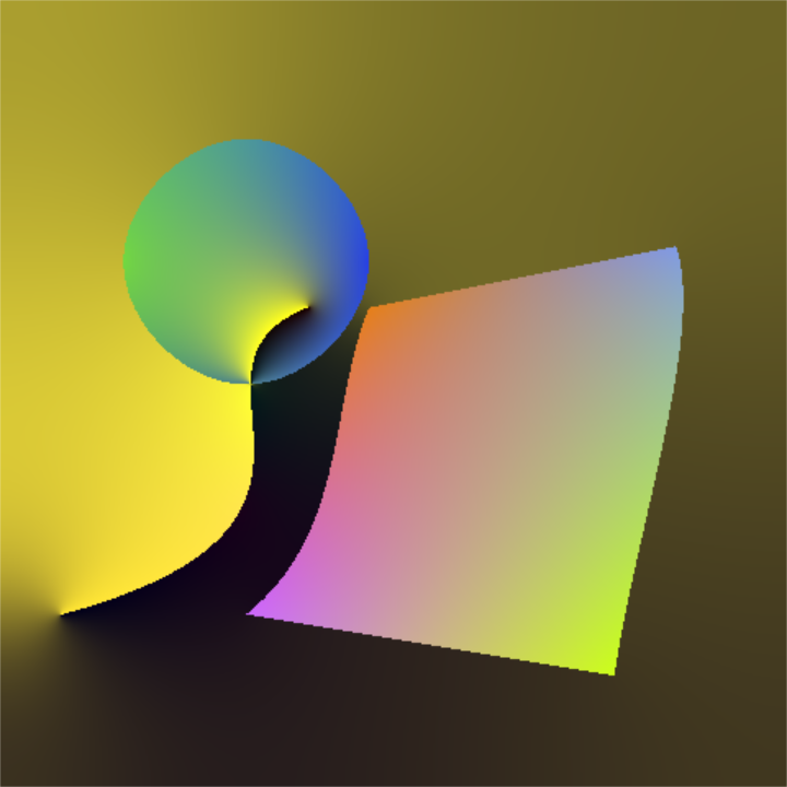
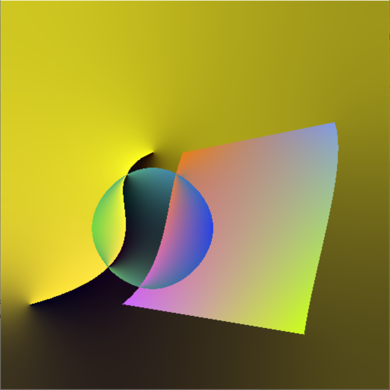
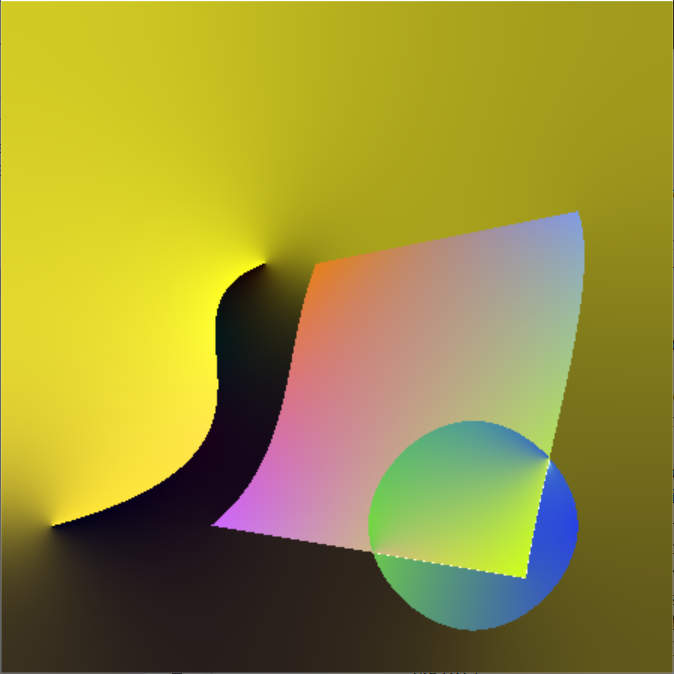
Figure 13: During user interaction, new patches are formed and destroyed. To achieve a consistent scene editing experience, the user only edits input gradient meshes, diffusion curves, and Poisson curves. The edge graph and the unified patches are not exposed to the user and are created fully automatically.

Table 1: Performance measurements for the various test scenes used in the paper. The columns list the corresponding figure, the number of input diffusion curves (#DC), the number of input Poisson curves (#PC), the number of input gradient meshes (#GM) for which we list the grid resolution in brackets, the number of vertices (#V) and edges (#E) in the edge graph, the number of patches (#P), the computation time to form the edge graph, the computation time to traverse the edge graph, and the time needed to resolve the nesting of patches. All timings are in milliseconds.

Scene	Figure	#DC	#PC	#GM	#V	#E	#P	Construct graph	Trav. graph	Create patches
Crane	Fig. 1	68	5	3	160	124	8	16	5	13
Pepper	Fig. 12 (first row)	36	3	1	184	165	8	11	9	12
Sunset	Fig. 12 (second row)	38	6	1	88	108	37	16	2	7
Bubble	Fig. 12 (third row)	9	0	3	62	53	3	2	1	1
Ladybug	Fig. 12 (fourth row)	59	8	2	111	113	20	14	2	16
Portal	Fig. 12 (fifth row)	87	1	3	211	167	17	20	3	14

Ladybug

The test scene in Fig. 12 (fourth row) is based on the ladybug diffusion curve model of Orzan et al. (2008). We made minor adjustments to the original curve endpoints to remove edge crossings that would otherwise cause color leakage. In addition, we set the outer boundary of the ladybug to Neumann condition. We placed the ladybug in a beach scene, which contains an ocean and a blue sky. The background is modeled using a $11\times 3$ gradient mesh. In addition, we model a leaf on which the ladybug sits with a $6\times 2$ gradient mesh, which captures the subtle color changes without smoothing. The leaf veins are created with Poisson curves, and the outer boundary is modeled with diffusion curves to add a scattering effect. We rendered the image using 2 k Jacobi iterations.

Portal

The last test scene in Fig. 12 (fifth row) shows a portal. We created the portal with three gradient meshes: a $4\times 3$ background mesh, and two $3\times 4$ gradient meshes for the outer and internal parts of the portal. The rendered portal contains smooth color transitions to represent light and shadows. Inside the portal, We modified the zephyr diffusion curve model of Orzan et al. (2008). The diffusion curves diffuse color into the portal. The mesh Laplacian provides richer effects and more potential for artistic control compared to curve-only results. The image was rendered using 15 k Jacobi iterations.

8.2 User Interaction

When individual input primitives are moved in the scene by the user during editing, intersections with other primitives will occur that lead to the creation of new patches or the disappearance of other patches. To ensure a consistent editing experience, we made sure that all user input is specified on the extended gradient meshes, extended diffusion curves, and Poisson curves alone. On the front end, the user is not accessing the edge graph or the patch representation, which are both computed fully automatically from the input primitives. Fig. 13 shows the rendered output when taking a closed diffusion curve and moving it across a scene. Intersections with other diffusion curves and gradient meshes are created, which causes new patches to form or disappear. Using our data structures, the rendering results remain consistent throughout the editing process.

8.3 Performance Analysis

We evaluated our method on an Intel Core i9-10980XE with 4.6 Ghz and an Nvidia RTX 2080 TI GPU. The performance measurements are reported in Table 1. To give context we report for each scene statistics about the complexity of the input data (number of diffusion curves, number of Poisson curves, number of gradient meshes), statistics on the complexity of the edge graph (number of vertices and edges), and the number of patches in our patch representation. We report the time it takes to compute the edge graph, the time it takes to traverse the edge graph during the patch construction, and the time it takes to resolve the nesting relationships.

Across all test scenes, the edge graph construction was at around 12-17 ms, the edge graph traversal at 4-10 ms, and the patch creation at 13-45 ms. In sum, we achieved across all scenes an interactive frame rate (29-67 milliseconds per frame). Resolving the nested patches is currently the bottleneck, since it requires the traversals to determine the clockwise/anti-clockwise turn numbers in Eq. (11) and the test whether patches are fully contained within each other. While we incorporated bounding volume hierarchies to accelerate the tests, we think that further improvements for the future could include partial updates of both the edge graph and the patch representation whenever an object moves. Further, a hierarchical discretization could be used to accelerate the winding angle tests. Despite us rebuilding the graph and patches from scratch, we still obtained interactive results.

8.4 Discussion

The edge graph and our resulting patch construction directly depend on the quality of the input primitives. If the input primitives contain tiny gaps or small crossings, then a corresponding patch representation would carry on those artifacts. In recent years, more exact vector graphics rendering algorithms have been developed and utilized, such as Walk-on-Spheres (Sawhney and Crane, 2020), Walk-on-Boundaries (Sugimoto et al., 2023), or Walk-on-Stars (Sawhney et al., 2023). These approaches likewise suffer from inaccuracies in the scene description, since they are able to resolve the color transport through narrow gaps. More research towards automatic input cleaning or user interfaces that naturally steer the user towards more accurate scene descriptions would be helpful for both scene modeling and rendering.

9 Conclusions

In this paper, we unified the mathematical modeling of mesh-based vector graphics and curve-based vector graphics, which allows for the first time to include both types of primitives in the same scene. For this, we rephrased the interpolation inside gradient meshes as solution to a Poisson problem by searching for a color field that matches the Laplacian of the gradient mesh. We developed a four-stage pipeline that takes gradient meshes, diffusion curves, and Poisson curves as input. First, we extended gradient meshes and diffusion curves by enabling the specification of Neumann conditions in addition to the usual Dirichlet conditions. Second, our approach handles arbitrary intersections of diffusion curves and gradient meshes, since all intersections are resolved through the construction of an edge graph. Third, from the edge graph, non-overlapping patches with well-defined boundary conditions and a target Laplacian are derived. Fourth, a standard Poisson problem is solved in the interior of each patch to synthesize the output image. Our pipeline is free of parameters and the final rasterized images can be computed with any off-the-shelf Poisson solver.

In the past, research on mesh-based and curve-based smooth vector graphics followed independent research threads, which concentrated on the editing, rasterization, or vectorization of the individual primitives. We hope that the unified treatment will spur further research that promotes synergies of the two approaches, for example regarding novel image synthesis or vectorization methods. The next step in the generalization will include the incorporation of bi-harmonic diffusion curves (Finch et al., 2011), for which harmonic solutions can be searched in the Laplacian domain. Similar to common content creation tools, it could be useful to introduce multiple layers of smooth vector graphics.

Appendix A Laplacian of Gradient Mesh

Gradient meshes consist of one or multiple Ferguson patches, each containing bi-cubic color patches, whose Laplacian is not necessarily homogeneous. In fact, the ability to add more variation to the color gradient is what makes gradient meshes artistically expressive. In the following, we let $\mathbf{u}=(u,v)\in[0,1]^{2}$ be the UV coordinate that parameterizes a single Ferguson patch with colors $\mathbf{c}(\mathbf{u})$ and 2D spatial coordinates $\mathbf{x}(\mathbf{u})$, following Eq. (4). Since a Ferguson patch is parameterized in UV coordinates $\mathbf{u}$ and since our Poisson equation in Eq. (13) is in spatial coordinates $\mathbf{x}$, coordinate transformations are needed, including the mapping from $\mathbf{x}$ to $\mathbf{u}$ and its coordinate partials, as well as the gradient and the Laplacian of color with respect to $\mathbf{x}$, as explained in the following.

Pre-Image

The pre-image from image space coordinates $\mathbf{x}$ back to $\mathbf{u}$ is later for simplicity referred to as $\mathbf{u}(\mathbf{x})$. The pre-image exists if the coordinates $\mathbf{x}(\mathbf{u})$ do not contain folds, i.e., if $\mathbf{x}(\mathbf{u})$ is a homeomorphism. Inside that function, we find the $\mathbf{u}_{0}$ coordinate that maps to image space coordinate $\mathbf{x}_{0}$ by solving the root finding problem $\mathbf{x}(\mathbf{u}_{0})-\mathbf{x}_{0}=\mathbf{0}$. Thus, given an image space coordinate $\mathbf{x}$, we can evaluate the color of a Ferguson patch at the corresponding UV coordinate via $\mathbf{c}(\mathbf{u}(\mathbf{x}))$.

Coordinate Jacobian

The partial derivatives of the inverse coordinate transformation are for $\mathbf{x}(\mathbf{u})=(x(u,v),y(u,v))^{\mathrm{T}}$:

$$\begin{pmatrix}\frac{\partial}{\partial x}u&\frac{\partial}{\partial x}v&0&0&0\\ \frac{\partial}{\partial y}u&\frac{\partial}{\partial y}v&0&0&0\\ \frac{\partial^{2}}{\partial x^{2}}u&\frac{\partial^{2}}{\partial x^{2}}v&\frac{\partial}{\partial x}u\frac{\partial}{\partial x}u&\frac{\partial}{\partial x}v\frac{\partial}{\partial x}v&2\frac{\partial}{\partial x}u\frac{\partial}{\partial x}v\\ \frac{\partial^{2}}{\partial y^{2}}u&\frac{\partial^{2}}{\partial y^{2}}v&\frac{\partial}{\partial y}u\frac{\partial}{\partial y}u&\frac{\partial}{\partial y}v\frac{\partial}{\partial y}v&2\frac{\partial}{\partial y}u\frac{\partial}{\partial y}v\\ \frac{\partial^{2}}{\partial x\partial y}u&\frac{\partial^{2}}{\partial x\partial y}v&\frac{\partial}{\partial x}u\frac{\partial}{\partial y}u&\frac{\partial}{\partial x}v\frac{\partial}{\partial y}v&\frac{\partial}{\partial x}u\frac{\partial}{\partial y}v+\frac{\partial}{\partial y}u\frac{\partial}{\partial x}v\end{pmatrix}$$ (15)

$$= \begin{pmatrix}\frac{\partial}{\partial u}x&\frac{\partial}{\partial u}y&0&0&0\\ \frac{\partial}{\partial v}x&\frac{\partial}{\partial v}y&0&0&0\\ \frac{\partial^{2}}{\partial u^{2}}x&\frac{\partial^{2}}{\partial u^{2}}y&\frac{\partial}{\partial u}x\frac{\partial}{\partial u}x&\frac{\partial}{\partial u}y\frac{\partial}{\partial u}y&2\frac{\partial}{\partial u}x\frac{\partial}{\partial u}y\\ \frac{\partial^{2}}{\partial v^{2}}x&\frac{\partial^{2}}{\partial v^{2}}y&\frac{\partial}{\partial v}x\frac{\partial}{\partial v}x&\frac{\partial}{\partial v}y\frac{\partial}{\partial v}y&2\frac{\partial}{\partial v}x\frac{\partial}{\partial v}y\\ \frac{\partial^{2}}{\partial u\partial v}x&\frac{\partial^{2}}{\partial u\partial v}y&\frac{\partial}{\partial u}x\frac{\partial}{\partial v}x&\frac{\partial}{\partial u}y\frac{\partial}{\partial v}y&\frac{\partial}{\partial u}x\frac{\partial}{\partial v}y+\frac{\partial}{\partial v}x\frac{\partial}{\partial u}y\end{pmatrix}^{-1}$$ (16)

Gradient

The spatial color gradient follows from the chain rule:

$$\frac{\partial\mathbf{c}(\mathbf{u}(\mathbf{x}))}{\partial\mathbf{x}}=\frac{\partial c(\mathbf{u}(\mathbf{x}))}{\partial\mathbf{u}}\frac{\partial\mathbf{u}(\mathbf{x})}{\partial\mathbf{x}}.$$ (17)

Laplacian

The Poisson problem in Eq. (13) requires the Laplacian of color with respect to image space $\Delta_{\mathbf{x}}\mathbf{c}(\mathbf{u}(\mathbf{x}))$, which is likewise computed via chain rule:

$$\Delta_{\mathbf{x}}\mathbf{c}(\mathbf{u}(\mathbf{x})) =\frac{\partial^{2}\mathbf{c}(\mathbf{u}(\mathbf{x}))}{\partial x^{2}}+\frac{\partial^{2}\mathbf{c}(\mathbf{u}(\mathbf{x}))}{\partial y^{2}}$$ (18)

$$=\frac{\partial\mathbf{u}(\mathbf{x})}{\partial x}^{\mathrm{T}}\,\frac{\partial^{2}\mathbf{c}(\mathbf{u}(\mathbf{x}))}{\partial\mathbf{u}^{2}}\,\frac{\partial\mathbf{u}(\mathbf{x})}{\partial x}+\frac{\partial\mathbf{c}(\mathbf{u}(\mathbf{x}))}{\partial\mathbf{u}}^{\mathrm{T}}\frac{\partial^{2}\mathbf{u}}{\partial x^{2}}$$ (19)

$$+\frac{\partial\mathbf{u}(\mathbf{x})}{\partial y}^{\mathrm{T}}\,\frac{\partial^{2}\mathbf{c}(\mathbf{u}(\mathbf{x}))}{\partial\mathbf{u}^{2}}\,\frac{\partial\mathbf{u}(\mathbf{x})}{\partial y}+\frac{\partial\mathbf{c}(\mathbf{u}(\mathbf{x}))}{\partial\mathbf{u}}^{\mathrm{T}}\frac{\partial^{2}\mathbf{u}}{\partial y^{2}}.$$ (20)

Using the above ingredients, we can now add the Laplacian of each Ferguson patch of a gradient mesh $\Delta_{\mathbf{x}}\mathbf{c}(\mathbf{u}(\mathbf{x}))$ to the patch Laplacian $\mathbf{f}(\mathbf{x})$, see Eq. (12). The symbolic derivatives as described above are an alternative to the numerical computation via finite differences from a rasterized gradient mesh image. Unlike symbolic derivatives, the error of the numerical computation depends on the image resolution. The symbolic derivatives could also be useful for differentiable rasterizers that might be employed in the future for automatic vectorization.

References

- Hsiao et al. (2023) Kai-Wen Hsiao, Yong-Liang Yang, Yung-Chih Chiu, Min-Chun Hu, Chih-Yuan Yao, and Hung-Kuo Chu. Img2Logo: Generating golden ratio logos from images. Computer Graphics Forum (Proc. Eurographics), 42(2):37–49, 2023. ISSN 1467-8659. doi:10.1111/cgf.14742.
- Sun et al. (2007) Jian Sun, Lin Liang, Fang Wen, and Heung-Yeung Shum. Image vectorization using optimized gradient meshes. ACM Transactions on Graphics (TOG), 26(3):11–es, 2007. doi:10.1145/1276377.1276391.
- Lai et al. (2009) Yu-Kun Lai, Shi-Min Hu, and Ralph R Martin. Automatic and topology-preserving gradient mesh generation for image vectorization. ACM Transactions on Graphics (TOG), 28(3):1–8, 2009. doi:10.1145/1531326.1531391.
- Orzan et al. (2008) Alexandrina Orzan, Adrien Bousseau, Holger Winnemöller, Pascal Barla, Joëlle Thollot, and David Salesin. Diffusion curves: a vector representation for smooth-shaded images. ACM Trans. Graph. (TOG), 27(3):1–8, 2008. doi:10.1145/2483852.2483873.
- Jeschke (2016) Stefan Jeschke. Generalized diffusion curves: An improved vector representation for smooth-shaded images. Computer Graphics Forum, 35(2):71–79, 2016. doi:10.1111/cgf.12812.
- Hou et al. (2018) Fei Hou, Qian Sun, Zheng Fang, Yong-Jin Liu, Shi-Min Hu, Hong Qin, Aimin Hao, and Ying He. Poisson vector graphics (PVG). IEEE Transactions on Visualization and Computer Graphics, 26(2):1361–1371, 2018. doi:10.1109/TVCG.2018.2867478.
- Tian and Günther (2023) Xingze Tian and Tobias Günther. A survey of smooth vector graphics: Recent advances in representation, creation, rasterization and image vectorization. IEEE Transactions on Visualization and Computer Graphics, pages 1–20, in print, 2023. doi:10.1109/TVCG.2022.3220575.
- Bang et al. (2023) Seungbae Bang, Kirill Serkh, Oded Stein, and Alec Jacobson. An adaptive fast-multipole-accelerated hybrid boundary integral equation method for accurate diffusion curves. ACM Trans. Graph., 42(6), dec 2023. ISSN 0730-0301. doi:10.1145/3618374.
- Farin (2002) Gerald Farin. Curves and surfaces for CAGD: a practical guide. Elsevier Science, Amsterdam, Netherlands, 2002. ISBN 9781558607378. doi:10.1016/B978-1-55860-737-8.X5000-5.
- Price and Barrett (2006) Brian Price and William Barrett. Object-based vectorization for interactive image editing. The Visual Computer, 22(9):661–670, 2006. doi:10.1007/s00371-006-0051-1.
- Barendrecht et al. (2018) Pieter J Barendrecht, Martijn Luinstra, Jonathan Hogervorst, and Jiří Kosinka. Locally refinable gradient meshes supporting branching and sharp colour transitions. The Visual Computer, 34(6):949–960, 2018. doi:10.1007/s00371-018-1547-1.
- Xiao et al. (2012) Yi Xiao, Liang Wan, Chi-Sing Leung, Yu-Kun Lai, and Tien-Tsin Wong. Example-based color transfer for gradient meshes. IEEE Transactions on Multimedia, 15(3):549–560, 2012. doi:10.1109/TMM.2012.2233725.
- Xiao et al. (2015) Yi Xiao, Liang Wan, Chi Sing Leung, Yu-Kun Lai, and Tien-Tsin Wong. Optimization-based gradient mesh colour transfer. Computer Graphics Forum, 34(6):123–134, 2015. doi:10.1111/cgf.12524.
- Wan et al. (2018) Liang Wan, Yi Xiao, Ning Dou, Chi-Sing Leung, and Yu-Kun Lai. Scribble-based gradient mesh recoloring. Multimedia Tools and Applications, 77(11):13753–13771, 2018. doi:10.1007/s11042-017-4987-0.
- Wei et al. (2019) Guangshun Wei, Yuanfeng Zhou, Xifeng Gao, Qian Ma, Shiqing Xin, and Ying He. Field-aligned quadrangulation for image vectorization. Computer Graphics Forum, 38(7):171–180, 2019. doi:10.1111/cgf.13826.
- Xia et al. (2009) Tian Xia, Binbin Liao, and Yizhou Yu. Patch-based image vectorization with automatic curvilinear feature alignment. ACM Transactions on Graphics (TOG), 28(5):1–10, 2009. doi:10.1145/1661412.1618461.
- Xiao et al. (2022) Yanyang Xiao, Juan Cao, and Zhonggui Chen. Image representation on curved optimal triangulation. Computer Graphics Forum, 41(6):23–36, 2022. doi:10.1111/cgf.14495.
- Liao et al. (2012) Zicheng Liao, Hugues Hoppe, David Forsyth, and Yizhou Yu. A subdivision-based representation for vector image editing. IEEE Transactions on Visualization and Computer Graphics, 18(11):1858–1867, 2012. doi:10.1109/TVCG.2012.76.
- Zhou et al. (2014) Hailing Zhou, Jianmin Zheng, and Lei Wei. Representing images using curvilinear feature driven subdivision surfaces. IEEE Transactions on Image Processing, 23(8):3268–3280, 2014. doi:10.1109/TIP.2014.2327807.
- Cao et al. (2019) Juan Cao, Zhonggui Chen, Xiaodong Wei, and Yongjie Jessica Zhang. A finite element framework based on bivariate simplex splines on triangle configurations. Computer Methods in Applied Mechanics and Engineering, 357:112598, 2019. doi:10.1016/j.cma.2019.112598.
- Schmitt (2019) Dominique Schmitt. Bivariate b-splines from convex pseudo-circle configurations. In International Symposium on Fundamentals of Computation Theory, page 335–349, Berlin, Heidelberg, 2019. Springer-Verlag. ISBN 978-3-030-25026-3. doi:10.1007/978-3-030-25027-0_23.
- Zhu et al. (2022) Haikuan Zhu, Juan Cao, Yanyang Xiao, Zhonggui Chen, Zichun Zhong, and Yongjie Jessica Zhang. TCB-spline-based image vectorization. ACM Trans. Graph., 41(3), 2022. ISSN 0730-0301. doi:10.1145/3513132.
- Swaminarayan and Prasad (2006) Sriram Swaminarayan and Lakshman Prasad. Rapid automated polygonal image decomposition. In 35th IEEE Applied Imagery and Pattern Recognition Workshop (AIPR’06), pages 28–28, USA, 2006. IEEE, IEEE Computer Society. doi:10.1109/AIPR.2006.30.
- Yang et al. (2015) Ming Yang, Hongyang Chao, Chi Zhang, Jun Guo, Lu Yuan, and Jian Sun. Effective clipart image vectorization through direct optimization of Bézigons. IEEE Transactions on Visualization and Computer Graphics, 22(2):1063–1075, 2015. doi:10.1109/TVCG.2015.2440273.
- Hettinga et al. (2019) Gerben J Hettinga, René Brals, and Jiří Kosinka. Colour interpolants for polygonal gradient meshes. Computer Aided Geometric Design, 74:101769, 2019. doi:10.1016/j.cagd.2019.101769.
- Li et al. (2013) Xian-Ying Li, Tao Ju, and Shi-Min Hu. Cubic mean value coordinates. ACM Transactions on Graphics (TOG), 32(4):126–1, 2013. doi:10.1145/2461912.2461917.
- Jeschke et al. (2009) Stefan Jeschke, David Cline, and Peter Wonka. A GPU Laplacian solver for diffusion curves and Poisson image editing. ACM Transactions on Graphics, 28(5):1–8, 2009. ISSN 0730-0301. doi:10.1145/1618452.1618462.
- Pang et al. (2011) Wai-Man Pang, Jing Qin, Michael Cohen, Pheng-Ann Heng, and Kup-Sze Choi. Fast rendering of diffusion curves with triangles. IEEE Computer Graphics and Applications, 32(4):68–78, 2011. doi:10.1109/MCG.2011.86.
- Sun et al. (2014) Timothy Sun, Papoj Thamjaroenporn, and Changxi Zheng. Fast multipole representation of diffusion curves and points. ACM Transactions on Graphics (TOG), 33(4):53–1, 2014. doi:10.1145/2601097.2601187.
- Zhao et al. (2017) Shuang Zhao, Frédo Durand, and Changxi Zheng. Inverse diffusion curves using shape optimization. IEEE Transactions on Visualization and Computer Graphics, 24(7):2153–2166, 2017. doi:10.1109/TVCG.2017.2721400.
- Lu et al. (2019) Shufang Lu, Wei Jiang, Xuefeng Ding, Craig S Kaplan, Xiaogang Jin, Fei Gao, and Jiazhou Chen. Depth-aware image vectorization and editing. The Visual Computer, 35(6):1027–1039, 2019. doi:10.1007/s00371-019-01671-0.
- Jeschke et al. (2011) Stefan Jeschke, David Cline, and Peter Wonka. Estimating color and texture parameters for vector graphics. Computer Graphics Forum, 30(2):523–532, 2011. doi:10.1111/j.1467-8659.2011.01877.x.
- Lu et al. (2020) Shufang Lu, Xuefeng Ding, Fei Gao, and Jiazhou Chen. Shape manipulation of diffusion curves images. IEEE Access, 8:57158–57167, 2020. doi:10.1109/ACCESS.2020.2982457.
- Bezerra et al. (2010) Hedlena Bezerra, Elmar Eisemann, Doug DeCarlo, and Joëlle Thollot. Diffusion constraints for vector graphics. In Proc. International Symposium on Non-photorealistic Animation and Rendering, pages 35–42, New York, NY, USA, 2010. Association for Computing Machinery. doi:10.1145/1809939.1809944.
- Sun et al. (2012) Xin Sun, Guofu Xie, Yue Dong, Stephen Lin, Weiwei Xu, Wencheng Wang, Xin Tong, and Baining Guo. Diffusion curve textures for resolution independent texture mapping. ACM Trans. Graph. (TOG), 31(4):1–9, 2012. doi:10.1145/2185520.2185570.
- Bowers et al. (2011) John C Bowers, Jonathan Leahey, and Rui Wang. A ray tracing approach to diffusion curves. Computer Graphics Forum, 30(4):1345–1352, 2011. doi:10.1111/j.1467-8659.2011.01994.x.
- Prévost et al. (2015) Romain Prévost, Wojciech Jarosz, and Olga Sorkine-Hornung. A vectorial framework for ray traced diffusion curves. Computer Graphics Forum, 34(1):253–264, 2015. doi:10.1111/cgf.12510.
- Sawhney and Crane (2020) Rohan Sawhney and Keenan Crane. Monte Carlo geometry processing: A grid-free approach to PDE-based methods on volumetric domains. ACM Trans. Graph., 39(4), jul 2020. ISSN 0730-0301. doi:10.1145/3386569.3392374.
- Sawhney et al. (2023) Rohan Sawhney, Bailey Miller, Ioannis Gkioulekas, and Keenan Crane. Walk on stars: A grid-free monte carlo method for pdes with neumann boundary conditions. ACM Trans. Graph., 42(4), jul 2023. ISSN 0730-0301. doi:10.1145/3592398.
- Sugimoto et al. (2023) Ryusuke Sugimoto, Terry Chen, Yiti Jiang, Christopher Batty, and Toshiya Hachisuka. A practical walk-on-boundary method for boundary value problems. ACM Trans. Graph., 42(4), jul 2023. ISSN 0730-0301. doi:10.1145/3592109.
- Ilbery et al. (2013) Peter Ilbery, Luke Kendall, Cyril Concolato, and Michael McCosker. Biharmonic diffusion curve images from boundary elements. ACM Transactions on Graphics (TOG), 32(6):1–12, 2013. doi:10.1145/2508363.2508426.
- Chen et al. (2024) Jiong Chen, Florian Schäfer, and Mathieu Desbrun. Lightning-fast method of fundamental solutions. ACM Transactions on Graphics (Proc. SIGGRAPH), 43(4), 2024. doi:10.1145/3658199.
- Fu et al. (2019) Qian Fu, Ying He, Fei Hou, Juyong Zhang, Anxiang Zeng, and Yong-Jin Liu. Vectorization based color transfer for portrait images. Computer-Aided Design, 115:111–121, 2019. doi:10.1016/j.cad.2019.05.005.
- Fu et al. (2024) Qian Fu, Linlin Liu, Fei Hou, and Ying He. Hierarchical vectorization for facial images. Computational Visual Media, 10(1):97–118, 2024. doi:10.1007/s41095-022-0314-4.
- Finch et al. (2011) Mark Finch, John Snyder, and Hugues Hoppe. Freeform vector graphics with controlled thin-plate splines. ACM Transactions on Graphics (TOG), 30(6):1–10, 2011. doi:10.1145/2070781.2024200.
- Boyé et al. (2012) Simon Boyé, Pascal Barla, and Gael Guennebaud. A vectorial solver for free-form vector gradients. ACM Transactions on Graphics (TOG), 31(6):1–9, 2012. doi:10.1145/2366145.2366192.
- Jacobson et al. (2012) Alec Jacobson, Tino Weinkauf, and Olga Sorkine. Smooth shape-aware functions with controlled extrema. Computer Graphics Forum, 31(5):1577–1586, 2012. doi:10.1111/j.1467-8659.2012.03163.x.
- Gangnet et al. (1989) M. Gangnet, J.-C. Hervé, T. Pudet, and J.-M. van Thong. Incremental computation of planar maps. In Proceedings of the 16th Annual Conference on Computer Graphics and Interactive Techniques, SIGGRAPH ’89, page 345–354, New York, NY, USA, 1989. Association for Computing Machinery. ISBN 0897913124. doi:10.1145/74333.74369.
- Ramer (1972) Urs Ramer. An iterative procedure for the polygonal approximation of plane curves. Computer graphics and image processing, 1(3):244–256, 1972. doi:10.1016/S0146-664X(72)80017-0.
- Douglas and Peucker (1973) David H Douglas and Thomas K Peucker. Algorithms for the reduction of the number of points required to represent a digitized line or its caricature. Cartographica: the international journal for geographic information and geovisualization, 10(2):112–122, 1973. doi:10.3138/FM57-6770-U75U-7727.
- Jacobson et al. (2013) Alec Jacobson, Ladislav Kavan, and Olga Sorkine-Hornung. Robust inside-outside segmentation using generalized winding numbers. ACM Trans. Graph., 32(4), jul 2013. ISSN 0730-0301. doi:10.1145/2461912.2461916.
- Spainhour et al. (2024) Jacob Spainhour, David Gunderman, and Kenneth Weiss. Robust containment queries over collections of rational parametric curves via generalized winding numbers. ACM Trans. Graph., 43(4), jul 2024. ISSN 0730-0301. doi:10.1145/3658228.
- Yu et al. (2024) Zihan Yu, Lifan Wu, Zhiqian Zhou, and Shuang Zhao. A differential monte carlo solver for the poisson equation. In ACM SIGGRAPH 2024 Conference Papers, SIGGRAPH ’24, New York, NY, USA, 2024. Association for Computing Machinery. ISBN 9798400705250. doi:10.1145/3641519.3657460.
- Tian and Günther (2024) Xingze Tian and Tobias Günther. Unified smooth vector graphics: Modeling gradient meshes and curve-based approaches jointly as Poisson problem - test scenes, 2024. URL http://doi.org/10.5281/zenodo.13336130.