Linear Attention is Enough in Spatial-Temporal Forecasting

Abstract

As the most representative scenario of spatial-temporal forecasting tasks, the traffic forecasting task attracted numerous attention from machine learning community due to its intricate correlation both in space and time dimension. Existing methods often treat road networks over time as spatial-temporal graphs, addressing spatial and temporal representations independently. However, these approaches struggle to capture the dynamic topology of road networks, encounter issues with message passing mechanisms and over-smoothing, and face challenges in learning spatial and temporal relationships separately. To address these limitations, we propose treating nodes in road networks at different time steps as independent spatial-temporal tokens and feeding them into a vanilla Transformer to learn complex spatial-temporal patterns, design STformer achieving SOTA. Given its quadratic complexity, we introduce a variant NSTformer based on Nystr$\ddot{o}$m method to approximate self-attention with linear complexity but even slightly better than former in a few cases astonishingly. Extensive experimental results on traffic datasets demonstrate that the proposed method achieves state-of-the-art performance at an affordable computational cost. Our code will be made available.

Introduction

Learning the representation of space and time is long-time vision of machine learning community. Actually, the Convolutional Neural Network (CNN) exploits the spatial information redundancy (He et al. 2016) while Recurrent Neural Network (RNN) simulates the unidirectionality of time using recurrent structures between neurons.

Traffic forecasting attracted numerous research interest as the most representative scenario of spatial-temporal forecasting, with its intricate correlation both in space and time while broad application (Wang et al. 2023).

Most works model the traffic road networks to a graph, where the nodes represent the sensors to record traffic conditions such as speed or capacity while the edges represent the topological relationship of nodes, namely roads or distance in most cases. Further, the traffic flow composed of the graph within a period of time can be regarded as a spatial-temporal graph. And the goal of traffic forecasting is to learn a mapping from the past traffic flow to the future.

In the spatial dimension, (Li et al. 2018) used CNN to capture the spatial dependencies. Consider the instinct for gird data rather not topology data of CNN, (Yu, Yin, and Zhu 2018) introduced Graph Convolution Network (GCN) (Kipf and Welling 2016) to traffic forecasting for learning spatial representation. However, a fixed and static graph is unable to represent the ever-changing road networks, (Lin et al. 2023; Shao et al. 2022b; Han et al. 2021) utilize dynamic graph convolution to alleviate the problem. Despite this, the Graph Neural Network (GNN) trends to suffer from over-smoothing problem (Chen et al. 2020), while the message passing mechanism between adjacent nodes leads to a deeper network to connect a pair of remote nodes, which cause the parameters of network become harder to be optimized (Feng et al. 2022).

In the temporal dimension, (Li et al. 2018) and (Zhao et al. 2017) captured the temporal dependencies using RNN and LSTM respectively.

Thanks to the advantage of parallel processing,capturing long-range dependencies and so on, Transformer (Vaswani et al. 2017) has become the de-facto standard not only for natural language processing (Devlin et al. 2018), but computer vision (Dosovitskiy et al. 2020; Liu et al. 2021), sequential decision (Chen et al. 2021a), and so on.

In the traffic forecasting task, (Guo et al. 2019) proposed an attention-based model. Specifically, it separately used spatial attention and temporal attention first, with GCN in spatial dimension while CNN in temporal dimension behind. And (Cai et al. 2020) only utilized Transformer to capture the continuity and periodicity of time.

Essentially,all the above works are based on the Spatial-Temporal Graph framework, namely, they modeled the traffic road networks to a graph ( We will continue to use the term in this literature ). We list the inherent drawbacks of the framework here:

• First, even using dynamic GNN, it is still hard to capture the spatial dependencies and topological relationship in the complex and ever-changing road networks, needless to say a fixed and static graph.

• Second, the GNN trends to suffer from the over-smoothing problem (Chen et al. 2020), and the message passing mechanism between adjacent nodes cause that the neural network needs more layers to connect a pair of remote nodes, namely, it increases the difficulty to train the model and optimize the parameters, which become more unbearable in large-scale road networks.

• Third, learning the spatial representation and temporal representation separately requires more layers of neural networks to capture the cross-spatial-temporal dependencies.

Inspired by the breakthrough of Transformer in graph representation (Yun et al. 2019; Chen, O’Bray, and Borgwardt 2022; Kim et al. 2022) and time forecasting (Zhou et al. 2021; Li et al. 2019; Wu et al. 2020a), we study traffic forecasting only using self-attention, namely, we desert any Graph, Convolution and Recurrent module. Obviously, we can immediately overcome the first two out of above problems caused by GNN.

First, we designed a model called STformer (Spatial-Temporal Transformer), in which we regard a sensor of road network at a time-step as an independent token rather than a node of graph. We refer to the kind of token as ST-Token because each token is uniquely determined by a time-step and a spatial location. Then the sequence composed by the tokens from the road networks with a period of time is fed to vanilla Transformer. Though the STformer is a extremely concise model, thanks to its ability to capture the cross-spatial-temporal dependencies, it can learn the spatial-temporal representation dynamically and efficiently, and achieves state-of-the-art performance on two most used public datasets METR-LA and PEMS-BAY.

Given the $O(N^{2})$ complexity of self-attention, the computational cost of STformer is unbearable under large-scale road networks or long-term forecasting while its performance can be limited. Inspired by Nyströmformer (Xiong et al. 2021), which leverages Nyström method to approximate standard self-attention with $O(N)$ complexity, we designed NSTformer (Nyström Spatial-Temporal Transformer) with linear complexity. To our surprise, the performance of NSTformer exceeds that of STformer slightly. Actually, this phenomenon gives a open problem to investigate whether approximate attention has other positive effects such as regularization.

We conclude our contributions here:

• We investigate the performance of pure self-attention for spatial-temporal forecasting. Our STformer achieves state-of-the-art on METR-LA and PEMS-BAY. We provide a new and extremely concise perspective for spatial-temporal forecasting.

• We designed NSTformer, which can achieve state-of-the-art with $O(N)$ complexity. Thanks to the economic linear complexity, we offer the insight that using linear attention to do spatial-temporal forecasting tasks.

Related Work

Transformer in Traffic Forecasting

We have already discussed the application of deep learning in traffic forecasting task generally in Introduction, particularly the evolution of neural networks for learning the spatial-temporal representation, along with an analysis of the reasons behind it. Here we focus on application of Transformer in traffic forecasting.

(Guo et al. 2019) proposed an attention-based model. Specifically, they designed a ST block, and several blocks are stacked to form a sequence. In each block, spatial attention and temporal attention separately learn the spatial representation and temporal representation in parallel. Subsequently, further learning is performed by GCN and CNN as the same way. (Xu et al. 2020) alternately set spatial Transformer and temporal Transformer to learn, incorporating GCN in parallel within each spatial Transformer to capture spatial dependencies. (Zheng et al. 2020) combined spatial and temporal attention mechanisms via gated fusion. In summary, these works are still under the Spatial-Temporal Graph framework and learn the spatial representation and temporal representation separately.

(Jiang et al. 2023) did not use any graph structure but designed an intricate Semantic Spatial Attention, Geographic Spatial Attention with Delay-aware Feature Transformation to capture the spatial dependencies while a parallel Temporal self-attention.

(Liu et al. 2023) is the most related work with ours. They proposed spatial-temporal adaptive embedding to make vanilla Transformer yield outstanding results, rather than designing complex network structures to obtain marginal performance improvements through arduous efforts. But it still learn the spatial representation and temporal representation separately. Although our models are simple yet effective, we have overcome the problem by learning the real spatial-temporal representation simultaneously, which makes our work surpass their performance with a lower computational cost.

Efficient Transformer

Transformer has become the de-facto standard in many applications. However, its core module, self-attention mechanism, has $O(N^{2})$ space and time complexity, which limits its performance even feasibility when input is large. The research community has long recognized the problem and numerous works have emerged to speed up the calculation of self-attention (Keles, Wijewardena, and Hegde 2023).

Reformer (Kitaev, Kaiser, and Levskaya 2019), Big Bird (Zaheer et al. 2020), Linformer (Wang et al. 2020), Longformer (Beltagy, Peters, and Cohan 2020), and routing transformers (Roy et al. 2021) leveraged a blend of hashing, sparsification, or low-rank approximation to expedite computational processes of the attention scores. Nyströmformer (Xiong et al. 2021) and (Katharopoulos et al. 2020) substituted the softmax-based attention with kernel approximations. Performer (Choromanski et al. 2020), Slim (Likhosherstov et al. 2021), RFA (Peng et al. 2021) used random projections to approximate the computation of attention. SOFT (Lu et al. 2021) and Skyformer (Chen et al. 2021b) suggested to replace softmax operations with rapidly evaluable Gaussian kernels.

Among them, Nyströmformer achieves $O(N)$ complexity. Consider the ample of theoretical groundwork providing analysis and guidance for Nyström method (Kumar, Mohri, and Talwalkar 2009; Gittens and Mahoney 2016; Li, Kwok, and Lü 2010; Kumar, Mohri, and Talwalkar 2012; Si, Hsieh, and Dhillon 2016; Farahat, Ghodsi, and Kamel 2011; Frieze, Kannan, and Vempala 2004; Deshpande et al. 2006), we select Nyströmformer as the backbone of NSTformer. Utilizing other sub-quadratic Transformer invariant is an interesting direction for future works.

Problem Setting

We formally define the traffic forecasting task here.

Definition 1 (Road Network). Given the road networks where there is $N$ sensors to capture traffic conditions such as speed. At time-step $t$, then the traffic condition form a tensor ${{X}}_{t}\in\mathbb{R}^{N\times D}$, where $D$ is feature dimension, generally, $D=1$ in traffic speed forecasting task.

Note that under Spatial-Temporal Graph framework, the road network is presented by $\mathcal{G}=(\mathcal{V,E},\textbf{{A}})$, where $\mathcal{V}={\{v_{1},...,v_{N}\}}$ presents the nodes, $\mathcal{E\subseteq V\times V}$ presents the edges, and A is the adjacent matrix. In this study, we don’t use any graph structure in our models, neither set assumptions about graphs in road network modeling as well.

Definition 2 (Traffic Flow). The road network during a period of time $T$ form a traffic flow tensor $\textbf{{X}}=({{X}}_{1},{{X}}_{2},...,{{X}}_{T})\in\mathbb{R}^{T\times N\times D}$.

Definition 3 (Traffic Forecasting). As the essence of machine learning is to learn a hypothesis $f$ from a hypothesis class $\mathcal{H}$ (Lu and Lu 2020; Kidger and Lyons 2020; Valiant 1984; Livni, Shalev-Shwartz, and Shamir 2014), the deep learning method for traffic forecasting is to learn a mapping from past $T$ time steps’ traffic flow to future $T^{\prime}$ time steps’ traffic flow with neural networks as follow:

$$[{{X}}_{t-T+1},...,{{X}}_{t}]\stackrel{{\scriptstyle f}}{{\longrightarrow}}[{{X}}_{t+1},...,{{X}}_{t+T^{\prime}}]$$ (1)

Correspondingly, the learning of Spatial-Temporal Graph framework is as follow:

$$[{{X}}_{t-T+1},...,{{X}}_{t};\mathcal{G}]\stackrel{{\scriptstyle f}}{{\longrightarrow}}[{{X}}_{t+1},...,{{X}}_{t+T^{\prime}}]$$ (2)

Architecture

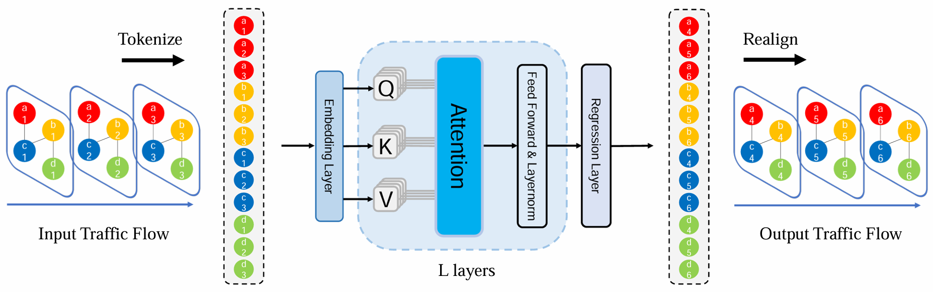
Figure 1: The Architecture of STformer and NSTformer

Pipeline

We present our pipeline and the architecture of our models in Figure 1. Without any complicated module or data process, we focus on how to capture the complex spatial-temporal relationships. Specifically, instead of regarding the traffic flow as a spatial-temporal graph, we just treat it as a regular 3D tensor and flatten it to a 1D sequence then feed to Transformer or its variant.

By this way, we can effectively capture the relationship between any pair of ST-Tokens. Correspondingly, the complexity of STformer is $O(N^{2}T^{2})$, which is unbearable when the input is too large. To overcome it, we desinged NSTformer with $O(NT)$ complexity, yielding a powerful and efficient model. And the only one difference between NSTformer and STformer is the attention mechanism, where the former with the linear Nyström attention while the latter with the quadratic self-attention.

Embedding Layer & Regression Layer

As the Figure 1 shows, our models are so concise that it just contains the embedding layers, attention mechanism and regression layers. And the only difference between STformer and NSTformer is their attention mechanism. We first introduce their common module, embedding layers and regression layers and present the models in detail later.

We follow (Liu et al. 2023) to set our embedding layers, in which they proposed a spatial-temporal adaptive embedding $E_{a}$ to capture the intricate spatial-temporal dependency rather than using any graph embedding.

Given the traffic flow $\textit{{X}}\in\mathbb{R}^{T\times N\times D}$, where $T$ is the length of the input time-steps and $N$ represents the number of sensors of road networks, the mainstream setting of the feature dimension $D$ is 3 which contains the value of traffic conditions such as speed, the time flag day-of-week from 1 to 7, the time flag timestamps-of-day from 1 to 288. We embed the three features to $E_{f}\in{\mathbb{R}^{T\times N\times 3d_{f}}}$, where $d_{f}$ is the dimension of the feature embedding. And the simple yet effective $E_{a}\in\mathbb{R}^{T\times N\times d_{a}}$ to capture intricate spatial-temporal dependencies. After the above embedding, the traffic flow then be $\textit{{X}}\in\mathbb{R}^{T\times N\times d_{h}}$, where $d_{h}$ equals to $3d_{f}+d_{a}$, we will introduce our specific setting of the embedding dimensions in Experiment.

After the attention module in STformer and NSTformer, the traffic flow will be mapped to $\textit{{X'}}\in\mathbb{R}^{T\times N\times d_{h}}$. Finally, our fully-connected Regression Layer $FC$ yields the prediction $\textbf{{Y}}=FC(\textbf{{X'}})\in\mathbb{R}^{T^{\prime}\times N\times d}$, where $T^{\prime}$ is the length prediction and the $d$ is the dimension of prediction value, which equals to 1 in our traffic forecasting setting.

STformer

In this paper, we refer to the standard self-attention in Transformer as self-attention, the approximated self-attention in NSTformer as Nyström attention.

As Figure 1 shows, we regard each nodes (sensors) at different time-steps as an independent ST-Token, and all ST-Tokens from one traffic flow form a sequence whose length is $N\times T$ to feed to attention. Here we present the traffic flow as $\textit{{X}}\in\mathbb{R}^{NT\times d_{h}}$. We have

$$Q=\textbf{{X}}W_{Q},K=\textbf{{X}}W_{K},V=\textbf{{X}}W_{V}$$ (3)

where $W_{Q},W_{K},W_{V}\in\mathbb{R}^{d_{h}\times d_{h}}$.

Then the score of the self-attention is calculated as:

$$S=softmax(\frac{QK^{T}}{\sqrt{d_{h}}})\in\mathbb{R}^{NT\times NT}$$ (4)

The final output of the self-attention is:

$$SelfAttention(Q,K,V)=softmax(\frac{QK^{T}}{\sqrt{d_{h}}})V\in\mathbb{R}^{NT\times d_{h}}$$ (5)

The equation (4) reveals that STformer can capture the spatial-temporal dependencies simultaneously and dynamically learn the spatial-relationship of the global space, which overcome the problems of Spatial-Temporal Graph frame work.

In the other hand, due to the quadratic complexity in equal (4), the computational complexity of STformer is $O(N^{2}T^{2})$, which limits the performance even feasibility of STformer when the input is large.

NSTformer

To overcome the above new obstacle, we designed NSTformer, in which we adapted Nyströmformer to replace the standard Transformer in STformer, yields a linear Nyström attention. Consider the only one difference of the two models is the attention mechanism, we generally introduce Nyströmformer (Xiong et al. 2021) and analysis the linear Nyström attention here, we recommend (Xiong et al. 2021) to learn more.

The Nyström-like methods approximate a matrix by sampling columns from the matrix. (Xiong et al. 2021) adapted the method to approximate the calculation of the original softmax matrix $S$ in equal (4). The fundamental insight involves utilizing landmarks $\tilde{K}$ and $\tilde{Q}$ derived from key $K$ and query $Q$ to formulate an efficient Nyström approximation without accessing the entire $QK^{T}$. In cases where the count of landmarks, $m$, much smaller than the sequence length $n$, the Nyström approximation exhibits linear scalability concerning both memory and time with respect to the input sequence length.

Definition 4 (Xiong et al. 2021). Assume that the selected landmarks for inputs $Q=[q_{1};...;q_{n}]$ and $K=[k_{1};...;k_{n}]$ are $\{\tilde{q_{j}}\}_{j=1}^{m}$ and $\{\tilde{k_{j}}\}_{j=1}^{m}$ respectively. We denote the matrix form of the corresponding landmarks as

For $\{\tilde{q_{j}}\}_{j=1}^{m},\tilde{Q}=[\tilde{q_{1}};...;\tilde{q_{m}}]\in\mathbb{R}^{m\times d_{h}}$

For $\{\tilde{k_{j}}\}_{j=1}^{m},\tilde{K}=[\tilde{k_{1}};...;\tilde{k_{m}}]\in\mathbb{R}^{m\times d_{h}}$

Then the $m\times m$ matrix is given by $A_{S}$ = softmax$(\frac{\tilde{Q}\tilde{K}^{T}}{\sqrt{d_{h}}})$.

And the Nyström form of the softmax matrix, $S=softmax(\frac{QK^{T}}{\sqrt{d_{h}}})$ is approximated as

$\hat{S}$ = softmax$(\frac{Q\tilde{K}^{T}}{\sqrt{d_{h}}}){A_{S}}^{+}$softmax$(\frac{\tilde{Q}K^{T}}{\sqrt{d_{h}}})$,

where ${A_{S}}^{+}$ is a Moore-Penrose pseudoinverse of $A_{S}$.

Lemma 1 (Xiong et al. 2021). For $A_{S}\in\mathbb{R}^{m\times m}$, the sequence $\{{Z_{j}}\}_{j=0}^{j=\infty}$ generated by (Razavi et al. 2014),

$$Z_{j+1}=\frac{1}{4}Z_{j}(13I-A_{S}Z_{j}(15I-A_{S}Z_{j}(7I-A_{S}Z_{j})))$$ (6)

converges to the Moore-Penrose inverse ${A_{S}}^{+}$ in the third order with initial approximation $Z_{0}$ satisfying $||A_{S}{A_{S}}^{+}-A_{S}Z_{0}||<1$.

By $Z^{*}$ with (6) in Lemma 1 to approximate ${A_{S}}^{+}$, then the Nyström approximation of $S$ becomes

$\hat{S}$ = softmax$(\frac{Q\tilde{K}^{T}}{\sqrt{d_{h}}})Z^{*}$softmax$(\frac{\tilde{Q}K^{T}}{\sqrt{d_{h}}})$.

Finally, we derive the Nyström attention:

$\hat{S}V$ = softmax$(\frac{Q\tilde{K}^{T}}{\sqrt{d_{h}}})Z^{*}$softmax$(\frac{\tilde{Q}K^{T}}{\sqrt{d_{h}}})V$.

We present the pipeline for Nyström approximation of softmax matrix in self-attention in Algorithm 2.

Landmarks selection

(Zhang, Tsang, and Kwok 2008; Vyas, Katharopoulos, and Fleuret 2020) used K-Means to select landmark points (Lee et al. 2019). Consider the EM-style updates in K-means is less preferable when using mini-batch training. (Xiong et al. 2021) suggested using Segment-means, which is similar to the local average pooling approach previously utilized in NLP literature (Shen et al. 2018).

Particularly, for inputs $Q=[q_{1};...;q_{n}]$ and $K=[k_{1};...;k_{n}]$, $n$ queries are divided into $m$ segments. Assuming $n$ is divisible by $m$ for simplicity, as we can pad inputs to a length divisible by $m$, let $l=n/m$. Landmark points for $Q$ and $K$ are then calculated as demonstrated in (7). And the whole process only need a simple scan of inputs, which yields a complexity of $O(n)$.

$$\tilde{q_{j}}=\sum_{i=(j-1)\times l+1}^{(j-1)\times l+m}\frac{q_{i}}{m},\tilde{k_{j}}=\sum_{i=(j-1)\times l+1}^{(j-1)\times l+m}\frac{k_{i}}{m}$$ (7)

We revisit the landmarks selection for spatial-temporal forecasting. Our insight is that at the same time, the nodes from the same one neighborhood of the road network have similar traffic conditions.

The hypothesis is reasonable, as the traffic conditions in a localized area are influenced by similar factors such as road capacity, traffic signals or nearby events. For example, in the downtown area of a city, which typically serves as a hub for business and commercial activities, the traffic patterns during rush hours might be characterized by high congestion due to the influx of commuters. This congestion is likely to spread across multiple nodes within the same vicinity, affecting adjacent streets and intersections. Conversely, in residential neighborhoods, the traffic state may be different, with peak times coinciding with school drop-offs and pickups or evening commutes, but generally experiencing lighter traffic compared to commercial districts.

Based on the understanding of spatial-temporal data, we introduce a landmarks selection algorithm for using Nyström attention in spatial-temporal forecasting tasks, which named after Spatial-Temporal Cluster Sampling (STCS) algorithm. Specifically, the whole nodes of road network are divided into clusters $c_{1}$ to $c_{s}$ according their distance, and during the $T$ time-steps, each cluster is regarded as a block which we term it ST-block. One can select suitable clustering algorithm to the datasets as long as it can cluster the nodes according their spatial relationships, in our experiment we use the Agglomerative Clustering from scikit-learn (scikit-learn developers 2024). As the above hypothesis, we assume the traffic condition of nodes from the same block follows a same Normal distribution. Then, one can sample a certain number of times to get the average value. Finally, $s\times T$ landmarks are selected, as presented in Algorithm 1 taking the example of computation of $\tilde{Q}$, that of $\tilde{K}$ has the same process. In this way, we add our insight for spatial-temporal data to landmarks selection. Note that the clustering operation can be finished before the landmarks selection once the road network is given, then we can immediately figure out that the procession of STCS also only require a simple scan for inputs as Segment-means, with $O(n)$ complexity.

Algorithm 1 Spatial-Temporal Cluster Sampling

Input: Query $Q$
Parameter: Time steps $T$, sampling iterations $p$, Clusters $c_{1},c_{2},...,c_{s}$.
Output: $\tilde{Q}$

1:  Let $\tilde{Q}=[\ \ ]$.

2:  for $t\leftarrow 1$ to $T$ do

3:     for $c\leftarrow c_{1}$ to $c_{s}$ do

4:        Compute the mean $\mu$ and the standard variation $\sigma$ of the cluster $c$.

5:        Let $Sum=0$.

6:        for $i\leftarrow 1$ to $p$ do

7:           Draw one sample $X\sim\mathcal{N}(\mu,\,\sigma^{2})$.

8:           $Sum=Sum+X$.

9:        end for

10:        $Sum=\frac{Sum}{p}$.

11:        Append $Sum$ to $\tilde{Q}$.

12:     end for

13:  end for

14:  return $\tilde{Q}=[\tilde{q_{1}};...;\tilde{q_{m}}]$, where $m=s\times T$.

Complexity analysis

We follow (Xiong et al. 2021) to analyze the complexity of Nyström attention, namely $\hat{S}V$.

The time complexity breakdown is as follows:

• Landmark selection using Segment-means takes $O(n)$.

• Iterative approximation of the pseudoinverse takes $O(m^{3})$ in the worse case.

• Matrix multiplication softmax$(\frac{Q\tilde{K}^{T}}{\sqrt{d_{h}}})\times Z^{*}$, softmax$(\frac{\tilde{Q}K^{T}}{\sqrt{d_{h}}})\times V$, (softmax$(\frac{Q\tilde{K}^{T}}{\sqrt{d_{h}}})\times Z^{*}$) $\times$ (softmax$(\frac{\tilde{Q}K^{T}}{\sqrt{d_{h}}})\times V$) take $O(nm^{2}+mnd_{h}+m^{3}+nmd_{h})$.

Then we have the overall time complexity $O(n+m^{3}+nm^{2}+mnd_{h}+m^{3}+nmd_{h})$.

The memory complexity breakdown is as follows:

• Storing landmarks matrix $\tilde{Q}$ and $\tilde{K}$ takes $O(md_{h})$.

• Storing four Nyström approximation matrices takes $O(nm+m^{2}+mn+nd_{h})$.

Then we have the overall memory complexity $O(md_{h}+nm+m^{2}+mn+nd_{h})$.

Obviously, when $m\ll n$, the time and memory complexity of Nyström attention are $O(n)$.

Correspondingly, the computational complexity of NSTformer is $O(NT)$.

Algorithm 2 Pipeline for Nyström approximation of softmax matrix in self-attention (Xiong et al. 2021)

Input: Query $Q$ and Key $K$.
Output: Nyström approximation of softmax matrix.

1:  Compute landmarks from input $Q$ and landmarks from input $K$, $\tilde{Q}$ and $\tilde{K}$ as the matrix form.

2:  Compute $\tilde{F}=$ softmax$(\frac{Q\tilde{K}^{T}}{\sqrt{d_{h}}})$, $\tilde{B}=$ softmax$(\frac{\tilde{Q}K^{T}}{\sqrt{d_{h}}})$.

3:  Compute $\tilde{A}=$ softmax$(\frac{\tilde{Q}\tilde{K}^{T}}{\sqrt{d_{h}}})^{+}$.

4:  return $\tilde{F}\times\tilde{A}\times\tilde{B}$.

Experiment

Table 1: Experimental Results on METR-LA and PEMS-BAY.

Datasets	Models	Horizon 3 (15 mins)			Horizon 6 (30 mins)			Horizon 12 (60 mins)
		MAE	RMSE	MAPE	MAE	RMSE	MAPE	MAE	RMSE	MAPE
METR-LA	HA	4.79	10.00	11.70%	5.47	11.45	13.50%	6.99	13.89	17.54%
	HI	6.80	14.21	16.72%	6.80	14.21	16.72%	6.80	14.20	10.15%
	VAR	4.42	7.80	13.00%	5.41	9.13	12.70%	6.52	10.11	15.80%
	SVR	3.39	8.45	9.30%	5.05	10.87	12.10%	6.72	13.76	16.70%
	FC-LSTM	3.44	6.30	9.60%	3.77	7.23	10.09%	4.37	8.69	14.00%
	DCRNN	2.77	5.38	7.30%	3.15	6.45	8.80%	3.60	7.60	10.50%
	AGCRN	2.85	5.53	7.63%	3.20	6.52	9.00%	3.59	7.45	10.47%
	STGCN	2.88	5.74	7.62%	3.47	7.24	9.57%	4.59	9.40	12.70%
	STSGCN	3.31	7.62	8.06%	4.13	9.77	10.29%	5.06	11.66	12.91%
	GWNet	2.69	5.15	6.90%	3.07	6.22	8.37%	3.53	7.37	10.01%
	MTGNN	2.69	5.18	6.88%	3.05	6.17	8.19%	3.49	7.23	9.87%
	GTS	2.75	5.27	7.21%	3.14	6.33	8.62%	3.59	7.44	10.25%
	ASTGCN	4.86	9.27	9.21%	5.43	10.61	10.13%	6.51	12.52	11.64%
	GMAN	2.80	5.55	7.41%	3.12	6.49	8.73%	3.44	7.35	10.07%
	STID	2.82	5.53	7.75%	3.19	6.57	9.39%	3.55	7.55	10.95%
	STNorm	2.81	5.57	7.40%	3.18	6.59	8.47%	3.57	7.51	10.24%
	PDFormer	2.83	5.45	7.77%	3.20	6.46	9.19%	3.62	7.47	10.91%
	STAEformer	2.65	5.11∗	6.85%	2.97∗	6.00∗	8.13%	3.34	7.02∗	9.70%
	ST-Mamba	2.64∗	5.17	6.61%∗	3.00	6.18	8.06%∗	3.33∗	7.10	9.56%∗
	STformer	2.60	4.90	6.75%	2.84	5.59	7.75%	3.12	6.45	8.93%
	NSTformer	2.58	4.87	6.69%	2.82	5.55	7.64%	3.09	6.39	8.78%
PEMS-BAY	HA	1.89	4.30	4.16%	2.50	5.82	5.62%	3.31	7.54	7.65%
	HI	3.06	7.05	6.85%	3.06	7.04	6.84%	3.05	7.03	6.83%
	VAR	1.74	3.16	3.60%	2.32	4.25	5.00%	2.93	5.44	6.50%
	SVR	1.85	3.59	3.80%	2.48	5.18	5.50%	3.28	7.08	8.00%
	FC-LSTM	2.05	4.19	4.80%	2.20	4.55	5.20%	2.37	4.96	5.70%
	DCRNN	1.38	2.95	2.90%	1.74	3.97	3.90%	2.07	4.74	4.90%
	AGCRN	1.35	2.88	2.91%	1.67	3.82	3.81%	1.94	4.50	4.55%
	STGCN	1.36	2.96	2.90%	1.81	4.27	4.17%	2.49	5.69	5.79%
	STSGCN	1.44	3.01	3.04%	1.83	4.18	4.17%	2.26	5.21	5.40%
	GWNet	1.30	2.74	2.73%	1.63	3.70	3.67%	1.95	4.52	4.63%
	MTGNN	1.32	2.79	2.77%	1.65	3.74	3.69%	1.94	4.49	4.53%
	GTS	1.34	2.83	2.82%	1.66	3.78	3.77%	1.95	4.43	4.58%
	ASTGCN	1.52	3.13	3.22%	2.01	4.27	4.48%	2.61	5.42	6.00%
	GMAN	1.34	2.91	2.86%	1.63	3.76	3.68%	1.86∗	4.32∗	4.37%∗
	STID	1.31	2.79	2.78%	1.64	3.73	3.73%	1.91	4.42	4.55%
	STNorm	1.33	2.82	2.76%∗	1.65	3.77	3.66%	1.92	4.45	4.46%
	PDFormer	1.32	2.83	2.78%	1.64	3.79	3.71%	1.91	4.43	4.51%
	STAEformer	1.31	2.78∗	2.76%∗	1.62	3.68	3.62%	1.88	4.34	4.41%
	ST-Mamba	1.30∗	2.89	2.94%	1.61∗	3.32∗	3.56%∗	1.88	4.38	4.40%
	STformer	1.14	2.32	2.34%	1.37	2.92	2.94%	1.60	3.64	3.61%
	NSTformer	1.14	2.31	2.33%	1.36	2.91	2.92%	1.60	3.64	3.59%

Datasets

METR-LA and PEMS-BAY are the two most commonly used datasets in traffic forecasting (Li et al. 2018), we select these and give a brief introduction of the two datasets in Table 2.

Experimental Setup

In our experiments, METR-LA and PEMS-BAY datasets are partitioned into training, validation, and test sets with a ratio of 7:1:2.

Following (Liu et al. 2023), in our models, the embedding dimension $d_{f}$ is 24, while $d_{a}$ is set to 80. The number of Tranformer layers in STformer and its invariant in NSTformer are 3, all models with 4 heads. Both input and forecasting length are configured to be 1 hour, namely 12 time-steps. As for the landmarks, (Xiong et al. 2021) states that 64 landmarks is sufficient to yield a robust approximation. In order to cluster all the nodes at each of the 12 time-steps, we set the number of landmarks to 72, namely, cluster the nodes to 6 neighborhoods. For cluster algorithm, we use Agglomerative Clustering from scikit-learn (scikit-learn developers 2024).

We select Adam as optimizer, set learning rate to 0.001 and weight decay to 0.0003, train 30 epochs to optimize masked mae loss. We use the mostly used three metrics, MAE (Mean Absolute Error), RMSE (Root Mean Squared Error), and MAPE (Mean Absolute Percentage Error) to evaluating forecasting performance.

All experiments were conducted on a server with Ubuntu 18.04.1 and NVIDIA A100 GPU with 320 GB memory in total. We use Python 3.9.13, Pytorch 1.13.0 and BasicTS (Shao et al. 2023) platform to run our models.

Table 2: Intro of Datasets

Datasets	Nodes	Steps	Freq	Range
METR-LA	207	34,272	5 mins	03-06/2012
PEMS-BAY	325	52,116	5 mins	01-05/2017

Baselines

We selected abundant and diverse baselines, HA (Historical Average), HI (Cui, Xie, and Zheng 2021), SVR (Smola and Schölkopf 2004) and VAR (Lu et al. 2016) are traditional forecasting methods. FC-LSTM (Sutskever, Vinyals, and Le 2014) is a typical deep learning method. DCRNN (Li et al. 2018), AGCRN (Bai et al. 2020), GTS (Shang and Chen 2021), GWNet (Wu et al. 2019), MTGNN (Wu et al. 2020b), STGCN (Yu, Yin, and Zhu 2018) and STSGCN (Song et al. 2020) are typical representative within the Spatial-Temporal Graph framework. Though with attention mechanism, ASTGCN (Guo et al. 2019), GMAN (Zheng et al. 2020), STID (Shao et al. 2022a), STNorm (Deng et al. 2021), PDFormer (Jiang et al. 2023) are still within the framework. STAEformer (Liu et al. 2023) used vanilla Transformer with proposed spatio-temporal adaptive embedding earned excellent performance in traffic forecasting task, but captured the spatial-temporal representation separately. Actually, the comparision between STAEformer and STformer can be regarded as an ablation study. We have noticed that ST-Mamba (Shao et al. 2024) introduced Mamba (Gu and Dao 2024) to traffic forecasting with a linear model complexity, we select it to give a pivotal comparison between linear attention and Mamba in spatial-temporal forecasting task.

Results Analysis

Table 1 shows our results. If STformer and NSTformer exceed all other models, we marked the results of STformer and NSTformer with underline and bold format respectively. In all cases, bold results are the best while results with asterisk represents the best model except STformer and NSTformer.

As it shows, NSTformer and STformer achieve best performance and second best performance respectively on almost all metrics. At the first glance, it could be astonishing that NSTformer can be a bit better than STformer. In a few cases, (Xiong et al. 2021) also discovered that Nyström attention is even slightly better than self-attention in NLP tasks. Based on the discovery, we propose an open problem here: Does approximate attention have any additional positive effect such as regularization ?

STAEformer and ST-Mamba are only inferior to NSTformer and STformer. Our work with with STAEformer reveal the power of pure attention in spatial-temporal forecasting. Due to learning the spatial and temporal relationships separately and asynchronously, our models exceed it with a big advantage. Though ST-Mamba also has linear complexity, it lags far behind our models.

Model Complexity

Table 3: Model Complexity on METR-LA

Models	Asymp	Params	Layers
STAEformer	$O(N^{2}+T^{2})$	3,004,264	6
STformer	$O(N^{2}T^{2})$	743,388	3
NSTformer	$O(NT)$	742,020	3

We present the complexity of STformer and NSTformer in Table 3, with the comparison to STAEformer, the parameters are recorded on METR-LA. STformer and NSTformer can capture spatial-temporal relationship between nodes with fewer layers thanks to the fully-connected setting, which yields fewer model parameters, indicating their afford cost further.

Conclusion

We investigated only using attention mechanism in spatial-temporal forecasting tasks to address the problems of existing works. Our STformer earn state-of-the-art performance with a large advantage. Given the quadratic complexity of Transformer and based on our insight to the instinct of spatial-temporal data, we propose NSTformer with linear complexity by adapting Nyströmformer to overcome the obstacle, which slightly exceed STformer surprisingly. Thanks to the leading performance and economical cost of NSTformer, we hope our work can offer insight to spatial-temporal forecasting. For future research, one can extend our method to more other spatial-temporal tasks. Another interesting direction is to try other linear attention or Mamba further. As for the cases where approximate attention beat standard self-attention slightly, we get a hypothesis after speculating the discovery : Approximate attention could have additional positive effect such as regularization. We propose the theoretically and practically meaningful open problem to machine learning community.

References

- Bai et al. (2020) Bai, L.; Yao, L.; Li, C.; Wang, X.; and Wang, C. 2020. Adaptive graph convolutional recurrent network for traffic forecasting. Advances in neural information processing systems, 33: 17804–17815.
- Beltagy, Peters, and Cohan (2020) Beltagy, I.; Peters, M. E.; and Cohan, A. 2020. Longformer: The long-document transformer. arXiv preprint arXiv:2004.05150.
- Cai et al. (2020) Cai, L.; Janowicz, K.; Mai, G.; Yan, B.; and Zhu, R. 2020. Traffic transformer: Capturing the continuity and periodicity of time series for traffic forecasting. Transactions in GIS, 24(3): 736–755.
- Chen et al. (2020) Chen, D.; Lin, Y.; Li, W.; Li, P.; Zhou, J.; and Sun, X. 2020. Measuring and relieving the over-smoothing problem for graph neural networks from the topological view. In Proceedings of the AAAI conference on artificial intelligence, volume 34, 3438–3445.
- Chen, O’Bray, and Borgwardt (2022) Chen, D.; O’Bray, L.; and Borgwardt, K. 2022. Structure-aware transformer for graph representation learning. In International Conference on Machine Learning, 3469–3489. PMLR.
- Chen et al. (2021a) Chen, L.; Lu, K.; Rajeswaran, A.; Lee, K.; Grover, A.; Laskin, M.; Abbeel, P.; Srinivas, A.; and Mordatch, I. 2021a. Decision transformer: Reinforcement learning via sequence modeling. Advances in neural information processing systems, 34: 15084–15097.
- Chen et al. (2021b) Chen, Y.; Zeng, Q.; Ji, H.; and Yang, Y. 2021b. Skyformer: Remodel self-attention with gaussian kernel and nystr” om method. Advances in Neural Information Processing Systems, 34: 2122–2135.
- Choromanski et al. (2020) Choromanski, K. M.; Likhosherstov, V.; Dohan, D.; Song, X.; Gane, A.; Sarlos, T.; Hawkins, P.; Davis, J. Q.; Mohiuddin, A.; Kaiser, L.; et al. 2020. Rethinking Attention with Performers. In International Conference on Learning Representations.
- Cui, Xie, and Zheng (2021) Cui, Y.; Xie, J.; and Zheng, K. 2021. Historical inertia: A neglected but powerful baseline for long sequence time-series forecasting. In Proceedings of the 30th ACM international conference on information & knowledge management, 2965–2969.
- Deng et al. (2021) Deng, J.; Chen, X.; Jiang, R.; Song, X.; and Tsang, I. W. 2021. St-norm: Spatial and temporal normalization for multi-variate time series forecasting. In Proceedings of the 27th ACM SIGKDD conference on knowledge discovery & data mining, 269–278.
- Deshpande et al. (2006) Deshpande, A.; Rademacher, L.; Vempala, S. S.; and Wang, G. 2006. Matrix approximation and projective clustering via volume sampling. Theory of Computing, 2(1): 225–247.
- Devlin et al. (2018) Devlin, J.; Chang, M.-W.; Lee, K.; and Toutanova, K. 2018. Bert: Pre-training of deep bidirectional transformers for language understanding. arXiv preprint arXiv:1810.04805.
- Dosovitskiy et al. (2020) Dosovitskiy, A.; Beyer, L.; Kolesnikov, A.; Weissenborn, D.; Zhai, X.; Unterthiner, T.; Dehghani, M.; Minderer, M.; Heigold, G.; Gelly, S.; et al. 2020. An image is worth 16x16 words: Transformers for image recognition at scale. arXiv preprint arXiv:2010.11929.
- Farahat, Ghodsi, and Kamel (2011) Farahat, A.; Ghodsi, A.; and Kamel, M. 2011. A novel greedy algorithm for Nyström approximation. In Proceedings of the Fourteenth International Conference on Artificial Intelligence and Statistics, 269–277. JMLR Workshop and Conference Proceedings.
- Feng et al. (2022) Feng, J.; Chen, Y.; Li, F.; Sarkar, A.; and Zhang, M. 2022. How powerful are k-hop message passing graph neural networks. Advances in Neural Information Processing Systems, 35: 4776–4790.
- Frieze, Kannan, and Vempala (2004) Frieze, A.; Kannan, R.; and Vempala, S. 2004. Fast Monte-Carlo algorithms for finding low-rank approximations. Journal of the ACM (JACM), 51(6): 1025–1041.
- Gittens and Mahoney (2016) Gittens, A.; and Mahoney, M. W. 2016. Revisiting the Nyström method for improved large-scale machine learning. The Journal of Machine Learning Research, 17(1): 3977–4041.
- Gu and Dao (2024) Gu, A.; and Dao, T. 2024. Mamba: Linear-Time Sequence Modeling with Selective State Spaces. arXiv:2312.00752.
- Guo et al. (2019) Guo, S.; Lin, Y.; Feng, N.; Song, C.; and Wan, H. 2019. Attention based spatial-temporal graph convolutional networks for traffic flow forecasting. In Proceedings of the AAAI conference on artificial intelligence, volume 33, 922–929.
- Han et al. (2021) Han, L.; Du, B.; Sun, L.; Fu, Y.; Lv, Y.; and Xiong, H. 2021. Dynamic and multi-faceted spatio-temporal deep learning for traffic speed forecasting. In Proceedings of the 27th ACM SIGKDD conference on knowledge discovery & data mining, 547–555.
- He et al. (2016) He, K.; Zhang, X.; Ren, S.; and Sun, J. 2016. Deep residual learning for image recognition. In Proceedings of the IEEE conference on computer vision and pattern recognition, 770–778.
- Jiang et al. (2023) Jiang, J.; Han, C.; Zhao, W. X.; and Wang, J. 2023. PDFormer: Propagation Delay-aware Dynamic Long-range Transformer for Traffic Flow Prediction. In AAAI. AAAI Press.
- Katharopoulos et al. (2020) Katharopoulos, A.; Vyas, A.; Pappas, N.; and Fleuret, F. 2020. Transformers are rnns: Fast autoregressive transformers with linear attention. In International conference on machine learning, 5156–5165. PMLR.
- Keles, Wijewardena, and Hegde (2023) Keles, F. D.; Wijewardena, P. M.; and Hegde, C. 2023. On the computational complexity of self-attention. In International Conference on Algorithmic Learning Theory, 597–619. PMLR.
- Kidger and Lyons (2020) Kidger, P.; and Lyons, T. 2020. Universal approximation with deep narrow networks. In Conference on learning theory, 2306–2327. PMLR.
- Kim et al. (2022) Kim, J.; Nguyen, D.; Min, S.; Cho, S.; Lee, M.; Lee, H.; and Hong, S. 2022. Pure transformers are powerful graph learners. Advances in Neural Information Processing Systems, 35: 14582–14595.
- Kipf and Welling (2016) Kipf, T. N.; and Welling, M. 2016. Semi-Supervised Classification with Graph Convolutional Networks. In International Conference on Learning Representations.
- Kitaev, Kaiser, and Levskaya (2019) Kitaev, N.; Kaiser, L.; and Levskaya, A. 2019. Reformer: The Efficient Transformer. In International Conference on Learning Representations.
- Kumar, Mohri, and Talwalkar (2009) Kumar, S.; Mohri, M.; and Talwalkar, A. 2009. Ensemble nystrom method. Advances in Neural Information Processing Systems, 22.
- Kumar, Mohri, and Talwalkar (2012) Kumar, S.; Mohri, M.; and Talwalkar, A. 2012. Sampling methods for the Nyström method. The Journal of Machine Learning Research, 13(1): 981–1006.
- Lee et al. (2019) Lee, J.; Lee, Y.; Kim, J.; Kosiorek, A.; Choi, S.; and Teh, Y. W. 2019. Set Transformer: A Framework for Attention-based Permutation-Invariant Neural Networks. In Chaudhuri, K.; and Salakhutdinov, R., eds., Proceedings of the 36th International Conference on Machine Learning, volume 97 of Proceedings of Machine Learning Research, 3744–3753. PMLR.
- Li, Kwok, and Lü (2010) Li, M.; Kwok, J. T.-Y.; and Lü, B. 2010. Making large-scale Nyström approximation possible. In Proceedings of the 27th International Conference on Machine Learning, ICML 2010, 631.
- Li et al. (2019) Li, S.; Jin, X.; Xuan, Y.; Zhou, X.; Chen, W.; Wang, Y.-X.; and Yan, X. 2019. Enhancing the locality and breaking the memory bottleneck of transformer on time series forecasting. Advances in neural information processing systems, 32.
- Li et al. (2018) Li, Y.; Yu, R.; Shahabi, C.; and Liu, Y. 2018. Diffusion Convolutional Recurrent Neural Network: Data-Driven Traffic Forecasting. In International Conference on Learning Representations.
- Likhosherstov et al. (2021) Likhosherstov, V.; Choromanski, K. M.; Davis, J. Q.; Song, X.; and Weller, A. 2021. Sub-linear memory: How to make performers slim. Advances in Neural Information Processing Systems, 34: 6707–6719.
- Lin et al. (2023) Lin, J.; Li, Z.; Li, Z.; Bai, L.; Zhao, R.; and Zhang, C. 2023. Dynamic causal graph convolutional network for traffic prediction. arXiv preprint arXiv:2306.07019.
- Liu et al. (2023) Liu, H.; Dong, Z.; Jiang, R.; Deng, J.; Deng, J.; Chen, Q.; and Song, X. 2023. Spatio-temporal adaptive embedding makes vanilla transformer sota for traffic forecasting. In Proceedings of the 32nd ACM International Conference on Information and Knowledge Management, 4125–4129.
- Liu et al. (2021) Liu, Z.; Lin, Y.; Cao, Y.; Hu, H.; Wei, Y.; Zhang, Z.; Lin, S.; and Guo, B. 2021. Swin transformer: Hierarchical vision transformer using shifted windows. In Proceedings of the IEEE/CVF international conference on computer vision, 10012–10022.
- Livni, Shalev-Shwartz, and Shamir (2014) Livni, R.; Shalev-Shwartz, S.; and Shamir, O. 2014. On the computational efficiency of training neural networks. Advances in neural information processing systems, 27.
- Lu et al. (2021) Lu, J.; Yao, J.; Zhang, J.; Zhu, X.; Xu, H.; Gao, W.; Xu, C.; Xiang, T.; and Zhang, L. 2021. Soft: Softmax-free transformer with linear complexity. Advances in Neural Information Processing Systems, 34: 21297–21309.
- Lu and Lu (2020) Lu, Y.; and Lu, J. 2020. A universal approximation theorem of deep neural networks for expressing probability distributions. Advances in neural information processing systems, 33: 3094–3105.
- Lu et al. (2016) Lu, Z.; Zhou, C.; Wu, J.; Jiang, H.; and Cui, S. 2016. Integrating Granger Causality and Vector Auto-Regression for Traffic Prediction of Large-Scale WLANs. KSII Transactions on Internet & Information Systems, 10(1).
- Peng et al. (2021) Peng, H.; Pappas, N.; Yogatama, D.; Schwartz, R.; Smith, N.; and Kong, L. 2021. Random Feature Attention. In International Conference on Learning Representations (ICLR 2021).
- Razavi et al. (2014) Razavi, M. K.; Kerayechian, A.; Gachpazan, M.; and Shateyi, S. 2014. A New Iterative Method for Finding Approximate Inverses of Complex Matrices. In Abstract and Applied Analysis, volume 2014, 1–7. Hindawi.
- Roy et al. (2021) Roy, A.; Saffar, M.; Vaswani, A.; and Grangier, D. 2021. Efficient content-based sparse attention with routing transformers. Transactions of the Association for Computational Linguistics, 9: 53–68.
- scikit-learn developers (2024) scikit-learn developers. 2024. Agglomerative Clustering. https://scikit-learn.org/stable/modules/generated/sklearn.cluster.AgglomerativeClustering.html. Accessed: 2024-08-16.
- Shang and Chen (2021) Shang, C.; and Chen, J. 2021. Discrete Graph Structure Learning for Forecasting Multiple Time Series. In Proceedings of International Conference on Learning Representations.
- Shao et al. (2024) Shao, Z.; Bell, M. G. H.; Wang, Z.; Geers, D. G.; Xi, H.; and Gao, J. 2024. ST-Mamba: Spatial-Temporal Selective State Space Model for Traffic Flow Prediction. arXiv:2404.13257.
- Shao et al. (2023) Shao, Z.; Wang, F.; Xu, Y.; Wei, W.; Yu, C.; Zhang, Z.; Yao, D.; Jin, G.; Cao, X.; Cong, G.; Jensen, C. S.; and Cheng, X. 2023. Exploring Progress in Multivariate Time Series Forecasting: Comprehensive Benchmarking and Heterogeneity Analysis. arXiv:2310.06119.
- Shao et al. (2022a) Shao, Z.; Zhang, Z.; Wang, F.; Wei, W.; and Xu, Y. 2022a. Spatial-temporal identity: A simple yet effective baseline for multivariate time series forecasting. In Proceedings of the 31st ACM International Conference on Information & Knowledge Management, 4454–4458.
- Shao et al. (2022b) Shao, Z.; Zhang, Z.; Wei, W.; Wang, F.; Xu, Y.; Cao, X.; and Jensen, C. S. 2022b. Decoupled dynamic spatial-temporal graph neural network for traffic forecasting. arXiv preprint arXiv:2206.09112.
- Shen et al. (2018) Shen, D.; Wang, G.; Wang, W.; Min, M. R.; Su, Q.; Zhang, Y.; Li, C.; Henao, R.; and Carin, L. 2018. Baseline Needs More Love: On Simple Word-Embedding-Based Models and Associated Pooling Mechanisms. In Gurevych, I.; and Miyao, Y., eds., Proceedings of the 56th Annual Meeting of the Association for Computational Linguistics (Volume 1: Long Papers), 440–450. Melbourne, Australia: Association for Computational Linguistics.
- Si, Hsieh, and Dhillon (2016) Si, S.; Hsieh, C.-J.; and Dhillon, I. 2016. Computationally efficient Nyström approximation using fast transforms. In International conference on machine learning, 2655–2663. PMLR.
- Smola and Schölkopf (2004) Smola, A. J.; and Schölkopf, B. 2004. A tutorial on support vector regression. Statistics and computing, 14: 199–222.
- Song et al. (2020) Song, C.; Lin, Y.; Guo, S.; and Wan, H. 2020. Spatial-temporal synchronous graph convolutional networks: A new framework for spatial-temporal network data forecasting. In Proceedings of the AAAI conference on artificial intelligence, volume 34, 914–921.
- Sutskever, Vinyals, and Le (2014) Sutskever, I.; Vinyals, O.; and Le, Q. V. 2014. Sequence to sequence learning with neural networks. Advances in neural information processing systems, 27.
- Valiant (1984) Valiant, L. G. 1984. A theory of the learnable. Communications of the ACM, 27(11): 1134–1142.
- Vaswani et al. (2017) Vaswani, A.; Shazeer, N.; Parmar, N.; Uszkoreit, J.; Jones, L.; Gomez, A. N.; Kaiser, L. u.; and Polosukhin, I. 2017. Attention is All you Need. In Guyon, I.; Luxburg, U. V.; Bengio, S.; Wallach, H.; Fergus, R.; Vishwanathan, S.; and Garnett, R., eds., Advances in Neural Information Processing Systems, volume 30. Curran Associates, Inc.
- Vyas, Katharopoulos, and Fleuret (2020) Vyas, A.; Katharopoulos, A.; and Fleuret, F. 2020. Fast Transformers with Clustered Attention. In Larochelle, H.; Ranzato, M.; Hadsell, R.; Balcan, M.; and Lin, H., eds., Advances in Neural Information Processing Systems, volume 33, 21665–21674. Curran Associates, Inc.
- Wang et al. (2023) Wang, J.; Jiang, J.; Jiang, W.; Han, C.; and Zhao, W. X. 2023. Towards Efficient and Comprehensive Urban Spatial-Temporal Prediction: A Unified Library and Performance Benchmark. arXiv preprint arXiv:2304.14343.
- Wang et al. (2020) Wang, S.; Li, B. Z.; Khabsa, M.; Fang, H.; and Ma, H. 2020. Linformer: Self-attention with linear complexity. arXiv preprint arXiv:2006.04768.
- Wu et al. (2020a) Wu, S.; Xiao, X.; Ding, Q.; Zhao, P.; Wei, Y.; and Huang, J. 2020a. Adversarial sparse transformer for time series forecasting. Advances in neural information processing systems, 33: 17105–17115.
- Wu et al. (2020b) Wu, Z.; Pan, S.; Long, G.; Jiang, J.; Chang, X.; and Zhang, C. 2020b. Connecting the dots: Multivariate time series forecasting with graph neural networks. In Proceedings of the 26th ACM SIGKDD international conference on knowledge discovery & data mining, 753–763.
- Wu et al. (2019) Wu, Z.; Pan, S.; Long, G.; Jiang, J.; and Zhang, C. 2019. Graph WaveNet for Deep Spatial-Temporal Graph Modeling. In Proceedings of the Twenty-Eighth International Joint Conference on Artificial Intelligence, IJCAI-19, 1907–1913. International Joint Conferences on Artificial Intelligence Organization.
- Xiong et al. (2021) Xiong, Y.; Zeng, Z.; Chakraborty, R.; Tan, M.; Fung, G.; Li, Y.; and Singh, V. 2021. Nyströmformer: A nyström-based algorithm for approximating self-attention. In Proceedings of the AAAI Conference on Artificial Intelligence, volume 35, 14138–14148.
- Xu et al. (2020) Xu, M.; Dai, W.; Liu, C.; Gao, X.; Lin, W.; Qi, G.-J.; and Xiong, H. 2020. Spatial-temporal transformer networks for traffic flow forecasting. arXiv preprint arXiv:2001.02908.
- Yu, Yin, and Zhu (2018) Yu, B.; Yin, H.; and Zhu, Z. 2018. Spatio-temporal graph convolutional networks: a deep learning framework for traffic forecasting. In Proceedings of the 27th International Joint Conference on Artificial Intelligence, 3634–3640.
- Yun et al. (2019) Yun, S.; Jeong, M.; Kim, R.; Kang, J.; and Kim, H. J. 2019. Graph transformer networks. Advances in neural information processing systems, 32.
- Zaheer et al. (2020) Zaheer, M.; Guruganesh, G.; Dubey, K. A.; Ainslie, J.; Alberti, C.; Ontanon, S.; Pham, P.; Ravula, A.; Wang, Q.; Yang, L.; et al. 2020. Big bird: Transformers for longer sequences. Advances in neural information processing systems, 33: 17283–17297.