On the KL-Divergence-based Robust Satisficing Model

Abstract

Empirical risk minimization, a cornerstone in machine learning, is often hindered by the Optimizer’s Curse stemming from discrepancies between the empirical and true data-generating distributions. To address this challenge, the robust satisficing framework has emerged recently to mitigate ambiguity in the true distribution. Distinguished by its interpretable hyperparameter and enhanced performance guarantees, this approach has attracted increasing attention from academia. However, its applicability in tackling general machine learning problems, notably deep neural networks, remains largely unexplored due to the computational challenges in solving this model efficiently across general loss functions. In this study, we delve into the Kullback–Leibler-divergence-based robust satisficing model under a general loss function, presenting analytical interpretations, diverse performance guarantees, efficient and stable numerical methods, convergence analysis, and an extension tailored for hierarchical data structures. Through extensive numerical experiments across three distinct machine learning tasks, we demonstrate the superior performance of our model compared to state-of-the-art benchmarks.

1 Introduction

Stochastic optimization models have been highly successful and extensively widely employed across a variety of domains of machine learning. A conventional approach for solving these models rely on the framework of Empirical Risk Minimization (ERM), which focuses on optimizing the expected performance over the empirical distribution derived from the training data. The performance of the ERM model is greatly influenced by the quality of the training data in accurately representing the true distribution. For example, models trained based on ERM may perform poorly under a shifted distribution, sometimes even worse than an untrained model [1; 11; 16; 41], because the training samples does not accurately reflect the testing distribution. Even the train samples and test samples are generated from the same distribution, the empirical optimization results tend to be optimistically biased, leading to unsatisfactory performance on unseen samples. This phenomenon is usually called the Optimizer’s Curse [63].

To enhance model robustness towards discrepancy between the training data and the true data-generating distribution, distributionally robust optimization (DRO) is proposed and adopted across a variety of domains [13; 69; 4; 45]. The foundation of DRO models features an ambiguity set of possible true distributions and optimizes the worst-case expected performance over this set. Accounting for various possible distribution shifts, the out-of-sample performance is guaranteed to be as strong as that of the DRO objective if the true distribution lies in the ambiguity set.

Recently, a novel framework, namely, Robust Satisficing (RS) is proposed to tackle the challenges of distribution shifts [43; 70]. Compared with DRO, RS protects the model beyond distribution shifts that are confined within an ambiguity set. Specifically, it aims to maintain an acceptable level of loss under a reference distribution and minimizes the fragility to impacts of distribution shifts on amplifying losses [61]. The impact of distribution shifts is typically characterized by a probability distance function (e.g. Wasserstein distance or Kullback-Leibler divergence) from the reference distribution. Existing research focuses on transforming the RS model with Wasserstein distance into a tractable mathematical programming form if the loss function exhibits linearity or concave-convex properties, applies it to specific problems in different fields[43; 70; 61]. Within the realm of general machine learning tasks, the Wasserstein distance is inadequate for addressing non-geometric perturbations and may be hindered by computational challenges in practice [49; 67]. Alternatively, the Kullback-Leibler (KL) divergence, a metric for quantifying the disparity in information between two distributions, is widely adopted in machine learning applications, such as label distribution shift [21; 72; 22], disentangled representation learning [34; 26], domain generalization [75; 48]. However, the performance of KL-divergence-based RS models has received limited investigation, with only one study addressing its application in binary classification [70], thereby its applicability in tackle general machine learning tasks, such as deep neural networks, remains unexplored.

In this paper, we establish a comprehensive analysis of the Kullback-Leibler Robust Satisficing (KL-RS) model, and provide necessary theoretical foundations. In addition, we explores the analytical interpretations behind this model, designs tailored solution algorithms, conducts thorough experiments, and extends its applicability for hierarchical data structures.

1.1 Contribution

Our main contribution can be summarized as follows:

(i). We introduce a novel KL-RS framework tailored for general machine learning tasks, which achieves the highest robustness given a tangible tolerance. In light of the hierarchical nature of data generation in prevailing applications, we present an adaptation of KL-RS named hierarchical KL-RS.

(ii). As a comprehensive investigation of the KL-RS model, we establish interesting analytical interpretations and novel performance guarantees. Moreover, we develop numerical algorithms for solving both KL-RS and hierarchical KL-RS model based on alternative optimization and explorations of the monotonicity and convex structure, and provide analysis of convergence guarantees. Notably, we identify two pivotal advantages of our algorithm: unbiasedness and normalization, to ensure the efficient and stable performance compared with existing approaches.

(iii). Finally, we conduct thorough numerical experiments across three distinct machine learning tasks (label distribution shift, long-tailed learning, fair PCA), and the (hierarchical) KL-RS model outperforms problem-specific state-of-the-art benchmarks and universal DRO benchmarks. Our results demonstrate the effectiveness and versatility of the (hierarchical) KL-RS model in practical machine learning applications. Additionally, we offer in-depth and visual analysis on how the tolerance and fragile measure can affect the performance under varying distribution shifts.

1.2 Related Work

Our paper centers on the development of the KL-RS model and establishes its wide applicability in machine learning tasks. Existing research on RS in related applications typically adopts the Wasserstein distance [61; 70], because Wasserstein distance is suitable for capturing geometric perturbations of distributions, showcased in works on adversarial examples [62; 23]. However, it fails to measure non-geometric distribution shift which is common in machine learning community, e.g., transitional kernel shift in MDP [57; 68], label distribution shift[72; 21; 22] and domain adaptation[76; 75]. As the computational challenges encountered by Wasserstein-distance-based models under general loss function in practical applications, existing work typically focus on exploring tractable reformulations through assuming the linearity or concave-convex properties of the loss function [43; 61; 70; 62].

KL divergence has received significant attention in machine learning community in addressing distribution shifts [75; 34; 26]. Nevertheless, the performance of KL-RS models remains under explored nowadays, with a solitary study examining its performance in binary classification [70], indicating a notable gap in systematic investigation of this framework. The effectiveness of the KL-RS model has been validated in operations management applications [77; 31; 24]. Most models are reformulated into conic optimization problems that can be solved via commercial solvers. These solution methods rely on the structure of the operations management applications and are not directly applicable to complex functions commonly seen in machine learning tasks, such as neural networks.

2 Preliminaries

Notation. We denote vectors in boldface lowercase letters. We use $\tilde{z}$ and $\tilde{\boldsymbol{z}}$ with a tilde sign to denote a random variable and a random vector, respectively. A probability distributions is denoted by $\mathbb{P}$, $\mathbb{P}\in\mathcal{P}(\Omega)$, where $\mathcal{P}(\Omega)$ represents the set of all Borel probability distributions on the support $\Omega\subseteq\mathbb{R}^{n}$. Moreover, $\mathbb{E}_{\mathbb{P}}[\tilde{z}]$ and $\mathbb{V}_{\mathbb{P}}[\tilde{z}]$ are the expectation and variance of a random variable, $\tilde{z}\sim\mathbb{P}$, over its distribution. Lastly, we use $[N]$ to denote the index set $\{1,2,...,N\}$.

Kullback–Leibler divergence. The Kullback–Leibler (KL) divergence, denoted as $D_{KL}(\mathbb{Q}\|\mathbb{P})$, is a measure of discrepancy of a probability distribution $\mathbb{Q}$ from a reference distribution $\mathbb{P}$ as defined below:

$$D_{KL}(\mathbb{Q}\|\mathbb{P})=\mathbb{E}_{\mathbb{Q}}\left[\log\left(\frac{d\mathbb{Q}}{d\mathbb{P}}\right)\right]\;\;\text{ if }\;\;\mathbb{Q}\ll\mathbb{P},$$ (1)

where we use $\mathbb{Q}\ll\mathbb{P}$ to denote that $\mathbb{Q}$ is absolutely continuous with respect to $\mathbb{P}$[65]. This non-symmetric measurement is closely related to concepts such as relative entropy, information divergence, and discrimination information.

Data-driven stochastic optimization. In the context of statistical learning, we want to minimize some prediction loss over all possible parameter values of the learning model. Let $\Theta$ denote the set of model parameters and measurable continuous function $l:\Theta\times\mathbb{R}^{n}\to\mathbb{R}$ denote the loss function. For any $\boldsymbol{\theta}\in\Theta$ and $\bm{z}\in\mathbb{R}^{n}$, $l(\boldsymbol{\theta},\bm{z})$ measures the prediction error of model $\boldsymbol{\theta}$ on a data realization $\bm{z}$. A stochastic optimization model typically solves the following problem:

$$\min_{\boldsymbol{\theta}\in\Theta}\mathbb{E}_{\mathbb{P}^{*}}[l(\boldsymbol{\theta},\tilde{\boldsymbol{z}})],$$ (2)

where $\mathbb{P}^{*}$ is the true data-generating distribution of $\tilde{\boldsymbol{z}}$.

In practice, we typically do not know the true distribution $\mathbb{P}^{*}$. A common approximation is to replace the true distribution with the empirical distribution constructed from a set of historical samples of size $N$, $\{\hat{\bm{z}}_{1},\ldots,\hat{\bm{z}}_{N}\}$. We use $\hat{\mathbb{P}}$ to represent the empirical distribution, i.e., $\hat{\mathbb{P}}(\tilde{\boldsymbol{z}}=\hat{\boldsymbol{z}}_{i})=1/N$. The empirical optimization problem is cast as follows:

$$E_{0}=\min_{\boldsymbol{\theta}\in\Theta}\mathbb{E}_{\hat{\mathbb{P}}}[l(\boldsymbol{\theta},\tilde{\boldsymbol{z}})]=\min_{\boldsymbol{\theta}\in\Theta}\frac{1}{N}\sum_{i=1}^{N}l(\boldsymbol{\theta},\hat{\boldsymbol{z}}_{i}).$$ (3)

The empirical optimization problem (3) is widely adopted in the field of machine learning. For instance, the Empirical Risk Minimization (ERM) framework falls within the scope of (3), defining a broad range of models and applications.

Distributionally robust approaches. When a stochastic program is calibrated based on one dataset but is evaluated on a separate dataset, the out-of-sample performance is frequently found to be unsatisfactory. This phenomenon is known as the optimizer’s curse [63]. Inherently, the empirical optimization may yield an inferior solution that performs poorly out-of-sample when the historical data is not sufficient [36; 60].

To account for the discrepancy between the empirical distribution and the true data-generating distribution, Data-driven Distributionally Robust Optimization (DRO) incorporates a probability-distance-based ambiguity set of potential distributions $\mathcal{B}(r)$, and solves

$$\min_{\boldsymbol{\theta}\in\Theta}\max_{\mathbb{P}\in\mathcal{B}(r)}\mathbb{E}_{\mathbb{P}}[l(\boldsymbol{\theta},\tilde{\boldsymbol{z}})]\quad\text{where}\;\;\mathcal{B}(r)\triangleq\{\mathbb{P}\in\mathcal{P}(\Omega):D(\mathbb{P}\|\hat{\mathbb{P}})\leq r\}.$$ (4)

Common choices of probability distance $D$ include Wasserstein metric, KL divergence, and generalized $\phi$-divergence [46; 20; 16; 14].

The classic DRO model hedges against $\mathbb{P}^{*}\in\mathcal{B}(r)$ but it leads to no guarantee when $\mathbb{P}^{*}$ is outside $\mathcal{B}(r)$. Recently, a novel development in optimization under uncertainty is the Robust Satisficing framework [43], which can provide performance guarantees under all possible only distributions rather than distributions in $\mathcal{B}(r)$. The robust satisficing model can be written as the following:

$$\min_{\lambda\geq 0,\boldsymbol{\theta}\in\Theta} \quad\lambda$$ (5)

s.t. $$\quad\mathbb{E}_{\mathbb{\mathbb{P}}}[l(\boldsymbol{\theta},\tilde{\boldsymbol{z}})]\leq\tau+\lambda D(\mathbb{\mathbb{P}}\|\hat{\mathbb{P}})\quad\forall\mathbb{P}\in\mathcal{P}(\Omega),$$

where $D$ represents a probability distance measure and $\tau$ denotes a prescribed threshold for the prediction loss. The optimal value $\lambda^{*}$ is called the fragility measure [43] or the fragility index [70], and it measures the robustness of the learning parameter $\boldsymbol{\theta}$.

3 KL Divergence based Robust Satisficing Model

3.1 Problem Formulation and Guarantees

We adopt the KL Divergence in the robust satisficing model (5), and formulate a KL-Divergence-based Robust Satisficing (KL-RS) Model as follows:

$$\min_{\lambda\geq 0,\boldsymbol{\theta}\in\Theta} \quad\lambda$$ (6)

s.t. $$\quad\mathbb{E}_{\mathbb{\mathbb{P}}}[l(\boldsymbol{\theta},\tilde{\boldsymbol{z}})]\leq\tau+\lambda D_{KL}(\mathbb{\mathbb{P}}\|\hat{\mathbb{P}})\quad\forall\mathbb{P}\in\{\mathbb{P}_{0}\in\mathcal{P}(\Omega):\mathbb{P}_{0}\ll\hat{\mathbb{P}}\}.$$

The decision variable $\lambda$ quantifies the maximally allowed magnitude of constraint violation caused by the discrepancy of the true distribution $\mathbb{P}^{*}$ from the empirical distribution $\hat{\mathbb{P}}$. Specifically, a small value of $\lambda$ suggests that only minor violations are expected even if the true distribution is significantly different from the empirical estimate.

According to the properties of the KL divergence, we can reformulate the KL-RS model (5).

Theorem 3.1.

The KL-RS model (6) is equivalent to

$$\min_{\lambda\geq 0,\boldsymbol{\theta}\in\Theta} \quad\lambda$$ (7)

s.t. $$\quad\hat{R}(\boldsymbol{\theta},\lambda)\leq\tau,$$

with $\hat{R}(\boldsymbol{\theta},\lambda)\triangleq\lambda\log\left(\mathbb{E}_{\hat{\mathbb{P}}}\left[\exp\left(l(\boldsymbol{\theta},\tilde{\boldsymbol{z}})/\lambda\right)\right]\right)$.

The term $\hat{R}(\boldsymbol{\theta},\lambda)$ is called $\frac{1}{\lambda}$-tilted loss in [39; 38; 54]. Instead of selecting $\lambda$ as a hyperparameter for tilted empirical risk minimization, the KL-RS model selects hyperparameter $\tau$, an acceptable loss of optimality relative to the empirical risk model (3), and obtains the highest robustness by optimizing $\lambda$. The benefits of the KL-RS model include a more tangible selection of tolerance $\tau$ [57] and enhanced numerical performance and stability, as demonstrated in Section 4 and Appendix B.

This simplified formulation in Theorem 3.1 enables us better understand the KL-RS problem (6). We demonstrate the analytical interpretations of the KL-RS model and performance guarantees. For the sake of concise and clarity, all proofs of theorems and propositions are relegated to Appendix E.

Analytical Interpretations. We offer analytical interpretations of the KL-RS model from dual perspectives. From a model formulation standpoint, we demonstrate its characterization as an empirical mean-variance constrained optimization paradigm, particularly when $\tau$ closely aligns with the empirical loss $\mathbb{E}_{\hat{\mathbb{P}}}[l(\boldsymbol{\theta},\tilde{\boldsymbol{z}})]$. Concerning optimal distribution, the KL-RS model enhances the influence of samples with large losses to bolster its robustness. Detailed discussions and propositions are provided in the Appendix A.

Tail probability guarantee. Beyond analytical interpretation, we present a tail probability guarantee of the KL-RS model.

Proposition 3.2.

Given a non-negative number $\alpha$, we have

$$\hat{\mathbb{P}}(l(\boldsymbol{\theta},\tilde{\boldsymbol{z}})\geq\tau+\alpha)\leq\exp(-\alpha/\lambda)$$

for every feasible solution $(\boldsymbol{\theta},\lambda)$ of the KL-RS model.

From Proposition 3.2, we can see that the probability of exceeding the tolerance $\tau$ decays exponentially. Moreover, the optimal $\lambda_{N}^{*}$ attained by the KL-RS model yields the most favorable exponential rate, as $\exp(-\alpha/\lambda)$ is decreasing in $\lambda$, consistent with the observation in previous literature [77; 70].

Asymptotic performance guarantee. Note that if $\mathbb{P}^{*}$ is a discrete distribution supported by $K$ points, then $2N\cdot D_{KL}(\mathbb{P}^{*}\|\hat{\mathbb{P}})\to\chi^{2}_{K-1}$ as $N\to\infty$ [51]. Based on this property of asymptotic convergence, we establish the following theorem.

Theorem 3.3.

Suppose that $\mathbb{P}^{*}$ is a discrete distribution supported by $k$ points. For optimal solution $(\boldsymbol{\theta}^{*}_{N},\lambda^{*}_{N})$ of the KL-RS model and a given non-negative radius $r\geq 0$, we have

$$\mathbb{P}^{N}\left(\mathbb{E}_{\mathbb{P}^{*}}[l(\boldsymbol{\theta}^{*}_{N},\tilde{\boldsymbol{z}}))<\tau+\lambda^{*}_{N}r\right)\geq\chi^{2}_{K-1}(\tilde{y}\leq 2Nr)\quad\text{as }\;N\to\infty,$$ (8)

where we use $\mathbb{P}^{N}$ to denote the distribution that governs the distribution of independent samples $\{\hat{\boldsymbol{z}}_{i}\}_{i\in[N]}$ drawn from $\mathbb{P}^{*}$, and $\tilde{y}\sim\chi^{2}_{K-1}$ is a chi-squared distribution with degree of freedom $K-1$.

Intuitively, this asymptotic result suggests that the optimal decision $(\boldsymbol{\theta}^{*}_{N},\lambda^{*}_{N})$ of the KL-RS model with $N$ samples enjoys a high confidence that the expected loss under the true distribution would not exceed the threshold $\tau$ by $\lambda^{*}_{N}r$. In addition, as $\chi^{2}_{K-1}(\tilde{y}\leq 2Nr)\geq 1-\left(m\cdot\exp(1-m)\right)^{(K-1)/2}$ with $m=2Nr/(K-1)$ by the Chernoff inequality, we can estimate the required sample size for a desired precision.

Theorem 3.4.

Suppose that $\mathbb{P}^{*}$ is a continuous distribution and a constant $C$ such that $|l(\boldsymbol{\theta},\tilde{\boldsymbol{z}})|\leq C$ exists. For every feasible solution $(\boldsymbol{\theta}^{*}_{N},\lambda^{*}_{N})$ of the KL-RS model and a given non-negative radius $r\geq 0$, we have

$$\mathbb{P}^{N}\left(\mathbb{E}_{\mathbb{P}^{*}}[l(\boldsymbol{\theta}^{*}_{N},\tilde{\boldsymbol{z}}))<\tau+\lambda^{*}_{N}r\right)\geq\sup_{K\geq 2}\chi^{2}_{K-1}\left(\tilde{y}\leq 2Nr-\frac{2NC}{K\lambda}\right)\quad\text{as }\;N\to\infty,$$ (9)

where we use $\mathbb{P}^{N}$ to denote the distribution that governs the distribution of independent samples $\{\hat{\boldsymbol{z}}_{i}\}_{i\in[N]}$ drawn from $\mathbb{P}^{*}$, and $\tilde{y}\sim\chi^{2}_{K-1}$ is a chi-squared distribution with degree of freedom $K-1$.

Finite-sample guarantee. In the context of finite-sample guarantee, it is essential to recognize that the divergence measure $D_{KL}(\mathbb{P}^{*}\|\hat{\mathbb{P}})$ can become unbounded if the supports of distributions $\mathbb{P}^{*}$ and $\hat{\mathbb{P}}$ differ. Mitigating this issue often involves the conventional recourse of Laplace smoothing, yielding a smoothed distribution $\hat{\mathbb{P}}^{l}$. Now, we propose the following theorem on $\hat{\mathbb{P}}^{l}$.

Theorem 3.5.

Suppose that $\mathbb{P}^{*}$ is a discrete distribution supported by $K$ points, and $\hat{\mathbb{P}}^{l}$ is a Laplace smoothing of $\hat{\mathbb{P}}$ with $N$ samples. For optimal solution $(\boldsymbol{\theta}^{*}_{N},\lambda^{*}_{N})$ of the KL-RS model on $\hat{\mathbb{P}}^{l}$ and a threshold $\delta>0$, we have

$$\mathbb{P}^{N}\left(\mathbb{E}_{\mathbb{P}^{*}}[l(\boldsymbol{\theta}^{*}_{N},\tilde{\boldsymbol{z}}))<\tau+\lambda^{*}_{N}r\right)\geq 1-\delta$$

The where we use $\mathbb{P}^{N}$ to denote the distribution that governs the distribution of independent samples $\{\hat{\boldsymbol{z}}_{i}\}_{i\in[N]}$ drawn from $\mathbb{P}^{*}$, and $r=\mathbb{E}_{\mathbb{P}^{N}}[D_{KL}(\mathbb{P}^{*}\|\hat{\mathbb{P}}^{l})]+\frac{6\sqrt{K\log^{5}(4K/\delta)}+311}{N}+\frac{160K}{N^{3/2}}$.

It is noteworthy that $r\rightarrow\mathbb{E}_{\mathbb{P}^{N}}[D_{KL}(\mathbb{P}^{*}\|\hat{\mathbb{P}}^{l})]>0$ as $N\rightarrow\infty$, as Laplace smoothing introduces bias by interpolating between the empirical distribution and a uniform prior.

3.2 Hierarchical KL-RS

In numerous practical scenarios, data are observed or considered to follow hierarchical structures. Leveraging these structures allows for the modeling of intricate relationships, thereby enhancing model performance, fairness, and robustness across various application domains.

Formally, we use $\mathbb{P}$ to denote the joint distribution of $(\tilde{\boldsymbol{z}},\tilde{\boldsymbol{g}})$, $\mathbb{P}_{\tilde{\boldsymbol{g}}}$ and $\mathbb{P}_{\tilde{\boldsymbol{z}}|\tilde{\boldsymbol{g}}}$ to denote marginal distribution for $\tilde{\boldsymbol{g}}$ and conditional distribution for $\tilde{\boldsymbol{z}}|\tilde{\boldsymbol{g}}$, respectively. Therefore, a two-layer hierarchical structure generates sample data by generating the group information $\tilde{\boldsymbol{g}}$ from $\mathbb{P}^{*}_{\tilde{\boldsymbol{g}}}$ and covariate information from $\mathbb{P}^{*}_{\tilde{\boldsymbol{z}}|\tilde{\boldsymbol{g}}}$.

This two-layer hierarchical structure is commonly seen across various fields, where $\tilde{\boldsymbol{g}}$ typically denotes grouping classes in classification problems [40; 56], sub-populations in fair machine learning [16; 25], sub-tasks in agnostic machine learning [17; 10], labeled environment in invariant risk minimization [1], or side information in contextual stochastic bilevel optimization [29]. The hierarchical structure typically arises from the intrinsic nature of the problem (e.g. labels of the data), although it can also be intentionally constructed in other cases (e.g. labels by clustering).

To analyze two-layer hierarchical structure in the KL-RS framework, we propose the following hierarchical KL-RS model based on the chain rule of the KL divergence:

$$\min_{\boldsymbol{\theta}\in\Theta,\lambda_{1}\geq 0,\lambda_{2}\geq 0} \lambda_{1}+w\lambda_{2}$$ (10)

s.t. $$\mathbb{E}_{\mathbb{P}}\left[l(\boldsymbol{\theta},\tilde{\boldsymbol{z}})\right]\leq\tau+\lambda_{1}D_{KL}(\mathbb{P}_{\tilde{\boldsymbol{g}}}\|\hat{\mathbb{P}}_{\tilde{\boldsymbol{g}}})+\lambda_{2}\mathbb{E}_{\mathbb{P}_{\tilde{\boldsymbol{g}}}}D_{KL}(\mathbb{P}_{\tilde{\boldsymbol{z}}|\tilde{\boldsymbol{g}}}\|\hat{\mathbb{P}}_{\tilde{\boldsymbol{z}}|\tilde{\boldsymbol{g}}}),\;\;\forall\mathbb{P}\ll\hat{\mathbb{P}}.$$

where $\lambda_{1}$ and $\lambda_{2}$ measures the fragility towards deviations in the marginal label distribution and conditional covariate distribution, and $w\geq 0$ is a weight hyperparameter. Similar to Theorem 3.1, we can reformulate the hierarchical KL-RS model (10) by the properties of KL divergence.

Theorem 3.6.

The hierarchical KL-RS model (10) is equivalent to

$$\min_{\boldsymbol{\theta}\in\Theta,\lambda_{1}\geq 0,\lambda_{2}\geq 0}\lambda_{1}+w\lambda_{2}$$

$$\lambda_{1}\log\left(\mathbb{E}_{\hat{\mathbb{P}}_{\tilde{\boldsymbol{g}}}}\left[\exp\left(\lambda_{2}\log\left(\mathbb{E}_{\hat{\mathbb{P}}_{\tilde{\boldsymbol{z}}|\tilde{\boldsymbol{g}}}}\exp\left(l(\boldsymbol{\theta},\tilde{\boldsymbol{z}})/\lambda_{2}\right)\right)/\lambda_{1}\right)\right]\right)\leq\tau.$$

Once $\hat{\mathbb{P}}$ is given, the formulation in Theorem 3.6 becomes a deterministic optimization model.

4 Numerical Approaches

In this section, we provide numerical algorithms for solving the (Hierarchical) KL-RS model. The cornerstone of our algorithm design is the alternative optimization, a concept well-adopted in the literature [7; 77], with alternately optimizing $\boldsymbol{\theta}$ and $\lambda$.

4.1 The Algorithm for Solving the KL-RS Model

We consider the scope of alternative optimization. Supposing that $\lambda$ is fixed, the task at hand is to answer whether $\lambda$ is a feasible solution to the KL-RS model (7). In other words, we must verify whether there exists $\boldsymbol{\theta}$ such that $\hat{R}(\boldsymbol{\theta},\lambda)\leq\tau$. Note that

$$\hat{R}(\boldsymbol{\theta},\lambda)=\lambda\log\left(\mathbb{E}_{\hat{\mathbb{P}}}\left[\exp\left(l(\boldsymbol{\theta},\tilde{\boldsymbol{z}})/\lambda\right)\right]\right)\leq\tau\quad\Leftrightarrow\quad\mathbb{E}_{\hat{\mathbb{P}}}\left[f(\boldsymbol{\theta},\tilde{\boldsymbol{z}};\lambda)\right]\leq 1$$

with $f(\boldsymbol{\theta},\tilde{\boldsymbol{z}};\lambda)\triangleq\exp\left(\frac{l(\boldsymbol{\theta},\tilde{\boldsymbol{z}})-\tau}{\lambda}\right)$. Thus, we propose Algorithm 1 to verify the feasibility.

1 Input: $\lambda$

2 Apply stochastic optimization method to solve $\min\mathbb{E}_{\hat{\mathbb{P}}}\left[f(\boldsymbol{\theta},\tilde{\boldsymbol{z}};\lambda)\right]$;

3 Let the output objective value be $f^{*}$;

Output: Boolean($f^{*}\leq 1$)

Algorithm 1 Feasibility of the KL-RS model ($\lambda$)

Note that one can choose any preferred stochastic optimization algorithm (e.g. SGD, SAGA, Adam) to solve $\min_{\boldsymbol{\theta}\in\Theta}\mathbb{E}_{\hat{\mathbb{P}}}\left[f(\boldsymbol{\theta},\tilde{\boldsymbol{z}};\lambda)\right]$, and it enjoys the same computational complexity as the empirical risk minimization of $l$ due to the following proposition.

Proposition 4.1.

Suppose that $l(\boldsymbol{\theta},\hat{\boldsymbol{z}})$ is bounded. For any given sample $\hat{z}$ and $\lambda>0$, if $l(\boldsymbol{\theta},\hat{\boldsymbol{z}})$ is Lipschitz continuous or Lipschitz smooth or convex or strongly convex, then $f(\boldsymbol{\theta},\hat{\boldsymbol{z}};\lambda)$ is Lipschitz continuous or Lipschitz smooth or convex or strongly convex.

Our approach not only exhibits the desirable property of $f$, but also distinguishes from existing tilted empirical risk minimization literature [39; 38; 54]. Unlike existing approaches that directly minimize $\hat{R}(\boldsymbol{\theta},\lambda)$ which may suffer from biased gradient estimators, our method stands out for the unbiasedness by minimizing $\mathbb{E}_{\hat{\mathbb{P}}}\left[f(\boldsymbol{\theta},\tilde{\boldsymbol{z}};\lambda)\right]$ and the normalization by considering $\tau$, leading to a consistently effective and stable performance (See Appendix B for a detailed discussion).

Back to the scope of alternative optimization, supposing that $\boldsymbol{\theta}$ is fixed, we benefit from the favorable property of monotonicity, i.e. $\hat{R}(\boldsymbol{\theta},\lambda)$ is a non-increasing function with respective to $\lambda$, and develop a bisection method (Algorithm 2) to solve the KL-RS model. The monotonicity of $\hat{R}(\boldsymbol{\theta},\lambda)$ guarantees the convergence of the bisection algorithm in $O\left(\log(1/\epsilon)\right)$ iterations.

Initialization :  $\underline{\lambda}=0$, a positive value $\lambda_{0}$, a precision $\epsilon>0$

1 while Algorithm 1($\lambda_{0}$) == False do

2     $\underline{\lambda}\leftarrow\lambda_{0}$, $\lambda_{0}\leftarrow 2\lambda_{0}$

3      end while

4          $\overline{\lambda}=\lambda_{0}$

5      while  $\overline{\lambda}-\underline{\lambda}\geq\epsilon$ do

6          $\lambda_{\text{mid}}=(\overline{\lambda}+\underline{\lambda})/2$

7           if  Algorithm 1($\lambda_{\text{mid}}$)==True  then

8               $\overline{\lambda}=\lambda_{\text{mid}}$

9                end if

10               else

11                    $\underline{\lambda}=\lambda_{\text{mid}}$

12                     end if

13                    

14                     end while

Output: $\lambda_{\text{mid}}$

Algorithm 2 Solve the KL-RS by bisection method

4.2 The Algorithm for Solving the Hierarchical KL-RS Model

The process of solving the hierarchical KL-RS model is similar but slightly more complicated. When $(\lambda_{1},\lambda_{2})$ is fixed, we adopt and tailor the biased stochastic gradient method [30] to verify the feasibility. When $\boldsymbol{\theta}$ is fixed, we search $(\lambda_{1},\lambda_{2})$ by a bisection and golden-ratio search method due to the monotonicity and convexity. We relegate the details to the Appendix C.

5 Experiments

In this section, we apply our proposed KL-RS model to several real-world machine learning tasks, establishing the wide applicability of our method. In section 5.1, we consider problems with label distribution shifts; in section 5.2, we investigate long tail distribution classification; in section 5.3, we illustrate the benefits of the KL-RS model in addressing the fairness issue in machine learning tasks.

5.1 Label Distribution Shift

Label distribution shift is a common example in out-of-distribution problems. Inherently, the proposed KL-RS model is suitable in this context. The optimal learning parameter determined by the KL-RS model enjoys a profile of performance guarantees with respect to the expected prediction loss under all possible distributions, leading to satisfactory out-of-sample performance.

In this section, we focus on a binary classification task on the HIV-1 dataset [5; 2; 15; 39]. We implemented widely used machine learning models to benchmark the performance of the KL-RS model, including ERM[66], HINGE[56], HRM[37], CVaRDRO[15], FocaL (FL)[40], and LearnReweight (LR)[56]. KL-RS0.10 and KL-RS0.50 denote our KL-RS model with $\tau=(1+0.1)E_{0}$ and $\tau=(1+0.5)E_{0}$ respectively. In this experiment, we adopt a linear model with a sigmoid layer. We obtain the optimal learning parameters of all models using the same training dataset. The optimal learning parameters of the various model are then evaluated on testing datasets. To investigate the impact of label distribution shift, we vary the test dataset by its KL divergence from the training dataset. We adopt multiple metrics to evaluate model performance including the accuracy on positive sample, overall accuracy, F1 score, MCC, and the 90-th quantile of the rank error [47; 50; 53]. For brevity, we relegate the detailed experiment setting and the definitions of these performance metrics to Appendix D.1.

We summarize the performance comparison in Figure 1. In each plot, the x-axis represents the KL divergence from the training dataset, and the y-axis records the value of a performance metric. For a binary classification model, higher accuracy, F1 score and MCC are desirable, and a smaller rank error is preferred. KL-RS0.10 slightly increases the model’s robustness, and as the distribution shift gradually increases i.e., when the KL divergence of the testing dataset from the training dataset increases, various metrics show a significant decline, similar to ERM. However, our KL-RS0.10 dominates the performance of ERM across all distances and metrics. KL-RS0.50 significantly enhances the model’s robustness, and as the distribution shift increases, there is no noticeable decline in these metrics. This is because KL-RS0.50 ensures uniform performance across both classes of data, leading to stronger out-of-sample generalization ability. However, this improvement comes at the cost of in-sample performance.

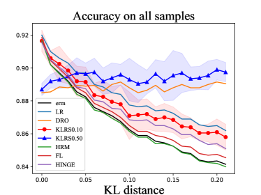
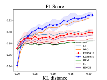
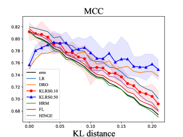
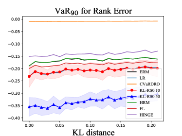
Figure 1: Results of Label Distribution Shift Experiment

5.2 Long-Tailed Learning

Long-tailed learning can be seen as a special case of distribution shift problems, where the class distribution in the training data is skewed while the the test class distribution is evenly distributed. Existing models that use average in-sample performance as the optimization criterion can be easily biased towards dominant classes and perform poorly on minority classes. Our KL-RS model can be integrated into existing methods and help alleviate this issue to enhance overall performance as well as performance in minority classes.

To account for distribution shift in class proportions, we adopt our Hierarchical KL-RS formulation in (10). The group variable is specified by the class label in the data. For simplicity, we consider a baseline case where the proportionality factor in the objective function of Problem (10) is given as $w=0$. This implicitly assumes that distribution shift only happens at the class proportion level while there exists no shift in the distribution of covariates. We conduct experiments on popular artificial datasets for long-tailed learning: CIFAR10 (LT) and CIFAR100 (LT) [9]. These datasets are generated from CIFAR10 and CIFAR100 by Long-Tail strategy. The LT strategy uses a parameter $\rho$ to control the ratio between the size of the most common and most rare classes. The LT strategy performs downsampling on the samples under each class, resulting in a geometric progression of sample quantities across labels. We implement ERM [66], Focal [40], Ldam [9], and CVaRDRO [15] as our benchmarks. For brevity, we relegate the details of the experiment setting and benchmark models to Appendix D.2.

In this experiment, we use ResNet-32 as our model and present the performance comparison results in Table 1, where we include the standard deviation of the metrics in the brackets. Experiment results indicate that our KL-RS model can improve performance over ERM and CVaRDRO benchmarks. When combined with benchmark algorithms including Focal and Ldam models, our KL-RS model can lead to further improvements. For example, the KL-RS Ldam model achieves the highest average and worst-case accuracy in CIFAR10 (LT) dataset. Similarly, the best performing models in CIFAR100 (LT) dataset are KL-RS Focal and KL-RS Ldam.

Additionally, the KL-RS model leads to more pronounced improvement over benchmarks when the long-tail distribution is more skewed, i.e., when $\rho$ becomes smaller. As we can observe from the results when the imbalanced factor is $\rho=0.01$, the improvement attained by the KL-RS Ldam model over other models is on average 14$\%$ on CIFAR10 (LT) and 13$\%$ on CIFAR100 (LT).

Table 1: Results of Long-Tailed Learning

Dataset	$\rho$	0.1		0.01
	Algorithm	average acc	worst acc	average acc	worst acc
CIFAR10 (LT)	ERM	74.93(0.90)	65.77(1.55)	52.01(0.63)	14.72(2.28)
	KL-RS	76.28(0.83)	66.43(0.26)	61.80(0.42)	50.32(0.60)
	CVaRDRO	75.25(1.32)	66.83(0.80)	53.66(0.99)	10.46(4.15)
	Focal	73.55(1.23)	62.34(4.52)	50.83(0.79)	14.35(1.72)
	KL-RS Focal	74.81(0.70)	63.81(2.05)	59.30(1.36)	48.98(0.51)
	Ldam	81.86(0.52)	71.60(1.02)	59.61(1.83)	9.46(4.37)
	KL-RS Ldam	82.87(0.44)	75.06(1.17)	70.68(0.13)	60.96(1.99)
CIFAR100 (LT)	ERM	40.28(0.75)	1.98(0.99)	24.84(0.49)	0.00(0.00)
	KL-RS	41.86(0.54)	15.18(1.14)	27.82(0.63)	0.00(0.00)
	CVaRDRO	39.55(2.34)	2.75(1.06)	24.74(1.53)	0.00(0.00)
	Focal	40.30(0.49)	2.31(1.14)	25.15(0.56)	0.00(0.00)
	KL-RS Focal	40.67(0.82)	13.53(3.02)	27.69(1.15)	0.00(0.00)
	Ldam	42.85(1.14)	0.00(0.00)	27.10(1.03)	0.00(0.00)
	KL-RS Ldam	45.65(0.79)	11.55(2.49)	31.44(1.21)	0.00(0.00)

5.3 Fair PCA

Principal Component Analysis (PCA) is one of the most fundamental dimension reduction algorithm in representation learning [64]. In [59], authors show that standard PCA will exaggerate the reconstruction error in one subpopulation over other subpopulations, which can have an equal size, in real-word dataset. Fair PCA is a novel method that aims to learn low dimensional representations and obtain uniform performance over all subpopulations [64; 32]. The fair PCA model can be formulated as a minimax problem and relaxed into a semi-definite program which can be solved by off-the-shelf solvers.

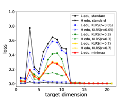
(a) Performance of different subgroups

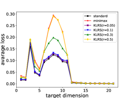
(b) Average performance

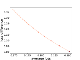
(c) Average vs. Difference

Figure 2: Fair PCA

As an alternative to the fair PCA model, we adopt our KL-RS paradigm to PCA tasks for balancing the performance difference over different subpopulation groups. Similar to [59], we adopt reconstruction error as the loss function. For a matrix $Y\in\mathbb{R}^{a\times n}$, the loss incurred by projecting it to a rank-$d$ matrix $Z\in\mathbb{R}^{a\times n}$ is given by $\|Y-Z\|_{F}^{2}-\|Y-\hat{Y}\|_{F}^{2}$, where $\hat{Y}\in\mathbb{R}^{a\times n}$ is the optimal rank-d approximation of $Y$. Let $\bar{l}$ and $\underline{l}$ denote the maximum and minimum losses among of subgroups, respectively. The target parameter in the KL-RS model can be intuitively set as a convex combination of $\bar{l}$ and $\underline{l}$, i.e., $\tau=r\bar{l}+(1-r)\underline{l},~{}0\leq r\leq 1$. We can tune the hyperparameter $\tau$ conveniently by adjusting the parameter $r$. As the value of parameter $r$ increases, we tend to obtain a projection matrix with more uniform performance across all subgroups. We implement KL-RS PCA with different parameter $r$ on Default Credit dataset [71], which consists of two subgroups (high vs. low education). The benchmark models are standard PCA and Fair PCA [59]. We relegate further details of the experiment setting to Appendix D.3.

We plot the out-of-sample results in Figure 2. The x-axis represents different dimensions, i.e., the value of $n$. In Figure 2(a), we plot the gap between the losses incurred in two subgroups under different models. We observe that the KL-RS model helps reducing this gap as $r$ increases. This is not attained for free. As we observe from Figure 2(b), we may suffer from a higher average loss if we are overly concerned with “fairness”. Nevertheless, we can obtain satisfactory average performance and fairness when $r$ is small. Such a trade-off is inherent in robust decision making. This is also discussed in fairness machine learning [35]. The advantage lies in our algorithm’s ability to smoothly control this trade-off.

6 Conclusion

We investigate a Kullback–Leibler-divergence-based robust satisficing model under a general loss function, extending the scope of existing literature in various aspects. Especially, this work makes several substantial contributions to the broader robust satisficing methodological framework in machine learning community, presenting new research directions and opportunities.

This paper still contains many areas worth further exploration. Firstly, extending from specific KL divergences to more general $\phi$-divergences is an avenue for future research. Simplifying and optimizing the dual forms of more general $\phi$-divergences are important points to investigate. Another aspect is exploring hierarchical structures. This paper only introduces hierarchical KL-RS, but utilizing such structures for modeling machine learning problems has not yet been explored.

Additionally, our research makes minimal assumptions about the true distribution $\mathbb{P}^{*}$, leading to relatively general conclusions. When our KL-RS framework is applied to specific problems, the true distribution may exhibit more definite characteristics, such as a normal distribution or a Bernoulli distribution. In these cases, the expression of our problem might be further simplified and presented in a more insightful mathematical form. Exploring whether KL-RS can yield more insightful conclusions in more specific machine learning tasks compared to general cases might be a direction for future research.

Appendix A Analytical Interpretations

Empirical mean-variance trade-off. When the reference distribution is given by a normal distribution, the KL-RS model (7) becomes an empirical mean-variance constrained model. As a concrete example, let us consider a linear loss $l(\boldsymbol{\theta},\tilde{\boldsymbol{z}})=\boldsymbol{\theta}^{\top}\tilde{\boldsymbol{z}}$ and $\tilde{\boldsymbol{z}}\sim\hat{\mathbb{P}}=N(\mu,\Sigma)$, and the constraint of the KL-RS model (7) becomes

$$\hat{R}(\boldsymbol{\theta},\lambda)=\lambda\log\left(\mathbb{E}_{\hat{\mathbb{P}}}\left[\exp\left(l(\boldsymbol{\theta},\tilde{\boldsymbol{z}})/\lambda\right)\right]\right)=\boldsymbol{\theta}^{\top}\mu+\frac{\boldsymbol{\theta}^{\top}\Sigma\boldsymbol{\theta}}{2\lambda}\leq\tau.$$

As $\boldsymbol{\theta}^{\top}\mu$ and $\boldsymbol{\theta}^{\top}\Sigma\boldsymbol{\theta}$ are the mean and variance of $\boldsymbol{\theta}^{\top}\tilde{\boldsymbol{z}}$, the KL-RS model robustify the solution by increasing the weight of the variance as much as possible while ensuring that the weighted sum of mean and variance is bounded below the tolerance $\tau$. In fact, this observation holds for any distribution of $\bm{\tilde{z}}$ if $\tau$ is a litter larger than $E_{0}$, as stated in the following proposition.

Assumption A.1.

$\mathbb{E}_{\hat{\mathbb{P}}}[l(\boldsymbol{\theta},\tilde{\boldsymbol{z}})]\leq M_{1},\forall\boldsymbol{\theta}\in\Theta$.

Assumption A.2.

$0<\epsilon\leq\mathbb{V}_{\hat{\mathbb{P}}}[l(\boldsymbol{\theta},\tilde{\boldsymbol{z}})]\leq M_{2},\forall\boldsymbol{\theta}\in\Theta$.

Proposition A.3.

Under the Assumption A.1 and Assumption A.2, for any $\boldsymbol{\theta}\in\Theta$, we can choose $\tau=\mathbb{E}_{\hat{\mathbb{P}}}[l(\hat{\boldsymbol{\theta}}_{N},\tilde{\boldsymbol{z}})]+\frac{1}{b}\mathbb{V}_{\hat{\mathbb{P}}}[l(\hat{\boldsymbol{\theta}}_{N},\tilde{\boldsymbol{z}})]$ and $b>\max\left\{1,\frac{2e(M_{1}+M_{2})}{\epsilon}\mathbb{V}_{\hat{\mathbb{P}}}[l(\hat{\boldsymbol{\theta}}_{N},\tilde{\boldsymbol{z}})]\right\}$ where $\hat{\boldsymbol{\theta}}_{N}=\arg\min_{\boldsymbol{\theta}}\mathbb{E}_{\hat{\mathbb{P}}}[l(\boldsymbol{\theta},\tilde{\boldsymbol{z}})]$. Then any feasible $\lambda$ of (6) must satisfy $\lambda\geq\frac{b\epsilon}{2e\mathbb{V}_{\hat{\mathbb{P}}}[l(\hat{\boldsymbol{\theta}}_{N},\tilde{\boldsymbol{z}})]}$.

Proposition A.4.

If $\lambda$ is large enough, we have $\hat{R}(\boldsymbol{\theta},\lambda)=\mathbb{E}_{\hat{\mathbb{P}}}[l(\boldsymbol{\theta},\tilde{\boldsymbol{z}})]+\frac{1}{2\lambda}\mathbb{V}_{\hat{\mathbb{P}}}[l(\boldsymbol{\theta},\tilde{\boldsymbol{z}})]+o(\frac{1}{\lambda^{2}})$, where $\mathbb{V}_{\hat{\mathbb{P}}}[l(\boldsymbol{\theta},\tilde{\boldsymbol{z}})]$ is the variance of $l(\boldsymbol{\theta},\tilde{\boldsymbol{z}})$.

We note that the tolerance $\tau$ selected to marginally exceed empirical loss $\mathbb{E}_{\hat{\mathbb{P}}}[l(\boldsymbol{\theta},\tilde{\boldsymbol{z}})]$ necessitates a significant large $\lambda$, thus transforming the KL-RS model into a mean-variance constrained optimization paradigm.

Prioritization on large losses. The KL-RS model magnifies the impact of samples with large losses (i.e., points that deviate significantly from the estimated values) as value of $\lambda$ decreases. For an illustrative example, we examine two extreme cases of $\hat{R}(\boldsymbol{\theta},\lambda)$ as $\lambda\to 0^{+}$ and $\lambda\to\infty$ demonstrated below:

$${\lim_{\lambda\to 0^{+}}}\hat{R}(\boldsymbol{\theta},\lambda)=\max_{i\in[N]}l(\hat{\boldsymbol{z}}_{i},\boldsymbol{\theta}),\quad\displaystyle{\lim_{\lambda\to+\infty}}\hat{R}(\boldsymbol{\theta},\lambda).=\mathbb{E}_{\hat{\mathbb{P}}}[l(\tilde{\boldsymbol{z}},\boldsymbol{\theta})]$$

As we see, when $\lambda$ approaches zero, the KL-RS model primarily addresses the extreme case. Conversely, as $\lambda$ tends towards infinity, the model puts an equal weight to all samples, reducing to an empirical optimization model (3).

Intuitively, when $\lambda$ decreases from $\infty$ to $0$ gradually, the KL-RS model distributes its attention from equally across all samples to the worst-case sample. In fact, we can quantify this effect by the following proposition.

Proposition A.5.

For a given $\lambda>0$, we obtain the optimal distribution $\mathbb{P}_{0}^{*}$ with

$$\tilde{\boldsymbol{z}}_{0}^{*}\sim\mathbb{P}_{0}^{*}=\arg\sup_{\mathbb{P}\ll\hat{\mathbb{P}}}\mathbb{E}_{\mathbb{\mathbb{P}}}[l(\boldsymbol{\theta},\tilde{\boldsymbol{z}})]-\lambda D_{KL}(\mathbb{\mathbb{P}}\|\hat{\mathbb{P}}).$$

where $\mathbb{P}_{0}^{*}(\tilde{\boldsymbol{z}}_{0}^{*}=\hat{\boldsymbol{z}}_{i})=\frac{\exp(l(\boldsymbol{\theta},\hat{\boldsymbol{z}}_{i})/\lambda)}{N\cdot\mathbb{E}_{\hat{\mathbb{P}}}[\exp(l(\boldsymbol{\theta},\tilde{\boldsymbol{z}})/\lambda)]}$ for all $i\in[N]$.

We remark that the constraint of KL-RS model in (6) can be reformulated as $\sup_{\mathbb{P}_{0}\ll\hat{\mathbb{P}}}\{\mathbb{E}_{\mathbb{\mathbb{P}}}[l(\boldsymbol{\theta},\tilde{\boldsymbol{z}})]-\lambda D_{KL}(\mathbb{\mathbb{P}}\|\hat{\mathbb{P}})\}\leq\tau$, and further simplified into $\mathbb{E}_{\mathbb{P}_{0}^{*}}[l(\boldsymbol{\theta},\tilde{\boldsymbol{z}})]-\lambda D_{KL}(\mathbb{P}_{0}^{*}\|\hat{\mathbb{P}})\leq\tau$ by Proposition A.5. Now, we observe that the KL-RS model amplifies the influence of samples with large losses, where $\mathbb{P}_{0}^{*}(\tilde{\boldsymbol{z}}_{0}^{*}=\hat{\boldsymbol{z}}_{i})$ serves as the relative weight attributed to each sample.

A.1 An Illustrative Example

In this subsection, we use a simple example to illustrate the above-mentioned interpretations.

Consider that 100 two-dimensional data points are generated from two distributions. In Figure 3, 80 data points clustered in the top-left corner are sampled from a Normal distribution with mean $(-1,2)$ and variance $0.4I$; the remaining 20 points clustered it the bottom-right corner are sampled from another Normal distribution with mean $(0.2,0.2)$ and variance $0.6I$. In addition, we highlight the geometric mean of these points in pink and the arithmetic mean in yellow.

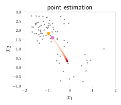
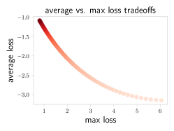
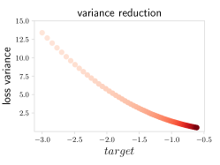
Figure 3: Performance evaluations across varied $\tau$

We conduct the KL-RS model training with loss function $l(\boldsymbol{\theta},\tilde{\boldsymbol{z}})=\frac{1}{2}(\boldsymbol{\theta}-\tilde{\boldsymbol{z}})^{2}$ for the point estimation. As we vary the tolerance parameter $\tau$ from the empirical loss to infinity, the corresponding optimal solution $\boldsymbol{\theta}^{*}(\tau)$ also varies. In Figure 3, points are shaded darker to denote $\boldsymbol{\theta}^{*}(\tau)$ with larger $\tau$.

In Figure 3, larger $\tau$ values lead to estimated points approaching minority class of points, consequently reducing maximum sample loss. This observation is also articulated in Figure 3, where the average loss gradually increases while the maximum sample loss decreases. Figure 3 illustrates a reduction in the variance of empirical loss with increasing $\tau$, which aligns with the interpretation of empirical mean-variance trade-off.

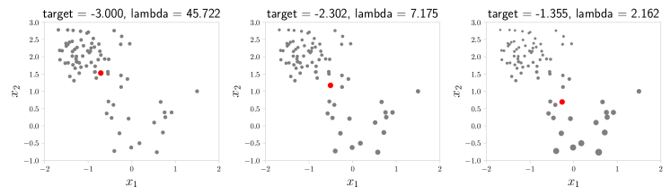
Figure 4: Weights attributed to samples

We select three target $\tau$ and demonstrate the corresponding weights attributed to samples based on Proposition A.5 in Figure 4. The size of each data point is proportional to the weight of this sample. When $\tau=-3$, the KL-RS model assigns nearly uniform weights to all samples (left panel). When $\tau=-1.355$, it is obvious that the KL-RS model amplifies the influence of samples with large losses (right panel), which aligns with the interpretation of prioritizing samples with large losses.

Appendix B The Advantages of Feasibility Detection of the KL-RS Model

Our algorithm 1 demonstrates two pivotal advantages: unbiasedness and normalization, which effectively avoid the bias of gradient estimation and mitigate the scaling concern.

Problem of biasedness. The framework of tilted empirical risk minimization (see e.g. [39, 38, 54]) optimizes $\hat{R}(\boldsymbol{\theta},\lambda)$ directly with the gradient

$$\nabla_{\boldsymbol{\theta}}\hat{R}(\boldsymbol{\theta},\lambda)=\frac{1}{\lambda}\sum_{i\in[N]}\frac{\exp(l(\boldsymbol{\theta},\hat{\boldsymbol{z}}_{i})/\lambda)}{\sum_{j\in[N]}\exp(l(\boldsymbol{\theta},\hat{\boldsymbol{z}}_{j})/\lambda)}\cdot\nabla_{\boldsymbol{\theta}}l(\boldsymbol{\theta},\hat{\boldsymbol{z}}_{i}).$$

Note that the gradient of each sample is reweighted by $\frac{1}{\lambda}\frac{\exp(l(\boldsymbol{\theta},\hat{\boldsymbol{z}}_{i}))}{\sum_{j\in[N]}\exp(l(\boldsymbol{\theta},\hat{\boldsymbol{z}}_{j})/\lambda)}$. The estimation of the denominator presents a significant challenge in a stochastic or mini-batch setting because a straightforward estimation of the exponential sum introduces bias. To alleviate this issue, a common strategy involves retaining an additional estimator for the denominator at the expense of extra sampling [39, 38, 54].

Problem of scaling. A straightforward approach to rectifying the biased gradient estimator involves directly optimizing a component of $\hat{R}(\boldsymbol{\theta},\lambda)$:

$$\min_{\boldsymbol{\theta}\in\Theta}\hat{R}(\boldsymbol{\theta},\lambda)\quad\Longleftrightarrow\quad\min_{\boldsymbol{\theta}\in\Theta}\mathbb{E}_{\hat{\mathbb{P}}}\left[\exp\left(\frac{l(\boldsymbol{\theta},\tilde{\boldsymbol{z}})}{\lambda}\right)\right],$$

with the gradient

$$\nabla_{\boldsymbol{\theta}}\mathbb{E}_{\hat{\mathbb{P}}}\left[\exp\left(\frac{l(\boldsymbol{\theta},\tilde{\boldsymbol{z}})}{\lambda}\right)\right]=\frac{1}{\lambda N}\sum_{i\in[N]}\exp\left(\frac{l(\boldsymbol{\theta},\hat{\boldsymbol{z}}_{i})}{\lambda}\right)\nabla_{\boldsymbol{\theta}}l(\boldsymbol{\theta},\hat{\boldsymbol{z}}_{i}).$$ (11)

Although mini-batch gradient of (11) is an unbiased estimator, the scale of this gradient is significantly influenced by $\exp\left(\frac{l(\boldsymbol{\theta},\hat{\boldsymbol{z}}_{i})}{\lambda}\right)$. In practice, the amplification of gradient magnitude may induce numerical errors. Conversely, a diminished gradient may cause the objective function value to decrease slowly or remain stagnant, especially when the loss is relatively small after several iterations.

Our approach. The objective function of our approach is

$$\min_{\boldsymbol{\theta}\in\Theta}\mathbb{E}_{\hat{\mathbb{P}}}[\exp\left(\frac{l(\boldsymbol{\theta},\tilde{\boldsymbol{z}})-\tau}{\lambda}\right)],$$

with the gradient

$$\nabla_{\boldsymbol{\theta}}\mathbb{E}_{\hat{\mathbb{P}}}\left[\exp\left(\frac{l(\boldsymbol{\theta},\tilde{\boldsymbol{z}})-\tau}{\lambda}\right)\right]=\frac{1}{\lambda N}\sum_{i\in[N]}\frac{\exp(l(\boldsymbol{\theta},\hat{\boldsymbol{z}}_{i})/\lambda)}{\exp(\tau/\lambda)}\nabla_{\boldsymbol{\theta}}l(\boldsymbol{\theta},\hat{\boldsymbol{z}}_{i}).$$ (12)

In a stochastic or mini-batch regime, our gradient estimator demonstrates unbiasedness. Moreover, we observe that our gradient (12) is normalized by $\exp(\tau/\lambda)$ compared to vanilla (11). Considering that the $t$th iterate satisfies $\sum_{i\in[N]}\exp(\frac{l(\boldsymbol{\theta}_{t-1},\hat{\boldsymbol{z}}_{i})}{\lambda})\leq\exp(\tau/\lambda)$, the update from $\boldsymbol{\theta}_{t-1}$ to $\boldsymbol{\theta}_{t}$ is more stable.

In summary, the effective and stable performance stems from the KL-RS setting, a feature absent in the tilted empirical risk minimization framework.

Appendix C Algorithm development for Hierarchical KL-RS Model

We consider the scope of alternative optimization. Supposing that $(\lambda_{1},\lambda_{2})$ is fixed, we shall verify the feasibility of $(\lambda_{1},\lambda_{2})$. Note that the constraint

$$\hat{\mathbf{R}}(\boldsymbol{\theta},\lambda_{1},\lambda_{2})\triangleq \lambda_{1}\log\left(\mathbb{E}_{\hat{\mathbb{P}}_{\tilde{\boldsymbol{g}}}}\left[\exp\left(\lambda_{2}\log\left(\mathbb{E}_{\hat{\mathbb{P}}_{\tilde{\boldsymbol{z}}|\tilde{\boldsymbol{g}}}}\exp\left(l(\boldsymbol{\theta},\tilde{\boldsymbol{z}})/\lambda_{2}\right)\right)/\lambda_{1}\right)\right]\right)\leq\tau$$

$$\Longleftrightarrow\quad \mathbb{E}_{\hat{\mathbb{P}}_{\tilde{\boldsymbol{g}}}}\left[\exp\left(\lambda_{2}\log\left(\mathbb{E}_{\hat{\mathbb{P}}_{\tilde{\boldsymbol{z}}|\tilde{\boldsymbol{g}}}}\exp\left(l(\boldsymbol{\theta},\tilde{\boldsymbol{z}})/\lambda_{2}\right)\right)/\lambda_{1}\right)\right]\leq\exp(\tau/\lambda_{1})$$

$$\Longleftrightarrow\quad \mathbb{E}_{\hat{\mathbb{P}}_{\tilde{\boldsymbol{g}}}}\left[\exp\left(\frac{\lambda_{2}}{\lambda_{1}}\log\left(\mathbb{E}_{\hat{\mathbb{P}}_{\tilde{\boldsymbol{z}}|\tilde{\boldsymbol{g}}}}\exp(l(\boldsymbol{\theta},\tilde{\boldsymbol{z}})/\lambda_{2})\right)-\frac{\tau}{\lambda_{1}}\right)\right]\leq 1$$

$$\Longleftrightarrow\quad \mathbb{E}_{\hat{\mathbb{P}}_{\tilde{\boldsymbol{g}}}}\left[\exp\left(\frac{\lambda_{2}}{\lambda_{1}}\left(\log\left(\mathbb{E}_{\hat{\mathbb{P}}_{\tilde{\boldsymbol{z}}|\tilde{\boldsymbol{g}}}}\exp(l(\boldsymbol{\theta},\tilde{\boldsymbol{z}})/\lambda_{2})\right)-\frac{\tau}{\lambda_{2}}\right)\right)\right]\leq 1$$

$$\Longleftrightarrow\quad \mathbb{E}_{\hat{\mathbb{P}}_{\tilde{\boldsymbol{g}}}}\left[\exp\left(\frac{\lambda_{2}}{\lambda_{1}}\log\left(\mathbb{E}_{\hat{\mathbb{P}}_{\tilde{\boldsymbol{z}}|\tilde{\boldsymbol{g}}}}\exp\left(\frac{l(\boldsymbol{\theta},\tilde{\boldsymbol{z}})-\tau}{\lambda_{2}}\right)\right)\right)\right]\leq 1$$

$$\Longleftrightarrow\quad \mathbb{E}_{\hat{\mathbb{P}}_{\tilde{\boldsymbol{g}}}}\left[\left(\mathbb{E}_{\hat{\mathbb{P}}_{\tilde{\boldsymbol{z}}|\tilde{\boldsymbol{g}}}}\exp\left(\frac{l(\boldsymbol{\theta},\tilde{\boldsymbol{z}})-\tau}{\lambda_{2}}\right)\right)^{\frac{\lambda_{2}}{\lambda_{1}}}\right]\leq 1.$$

Therefore, to assess the viability of the hierarchical KL-RS model, it is imperative to tackle the conditional stochastic optimization problem:

$$\min_{\boldsymbol{\theta}}\mathbb{E}_{\hat{\mathbb{P}}_{\tilde{\boldsymbol{g}}}}\left[h\left(\mathbb{E}_{\hat{\mathbb{P}}_{\tilde{\boldsymbol{z}}|\tilde{\boldsymbol{g}}}}\left[f(\boldsymbol{\theta},\tilde{\boldsymbol{z}};\lambda_{2})\right];\lambda_{1},\lambda_{2}\right)\right]$$

with $h(x;\lambda_{1},\lambda_{2})\triangleq x^{\frac{\lambda_{2}}{\lambda_{1}}}$ and $f$ is defined in Section 4.1. Generally speaking, conditional stochastic optimization problem is computationally challenging in practice, because the estimator of the gradient is often biased [27, 30, 28]. At the early stage of our experiment, we adopt the vanilla biased stochastic gradient method introduced by [30]. It appears that this method often encounters difficulties when training neural networks with batch normalization (BN) layers, especially when there are significant disparities in means and variances among different classes in Section 5.2. To improve and stabilize the performance, we tailor the biased stochastic gradient method by introducing a hierarchical mini-batch strategy, resulting in the following algorithm. We can verify that the convergence rate of our algorithm aligns with the result in [30] by a constant factor.

1 Input: $\lambda_{1},\lambda_{2}$

2 Initialization: group batch size $M_{1}$, batch size within group $M_{2}$, step size $\alpha$

3 while stopping criteria not reached do

4      Sample $\hat{\boldsymbol{g}}_{i}$ uniformly random from $\tilde{\boldsymbol{g}}$ with batch size $M_{1}$;

5      for $i=1$ to $M_{1}$ do

6           For each given $\hat{\boldsymbol{g}}_{i}$, sample $\hat{\boldsymbol{z}}_{i,j}$ uniformly random from $\tilde{\boldsymbol{z}}|\hat{\boldsymbol{g}}_{i}$ with batch size $M_{2}$;

7           Construct $\bar{l}_{i}\triangleq\frac{1}{M_{2}}\sum_{j\in[M_{2}]}l(\boldsymbol{\theta},\hat{\boldsymbol{z}}_{i,j}),\quad\bar{\mathrm{l}}_{i}\triangleq\frac{1}{M_{2}}\sum_{j\in[M_{2}]}\nabla l(\boldsymbol{\theta},\hat{\boldsymbol{z}}_{i,j})$

8           end for

9          Construct $\nabla F\triangleq\frac{1}{M_{1}}\sum_{i\in[M_{1}]}h^{\prime}(\bar{l}_{i};\lambda_{1},\lambda_{2})\cdot\bar{\mathrm{l}}_{i}$

10           Update $\boldsymbol{\theta}\leftarrow\boldsymbol{\theta}-\alpha\nabla F$

11           end while

Output: Boolean$\left(\mathbb{E}_{\hat{\mathbb{P}}_{\tilde{\boldsymbol{g}}}}\left[h\left(\mathbb{E}_{\hat{\mathbb{P}}_{\tilde{\boldsymbol{z}}|\tilde{\boldsymbol{g}}}}\left[f(\boldsymbol{\theta},\tilde{\boldsymbol{z}};\lambda_{2})\right];\lambda_{1},\lambda_{2}\right)\right]\leq 1\right)$

Algorithm 3 Feasibility of the hierarchical KL-RS model $(\lambda_{1},\lambda_{2})$

Back to the scope of alternative optimization, supposing that $\boldsymbol{\theta}$ is fixed, we first propose desirable properties of $\hat{\mathbf{R}}(\boldsymbol{\theta},\lambda_{1},\lambda_{2})$ in the following proposition.

Proposition C.1.

$\hat{\mathbf{R}}(\boldsymbol{\theta},\lambda_{1},\lambda_{2})$ is convex on $(\lambda_{1},\lambda_{2})$, and non-increasing with respect to $\lambda_{2}$.

Now, supposing that $\lambda_{1}$ is fixed, we consider the following sub-problem 13:

$$H(\lambda_{1})= \min_{\boldsymbol{\theta},\lambda_{2}\geq 0}\lambda_{2}$$ (13)

s.t. $$\hat{\mathbf{R}}(\boldsymbol{\theta},\lambda_{1},\lambda_{2})\leq\tau.$$

Similar to Algorithm 2, we can develop a bisection method to solve it due to monotonicity.

1 Input: $\lambda_{1}$

Initialization :  $\underline{\lambda}=0$, a positive value $\lambda_{0}$, a precision $\epsilon>0$

2 while  Algorithm 3($\lambda_{1},\lambda_{0}$) == False do

3     $\underline{\lambda}\leftarrow\lambda_{0}$, $\lambda_{0}\leftarrow 2\lambda_{0}$

4      end while

5          $\overline{\lambda}=\lambda_{0}$

6      while  $\overline{\lambda}-\underline{\lambda}\geq\epsilon$ do

7          $\lambda_{\text{mid}}=(\overline{\lambda}+\underline{\lambda})/2$

8           if  Algorithm 3($\lambda_{1},\lambda_{\text{mid}}$)==True  then

9               $\overline{\lambda}=\lambda_{\text{mid}}$

10                end if

11               else

12                    $\underline{\lambda}=\lambda_{\text{mid}}$

13                     end if

14                    

15                     end while

Output: $\lambda_{\text{mid}}$

Algorithm 4 Find optimal $\lambda_{2}$ by bisection method ($\lambda_{1}$)

According to the sub-problem 13, we can reformulate the hierarchical KL-RS problem as

$$\min_{\lambda_{1}\geq 0}\;\;\lambda_{1}+wH(\lambda_{1}).$$

We can verify that $\lambda_{1}+wH(\lambda_{1})$ is a convex function on $\lambda_{1}$ with $w>0$ by proposition C.1, which can be solved by the golden-ratio search. In all, we propose our algorithm 5 to solve the hierarchical KL-RS.

Initialization :  a precision $\epsilon>0$, $\gamma=0.382$, ${\lambda_{l}}=\lambda_{\min}$, ${\lambda_{r}}=\lambda_{\max}$

1 while  $\lambda_{r}-\lambda_{l}\geq\epsilon$ do

2      $\lambda^{\prime}_{l}=\lambda_{l}+\gamma(\lambda_{r}-\lambda_{l})$,  $\lambda^{\prime}_{r}=\lambda_{l}+(1-\gamma)(\lambda_{r}-\lambda_{l})$

3      $\lambda^{(2)}_{l}=$Algorithm 4($\lambda^{\prime}_{l}$),  $\lambda^{(2)}_{r}=$Algorithm 4($\lambda^{\prime}_{r}$)

4      if  $\lambda^{\prime}_{l}+w\lambda^{(2)}_{l}\leq\lambda^{\prime}_{r}+w\lambda^{(2)}_{r}$ then

5          ${\lambda_{r}}=\lambda^{\prime}_{r}$

6           end if

7          else

8               ${\lambda_{l}}=\lambda^{\prime}_{l}$

9                end if

10               

11                end while

Output: $\lambda_{\text{mid}}$

Algorithm 5 Solve the hierarchical KL-RS by golden-ratio search

Appendix D Details for Section 5

D.1 Details of Section 5.1

D.1.1 Background

Label distribution shift is a special case of the out-of-distribution (OOD) problem, where the label distribution in the training dataset does not reflect what is observed during testing. For example, this is commonly seen in predicting diseases based on symptoms. Suppose a model is trained in dermatology hospital and used in a skin disease hospital, there would be label distribution shift. Such label distribution will degrade model performance significantly. Some works assumed that we can obtain some unlabelled test samples so that we can use them to estimate the shift in distribution. However, unlabelled test samples are not always accessible and a trained model may be deployed on many environments. Hence, a model that is robust to label distribution shift is desired.

D.1.2 Experiment Setting

The HIV-1 dataset was first investigated in [15]. This dataset contains 6590 samples, with 1360 positive samples and 5230 negative samples. In this experiment, we adopt a linear model with a sigmoid layer and the cross-entropy loss function.

To obtain test datasets with varying KL divergences from the training set, we employed the following method. First, we randomly sampled 329 samples from the positive samples to construct a positive sample pool. Then, we sampled 330 samples from the negative samples to construct a negative sample pool. Then, the remaining samples were used as the training samples. Third, based on the given KL divergence value, we calculate the proportion of positive and negative samples on the test set using the distribution of positive and negative samples on the training set as the reference distribution. Finally, according to the calculated proportions, sample 400 instances from positive sample pool and negative sample pool to construct a test dataset to evaluate the performance of model. Repeat the sampling process and evaluation process for multiple times with different ramdom seeds.

Experiment platform. The experiments are conducted on a Windows11 system with 13th Gen Intel(R) Core(TM) i7-13700H 2.40 GHz processor and 32.0 GB memory. No graphics card is used in this experiments.

D.1.3 Hyperparameter Tuning

We referred to [39] for selecting the hyperparameters in our benchmark. For algorithms with hyperparameters, we use the hyperparameters chosen in the original paper where the algorithm was proposed as the baseline, perform a geometric or arithmetic search over five values, and then present the results for the hyperparameter with best MCC performance. Interestingly, we initially expected that different hyperparameters might perform better at different distribution shift distances. However, the actual results often show that a particular hyperparameter tends to perform better across all distances than other hyperparameter.

For CVaRDRO, we choose 4.0 from $\{0.25,0.50,1.00,2.00,4.00\}$ as our hyperparamert. For FL, we choose 0.25 from $\{0.25,0.5,1.0,2,4\}$. For HINGE, we choose 0.5 from $\{0.5,1,2,4,8\}$. For HRM, we choose 0.00 from $\{0.00,0.20,0.40,0.60,0.80\}$. There is no hyperparameter for LR. As for our KL-RS, we set $\tau=(1+\epsilon)E_{0}$ with $\{0.10,0.20,0.30,0.40,0.50\}$. We present the result with $\epsilon=0.10$ and $\epsilon=0.50$.

D.1.4 Computation Time

For each algorithm, we update 10000 times. We conduct each optimization algorithm five times and report the mean and standard deviation of the computation time in table 2. We do not present the computation time for HINGE because it is computed using the ‘LinearSVC‘ package from ‘sklearn.svm‘. The other algorithms are based on gradient descent, making the computation time for HINGE not directly comparable.

Even thought the computation time of KL-RS is longer than ERM, compared with other benchmarks, extra computation burdern is mild.

Table 2: Computation Time for Label Distribution Shift

Algorithm	KL-RS0.10	KL-RS0.50	ERM	CVaRDRO	FL	HRM	LR
Average Time(s)	5.69	5.62	2.66	16.186	5.88	21.66	49.17
Std Time(s)	0.11	0.19	0.06	0.22	0.41	0.10	0.41

D.1.5 Evaluation Metric

We adopt a variety of metrics to evaluate the model’s performance, including F1 score, Matthews Correlation Coefficient (MCC), accuracy on rare samples (Acc1), accuracy on common sample (Acc0), and accuracy on overall samples (Acc). Particularly, MCC is an evaluation metric tailored for binary classification task with imbalanced labels with the following definition,

Definition D.1 (Matthews Correlation Coefficient (MCC)).

$$MCC\triangleq\frac{TP\times TN-FP\times FN}{\sqrt{(TP+FP)(TP+FN)(TN+FP)(TN+FN)}},$$ (14)

where $TP$ denotes true positive samples, $TN$ denotes true negative samples, $FP$ denotes false positive samples, and $FN$ denotes false negative samples.

In addition to the classic binary classification evaluation metrics mentioned earlier, we also employ rank error as a metric.

Definition D.2 (Rank Error).

Given a prediction model $h$, a positive sample $x_{+}$ and a negative sample $x_{-}$, the ranking error is defined as

$$\epsilon(h)\triangleq h(x_{-})-h(x_{+}).$$ (15)

For an ideal classifier, it should always assign a higher score to a positive sample compared to a negative sample. When model assigns a larger value to a negative sample, the model makes some mistakes. Smaller rank error is preferred by a binary classification model.

We investigate the Value-at-Risk (VaR) of rank error which is the $\alpha$-quantile of rank error. For a r.v. $\tilde{v}$, its $\alpha$-quantile is $VaR_{\alpha}(\tilde{v})\triangleq\min\{a|\mathbb{P}(\tilde{v}\leq a)\geq\alpha\}$ and its $\alpha$-superquantile is $CVaR_{\alpha}(\tilde{v})\triangleq\mathbb{E}[\tilde{\boldsymbol{z}}|\tilde{\boldsymbol{z}}\geq VaR_{\alpha}(\tilde{v})]$. Both $VaR_{\alpha}(\epsilon(h))$ and $CVaR_{\alpha}(\epsilon(h))$ evaluate the risk of large rank error, which can be interpreted as risk of misclassification. We adopt $VaR_{90}(\epsilon(h))$ and $CVaR_{90}(\epsilon(h))$ as our metric to evaluate our model.

We evaluate the model’s performance on test sets at 21 different KL distances $\{0.00,0.01,\cdots,0.20\}$. For each given distance, we employ 5 random seeds to randomly sample the test sets and record the average metrics. We present the experimental results at distance of 0.00, 0.05, 0.10, 0.15 and 0.20 in Table 3, 4, 5, 6 and 7. We select results from these distances to demonstrate outcomes in three scenarios: no distribution shift, slight shift, and significant shift.

As we have mentioned, KL-RS sacrifices some performance on average to improve the model’s generalization capability.

As the KL distance increases, various metrics for KL-RS0.10 degrade significantly, similar to ERM. However, KL-RS0.10 completely outperforms the ERM approach by achieving comparable in-sample Acc, MCC, and F1 scores, while also outperforming ERM on all metrics except for Acc0 after the distribution shift. KL-RS0.10 achieves a noticeable improvement in generalization with a negligible loss in in-sample performance.

Compared with KLRS0.10, KLRS0.50 improves the generalization ability of model greatly. The KL-RS0.50 model’s performance does not deteriorate rapidly with distribution shifts. It is foreseeable that, as the distance further increases, the various metrics for KL-RS0.50 will not experience significant degradation. However, this strong generalization ability comes at the cost of reduced in-sample performance. When there is no distribution shift or only a slight shift, KL-RS0.50 underperforms compared to ERM in terms of MCC, F1, and Acc.

Table 3: Results Of Label Distribution Shift at Distance 0.00

Algorithm	Statistic	Metric
		Acc1	Acc0	Acc	MCC	F1	$\mbox{VaR}_{90}$	$\mbox{CVaR}_{90}$
ERM	mean	0.807	0.973	0.917	0.814	0.868	-0.189	-0.028
	std	$\pm 0.026$	$\pm 0.003$	$\pm 0.009$	$\pm 0.020$	$\pm 0.016$	$\pm 0.040$	$\pm 0.027$
CVaRDRO	mean	0.875	0.890	0.885	0.751	0.838	-0.009	-0.004
	std	$\pm 0.018$	$\pm 0.006$	$\pm 0.006$	$\pm 0.013$	$\pm 0.009$	$\pm 0.001$	$\pm 0.001$
KL-RS0.10	mean	0.832	0.960	0.916	0.812	0.871	-0.232	-0.048
	std	$\pm 0.018$	$\pm 0.002$	$\pm 0.007$	$\pm 0.015$	$\pm 0.011$	$\pm 0.044$	$\pm 0.031$
KL-RS0.50	mean	0.887	0.888	0.887	0.758	0.843	-0.354	-0.133
	std	$\pm 0.014$	$\pm 0.007$	$\pm 0.004$	$\pm 0.009$	$\pm 0.006$	$\pm 0.038$	$\pm 0.040$
HRM	mean	0.812	0.970	0.916	0.812	0.868	-0.188	-0.027
	std	$\pm 0.024$	$\pm 0.004$	$\pm 0.009$	$\pm 0.020$	$\pm 0.015$	$\pm 0.041$	$\pm 0.027$
FL	mean	0.812	0.973	0.918	0.817	0.871	-0.200	-0.043
	std	$\pm 0.024$	$\pm 0.003$	$\pm 0.008$	$\pm 0.018$	$\pm 0.014$	$\pm 0.036$	$\pm 0.027$
HINGE	mean	0.825	0.962	0.915	0.810	0.869	-0.151	-0.030
	std	$\pm 0.023$	$\pm 0.003$	$\pm 0.008$	$\pm 0.018$	$\pm 0.014$	$\pm 0.015$	$\pm 0.017$
LR	mean	0.834	0.964	0.920	0.820	0.876	-0.232	-0.048
	std	$\pm 0.021$	$\pm 0.003$	$\pm 0.009$	$\pm 0.020$	$\pm 0.015$	$\pm 0.044$	$\pm 0.032$

Table 4: Results Of Label Distribution Shift at Distance 0.05

Algorithm	Statistic	Metric
		Acc1	Acc0	Acc	MCC	F1	$\mbox{VaR}_{90}$	$\mbox{CVaR}_{90}$
ERM	mean	0.806	0.972	0.882	0.780	0.880	-0.169	-0.021
	std	$\pm 0.019$	$\pm 0.006$	$\pm 0.010$	$\pm 0.017$	$\pm 0.011$	$\pm 0.019$	$\pm 0.015$
CVaRDRO	mean	0.880	0.899	0.889	0.778	0.895	-0.008	-0.003
	std	$\pm 0.008$	$\pm 0.016$	$\pm 0.004$	$\pm 0.009$	$\pm 0.003$	$\pm 0.001$	$\pm 0.001$
KL-RS0.10	mean	0.832	0.961	0.891	0.793	0.892	-0.214	-0.041
	std	$\pm 0.017$	$\pm 0.007$	$\pm 0.009$	$\pm 0.016$	$\pm 0.010$	$\pm 0.022$	$\pm 0.018$
KL-RS0.50	mean	0.894	0.899	0.896	0.793	0.903	-0.357	-0.133
	std	$\pm 0.011$	$\pm 0.019$	$\pm 0.007$	$\pm 0.014$	$\pm 0.006$	$\pm 0.027$	$\pm 0.021$
HRM	mean	0.806	0.970	0.881	0.778	0.880	-0.168	-0.020
	std	$\pm 0.016$	$\pm 0.006$	$\pm 0.008$	$\pm 0.013$	$\pm 0.009$	$\pm 0.019$	$\pm 0.015$
FL	mean	0.810	0.972	0.885	0.784	0.883	-0.186	-0.037
	std	$\pm 0.016$	$\pm 0.006$	$\pm 0.008$	$\pm 0.015$	$\pm 0.010$	$\pm 0.017$	$\pm 0.016$
HINGE	mean	0.821	0.964	0.887	0.786	0.887	-0.152	-0.031
	std	$\pm 0.013$	$\pm 0.010$	$\pm 0.006$	$\pm 0.011$	$\pm 0.006$	$\pm 0.017$	$\pm 0.014$
LR	mean	0.836	0.968	0.897	0.804	0.897	-0.217	-0.041
	std	$\pm 0.015$	$\pm 0.004$	$\pm 0.008$	$\pm 0.013$	$\pm 0.008$	$\pm 0.026$	$\pm 0.019$

Table 5: Results Of Label Distribution Shift at Distance 0.10

Algorithm	Statistic	Metric
		Acc1	Acc0	Acc	MCC	F1	$\mbox{VaR}_{90}$	$\mbox{CVaR}_{90}$
ERM	mean	0.798	0.970	0.863	0.744	0.878	-0.164	-0.009
	std	$\pm 0.018$	$\pm 0.010$	$\pm 0.012$	$\pm 0.020$	$\pm 0.012$	$\pm 0.024$	$\pm 0.026$
CVaRDRO	mean	0.881	0.899	0.888	0.768	0.907	-0.008	-0.003
	std	$\pm 0.007$	$\pm 0.017$	$\pm 0.008$	$\pm 0.018$	$\pm 0.007$	$\pm 0.001$	$\pm 0.001$
KL-RS0.10	mean	0.822	0.951	0.871	0.751	0.888	-0.206	-0.027
	std	$\pm 0.016$	$\pm 0.018$	$\pm 0.014$	$\pm 0.028$	$\pm 0.013$	$\pm 0.031$	$\pm 0.031$
KL-RS0.50	mean	0.892	0.894	0.893	0.777	0.912	-0.323	-0.106
	std	$\pm 0.009$	$\pm 0.022$	$\pm 0.012$	$\pm 0.026$	$\pm 0.010$	$\pm 0.029$	$\pm 0.032$
HRM	mean	0.798	0.967	0.862	0.741	0.878	-0.163	-0.008
	std	$\pm 0.015$	$\pm 0.010$	$\pm 0.011$	$\pm 0.020$	$\pm 0.011$	$\pm 0.024$	$\pm 0.026$
FL	mean	0.802	0.970	0.865	0.748	0.881	-0.180	-0.024
	std	$\pm 0.015$	$\pm 0.010$	$\pm 0.010$	$\pm 0.018$	$\pm 0.010$	$\pm 0.022$	$\pm 0.026$
HINGE	mean	0.816	0.955	0.868	0.749	0.885	-0.139	-0.021
	std	$\pm 0.013$	$\pm 0.012$	$\pm 0.011$	$\pm 0.021$	$\pm 0.010$	$\pm 0.030$	$\pm 0.021$
LR	mean	0.828	0.959	0.878	0.765	0.894	-0.205	-0.026
	std	$\pm 0.016$	$\pm 0.016$	$\pm 0.013$	$\pm 0.026$	$\pm 0.012$	$\pm 0.033$	$\pm 0.029$

Table 6: Results Of Label Distribution Shift at Distance 0.15

Algorithm	Statistic	Metric
		Acc1	Acc0	Acc	MCC	F1	$\mbox{VaR}_{90}$	$\mbox{CVaR}_{90}$
ERM	mean	0.801	0.966	0.853	0.716	0.882	-0.162	-0.008
	std	$\pm 0.013$	$\pm 0.007$	$\pm 0.010$	$\pm 0.017$	$\pm 0.009$	$\pm 0.022$	$\pm 0.026$
CVaRDRO	mean	0.886	0.894	0.888	0.753	0.916	-0.008	-0.003
	std	$\pm 0.007$	$\pm 0.045$	$\pm 0.016$	$\pm 0.041$	$\pm 0.011$	$\pm 0.001$	$\pm 0.001$
KL-RS0.10	mean	0.830	0.955	0.869	0.737	0.897	-0.203	-0.024
	std	$\pm 0.010$	$\pm 0.011$	$\pm 0.008$	$\pm 0.015$	$\pm 0.007$	$\pm 0.028$	$\pm 0.031$
KL-RS0.50	mean	0.897	0.892	0.895	0.766	0.922	-0.319	-0.097
	std	$\pm 0.009$	$\pm 0.037$	$\pm 0.014$	$\pm 0.034$	$\pm 0.010$	$\pm 0.032$	$\pm 0.027$
HRM	mean	0.801	0.966	0.853	0.716	0.882	-0.162	-0.006
	std	$\pm 0.012$	$\pm 0.007$	$\pm 0.009$	$\pm 0.016$	$\pm 0.008$	$\pm 0.023$	$\pm 0.026$
FL	mean	0.807	0.966	0.856	0.721	0.885	-0.178	-0.022
	std	$\pm 0.010$	$\pm 0.007$	$\pm 0.008$	$\pm 0.014$	$\pm 0.007$	$\pm 0.020$	$\pm 0.027$
HINGE	mean	0.820	0.958	0.863	0.729	0.892	-0.139	-0.019
	std	$\pm 0.009$	$\pm 0.009$	$\pm 0.008$	$\pm 0.014$	$\pm 0.006$	$\pm 0.030$	$\pm 0.018$
LR	mean	0.833	0.960	0.872	0.745	0.900	-0.201	-0.024
	std	$\pm 0.010$	$\pm 0.008$	$\pm 0.007$	$\pm 0.012$	$\pm 0.006$	$\pm 0.030$	$\pm 0.030$

Table 7: Results Of Label Distribution Shift at Distance 0.20

Algorithm	Statistic	Metric
		Acc1	Acc0	Acc	MCC	F1	$\mbox{VaR}_{90}$	$\mbox{CVaR}_{90}$
ERM	mean	0.803	0.964	0.844	0.683	0.885	-0.159	0.000
	std	$\pm 0.007$	$\pm 0.019$	$\pm 0.010$	$\pm 0.022$	$\pm 0.007$	$\pm 0.022$	$\pm 0.028$
CVaRDRO	mean	0.883	0.917	0.891	0.746	0.924	-0.008	-0.003
	std	$\pm 0.006$	$\pm 0.021$	$\pm 0.008$	$\pm 0.020$	$\pm 0.006$	$\pm 0.001$	$\pm 0.001$
KL-RS0.10	mean	0.831	0.950	0.861	0.704	0.899	-0.199	-0.016
	std	$\pm 0.005$	$\pm 0.020$	$\pm 0.008$	$\pm 0.020$	$\pm 0.006$	$\pm 0.028$	$\pm 0.031$
KL-RS0.50	mean	0.895	0.913	0.900	0.760	0.930	-0.311	-0.085
	std	$\pm 0.005$	$\pm 0.019$	$\pm 0.006$	$\pm 0.017$	$\pm 0.004$	$\pm 0.021$	$\pm 0.035$
HRM	mean	0.802	0.960	0.842	0.679	0.884	-0.158	0.001
	std	$\pm 0.006$	$\pm 0.019$	$\pm 0.009$	$\pm 0.021$	$\pm 0.006$	$\pm 0.022$	$\pm 0.028$
FL	mean	0.808	0.964	0.847	0.689	0.888	-0.176	-0.015
	std	$\pm 0.006$	$\pm 0.019$	$\pm 0.008$	$\pm 0.020$	$\pm 0.006$	$\pm 0.020$	$\pm 0.027$
HINGE	mean	0.821	0.952	0.854	0.694	0.894	-0.135	-0.015
	std	$\pm 0.006$	$\pm 0.013$	$\pm 0.007$	$\pm 0.016$	$\pm 0.005$	$\pm 0.029$	$\pm 0.016$
LR	mean	0.834	0.956	0.865	0.713	0.902	-0.196	-0.015
	std	$\pm 0.005$	$\pm 0.015$	$\pm 0.007$	$\pm 0.017$	$\pm 0.005$	$\pm 0.028$	$\pm 0.030$

D.2 Details of section 5.2

D.2.1 Background

Long-Tailed Learning (LTL) is a challenge faced by machine learning when applied to real-word dataset, referring to a situation where a minority of classes dominate the training data with a large number of samples, while majority of classes are underrepresented with only a few samples [33, 42, 12]. A model trained on training data with a long-tailed class distribution can be easily biased towards dominant classes and suffer high loss on tail classes. To address this issue, some class sensitive learning algorithm is proposed [56, 78, 74, 12]. The Label-Distribution-Aware-Margin (LDAM) technique is a re-margining approach that introduces class-dependent margin factors for distinct classes, determined by their respective frequencies in the training labels [9]. This strategy incentivizes classes with lower frequencies to possess larger margins. LDAM achieves state-of-the-art in long tailed learning as reported in [73]. Focal loss represents a re-weighting approach that leverages prediction probabilities to inversely adjust the weights assigned to classes[40]. Consequently, it allocates higher weights to the more challenging tail classes while assigning lower weights to the comparatively easier head classes. These algorithms often requires a prior knowledge of the size of each class.

D.2.2 Formulation

We introduce an extra problem formulation Group KL-RS. It is an special case of our Hierarchical KL-RS (10). In practical applications, people often do not simultaneously address shifts in group and individual. Many works assume that there is no distribution shift happens to $\tilde{\boldsymbol{z}}|\tilde{\boldsymbol{g}}$ [58, 72, 1, 14]. Under this assumption we have $D_{KL}(\mathbb{P}_{\tilde{\boldsymbol{z}}|\tilde{\boldsymbol{g}}}\|\hat{\mathbb{P}}_{\tilde{\boldsymbol{z}}|\tilde{\boldsymbol{g}}})=0$ and the optimal value of (10) is achieved when $\lambda_{2}=0$. In this case, our (10) will degenerate into Group KL-RS formulation defined as following:

$$\min_{\boldsymbol{\theta}\in\Theta,\lambda\geq 0}\lambda$$ (16)

$$\text{s.t.}\lambda\log\left(\mathbb{E}_{\hat{\mathbb{P}}_{\tilde{\boldsymbol{g}}}}\exp\left(\mathbb{E}_{\hat{\mathbb{P}}_{\tilde{\boldsymbol{z}}|\tilde{\boldsymbol{g}}}}[l(\boldsymbol{\theta},\tilde{\boldsymbol{z}})/\lambda]\right)\right)\leq\tau.$$

We can apply our Group KL-RS (16) to address this problem. Suppose $\tilde{\boldsymbol{z}}=(\tilde{\mathbf{x}},\tilde{y})$ is the joint r.v. of feature r.v. $\tilde{\mathbf{x}}$ and label r.v. $\tilde{y}$. As we discussed in section 5.2 distribution shift only happens at class proportion level. We can set $\tilde{g}=\tilde{y}$ and our Group KL-RS (16) has the following formulation:

Our Group KL-RS can also address this issue and does not need the prior information. Suppose $\tilde{\boldsymbol{z}}=(\tilde{\mathbf{x}},\tilde{y})$ is the joint r.v. of feature r.v. $\tilde{\mathbf{x}}$ and label r.v. $\tilde{y}$. Consider our Group KL-RS formulation (16) and let $\tilde{g}=\tilde{y}$, then we can obtain the following formulation:

$$\min_{\boldsymbol{\theta}\in\Theta,\lambda\geq 0}\lambda$$ (17)

$$\text{s.t.}\lambda\log\left(\mathbb{E}_{\hat{\mathbb{P}}_{\tilde{y}}}\exp\left(\mathbb{E}_{\hat{\mathbb{P}}_{\tilde{\mathbf{x}}|\tilde{y}}}l(\boldsymbol{\theta},(\tilde{\mathbf{x}},\tilde{y}))/\lambda\right)\right)\leq\tau$$

D.2.3 Experiment Setting

In ERM, KLRS, CVaRDRO experiments, we use cross entropy loss as our loss function. In Ldam and Focal experiments, we use corresponding loss functions. In KLRSLdam and KLRSFocal, we adopt Ldam loss and focal loss respectively and use our Group KL-RS paradigm to further improve model performance.

Experiment platform. The experiment platform is a Ubuntu Server 18.04.01 with 32G RAM an Intel(R) Xeon(R) W-2140B CPU @ 3,20 GHz, which has 8 cores and 16 threads. The GPU is GeForce GTX 1080 Ti and CuDA version is 11.4.

D.2.4 Computation Time

We report the computation time in CIFAR10(LT). For each algorithm, we implement the algorithm with 200 epochs five times and report the mean and std of computation time. An interesting observation is that, in this experiment, KL-RS does not have a significantly longer computation time compared to ERM. However in table 2, the computation time of KL-RS is much longer than ERM. One possible reason is that the experiment was implemented using the PyTorch framework, which includes optimizations to reduce sampling and computation time. It is possible that the time required for KL-RS’s bisection process overlapped with other steps, thereby minimizing its overall impact on computation time.

Table 8: Computation Time for Label Distribution Shift CIFAR-10(LT) with $\rho=0.1$

Algorithm	ERM	KL-RS	Focal	KL-RS Focal	Ldam	KL-RS Ldam
Average Time(s)	915.80	914.06	910.29	913.08	911.53	918.97
Std Time(s)	14.70	14.85	15.30	12.55	16.38	10.44

Table 9: Computation Time for Label Distribution Shift CIFAR-10(LT) with $\rho=0.01$

Algorithm	ERM	KL-RS	Focal	KL-RS Focal	Ldam	KL-RS Ldam
Average Time(s)	601.93	599.19	598.22	601.51	601.94	604.23
Std Time(s)	7.95	3.47	5.94	5.79	5.29	3.18

D.2.5 Other Discussion About The Result

In the main text, we mentioned that KL-RS can enhance model performance and further improve performance when combined with other methods. In addition to the experimental results, there are other phenomena that we analyze here.

It is worth noting that experimental results reported at Table 1 indicate that KL-RS does not necessarily improve worst-case accuracy and may even perform worse than ERM. This is due to characteristics of the data itself. Our formulation (17) assumes that the conditional distribution $\tilde{x}|\tilde{y}$ of the test dataset is similar to the one of train dataset. However, in reality, on the CIFAR dataset, there exist a shift on conditional distribution $\tilde{x}|\tilde{y}$. When the labels are evenly distributed in the training set, there are some classes where the model achieves high accuracy on the training set but performs very poorly on the test set. This phenomenon occurs precisely because there is a shift in the conditional distribution. Some correlations between labels and features that exist in the training set may not necessarily exist in the test set.

When we adopt (17) to handle the long tail distribution trainset, the worst performance class is usually the class with the fewest samples. Problem (17) pays more attention to this class. However, the shift in conditional probabilities may cause the class with the worst performance on the test set to differ from the class with the worst performance on the training set. The worst performance class on test dataset may be the one with significant distribution shift instead of the rare class. In other words, (17) focus on a wrong class. While this phenomenon is indeed worth studying, such issues are beyond the scope of this paper’s discussion.

Another phenomenon is observed in CIFAR-100 (LT) when the imbalance factor $\rho$ is set to 0.01. In this setting, the worst class accuracy is all $0.00$. The underlying reason behind this phenomenon may be that, under this setting, the class with the fewest samples in the training set contains only five samples. The extremely limited number of samples may require alternative handling methods.

D.3 Details of section 5.3

D.3.1 Background

Decisions produced by machine learning algorithms are often skewed toward a particular group which is due to either ’biased data’ or ’biased algorithm’ bins [3, 44, 52]. One popular approach to addressing this issue is optimizing for the worst-case scenarios. The philosophy behind this criterion is Rawls’s difference principle, where optimizing the worst-off group is fair since it ensures the minorities consent to[55, 25, 59, 64]. The original mathematical formulation for Fair PCA in [59] only considers the situation where there only exist two subgroups. This definition is later extended in [64] to encompass scenarios involving multiple subgroups.

Recall that we adopt the reconstruction error as our loss function in this section. For a matrix $Y\in\mathbb{R}^{a\times n}$, the reconstruct error by projecting it to a rank-$d$ matrix $Z\in\mathbb{R}^{a\times n}$ is given by

$$loss(Y,Z)\triangleq\|Y-Z\|_{F}^{2}-\|Y-\hat{Y}\|_{F}^{2},$$

where $\hat{Y}\in\mathbb{R}^{a\times n}$ is the optimal rank-d approximation of $Y$.

Definition D.3 (Fair PCA).

Given m data points in $\mathbb{R}^{n}$ with $J$ subgroups $\{A_{j}\}_{j\in[J]}$, we define the problem of a fair PCA projection into d-dimensions as

$$\min_{U\in\mathbb{R}^{m\times n},rank(U)\leq d}\max_{j\in[J]}\left\{\frac{1}{|A_{j}|}loss(A_{j},A_{j}UU^{T})\right\}.$$

Definition D.4 (KL-RS PCA).

Given m data points in $\mathbb{R}^{n}$ with $J$ subgroups $\{A_{j}\}_{j\in[M]}$, we define the problem of a KL-RS PCA projection into d-dimensions with target $T$ as

$$\min_{U\in\mathbb{R}^{m\times n},rank(U)\leq d,\lambda\geq 0}\lambda$$

$$\text{s.t.}\lambda\log\left(\sum_{i=1}^{J}\frac{|A_{i}|}{m}\exp(\frac{1}{\lambda|A_{i}|}loss(A_{i},A_{i}UU^{T}))\right)\leq\tau$$

To some extent, our KL-RS PCA aligns with Rawls’s difference principle. While we allow for different performance levels across subgroups, our optimization goal is to minimize the disparity among all subgroups as much as possible.

D.3.2 Experiment Details

Experiment platform. The experiment platform is a Ubuntu Server 18.04.01 with 32G RAM an Intel(R) Xeon(R) W-2140B CPU @ 3,20 GHz, which has 8 cores and 16 threads. The GPU is GeForce GTX 1080 Ti and CuDA version is 11.4.

D.4 Hyperparameters Tuning

Compared to the radius $r$ in DRO and the tilted factor $\lambda$ in $\hat{R}(\boldsymbol{\theta},\lambda)$, the target parameter $\tau$ has a more interpretable physical meaning.

It is common to normalize $\tau$ by $\mathbb{E}_{\hat{\mathbb{P}}}[l(\boldsymbol{\theta}_{N}^{*},\tilde{\boldsymbol{z}})]$ where we can let $\tau=a\mathbb{E}_{\hat{\mathbb{P}}}[l(\boldsymbol{\theta}_{N}^{*},\tilde{\boldsymbol{z}})]$ with $a\geq 1$ [43]. Then we tune the proportionality factor $a$ as opposed to directly tune $\tau$. However, this method only considers the feasibility of $\tau$, ignoring the loss spread information. In fact, we do not know what magnitude of $a$ qualifies as "sufficiently large". For example, when $\max_{i\in[N]}l(\boldsymbol{z}_{i},\boldsymbol{\theta}_{N}^{*})-\min_{i\in[N]}l(\boldsymbol{z}_{i},\boldsymbol{\theta}_{N}^{*})\leq 0.001\mathbb{E}_{\hat{\mathbb{P}}}[l(\boldsymbol{\theta}_{N}^{*},\tilde{\boldsymbol{z}})]$, recall that $\boldsymbol{\theta}_{N}^{*}$ is the optimal solution of (3), even $a=1.01$ should been seen as a large value.

To address this issue, we can introduce some loss spread information into our function to adjust target performance $\tau$. One possible choice could be $\tau=a\max_{i\in[N]}l(\boldsymbol{\theta}_{N}^{*},\boldsymbol{z}_{i})+(1-a)\min_{i\in[N]}l(\boldsymbol{\theta}_{N}^{*},\boldsymbol{z}_{i})$ where $0\leq a\leq 1$. When we $a$ is larger, $\tau$ is larger and we will obtain a more robust model. It is worth noting that we need to ensure that $a$ is large enough to ensure $\tau\geq\mathbb{E}_{\hat{\mathbb{P}}}[l(\boldsymbol{\theta}_{N}^{*},\tilde{\boldsymbol{z}})]$ to ensure that Problem (6) has a feasible solution. Inspired by Proposition A.4, another possible choice could be $\tau=\mathbb{E}_{\hat{\mathbb{P}}}[l(\boldsymbol{\theta}_{N}^{*},\tilde{\boldsymbol{z}})]+a\mathbb{V}_{\hat{\mathbb{P}}}[l(\tilde{\boldsymbol{z}},\boldsymbol{\theta}_{N}^{*})]$ where $a\geq 0$. Since $\tau$ increase with $a$, we will obtain a more robust model when we increase $a$. Compared to the previously mentioned approach, this method ensures that the selected $\tau$ always ensure feasiblity for Problem (6).

When applying KL-RS in practice, we can combine the aforementioned approach with cross-validation to select the parameters.

D.4.1 Comparison between RS and relatives

Table 10: Comparison between RS and relatives.

Method	Input	Solution	Solving	Parameter	Distribution
		Space	Algorithm	Calibration	Shift
DRO	$r$	Subset	Specific	Hard	Part
TREM	$\lambda$	Subset	Specific	Hard	Standard
RS	$\tau$	Standard	General	Easy	Standard

We summarize the advantages over DRO and TERM (regularized DRO) in Table 10, and further elaborate on each key point in detail.

(1) Tangible Input: compared to $r$ and $\lambda$, $\tau$ is more interpretable. Model complexity is explicitly tuned via the trade-off between setting a looser target empirical risk while achieving lower loss under adversarial distributions. The selection of $\tau$ can be guided by the loss of ERM $\tau_{0}$. For example, $\tau$ is often expressed as $\tau_{0}(1+\epsilon)$, where $\underline{l}$ is the minimal empirical loss and the scalar satisfies $\epsilon\geq 0$, or $r\underline{l}+(1-r)\bar{l}$, where $\bar{l}$ is the maximum empirical loss and the scalar satisfies $r\in[0,1]$.

(2) Parameter calibration: The target parameter is inherently adaptive to problem instances, and we can easily prescribe a small range of values to search from. Existing literature has drawn some observations that calibrating the target parameter via cross-validation is easier than calibrating the radius parameter in DRO models in operations management applications. In our work, we hope to explore this in the context of neural networks and also compare with models using TERM.

(3) Solution Space: As demonstrated in (cite), the solution space of the DRO family is a subset of that of RS. Under the assumption of convex loss, the solution spaces of the DRO family and RS are identical. Given that this work addresses general machine learning problems without assuming specific loss functions, RS is the more appropriate framework.

(4) Solving Algorithm: The RS framework does not prescribe specific solving algorithms. In other words, one can choose any preferred stochastic optimization algorithm while maintaining the same computational complexity as that of ERM. However, the specific solving algorithm of TREM have three disadvantages:

Under stronger assumptions, the convergence rate is similar to SGD, which does not the benefit from acceleration or adaptive step size. The convergence rate is exponential with the scale of $\frac{1}{\lambda}$. The gradient is often unstable in practice because of the biasedness and scaling discussed in our Appendix B.

Appendix E Technical Results and Proofs

E.1 Proof of Theorem 3.1 and Proposition A.5

Proof.

Problem (6) is equivalent to the following formulation:

$$\inf_{\boldsymbol{\theta}\in\Theta,\lambda\geq 0} \quad\lambda$$

s.t. $$\sup_{\mathbb{P}\ll\hat{\mathbb{P}}}\{\mathbb{E}_{\mathbb{P}}[l(\boldsymbol{\theta},\tilde{\boldsymbol{z}})]-\lambda D_{KL}(\mathbb{P}\|\hat{\mathbb{P}})\}\leq\tau,\quad\forall\mathbb{P}\in\{\mathbb{P}_{0}\in\mathcal{P}(\Omega):\mathbb{P}_{0}\ll\hat{\mathbb{P}}\}.$$

[18, 60, 19] provide dual formulation for the left hand expression of the constraint. For convenience of further analysis , we reprove the transformation as following.

$$\sup_{\mathbb{P}\ll\hat{\mathbb{P}}}\{\mathbb{E}_{\mathbb{P}}[l(\tilde{\boldsymbol{z}},\boldsymbol{\theta})]-\lambda D_{KL}(\mathbb{P}\|\hat{\mathbb{P}})\}$$ (18)

$$= \sup_{\mathbb{P}\ll\hat{\mathbb{P}}}\{\mathbb{E}_{\mathbb{P}}[l(\boldsymbol{\theta},\tilde{\boldsymbol{z}})]-\lambda\mathbb{E}_{\mathbb{P}}[\log(\frac{d\mathbb{P}}{d\hat{\mathbb{P}}})]\}$$

$$= \sup_{\mathbb{P}\ll\hat{\mathbb{P}}}\{\mathbb{E}_{\mathbb{P}}[l(\boldsymbol{\theta},\tilde{\boldsymbol{z}})-\lambda\mathbb{E}_{\hat{\mathbb{P}}}\phi(\frac{d\mathbb{P}}{d\hat{\mathbb{P}}})]\}$$

$$= \inf_{\eta}\sup_{\mathbb{P}}\{\mathbb{E}_{\mathbb{P}}[l(f(\boldsymbol{\theta},\tilde{\boldsymbol{z}}))]-\lambda\mathbb{E}_{\mathbb{P}}[\phi(\frac{d\mathbb{P}}{d\hat{\mathbb{P}}})]+\eta-\eta\mathbb{E}_{\mathbb{P}}[1]\}$$

$$= \inf_{\eta}\{\eta+\mathbb{E}_{\hat{\mathbb{P}}}\sup_{\mathbb{P}}\{l(\boldsymbol{\theta},\tilde{\boldsymbol{z}})\frac{d\mathbb{P}}{d\mathbb{\hat{\mathbb{P}}}}-\eta\frac{d\mathbb{P}}{d\mathbb{\hat{\mathbb{P}}}}-\lambda\frac{\mathbb{P}}{\hat{\mathbb{P}}}\phi(\frac{d\mathbb{P}}{d\hat{\mathbb{P}}})\}\}$$

$$= \inf_{\eta}\{\eta+\mathbb{E}_{\hat{\mathbb{P}}}\left[(\lambda\phi)^{\ast}(l(\boldsymbol{\theta},\tilde{\boldsymbol{z}})-\eta)\right]\}$$

$$= \inf_{\eta}\{\eta+\lambda\mathbb{E}_{\hat{\mathbb{P}}}\left[\phi^{\ast}(\frac{l(\boldsymbol{\theta},\tilde{\boldsymbol{z}})-\eta}{\lambda})\right]\},$$

where $\eta$ is dual variable for constraint $\mathbb{E}_{\mathbb{P}}[1]=1$ and $\phi(t)=t\log(t)-t+1$. $\phi^{\ast}(s)$ is the conjugate function of $\phi(t)$, where $\phi^{\ast}(s)\triangleq\displaystyle{\sup_{t}}\{t^{\top}s-\phi(t)\}=\exp(s)-1$ and the corresponding optimizer is $t^{\ast}=\exp(s)$. $(\lambda\phi)^{\ast}=\lambda\phi^{\ast}(s/\lambda)$ is a classical property of conjugate function [6]. So the supremum is obtained at the worst case distribution $\mathbb{P}^{\ast}(\tilde{\boldsymbol{z}}=\hat{\boldsymbol{z}}_{n})=\exp(\frac{l(\boldsymbol{\theta},\hat{\boldsymbol{z}}_{n})-\eta}{\lambda})\hat{\mathbb{P}}(\tilde{\boldsymbol{z}}=\hat{\boldsymbol{z}}_{n})$.

According to [19], the minimizer of the last expression of (18) is $\eta^{\ast}=\lambda\log(\mathbb{E}_{\hat{\mathbb{P}}}\left[\exp\left(l(\boldsymbol{\theta},\tilde{\boldsymbol{z}})/\lambda\right)\right])$, which can be obtained by setting the deviation to 0. Take $\eta^{\ast}$ into the expression, we can conclude the following result

$$\sup_{\mathbb{P}\ll\hat{\mathbb{P}}}\{\mathbb{E}_{\mathbb{P}}[l(\tilde{\boldsymbol{z}},\boldsymbol{\theta})]-\lambda D_{KL}(\mathbb{P}\|\hat{\mathbb{P}})\}=\lambda\log\left(\mathbb{E}_{\hat{\mathbb{P}}}\left[\exp\left(l(\boldsymbol{\theta},\tilde{\boldsymbol{z}})/\lambda\right)\right]\right)=\hat{R}(\boldsymbol{\theta},\lambda).$$ (19)

The corresponding optimal distribution $\mathbb{P}^{\ast}(\tilde{\boldsymbol{z}}=\hat{\boldsymbol{z}}_{n})=\frac{\exp(l(\boldsymbol{\theta},\hat{\boldsymbol{z}}_{n})/\lambda)}{\mathbb{E}_{\hat{\mathbb{P}}}[\exp(l(\boldsymbol{\theta},\tilde{\boldsymbol{z}})/\lambda)]}\hat{\mathbb{P}}(\tilde{\boldsymbol{z}}=\hat{\boldsymbol{z}}_{n})$. ∎

E.2 Proof of Proposition A.4

Proof.

With (19), we can begin our discussion from $\hat{R}(\boldsymbol{\theta},\lambda)$’s sup problem formulation.

$$\sup_{\mathbb{P}\ll\hat{\mathbb{P}}}\left\{\mathbb{E}_{\mathbb{P}}[l(\boldsymbol{\theta},\tilde{\boldsymbol{z}})]-D_{KL}(\mathbb{P}\|\hat{\mathbb{P}})\right\}$$

$$= \sup_{\mathbb{P}\ll\hat{\mathbb{P}}}\left\{\mathbb{E}_{\mathbb{P}}[l(\boldsymbol{\theta},\tilde{\boldsymbol{z}})]-D_{KL}(\mathbb{P}\|\hat{\mathbb{P}})-\mathbb{E}_{\mathbb{P}}[\mathbb{E}_{\hat{\mathbb{P}}}[l(\boldsymbol{\theta},\tilde{\boldsymbol{z}})]]\right\}+\mathbb{E}_{\hat{\mathbb{P}}}[l(\boldsymbol{\theta},\tilde{\boldsymbol{z}})]$$

$$= \inf_{\eta}\sup_{\mathbb{P}}\left\{\eta+\mathbb{E}_{\hat{\mathbb{P}}}[\frac{d\mathbb{P}}{d\hat{\mathbb{P}}}(l(\boldsymbol{\theta},\tilde{\boldsymbol{z}})-\eta-\mathbb{E}_{\hat{\mathbb{P}}}[f(\boldsymbol{\theta},\tilde{\boldsymbol{z}})])-\lambda\phi(\frac{d\mathbb{P}}{d\hat{\mathbb{P}}})]\right\}+\mathbb{E}_{\hat{\mathbb{P}}}[l(\boldsymbol{\theta},\tilde{\boldsymbol{z}})]$$

$$= \inf_{\eta}\left\{\eta+\lambda\mathbb{E}_{\hat{\mathbb{P}}}[\phi^{\ast}(\frac{l(\boldsymbol{\theta},\tilde{\boldsymbol{z}})-\eta-\mathbb{E}_{\hat{\mathbb{P}}}[l(\boldsymbol{\theta},\tilde{\boldsymbol{z}})]}{\lambda})]\right\}+\mathbb{E}_{\hat{\mathbb{P}}}[l(\boldsymbol{\theta},\tilde{\boldsymbol{z}})]$$

The first equality holds due to the fact that $\mathbb{E}_{\hat{\mathbb{P}}}[l(\boldsymbol{\theta},\tilde{\boldsymbol{z}})]$ is a constant. The second equality holds due to the reason that it is a Lagrange dual expression where $\eta$ is dual variable. The third equality holds due to $\phi^{\ast}(s)=\sup_{x}\{x^{\top}s-\phi(s)\}=\exp(s)-1$. The Taylor’s expansion of $\phi^{\ast}(s)$ around 0 is $\phi^{\ast}(s)=s+\frac{1}{2}s^{2}+o(s^{2})$. For a very large positive $\lambda$, we have:

$$\inf_{\eta}\left\{\eta+\lambda\mathbb{E}_{\hat{\mathbb{P}}}[\phi^{\ast}(\frac{l(\boldsymbol{\theta},\tilde{\boldsymbol{z}})-\eta-\mathbb{E}_{\hat{\mathbb{P}}}[l(\boldsymbol{\theta},\tilde{\boldsymbol{z}})]}{\lambda})]\right\}$$

$$= \inf_{\eta}\left\{\eta+\lambda\mathbb{E}_{\hat{\mathbb{P}}}[(\frac{l(\boldsymbol{\theta},\tilde{\boldsymbol{z}})-\eta-\mathbb{E}_{\hat{\mathbb{P}}}[l(\boldsymbol{\theta},\tilde{\boldsymbol{z}})]}{\lambda})]+\frac{1}{2\lambda}\mathbb{E}_{\hat{\mathbb{P}}}[(l(\boldsymbol{\theta},\tilde{\boldsymbol{z}})-\eta-\mathbb{E}_{\hat{\mathbb{P}}}[l(\boldsymbol{\theta},\tilde{\boldsymbol{z}})])^{2}]+o(\frac{1}{\lambda^{2}})\right\}$$

$$= \inf_{\eta}\left\{\frac{1}{2\lambda}\mathbb{E}_{\hat{\mathbb{P}}}[l(\boldsymbol{\theta},\tilde{\boldsymbol{z}})-\eta-\mathbb{E}_{\hat{\mathbb{P}}}[l(\boldsymbol{\theta},\tilde{\boldsymbol{z}})]]^{2}\right\}+o(\frac{1}{\lambda^{2}})$$

$$\geq \frac{1}{2\lambda}\mathbb{E}_{\hat{\mathbb{E}}}\left[l(\boldsymbol{\theta},\tilde{\boldsymbol{z}})-\mathbb{E}_{\hat{\mathbb{P}}}[l(\boldsymbol{\theta},\tilde{\boldsymbol{z}})]\right]^{2}+o(\frac{1}{\lambda^{2}})$$

$$= \frac{1}{2\lambda}\mathbb{V}_{\hat{\mathbb{P}}}[l(\boldsymbol{\theta},\tilde{\boldsymbol{z}})]+o(\frac{1}{\lambda^{2}})$$

The first equality is obtained by Taylor’s expansion. The inequality holds because $\mathbb{E}_{\hat{\mathbb{P}}}[l(\boldsymbol{\theta},\tilde{\boldsymbol{z}})]=\arg\min_{x}\mathbb{E}_{\hat{\mathbb{P}}}[l(\boldsymbol{\theta},\tilde{\boldsymbol{z}})-x]^{2}$ then the minimum is achieved when $\eta=0$. ∎

Above discussion demonstrates the relationship between $\hat{R}(\boldsymbol{\theta},\lambda)$ and mean-variance when $\lambda$ is sufficient large. When we set our target $\tau$ as a number which is a little larger than the minimal value of Empirical Risk Minimization, a feasible $\lambda$ to problem (6) must be a large number. We discuss the problem under the following two assumptions below.

These two assumptions are not too strict assumptions. The finite mean and finite variance assumptions are commonly made. For finite samples, as long as the loss on any single sample is not infinite, both of these assumptions hold. Our paper discusses the nontrivial case, where the variance can not be zero. Because this situation effectively eliminates randomness. Without loss of generality, we can set a lower bound $\epsilon$ for the variance. Suppose the minimizer of (3) is $\hat{\boldsymbol{\theta}}_{N}$.

Proof.

We can further transform (7) into the following form:

$$\inf_{\lambda\geq 0,\boldsymbol{\theta}\in\Theta} \quad\lambda$$

s.t. $$\mathbb{E}_{\hat{\mathbb{P}}}\left[\exp\left(\frac{l(\boldsymbol{\theta},\tilde{\boldsymbol{z}})-\tau}{\lambda}\right)\right]\leq 1.$$

In Assumption A.1 and Assumption A.2, we have assume that the first order moment and second order moment is bounded, i.e. $\mathbb{E}_{\hat{\mathbb{P}}}[l(\boldsymbol{\theta},\tilde{\boldsymbol{z}})]\leq M_{1}$ and $\mathbb{V}_{\hat{\mathbb{P}}}[l(\boldsymbol{\theta},\tilde{\boldsymbol{z}})]\leq M_{2}$. Since $b>1$, we have $\tau\leq M_{1}+M_{2}$. Then $(l(\boldsymbol{\theta},\tilde{\boldsymbol{z}})-\tau)/\lambda\geq-(M_{1}+M_{2})/\lambda$ holds. So we only discuss the property of $\exp(x)$ within the interval $[-(M_{1}+M_{2})/\lambda,+\infty)$. Within this interval, $\exp(x)$ function is $\exp(-(M_{1}+M_{2})/\lambda)$-strongly convex for $\nabla^{2}\exp(x)\geq\exp(-(M_{1}+M_{2})/\lambda)$ within this interval. With the property of strongly convex, we have $\exp(x)\geq 1+x+\frac{\exp(-(M_{1}+M_{2})/\lambda)}{2}x^{2}$. Then any feasible solution $(\boldsymbol{\theta},\lambda)$ must satisfy the following:

$$1\geq \mathbb{E}_{\hat{\mathbb{P}}}\left[\exp(\frac{l(\boldsymbol{\theta},\tilde{\boldsymbol{z}})-\tau}{\lambda})\right]$$

$$\geq \mathbb{E}_{\hat{\mathbb{P}}}\left[1+\frac{l(\boldsymbol{\theta},\tilde{\boldsymbol{z}})-\tau}{\lambda}+\frac{\exp(-(M_{1}+M_{2})/\lambda)}{2}\left(\frac{l(\boldsymbol{\theta},\tilde{\boldsymbol{z}})-\tau}{\lambda}\right)^{2}\right]$$

$$= 1+\frac{1}{\lambda}\mathbb{E}_{\hat{\mathbb{P}}}[l(\boldsymbol{\theta},\tilde{\boldsymbol{z}})]-\frac{1}{\lambda}\mathbb{E}_{\hat{\mathbb{P}}}[l(\tilde{\boldsymbol{z}},\hat{\boldsymbol{\theta}}_{N})]-\frac{1}{b\lambda}\mathbb{V}_{\hat{\mathbb{P}}}[l(\tilde{\boldsymbol{z}},\hat{\boldsymbol{\theta}}_{N})]$$

$$+\frac{\exp(-(M_{1}+M_{2})/\lambda)}{2\lambda^{2}}\mathbb{E}_{\hat{\mathbb{P}}}[l(\boldsymbol{\theta},\tilde{\boldsymbol{z}})-\tau]^{2}$$

$$\geq 1-\frac{1}{b\lambda}\mathbb{V}_{\hat{\mathbb{P}}}[l(\hat{\boldsymbol{\theta}}_{N},\tilde{\boldsymbol{z}})]+\frac{\exp(-(M_{1}+M_{2})/\lambda)}{2\lambda^{2}}\mathbb{E}_{\hat{\mathbb{P}}}[l(\boldsymbol{\theta},\tilde{\boldsymbol{z}})-\tau]^{2}$$

$$\geq 1-\frac{1}{b\lambda}\mathbb{V}_{\hat{\mathbb{P}}}[l(\hat{\boldsymbol{\theta}}_{N},\tilde{\boldsymbol{z}})]+\frac{\exp(-(M_{1}+M_{2})/\lambda)}{2\lambda^{2}}\mathbb{V}_{\hat{\mathbb{P}}}[l(\boldsymbol{\theta},\tilde{\boldsymbol{z}})].$$

The second inequality holds due to the strongly convex property. The third inequality holds due to $\hat{\boldsymbol{\theta}}_{N}=\arg\min_{\boldsymbol{\theta}\in\Theta}\mathbb{E}_{\hat{\mathbb{P}}}[l(\boldsymbol{\theta},\tilde{\boldsymbol{z}})]$. The fourth inequality holds due to $\mathbb{E}_{\hat{\mathbb{P}}}[l(\boldsymbol{\theta},\tilde{\boldsymbol{z}})-\tau]^{2}\geq\mathbb{E}_{\hat{\mathbb{P}}}[l(\boldsymbol{\theta},\tilde{\boldsymbol{z}})-\mathbb{E}_{\hat{\mathbb{P}}}[l(\boldsymbol{\theta},\tilde{\boldsymbol{z}})]]^{2}=\mathbb{V}_{\hat{\mathbb{P}}}[l(\boldsymbol{\theta},\tilde{\boldsymbol{z}})]$ which is a conclusion from $\mathbb{E}_{\hat{\mathbb{P}}}[l(\boldsymbol{\theta},\tilde{\boldsymbol{z}})]=\arg\min_{x}\mathbb{E}_{\hat{\mathbb{P}}}[l(\boldsymbol{\theta},\tilde{\boldsymbol{z}})-x]^{2}$. After rearranging the above expression, we know that a feasible $\lambda$ must satisfy the following:

$$\lambda\exp((M_{1}+M_{2})/\lambda)\geq\frac{b}{2}\frac{\mathbb{V}_{\hat{\mathbb{P}}}[l(\boldsymbol{\theta},\tilde{\boldsymbol{z}})]}{\mathbb{V}_{\hat{\mathbb{P}}}[l(\hat{\boldsymbol{\theta}}_{N},\tilde{\boldsymbol{z}})]}\geq\frac{b\epsilon}{2\mathbb{V}_{\hat{\mathbb{P}}}[l(\hat{\boldsymbol{\theta}}_{N},\tilde{\boldsymbol{z}})]}.$$ (20)

Let $\psi(\lambda)=\lambda\exp((M_{1}+M_{2})/\lambda)$, then $\nabla\psi(\lambda)=\exp((M_{1}+M_{2})/\lambda)(1-\frac{(M_{1}+M_{2})}{\lambda})$. $\psi(\lambda)$ decreses as $\lambda$ increases when $\lambda<(M_{1}+M_{2})$, increases as $\lambda$ increases when $(M_{1}+M_{2})$, and achieves its minimum value $\psi(M_{1}+M_{2})=e(M_{1}+M_{2})$. With L’Hôpital’s Rule we have

$$\lim_{\lambda\to 0_{+}}\psi(\lambda)= \lim_{\lambda\to 0_{+}}\frac{\exp((M_{1}+M_{2})/\lambda)}{1/\lambda}$$

$$= \lim_{x\to+\infty}\frac{\exp((M_{1}+M_{2})x)}{x}$$

$$= \lim_{x\to+\infty}\frac{\nabla\exp((M_{1}+M_{2})x)}{\nabla x}=+\infty.$$

On the other hand,

$$\lim_{\lambda\to+\infty}\psi(\lambda)\geq\lim_{\lambda\to+\infty}\lambda(1+(M_{1}+M_{2})/\lambda)=+\infty.$$

From the above discussion, $\lambda$ which makes (20) hold may lie in two intervals, we assume they are $(0,\lambda_{1}]$ and $[\lambda_{2},+\infty)$ with $\lambda_{1}<\lambda_{2}$. It’s noted that $\lambda=M_{1}+M_{2}$ is an infeasible solution for (7) since it makes (20) not hold. From (6) we can know that any $\lambda\leq M_{1}+M_{2}$ is also infeasible. So $\lambda$ must lie in $[\lambda_{2},+\infty)$. In this case, $\lambda\geq M_{1}+M_{2}$ and the following expression must be hold:

$$\lambda\exp(1)\geq\lambda\exp((M_{1}+M_{2})/\lambda)\geq\frac{b\epsilon}{2\mathbb{V}_{\hat{\mathbb{P}}}[l(\hat{\boldsymbol{\theta}}_{N},\tilde{\boldsymbol{z}})]}.$$

Overall, we have $\lambda\geq\frac{b\epsilon}{2e\mathbb{V}_{\hat{\mathbb{P}}}[l(\hat{\boldsymbol{\theta}}_{N},\tilde{\boldsymbol{z}})]}$. ∎

E.3 Proof of Proposition 3.2

Proof.

$$\hat{\mathbb{P}}(l(\boldsymbol{\theta},\tilde{\boldsymbol{z}})\geq\tau+\alpha) =\hat{\mathbb{P}}\left(\exp(l(\boldsymbol{\theta},\tilde{\boldsymbol{z}})/\lambda)\geq\exp((\tau+\alpha)/\lambda)\right)$$

$$\leq\frac{\mathbb{E}_{\hat{\mathbb{P}}}[\exp(l(\boldsymbol{\theta},\tilde{\boldsymbol{z}})/\lambda)]}{\exp((\tau+\alpha)/\lambda)}$$

$$\leq\frac{\exp(\tau/\lambda)}{\exp((\tau+\alpha)/\lambda)}=\exp(\frac{-\alpha}{\lambda}).$$

The first inequality holds due to Markov Inequality. The second inequality holds because $(\boldsymbol{\theta},\lambda)$ is a feasible solution of problem(7). ∎

E.4 Proof of Theorem 3.3

Proof.

As we have mentioned in the main text, when the true distribution $\mathbb{P}^{*}$ is a discrete distribution with finite $K$ supports, the KL divergence between $\mathbb{P}^{*}$ and its empirical distribution $\hat{\mathbb{P}}$ has the following asymptotic behavior:

$$2N\cdot D_{KL}(\mathbb{P}^{*}\|\hat{\mathbb{P}})\to\chi^{2}_{K-1}\quad\text{as }\;N\to\infty.$$ (21)

Based on above property, for any $r\geq 0$, we have

$$\mathbb{P}^{N}(D_{KL}(\mathbb{P}^{*}\|\hat{\mathbb{P}})\leq r)=\chi_{K-1}^{2}(\tilde{y}\leq 2Nr)\quad\text{as }\;N\to\infty.$$ (22)

Consider $(\boldsymbol{\theta}_{N}^{\ast},\lambda_{N}^{\ast})$ is the optimal solution of (7), we have:

$$\mathbb{E}_{\mathbb{P}^{*}}[l(\boldsymbol{\theta}_{N}^{\ast},\tilde{\boldsymbol{z}})]\leq\tau+\lambda_{N}^{\ast}D_{KL}(\mathbb{P}^{*}\|\hat{\mathbb{P}}).$$ (23)

Combining the above expressions, we can obtain the following performance guarantee for $(\boldsymbol{\theta}_{N}^{\ast},\lambda_{N}^{\ast})$:

$$\mathbb{P}^{N}(\mathbb{E}_{\mathbb{P}^{*}}[l(\boldsymbol{\theta}_{N}^{\ast},\tilde{\boldsymbol{z}})]\leq\tau+\lambda_{N}^{\ast}r)\geq\chi_{K-1}^{2}(\tilde{y}\leq 2Nr)\quad\text{as }\;N\to\infty.$$ (24)

∎

E.5 Proof of Theorem 3.4

We can adopt the idea in Theorem 3.3 and derive a similar bound after discretization.

Proof.

For a given $\boldsymbol{\theta}_{N}^{\ast}$, as we have assumed in main text that $l(\boldsymbol{\theta}_{N}^{\ast},\tilde{\boldsymbol{z}})$ is a measurable continuous function. So $l(\boldsymbol{\theta}_{N}^{\ast},\tilde{\boldsymbol{z}})$ is a random variable with bounded value and continuous distribution. We use $\tilde{u}$ to denote such random variable $l(\boldsymbol{\theta}_{N}^{\ast},\tilde{\boldsymbol{z}})$ and use continuous distribution $\mathbb{P}^{*}_{\tilde{u}}\in\mathcal{P}(\mathcal{U})$ to denote its distribution which is supported on $\mathcal{U}=[-C,C]$. We discretize $\mathbb{P}^{*}_{\tilde{u}}$ into a discrete distribution $\mathbb{P}^{*}_{\tilde{u},K}\in\mathcal{P}(\mathcal{U}_{K})$ with $K$ supports, where $\mathcal{U}_{K}=\{-C,\frac{(-K+2)C}{K},\cdots,\frac{(K-2)C}{K}\}$. Let $\mathbb{P}^{*}_{\tilde{u},K,k}\triangleq\mathbb{P}^{*}_{\tilde{u},K}(\tilde{u}=-C+\frac{2(k-1)C}{K})\triangleq\mathbb{P}^{*}_{\tilde{u}}\left(\{\tilde{u}|-C+\frac{2(k-1)C}{K}\leq\tilde{u}\leq-C+\frac{2kC}{K}\}\right),\forall k\in[K]$ denote the probability density function on $k$th support $-C+\frac{2(k-1)C}{K}$. Since $\mathbb{P}^{*}_{\tilde{u}}$ is continuous distribution, the overlap of interval boundary does not affect the value of $\mathbb{P}^{*}_{\tilde{u},K}$. Then we have

$$\mathbb{E}_{\mathbb{P}^{*}_{\tilde{u}}}[\tilde{u}] =\int_{-C}^{C}\tilde{u}d\mathbb{P}^{*}_{\tilde{u}}(\tilde{u})=\sum_{k\in[K]}\int_{-C+\frac{2(k-1)C}{K}}^{-C+\frac{kC}{K}}\tilde{u}d\mathbb{P}^{*}_{\tilde{u}}(\tilde{u})$$ (25)

$$\leq\sum_{k\in[K]}\int_{-C+\frac{2(k-1)C}{K}}^{-C+\frac{2kC}{K}}(-C+\frac{2(k-1)C}{K}+\frac{2C}{K})d\mathbb{P}^{*}_{\tilde{u}}(\tilde{u})$$

$$=\sum_{k\in[K]}(-C+\frac{2(k-1)C}{K}+\frac{2C}{K})\mathbb{P}^{*}_{\tilde{u},K,k}$$

$$=\sum_{k\in[K]}(-C+\frac{2(k-1)C}{K})\mathbb{P}^{*}_{\tilde{u},K,k}+\frac{2C}{K}\sum_{k\in[K]}\mathbb{P}^{*}_{\tilde{u},K,k}$$

$$=\mathbb{E}_{\mathbb{P}^{*}_{\tilde{u},K}}[\tilde{u}]+\frac{2C}{K}.$$

The last equality holds due to the definition of $\mathbb{P}^{*}_{\tilde{u},K}$. With larger $K$, the error caused by discretization will be less.

We i.i.d sample $N$ samples $\{\hat{u}_{n}\}_{n\in[N]}$ from distribution $\mathbb{P}^{*}_{\tilde{u}}$. Let $\hat{\mathbb{P}}_{\tilde{u}}$ denote the empirical distribution constructed by $\{\hat{u}_{n}\}_{n\in[N]}$ where $\hat{\mathbb{P}}_{\tilde{u}}[\tilde{u}=\hat{u}_{n}]=1/N$.

We also discretize the samples. Consider $K$ intervals i.e. $[-C,-C+\frac{2C}{K}),[-C+\frac{2C}{K},-C+\frac{4C}{K}),\cdots,[\frac{2(k-1)C}{k},C]$. For $\tilde{u}_{n}$, we quantify it as the value of the left endpoint of its interval and use $\tilde{u}_{K,n}$ to denote this value. Then we can obtain $N$ samples $\{\hat{u}_{K,n}\}_{n\in[N]}$ which can be regarded as being i.i.d sampled from $\mathbb{P}^{*}_{\tilde{u},K}$. We use $N_{k}$ to denote the occurrence number of $-C+\frac{2(k-1)}{K}$ in $\{\tilde{u}_{K,n}\}_{n\in[N]}$. Let $\hat{\mathbb{P}}_{\tilde{u},K}$ denote the empirical distribution constructed by $\{\hat{u}_{K,n}\}_{n\in[N]}$ where $\hat{\mathbb{P}}_{\tilde{u},K,k}\triangleq\hat{\mathbb{P}}_{\tilde{u},K}(\tilde{u}=-C+\frac{2(k-1)C}{K})\triangleq\frac{N_{k}}{N}$. Then the following inequality holds for any $\lambda>0$:

$$\lambda\log(\mathbb{E}_{\hat{\mathbb{P}}_{\tilde{u}}}[\exp(\tilde{u}/\lambda)]) =\lambda\log(\frac{1}{N}\sum_{n\in[N]}\exp(\hat{u}_{n}/\lambda))$$ (26)

$$\leq\lambda\log(\frac{1}{N}\sum_{n\in[N]}\exp(\frac{\hat{u}_{K,n}+2C/K}{\lambda}))$$

$$=\lambda\log(\frac{\exp(2C/K\lambda)}{N}\sum_{n\in[N]}\exp(\frac{\hat{u}_{K,n}}{\lambda}))$$

$$=\lambda(\frac{2C}{K\lambda}+\log(\frac{1}{N}\sum_{n\in[N]}\exp(\frac{\hat{u}_{K,n}}{\lambda})))$$

$$=\lambda\log(\mathbb{E}_{\hat{\mathbb{P}}_{\tilde{u},K}}[\exp(\tilde{u}/\lambda)])+\frac{2C}{K}$$

The inequality hold due to the strategy dividing intervals.

When $\lambda\log(\mathbb{E}_{\hat{\mathbb{P}}_{\tilde{u}}}[\exp(\tilde{u}/\lambda)])\leq\tau$ holds, $\lambda\log(\mathbb{E}_{\hat{\mathbb{P}}_{\tilde{u},K}}[\exp(\tilde{u}/\lambda)])\leq\tau$ also holds.

Consider a non-negative number $r\geq\frac{2C}{k\lambda_{N}^{\ast}}$ and $\overline{r}=r-\frac{2C}{k\lambda_{N}^{\ast}}$.

Similar to (21), we have:

$$\mathbb{P}^{N}(D_{KL}(\mathbb{P}^{*}_{\tilde{u},K}\|\hat{\mathbb{P}}_{\tilde{u},K})\leq\overline{r})=\chi_{K-1}^{2}(\tilde{y}\leq 2N\overline{r})\quad\text{as }\;N\to\infty.$$ (27)

Then we can obtain

$$\mathbb{P}^{N}(\mathbb{E}_{\mathbb{P}^{*}_{\tilde{u},K}}[\tilde{u}]\leq\tau+\lambda_{N}^{\ast}\overline{r})\geq\chi_{K-1}^{2}(\tilde{y}\leq 2N\overline{r})\quad\text{as }\;N\to\infty.$$ (28)

With (26), we can obtain

$$\mathbb{E}_{\mathbb{P}^{*}_{\tilde{u}}}[\tilde{u}]\leq\mathbb{E}_{\mathbb{P}^{*}_{\tilde{u},K}}[\tilde{u}]+\frac{2C}{\lambda_{N}^{\ast}}.$$

Then we can conclude the following result:

$$\mathbb{P}^{N}(\mathbb{E}_{\mathbb{P}^{*}_{\tilde{u}}}[\tilde{u}]\leq\tau+\lambda^{\ast}_{N}r)\geq\chi_{K-1}^{2}\left(\tilde{y}\leq 2Nr-\frac{2NC}{K\lambda_{N}^{\ast}}\right)\quad\text{as }\>N\to\infty.$$ (29)

Since the above discussion holds for any positive integer $K\geq 2$, we can further strengthen our result as following:

$$\mathbb{P}^{N}(\mathbb{E}_{\mathbb{P}^{*}_{\tilde{u}}}[\tilde{u}]\leq\tau+\lambda_{N}^{\ast}r)\geq\sup_{K\geq 2}\left\{\chi_{K-1}^{2}\left(\tilde{y}\leq 2Nr-\frac{2NC}{K\lambda_{N}^{\ast}}\right)\right\}\quad\text{as }\;N\to\infty.$$ (30)

∎

E.6 Proof of Theorem 3.5

The proof process is similar to the proof of Theorem 3.3 but with a different statistical property.

Proof.

According to [8], with probability at least $1-\delta$ the following inequality holds

$$D_{KL}(\mathbb{P}^{*}\|\hat{\mathbb{P}}^{l})\leq\mathbb{E}_{\mathbb{P}^{N}}[D_{KL}(\mathbb{P}^{*}\|\hat{\mathbb{P}}^{l})]+\frac{6\sqrt{K\log^{5}(4K/\delta)}+311}{N}+\frac{160K}{N^{3/2}}.$$

This probability denote the random event following the distribution $\mathbb{P}_{N}$. Since $(\boldsymbol{\theta}_{N}^{\ast},\lambda_{N}^{\ast})$ is a feasible solution of KL-RS model on $\hat{\mathbb{P}}^{l}$, the following inequality holds

$$\mathbb{E}_{\mathbb{P}^{*}}[l(\boldsymbol{\theta}_{N}^{\ast},\tilde{\boldsymbol{z}})]\leq\tau+\lambda_{N}^{\ast}D_{KL}(\mathbb{P}^{*}\|\hat{\mathbb{P}}^{l}).$$

For a given $N$, let $r=\mathbb{E}_{\mathbb{P}^{N}}[D_{KL}(\mathbb{P}^{*}\|\hat{\mathbb{P}}^{l})]+\frac{6\sqrt{K\log^{5}(4K/\delta)}+311}{N}+\frac{160K}{N^{3/2}}$. Combining the two expressions above, the following probability inequality holds

$$\mathbb{P}^{N}(\mathbb{E}_{\mathbb{P}^{*}}[l(\boldsymbol{\theta}_{N}^{\ast},\tilde{\boldsymbol{z}})]\leq\tau+\lambda_{N}^{\ast}r)\geq 1-\delta.$$

∎

E.7 Proof of Theorem 3.6

Proof.

To prove Theorem 3.6, we need to utilize (19) in E.1.

$$\mathbb{E}_{\mathbb{P}_{\tilde{\boldsymbol{z}},\tilde{\boldsymbol{g}}}}\left[l(\boldsymbol{\theta},\tilde{\boldsymbol{z}})\right]\leq\tau+\lambda_{1}D_{KL}(\mathbb{P}_{\tilde{\boldsymbol{g}}}\|\hat{\mathbb{P}}_{\tilde{\boldsymbol{g}}})+\lambda_{2}\mathbb{E}_{\mathbb{P}_{\tilde{\boldsymbol{g}}}}D_{KL}(\mathbb{P}_{\tilde{\boldsymbol{z}}|\tilde{\boldsymbol{g}}}\|\hat{\mathbb{P}}_{\tilde{\boldsymbol{z}}|\tilde{\boldsymbol{g}}}),\forall\;\;\mathbb{P}_{\tilde{\boldsymbol{z}},\tilde{\boldsymbol{g}}}\ll\hat{\mathbb{P}}_{\tilde{\boldsymbol{z}},\tilde{\boldsymbol{g}}}$$ (31)

$$\Longleftrightarrow \sup_{\mathbb{P}_{\tilde{\boldsymbol{z}}|\tilde{\boldsymbol{g}}}\ll\hat{\mathbb{P}}_{\tilde{\boldsymbol{z}}|\tilde{\boldsymbol{g}}}}\mathbb{E}_{\mathbb{P}_{\tilde{\boldsymbol{g}}}}\left[\mathbb{E}_{\hat{\mathbb{P}}_{\tilde{\boldsymbol{z}}|\tilde{\boldsymbol{g}}}}[l(\boldsymbol{\theta},\tilde{\boldsymbol{z}})]-\lambda_{2}D_{KL}(\mathbb{P}_{\tilde{\boldsymbol{z}}|\tilde{\boldsymbol{g}}}\|\hat{\mathbb{P}}_{\tilde{\boldsymbol{z}}|\tilde{\boldsymbol{g}}})\right]$$

$$\leq\tau+\lambda_{1}D_{KL}(\mathbb{P}_{\tilde{\boldsymbol{g}}}\|\hat{\mathbb{P}}_{\tilde{\boldsymbol{g}}}),\forall\;\;\mathbb{P}_{\tilde{\boldsymbol{g}}}\ll\hat{\mathbb{P}}_{\tilde{\boldsymbol{g}}}$$

$$\Longleftrightarrow \mathbb{E}_{\mathbb{P}_{\tilde{\boldsymbol{g}}}}\left[\lambda_{2}\log\left(\mathbb{E}_{\hat{\mathbb{P}}_{\tilde{\boldsymbol{z}}|\tilde{\boldsymbol{g}}}}\exp\left(f(\boldsymbol{\theta},\tilde{\boldsymbol{z}})/\lambda_{2}\right)\right)\right]\leq\tau+\lambda_{1}D_{KL}(\mathbb{P}_{\tilde{\boldsymbol{g}}}\|\hat{\mathbb{P}}_{\tilde{\boldsymbol{g}}}),\forall\;\;\mathbb{P}_{\tilde{\boldsymbol{g}}}\ll\hat{\mathbb{P}}_{\tilde{\boldsymbol{g}}}$$

$$\Longleftrightarrow \sup_{\mathbb{P}_{\tilde{\boldsymbol{g}}}\ll\hat{\mathbb{P}}_{\tilde{\boldsymbol{g}}}}\mathbb{E}_{\mathbb{P}_{\tilde{\boldsymbol{g}}}}\left[\lambda_{2}\log\left(\mathbb{E}_{\hat{\mathbb{P}}_{\tilde{\boldsymbol{z}}|\tilde{\boldsymbol{g}}}}\exp\left(l(\boldsymbol{\theta},\tilde{\boldsymbol{z}})/\lambda_{2}\right)\right)-\lambda_{1}D_{KL}(\mathbb{P}_{\tilde{\boldsymbol{g}}}\|\hat{\mathbb{P}}_{\tilde{\boldsymbol{g}}})\right]\leq\tau$$

$$\Longleftrightarrow \lambda_{1}\log\left(\mathbb{E}_{\hat{\mathbb{P}}_{\tilde{\boldsymbol{g}}}}\left[\exp(\lambda_{2}\log\left(\mathbb{E}_{\hat{\mathbb{P}}_{\tilde{\boldsymbol{z}}|\tilde{\boldsymbol{g}}}}\exp\left(l(\boldsymbol{\theta},\tilde{\boldsymbol{z}})/\lambda_{2}\right)\right)/\lambda_{1})\right]\right)\leq\tau$$

The first and third $\Longleftrightarrow$ are due to the inequality holding for any distribution within the support.

The second and third $\Longleftrightarrow$ hold for the equality 19. ∎

E.8 Proof of Proposition 4.1

Proof.

Since affine operator and exponential operator preserve convexity[6], when $l(\boldsymbol{\theta},\tilde{\boldsymbol{z}})$ is convex with $\boldsymbol{\theta}$, $f(\boldsymbol{\theta},\tilde{\boldsymbol{z}};\lambda)$ is convex with $\boldsymbol{\theta}$.

W.l.o.g, we can assume $0\leq l(\boldsymbol{\theta},\tilde{\boldsymbol{z}})\leq C,\forall\boldsymbol{\theta}\in\Theta$.

When $l(\boldsymbol{\theta},\tilde{\boldsymbol{z}})$ is $\mu_{l}$-strongly convex with $\boldsymbol{\theta}$. For $0\leq b\leq 1$, we have the following

$$bf(\boldsymbol{\theta},\tilde{\boldsymbol{z}};\lambda)+(1-b)f(\boldsymbol{\theta}^{\prime},\tilde{\boldsymbol{z}};\lambda)$$ (32)

$$= b\exp(\frac{l(\boldsymbol{\theta})-\tau}{\lambda})+(1-b)\exp(\frac{l(\boldsymbol{\theta}^{\prime})-\tau}{\lambda})$$

$$\geq \exp(\frac{bl(\boldsymbol{\theta})+(1-b)l(\boldsymbol{\theta}^{\prime})-\tau}{\lambda})$$

$$\geq \exp(\frac{l(b\boldsymbol{\theta}+(1-b)\boldsymbol{\theta}^{\prime})+\frac{\mu_{l}}{2}\|\boldsymbol{\theta}-\boldsymbol{\theta}^{\prime}\|^{2}_{2}-\tau}{\lambda})$$

$$\geq \exp(\frac{l(b\boldsymbol{\theta}+(1-b)\boldsymbol{\theta}^{\prime})-\tau}{\lambda})+\exp(\frac{l(b\boldsymbol{\theta}+(1-b)\boldsymbol{\theta}^{\prime})-\tau}{\lambda})(\frac{\mu_{l}}{2})\|\boldsymbol{\theta}-\boldsymbol{\theta}^{\prime}\|^{2}_{2}$$

$$\geq \exp(\frac{l(b\boldsymbol{\theta}+(1-b)\boldsymbol{\theta}^{\prime})-\tau}{\lambda})+\frac{\mu_{l}}{2}\exp(\frac{-\tau}{\lambda})\|\boldsymbol{\theta}-\boldsymbol{\theta}^{\prime}\|^{2}_{2}$$

$$= f(b\boldsymbol{\theta}+(1-b)\boldsymbol{\theta}^{\prime},\tilde{\boldsymbol{z}};\lambda)+\frac{\mu_{l}}{2}\exp(-\tau/\lambda)\|\boldsymbol{\theta}-\boldsymbol{\theta}^{\prime}\|^{2}_{2}.$$

The first inequality holds because $\exp$ function is a convexity function. The second inequality holds because $l(\boldsymbol{\theta},\tilde{\boldsymbol{z}})$ is $\mu_{l}$-strongly convex. The third inequality is because $\exp(x)\geq x+1$. The fourth inequality is because $l$ is non-negative.

When $l(\boldsymbol{\theta},\lambda)$ is $C_{l}$-lipschitz continuous, we have

$$\|\nabla f(\boldsymbol{\theta},\tilde{\boldsymbol{z}};\lambda)\|=\|\frac{\nabla l(\boldsymbol{\theta},\tilde{\boldsymbol{z}})}{\lambda}\exp\left(\frac{l(\boldsymbol{\theta},\tilde{\boldsymbol{z}})-\tau}{\lambda}\right)\|\leq\frac{C_{l}}{\lambda}\exp\left(\frac{C-\tau}{\lambda}\right),$$

which can infer $f(\boldsymbol{\theta},\tilde{\boldsymbol{z}};\lambda)$ is also lipschitz continuous.

When $l(\boldsymbol{\theta},\lambda)$ is $S_{l}$-lipschitz smooth, we have

$$\|\nabla^{2}f(\boldsymbol{\theta},\tilde{\boldsymbol{z}};\lambda)\|$$

$$= \exp\left(\frac{l(\boldsymbol{\theta},\tilde{\boldsymbol{z}})-\tau}{\lambda}\right)\frac{1}{\lambda}\|\nabla^{2}l(\boldsymbol{\theta},\tilde{\boldsymbol{z}})+\frac{\nabla l(\boldsymbol{\theta},\tilde{\boldsymbol{z}})}{\lambda}\nabla l(\boldsymbol{\theta},\tilde{\boldsymbol{z}})^{\top}\|$$

$$\leq \left(\frac{C_{l}^{2}}{\lambda^{2}}+\frac{S_{l}}{\lambda}\right)\exp\left((C-\tau)/\lambda)\right),$$

which infers that $f(\boldsymbol{\theta},\tilde{\boldsymbol{z}};\lambda)$ is also lipschitz smooth. ∎

Appendix F Limitations

Our paper does not discuss the case of using more general $\phi$ divergences. The main reason is that when using general $\phi$ divergence, we cannot obtain a reformulation similar to (7). This necessitates simultaneously optimizing both the distribution and the parameter $\boldsymbol{\theta}$. The exploration of more general $\phi$-divergences might be a direction for future research.

Additionally, our research makes minimal assumptions about the true distribution $\mathbb{P}^{*}$, leading to relatively general conclusions. When our KL-RS framework is applied to specific problems, the true distribution may exhibit more definite characteristics, such as a normal distribution or a Bernoulli distribution. In these cases, the expression of our problem might be further simplified and presented in a more insightful mathematical form. Exploring whether KL-RS can yield more insightful conclusions in more specific machine learning tasks compared to general cases might be a direction for future research.

Appendix G Potential Society Impacts

We believe our work will have a positive social impact. More researchers will pay attention to the potential applications of the RS framework, which focuses on target-oriented robust optimization, in machine learning. Especially for high-risk task scenarios, our KL-RS framework might offer robust solutions. Adjusting the KL-RS framework based on specific application scenarios will further enrich the framework’s content and generate insights beyond those mentioned in this paper.

References

- [1] Martin Arjovsky, Léon Bottou, Ishaan Gulrajani, and David Lopez-Paz. Invariant risk minimization. arXiv preprint arXiv:1907.02893, 2019.
- [2] Arthur Asuncion and David Newman. Uci machine learning repository, 2007.
- [3] Solon Barocas and Andrew D Selbst. Big data’s disparate impact. Calif. L. Rev., 104:671, 2016.
- [4] Dimitris Bertsimas, Vishal Gupta, and Nathan Kallus. Data-driven robust optimization. Mathematical Programming, 167:235–292, 2018.
- [5] Catherine L Blake. Uci repository of machine learning databases. http://www. ics. uci. edu/~ mlearn/MLRepository. html, 1998.
- [6] Stephen P Boyd and Lieven Vandenberghe. Convex optimization. Cambridge university press, 2004.
- [7] David B Brown and Melvyn Sim. Satisficing measures for analysis of risky positions. Management Science, 55(1):71–84, 2009.
- [8] Clément L Canonne, Ziteng Sun, and Ananda Theertha Suresh. Concentration bounds for discrete distribution estimation in kl divergence. In 2023 IEEE International Symposium on Information Theory (ISIT), pages 2093–2098. IEEE, 2023.
- [9] Kaidi Cao, Colin Wei, Adrien Gaidon, Nikos Arechiga, and Tengyu Ma. Learning imbalanced datasets with label-distribution-aware margin loss. Advances in neural information processing systems, 32, 2019.
- [10] Liam Collins, Aryan Mokhtari, and Sanjay Shakkottai. Task-robust model-agnostic meta-learning. Advances in Neural Information Processing Systems, 33:18860–18871, 2020.
- [11] Elliot Creager, Jörn-Henrik Jacobsen, and Richard Zemel. Environment inference for invariant learning. In International Conference on Machine Learning, pages 2189–2200. PMLR, 2021.
- [12] Yin Cui, Menglin Jia, Tsung-Yi Lin, Yang Song, and Serge Belongie. Class-balanced loss based on effective number of samples. In Proceedings of the IEEE/CVF conference on computer vision and pattern recognition, pages 9268–9277, 2019.
- [13] Erick Delage and Yinyu Ye. Distributionally Robust Optimization Under Moment Uncertainty with Application to Data-Driven Problems. Operations Research, 58(3):595–612, June 2010.
- [14] John Duchi, Tatsunori Hashimoto, and Hongseok Namkoong. Distributionally robust losses for latent covariate mixtures. Operations Research, 71(2):649–664, 2023.
- [15] John Duchi and Hongseok Namkoong. Variance-based regularization with convex objectives. Journal of Machine Learning Research, 20(68):1–55, 2019.
- [16] John C Duchi and Hongseok Namkoong. Learning models with uniform performance via distributionally robust optimization. The Annals of Statistics, 49(3):1378–1406, 2021.
- [17] Chelsea Finn, Pieter Abbeel, and Sergey Levine. Model-agnostic meta-learning for fast adaptation of deep networks. In International conference on machine learning, pages 1126–1135. PMLR, 2017.
- [18] Hans Föllmer and Alexander Schied. Convex measures of risk and trading constraints. Finance and stochastics, 6:429–447, 2002.
- [19] Hans Föllmer and Alexander Schied. Stochastic finance: an introduction in discrete time. Walter de Gruyter, 2011.
- [20] Rui Gao and Anton Kleywegt. Distributionally robust stochastic optimization with wasserstein distance. Mathematics of Operations Research, 48(2):603–655, 2023.
- [21] Saurabh Garg, Sivaraman Balakrishnan, and Zachary Lipton. Domain adaptation under open set label shift. Advances in Neural Information Processing Systems, 35:22531–22546, 2022.
- [22] Saurabh Garg, Nick Erickson, James Sharpnack, Alex Smola, Sivaraman Balakrishnan, and Zachary Chase Lipton. Rlsbench: Domain adaptation under relaxed label shift. In International Conference on Machine Learning, pages 10879–10928. PMLR, 2023.
- [23] Ian J Goodfellow, Jonathon Shlens, and Christian Szegedy. Explaining and harnessing adversarial examples. arXiv preprint arXiv:1412.6572, 2014.
- [24] Nicholas G Hall, Daniel Zhuoyu Long, Jin Qi, and Melvyn Sim. Managing underperformance risk in project portfolio selection. Operations Research, 63(3):660–675, 2015.
- [25] Tatsunori Hashimoto, Megha Srivastava, Hongseok Namkoong, and Percy Liang. Fairness without demographics in repeated loss minimization. In International Conference on Machine Learning, pages 1929–1938. PMLR, 2018.
- [26] Irina Higgins, Loic Matthey, Arka Pal, Christopher P Burgess, Xavier Glorot, Matthew M Botvinick, Shakir Mohamed, and Alexander Lerchner. beta-vae: Learning basic visual concepts with a constrained variational framework. ICLR (Poster), 3, 2017.
- [27] Yifan Hu, Xin Chen, and Niao He. Sample complexity of sample average approximation for conditional stochastic optimization. SIAM Journal on Optimization, 30(3):2103–2133, 2020.
- [28] Yifan Hu, Xin Chen, and Niao He. On the bias-variance-cost tradeoff of stochastic optimization. Advances in Neural Information Processing Systems, 34:22119–22131, 2021.
- [29] Yifan Hu, Jie Wang, Yao Xie, Andreas Krause, and Daniel Kuhn. Contextual stochastic bilevel optimization. Advances in Neural Information Processing Systems, 36, 2024.
- [30] Yifan Hu, Siqi Zhang, Xin Chen, and Niao He. Biased stochastic first-order methods for conditional stochastic optimization and applications in meta learning. Advances in Neural Information Processing Systems, 33:2759–2770, 2020.
- [31] Patrick Jaillet, Gar Goei Loke, and Melvyn Sim. Strategic workforce planning under uncertainty. Operations Research, 70(2):1042–1065, 2022.
- [32] Mohammad Mahdi Kamani, Farzin Haddadpour, Rana Forsati, and Mehrdad Mahdavi. Efficient fair principal component analysis. Machine Learning, pages 1–32, 2022.
- [33] Bingyi Kang, Yu Li, Sa Xie, Zehuan Yuan, and Jiashi Feng. Exploring balanced feature spaces for representation learning. In International Conference on Learning Representations, 2020.
- [34] Hyunjik Kim and Andriy Mnih. Disentangling by factorising. In International conference on machine learning, pages 2649–2658. PMLR, 2018.
- [35] Jon Kleinberg, Sendhil Mullainathan, and Manish Raghavan. Inherent trade-offs in the fair determination of risk scores. arXiv preprint arXiv:1609.05807, 2016.
- [36] Daniel Kuhn, Peyman Mohajerin Esfahani, Viet Anh Nguyen, and Soroosh Shafieezadeh-Abadeh. Wasserstein distributionally robust optimization: Theory and applications in machine learning. In Operations research & management science in the age of analytics, pages 130–166. Informs, 2019.
- [37] Liu Leqi, Adarsh Prasad, and Pradeep K Ravikumar. On human-aligned risk minimization. Advances in Neural Information Processing Systems, 32, 2019.
- [38] Tian Li, Ahmad Beirami, Maziar Sanjabi, and Virginia Smith. Tilted empirical risk minimization. In International Conference on Learning Representations, 2020.
- [39] Tian Li, Ahmad Beirami, Maziar Sanjabi, and Virginia Smith. On tilted losses in machine learning: Theory and applications. Journal of Machine Learning Research, 24(142):1–79, 2023.
- [40] Tsung-Yi Lin, Priya Goyal, Ross Girshick, Kaiming He, and Piotr Dollár. Focal loss for dense object detection. In Proceedings of the IEEE international conference on computer vision, pages 2980–2988, 2017.
- [41] Jiashuo Liu, Zheyuan Hu, Peng Cui, Bo Li, and Zheyan Shen. Heterogeneous risk minimization. In International Conference on Machine Learning, pages 6804–6814. PMLR, 2021.
- [42] Ziwei Liu, Zhongqi Miao, Xiaohang Zhan, Jiayun Wang, Boqing Gong, and Stella X Yu. Large-scale long-tailed recognition in an open world. In Proceedings of the IEEE/CVF conference on computer vision and pattern recognition, pages 2537–2546, 2019.
- [43] Daniel Zhuoyu Long, Melvyn Sim, and Minglong Zhou. Robust Satisficing. Operations Research, 71(1):61–82, January 2023.
- [44] Ninareh Mehrabi, Fred Morstatter, Nripsuta Saxena, Kristina Lerman, and Aram Galstyan. A survey on bias and fairness in machine learning. ACM computing surveys (CSUR), 54(6):1–35, 2021.
- [45] Peyman Mohajerin Esfahani and Daniel Kuhn. Data-driven distributionally robust optimization using the Wasserstein metric: performance guarantees and tractable reformulations. Mathematical Programming, 171(1-2):115–166, September 2018.
- [46] Peyman Mohajerin Esfahani and Daniel Kuhn. Data-driven distributionally robust optimization using the wasserstein metric: Performance guarantees and tractable reformulations. Mathematical Programming, 171(1):115–166, 2018.
- [47] Harikrishna Narasimhan and Shivani Agarwal. On the relationship between binary classification, bipartite ranking, and binary class probability estimation. Advances in neural information processing systems, 26, 2013.
- [48] A Tuan Nguyen, Philip Torr, and Ser Nam Lim. Fedsr: A simple and effective domain generalization method for federated learning. Advances in Neural Information Processing Systems, 35:38831–38843, 2022.
- [49] Sloan Nietert, Ziv Goldfeld, and Soroosh Shafiee. Outlier-robust wasserstein dro. Advances in Neural Information Processing Systems, 36, 2024.
- [50] Matthew Norton and Stan Uryasev. Maximization of auc and buffered auc in binary classification. Mathematical Programming, 174:575–612, 2019.
- [51] Leandro Pardo. Statistical inference based on divergence measures. Chapman and Hall/CRC, 2018.
- [52] Dana Pessach and Erez Shmueli. A review on fairness in machine learning. ACM Computing Surveys (CSUR), 55(3):1–44, 2022.
- [53] Qi Qi, Youzhi Luo, Zhao Xu, Shuiwang Ji, and Tianbao Yang. Stochastic optimization of areas under precision-recall curves with provable convergence. Advances in neural information processing systems, 34:1752–1765, 2021.
- [54] Qi Qi, Yi Xu, Wotao Yin, Rong Jin, and Tianbao Yang. Attentional-biased stochastic gradient descent. Transactions on Machine Learning Research, 2022.
- [55] John Rawls. Justice as fairness: A restatement. Harvard University Press, 2001.
- [56] Mengye Ren, Wenyuan Zeng, Bin Yang, and Raquel Urtasun. Learning to reweight examples for robust deep learning. In International conference on machine learning, pages 4334–4343. PMLR, 2018.
- [57] Haolin Ruan, Siyu Zhou, Zhi Chen, and Chin Pang Ho. Robust satisficing mdps. In International Conference on Machine Learning, pages 29232–29258. PMLR, 2023.
- [58] Shiori Sagawa, Pang Wei Koh, Tatsunori B Hashimoto, and Percy Liang. Distributionally robust neural networks. In International Conference on Learning Representations, 2019.
- [59] Samira Samadi, Uthaipon Tantipongpipat, Jamie H Morgenstern, Mohit Singh, and Santosh Vempala. The price of fair pca: One extra dimension. Advances in neural information processing systems, 31, 2018.
- [60] Alexander Shapiro, Darinka Dentcheva, and Andrzej Ruszczynski. Lectures on stochastic programming: modeling and theory. SIAM, 2021.
- [61] Melvyn Sim, Long Zhao, and Minglong Zhou. A new perspective on supervised learning via robust satisficing. Available at SSRN 3981205, 2021.
- [62] Aman Sinha, Hongseok Namkoong, Riccardo Volpi, and John Duchi. Certifying some distributional robustness with principled adversarial training. arXiv preprint arXiv:1710.10571, 2017.
- [63] James E Smith and Robert L Winkler. The optimizer’s curse: Skepticism and postdecision surprise in decision analysis. Management Science, 52(3):311–322, 2006.
- [64] Uthaipon Tantipongpipat, Samira Samadi, Mohit Singh, Jamie H Morgenstern, and Santosh Vempala. Multi-criteria dimensionality reduction with applications to fairness. Advances in neural information processing systems, 32, 2019.
- [65] Tim Van Erven and Peter Harremos. Rényi divergence and kullback-leibler divergence. IEEE Transactions on Information Theory, 60(7):3797–3820, 2014.
- [66] Vladimir N Vapnik. An overview of statistical learning theory. IEEE transactions on neural networks, 10(5):988–999, 1999.
- [67] Jie Wang, Rui Gao, and Yao Xie. Sinkhorn Distributionally Robust Optimization, June 2023. arXiv:2109.11926 [cs, math, stat].
- [68] Wolfram Wiesemann, Daniel Kuhn, and Berç Rustem. Robust markov decision processes. Mathematics of Operations Research, 38(1):153–183, 2013.
- [69] Wolfram Wiesemann, Daniel Kuhn, and Melvyn Sim. Distributionally robust convex optimization. Operations research, 62(6):1358–1376, 2014.
- [70] Chen Yang, Ziqiang Zhang, Bo Cao, Zheng Cui, Bin Hu, Tong Li, Daniel Zhuoyu Long, Jin Qi, Feng Wang, and Ruohan Zhan. Fragility Index: A New Approach for Binary Classification. In Proceedings of the 29th ACM SIGKDD Conference on Knowledge Discovery and Data Mining, pages 2918–2929, Long Beach CA USA, August 2023. ACM.
- [71] I-Cheng Yeh and Che-hui Lien. The comparisons of data mining techniques for the predictive accuracy of probability of default of credit card clients. Expert systems with applications, 36(2):2473–2480, 2009.
- [72] Jingzhao Zhang, Aditya Krishna Menon, Andreas Veit, Srinadh Bhojanapalli, Sanjiv Kumar, and Suvrit Sra. Coping with label shift via distributionally robust optimisation. In International Conference on Learning Representations (ICLR), 2021.
- [73] Yifan Zhang, Bingyi Kang, Bryan Hooi, Shuicheng Yan, and Jiashi Feng. Deep long-tailed learning: A survey. IEEE Transactions on Pattern Analysis and Machine Intelligence, 2023.
- [74] Peilin Zhao, Yifan Zhang, Min Wu, Steven CH Hoi, Mingkui Tan, and Junzhou Huang. Adaptive cost-sensitive online classification. IEEE Transactions on Knowledge and Data Engineering, 31(2):214–228, 2018.
- [75] Shanshan Zhao, Mingming Gong, Tongliang Liu, Huan Fu, and Dacheng Tao. Domain generalization via entropy regularization. Advances in neural information processing systems, 33:16096–16107, 2020.
- [76] Kaiyang Zhou, Ziwei Liu, Yu Qiao, Tao Xiang, and Chen Change Loy. Domain generalization: A survey. IEEE Transactions on Pattern Analysis and Machine Intelligence, 45(4):4396–4415, 2022.
- [77] Minglong Zhou, Gar Goei Loke, Chaithanya Bandi, Zi Qiang Glen Liau, and Wilson Wang. Intraday scheduling with patient re-entries and variability in behaviours. Manufacturing & Service Operations Management, 24(1):561–579, 2022.
- [78] Zhi-Hua Zhou and Xu-Ying Liu. Training cost-sensitive neural networks with methods addressing the class imbalance problem. IEEE Transactions on knowledge and data engineering, 18(1):63–77, 2005.