Learning Robust Treatment Rules for Censored Data

Abstract

There is a fast-growing literature on estimating optimal treatment rules directly by maximizing the expected outcome. In biomedical studies and operations applications, censored survival outcome is frequently observed, in which case the restricted mean survival time and survival probability are of great interest. In this paper, we propose two robust criteria for learning optimal treatment rules with censored survival outcomes; the former one targets at an optimal treatment rule maximizing the restricted mean survival time, where the restriction is specified by a given quantile such as median; the latter one targets at an optimal treatment rule maximizing buffered survival probabilities, where the predetermined threshold is adjusted to account the restricted mean survival time. We provide theoretical justifications for the proposed optimal treatment rules and develop a sampling-based difference-of-convex algorithm for learning them. In simulation studies, our estimators show improved performance compared to existing methods. We also demonstrate the proposed method using AIDS clinical trial data.

keywords: Buffered probability of exceedance, Censoring, Conditional value-at-risk, Restricted mean survival time, Robust treatment rules

1 Introduction

An individualized treatment rule provides a personalized treatment strategy for each patient in the population based on their individual characteristics. Recently, a significant amount of work has been devoted to estimating optimal treatment rules, e.g., see Qian and Murphy (2011); Zhao et al. (2012); Zhang et al. (2012b); Chakraborty and Moodie (2013); Kitagawa and Tetenov (2018); Kosorok and Laber (2019); Tsiatis et al. (2019); Athey and Wager (2021); Cui (2021); Stensrud et al. (2024) and many others. In clinical trials and biomedical studies, right-censored survival outcome is frequently encountered. However, learning optimal treatment regimes with censored data has mostly been considered under a welfare maximization framework in the literature.

Let us consider a practical example in biomedical studies, where we are concerned about the life expectancy or a particular clinical measure of patients. We consider recommending radiotherapy (i.e., treatment $A$) to cancer patients based on patients’ characteristics (i.e., covariates $X$). While traditional approaches might consider the overall survival time (i.e., outcome $T$) as the primary objective, in this context, one might pay more attention to a nuanced measure that focuses on survival time regarding the group with higher risk and lower survival rate (i.e., $V^{1}(d)$ introduced later); in biomedical studies that involve concentrations of biomarkers such as high-density lipoprotein (HDL) cholesterol levels (i.e., outcome $T$) in the blood, which helps remove other forms of cholesterol, we consider adjusting fibrates dosage (i.e., treatment $A$) based on each individual’s characteristics (i.e., covariates $X$) to achieve a better clinical outcome. Maximizing the survival probability is of great interest as it captures the likelihood of exceeding a threshold regarding the level of HDL cholesterol (i.e., $V^{2}(d)$ introduced later), thereby providing a great chance to obtain higher levels of HDL cholesterol and leading to a lower risk of heart disease.

We consider another supply chain application involving a supplier and a retailer. Initially, the supplier sets a wholesale price for the retailer, who then determines whether to increase or decrease the order quantity (i.e., treatment $A_{r}$) based on the price and other covariates. Under such a setup, the retailer, who is often conservative, is concerned about the worst-case profit (i.e., outcome $T_{r}$) distribution and aims to manage extreme losses, making the proposed first criterion particularly relevant as the criterion focuses on earnings falling below a target level (i.e., $V^{1}(d_{r})$) and prioritizes the worse off. In subsequent periods, the supplier re-designs the wholesale price, for example, increasing or decreasing the price (i.e., treatment $A_{s}$) according to the previous order quantity and other information, creating an analogous supplier-led Stackelberg game. The supplier, with a high probability of earning profit (i.e., outcome $T_{s}$) in a safe range, aims to maximize the likelihood of going beyond a baseline profit threshold (i.e., $V^{2}(d_{s})$), making the proposed second criterion highly suitable.

In addition, censored data is ubiquitous in operations and medical applications. For example, constraints such as limited inventory levels and wholesale price caps introduce upper bounds for observed order quantities and prices; practical challenges such as test duration and patient dropout often result in censored data. Addressing these challenges requires considering not only new criteria but also effective handling of the problem of censored data. This dual focus underscores the critical importance of our work. Numerical examples reveal that the mean-optimal treatment rule may work poorly (or even have a detrimental effect) at the tails; See Table 1 in Wang et al. (2018) for further illustration. Thus, in a variety of applications that focus on non-utilitarian welfare or prioritize the worse off, criteria other than the mean (or the average) may be more attractive, particularly if the outcome has a skewed distribution (Wang et al., 2018; Qi et al., 2019a; Liu and Kennedy, 2021; Cui and Han, 2023). Unlike in the case of continuous outcomes, there has been less work on estimating robust treatment rules for survival data under censoring, which is commonly seen in practice. Furthermore, the interpretability of robust treatment rules is crucial for reliable and effective treatment/decision recommendations.

In this paper, we propose two robust criteria to estimate optimal treatment rules for censored survival data in order to control the lower tail of the subjects’ survival outcomes. The former targets an optimal treatment rule that maximizes the restricted mean survival time (Tian et al., 2014; Uno et al., 2014), where the restriction is specified by a given quantile such as median; the latter one targets at an optimal treatment rule maximizing buffered survival probabilities, where the predetermined threshold is adjusted to account for the restricted mean survival time. For the first criterion, we circumvent the need to specify an ad-hoc truncation but instead to specify a quantile level which is a more interpretable measure. Because the survival times are only partially observed, the conditional value-at-risk (CVaR) framework (Rockafellar and Uryasev, 2000) and its application in individualized decision making (Qi et al., 2019a, c) cannot be directly adopted. We propose an inverse-probability-weighting estimator by using the conditional survival function of the censoring distribution. For the second criterion, we focus on optimizing the probability of survival time exceeding a quality-adjusted survival time. We then formally establish its connection with buffered probability-of-exceedance (bPOE) (Mafusalov and Uryasev, 2018) and effectively utilize the proposed efficient optimization algorithm to estimate a robust treatment rule. We refer to the two criteria as CVaR criterion and buffered criterion, respectively. Recently, Wang et al. (2018); Liu and Kennedy (2021) studied different frameworks for estimating various quantile-optimal treatment rules. Our targeted criterion here is different from theirs as Wang et al. (2018) are interested in estimating the quantile-optimal treatment rule, i.e., maximizing the quantile of outcomes under a hypothetical intervention, and Liu and Kennedy (2021) define an optimal treatment rule by the quantile treatment effect. In contrast, our CVaR and buffered criteria are particularly suitable for survival data analysis as they are designed to robustly maximize the expected life expectancy within a time window as well as the survival probability.

The CVaR risk measure is known for accounting for tail distribution and computational benefits, as shown by its convex optimization formula. Based on CVaR, the buffered probability of failure is first proposed by Rockafellar and Royset (2010) as a structural reliability measure in the design and optimization of structures. The mathematical properties of the buffered probability of exceedance (bPOE) and its applications in finance, reliability, and machine learning are subsequently studied in Mafusalov and Uryasev (2018); Norton and Uryasev (2019); Rockafellar and Uryasev (2020). Both CVaR and bPOE account for the tail behavior of the probability distribution so that our proposed criteria achieve robust maximization of the expected life expectancy within a time window and the survival probability, respectively. Moreover, they have optimization formulas that are suitable for optimization purposes. These enable us to reformulate the optimization problem for learning optimal treatment rules corresponding to the CVaR and bPOE criteria, with the objective function being the minimization of a convex piecewise affine function over finite values.

The treatment rule is an indicator function, so solving the corresponding optimization problems to the global optimality is NP-hard. We approximate the indicator function by a difference-of-convex(dc) function with a small accuracy threshold; such approximation is a customary approach that was utilized in Zhou et al. (2017); Qi et al. (2019c) for estimating individualized decision rule and Hong et al. (2011) for approximately solving chance-constrained stochastic programming. With the difference-of-convex approximation strategy, the optimization problem for learning the treatment rule is of the difference-of-convex (dc) kind as in Qi et al. (2019c) for individualized decision rule, and thus a deterministic difference-of-convex algorithm (DCA) (Pang et al., 2016) is applicable to obtain a directional stationary solution of the corresponding optimization problem as in Qi et al. (2019c). However, the objective function for the treatment rule estimation is the minimizing value function of the finite sum over all the data, which renders a summation over $O(n^{2})$ terms in the DC decomposition and further results in the computational inefficiency of the deterministic DCA when the data size is in the large scale.

In order to improve the computational efficiency, we propose a new sampling-based difference-of-convex algorithm which solves a sequence of subproblems. We show that with the appropriate control of the incremental sampling rate, the limit point of the sequence of solutions obtained from the sampling-based DCA is almost surely a directional stationary point of the sharpest kind as in the deterministic DCA. It is worth noticing that the feature of an inner minimizing function in the optimization problem distinguishes our sampling-based algorithm from the stochastic DC algorithm in Le Thi et al. (2019) for stochastic difference-of-convex programs and the sampling-based algorithm in Liu and Pang (2022) for stochastic difference-of-convex value-function optimization. As a result, the stochastic convexified subproblem constructed at each iteration is a biased approximation of the original objective function and this requires the special strategy utilizing the $\epsilon$-active index set in the update rule of the algorithm in order to obtain the sharpest-kind of stationary solutions; this will become more clear in Section 2.5 in the presentation of the optimization problem and the algorithm in detail.

To illustrate the promise of the proposed treatment rules, we revisit the aforementioned medical application and consider the following simple simulation experiment with mean optimal criterion, CVaR criterion, and buffered criterion. The value functions are denoted by $V(d)$, $V^{1}(d)$, and $V^{2}(d)$, respectively. For the male group: If treated $A=1$, $T$ follows accelerated failure time model with a random error $N(1,1)$. If untreated $A=-1$, $T$ follows accelerated failure time model with a random error $N(0.95,0.5)$; For the female group: If treated $A=1$, $T$ follows accelerated failure time model with a random error $N(0.95,0.5)$. If untreated $A=-1$, $T$ follows accelerated failure time model with a random error $N(1,1)$. We apply different criteria on a training dataset and plot empirical value functions of each estimated treatment rule $\hat{d}$ in Figure 1. We choose $\gamma=0.5$ and $\tau=0.4$ for CVaR criterion, and buffered criterion, respectively, where $\gamma$ and $\tau$ will be introduced in Section 2. As can be seen, while, as expected, the mean optimal criterion has the highest $V(d)$, the robust criteria have much higher values in terms of $V^{1}(d)$ and $V^{2}(d)$ than the mean optimal criterion. Note that if we aim to maximize $V(d)$, the optimal rule assigns $A=1$ to male and $A=-1$ to female; If we would like to maximize $V^{1}(d)$ with $\gamma=0.5$ or maximize $V^{2}(d)$ with $\tau=0.4$, the optimal rule assigns $A=-1$ to male and $A=1$ to female.

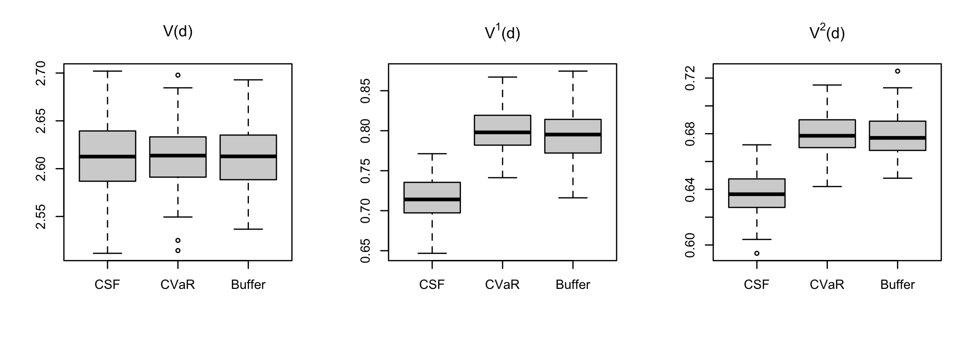
Figure 1: An illustrative example of three criteria

The major contributions of this paper are threefold. First, we propose two robust criteria for learning optimal treatment rules with censored survival data. The first CVaR criterion aims to maximize quantile restricted mean survival time given a pre-specified quantile, where the quantile can be viewed as a quality-adjusted survival time determined by survival function, while the second buffered criterion maximizes survival function at a quality-adjusted survival time, where the quality-adjusted survival time is in turn determined by restricted mean survival time. In particular, we establish a formal link between optimizing restricted mean survival time and optimizing survival probabilities over a class of treatment rules in Lemma 2.1 by effectively leveraging the intrinsic connection between CVaR and bPOE. Second, by leveraging the optimization formulas of CVaR and bPOE and the DC approximation of the indicator function of treatment rules, we construct the difference-of-convex optimization problem to learn the robust treatment rules. We propose a new sampling-based difference-of-convex algorithm with the subsequential convergence to the directional stationary solution, which is applicable to learning treatment rules under both CVaR and bPOE criteria. Third, we develop inverse probability-weighting estimators for both CVaR and bPOE criteria to handle censoring. Under certain regularity conditions, the estimated rule is proved to have a nearly optimal performance in terms of the value function.

The remainder of the article is organized as follows. In Section 2, we present the mathematical framework for individualized treatment rules for right-censored survival outcomes. In Section 3, we propose the theoretical justification of the proposed treatment rules. Extensive simulation studies are presented in Section 5. Numerical studies demonstrate that the proposed method outperforms existing alternatives under the proposed criterion in a variety of settings. We also illustrate our method using a randomized clinical trial in Section 6. The article concludes with a discussion of future work in Section 7. Some needed technical results are provided in the Appendix.

2 Methodology

Suppose we observe a set of $n$ independent and identically distributed (i.i.d.) copies $\{X_{i},A_{i},Y_{i}=(T_{i}\wedge C_{i}),\Delta_{i}=I\{T_{i}\leq C_{i}\},i=1,\ldots,n\}$, where each $X_{i}\in{\mathcal{X}}$ is a $p$-dimensional covariate, $A_{i}\in\{1,-1\}$ is the treatment label, $T_{i}$ is the survival time, $C_{i}$ is the censoring time, and $I\{\cdot\}$ denotes an indicator function. Our goal is to learn robust optimal decision rules to extend survival time and maximize survival probability.

We assume that: i) the survival times $\{T_{i}\}$ are bounded from above by $h>0$ almost surely, where $h$ can be viewed as a restriction time in restricted mean survival time; ii) failure and censoring times are conditionally independent given $X_{i}$ and $A_{i}$, i.e., $T_{i}\perp C_{i}\mid X_{i},A_{i}$ (Fleming and Harrington, 2011); iii) the following positivity assumption holds: $\text{pr}(C_{i}<h|X_{i},A_{i})\leq 1-\eta_{C}$ for some $0<\eta_{C}\leq 1$.

In Sections 2.1-2.3, we start with the complete data $\{(X_{i},A_{i},T_{i})\}_{i=1,\ldots,n}$ and introduce the value function framework and our proposed criteria. From Section 2.4 and hereafter, we account for censoring and consider observed dataset $\{(X_{i},A_{i},Y_{i}=(T_{i}\wedge C_{i}),\Delta_{i}=I\{T_{i}\leq C_{i}\})\}_{i=1,\ldots,n}$.

2.1 Setup and original value function framework

Let $T(d)$ be the potential outcome under a hypothetical intervention that assigns treatment according to treatment rule $d$ that assigns treatment value based on the covariate information $X\in\mathcal{X}$; under the consistency assumption, this potential outcome can be equivalently expressed as

$$T\{d(X)\}\equiv T(1)I\{d(X)=1\}+T(-1)I\{d(X)=-1\},$$

where $T(a)$ is a person’s potential outcome under an intervention that sets treatment to value $a$. The mean-optimal treatment rule in a randomized trial is identified from the observed data by the following expression,

$$\bar{d}(X)={\text{sign}}\{\mathbb{E}(T|X,A=1)-\mathbb{E}(T|X,A=-1)\}.$$

As established by Qian and Murphy (2011), under some mild conditions, learning the mean-optimal individualized treatment rule can alternatively be formulated as maximizing the following value function $V(d)$,

$$\bar{d}=\arg\max_{d}V(d)\equiv\arg\max_{d}\mathbb{E}^{d}\left[T\right]=\arg\max_{d}\mathbb{E}\left[\frac{I\{d(X)=A\}T}{\pi(A|X)}\right],$$ (1)

where $\pi(A|X)$ is the propensity score (Rosenbaum and Rubin, 1983) which is known in randomized experiments, and the superscript $d$ denotes the expectation of the distribution of $(X,A,T)$ given that $A=d(X)$, that is, treatments are chosen according to the treatment rule $d$. Zhang et al. (2012b) proposed to directly maximize the value function over a restricted set of functions.

Rather than maximizing the above value function, Zhao et al. (2012); Zhang et al. (2012a) transformed the above problem into an equivalent weighted classification problem,

$$\bar{d}=\arg\min_{d}\mathbb{E}\left[\frac{T}{\pi(A|X)}I\{d(X)\neq A\}\right],$$ (2)

with 0-1 loss function and weight ${T}/{\pi(A|X)}$. A derivation of Equations (1) and (2) is provided in the Appendix for the purpose of completeness. Zhao et al. (2012) addressed the computational burden of formulation (2) by substituting the zero-one loss with the hinge loss and proposed to solve the optimization via support vector machines. The ensuing classification approach was shown to have appealing robustness properties, particularly in the context of a randomized study where no model assumption on the outcome is needed. In the case of right-censoring, this minimization can be achieved by using plug-in estimators (Zhao et al., 2015b; Cui et al., 2017).

2.2 The CVaR criterion: maximizing restricted mean survival time at a given quantile

In survival analysis, the expected life expectancy within a time window is of great interest (Zhao et al., 2016). Having a good understanding of the area under the survival curve, the celebrated restricted mean survival time (Tian et al., 2014) is easy to present graphically; and moreover, it can be accurately estimated as a functional of the survival function (Zhao and Tsiatis, 1997). However, the choice of truncation, e.g., determining a 5-year or 10-year mark, might sometimes be ad-hoc. In this section, we propose a criterion aiming to maximize the restricted mean survival time, where the restriction time is specified through the quantile of $T(d)$ rather than a fixed truncation because the quantile level is a more interpretable measure. Specifically, we define a new value function for $\gamma\in(0,1)$ as follows,

$$V_{\gamma}^{1}(d)=\mathbb{E}^{d}[TI\{T\leq Q_{\gamma}\{T(d)\}\}],$$ (3)

where $Q_{\gamma}\{Z\}=\inf\{\alpha:\text{pr}(Z\leq\alpha)>\gamma\}$ which is the right $\gamma$-quantile of a random variable $Z$ representing the gains. While Equation (3) has the same form as that in Qi et al. (2019c), our object $T$ here is the restricted survival time. In addition, similar to the property of the restricted mean survival time, Equation (3) enjoys the interpretation of the area under the survival function up to the $\gamma$-quantile. Furthermore, Equation (3) can be connected with the CVaR as follows. Based on the definition of $\mbox{CVaR}_{\gamma}(Z)$ for a random variable $Z$ with the cumulative distribution function $F(\cdot)$ and its optimization formula that $\mbox{CVaR}_{\gamma}(Z)\equiv\frac{1}{1-\gamma}\int_{x\geq\textrm{VaR}_{\gamma}(Z)}x\,\textrm{d}F(x)=\inf_{\alpha\in\mathbb{R}}\{\alpha+\frac{1}{1-\gamma}\mathbb{E}[Z-\alpha]_{+}\}$ for $\gamma\in(0,1)$ given in Rockafellar and Uryasev (2000), we can obtain that

$$\begin{array}[]{ll}V^{1}_{\gamma}(d)&=\mathbb{E}^{d}\,[\,TI\{T\leq Q_{\gamma}\{T(d)\}\}\,]\,=\,\mathbb{E}^{d}\,[\,TI\{-T\geq VaR_{1-\gamma}(-T{(d)})\}\,]\\ &=-\gamma\,\mbox{CVaR}_{1-\gamma}(-T(d))=\gamma\,\sup_{\alpha\in\mathbb{R}}\left\{\alpha-\displaystyle{\frac{1}{\gamma}}\mathbb{E}[(\alpha-T(d))\,I\{T(d)\leq\alpha\}]\right\},\end{array}$$ (4)

which is an unscaled version of decision-rule based CVaR (Rockafellar and Uryasev, 2000) given in Qi et al. (2019c). It is straightforward to see that Equation (4) can be further reformulated as

$$V^{1}_{\gamma}(d)=\sup_{\alpha\in\mathbb{R}}\left\{\alpha\gamma-\mathbb{E}\left[\frac{I\{A=d(X)\}}{\pi(A|X)}(\alpha-T)I(T<\alpha)\right]\right\}.$$ (5)

Thus, with such a connection with CVaR, we refer to it as the CVaR criterion that aims to maximize the restricted mean survival time $V_{\gamma}^{1}(d)$ given a pre-specified survival probability. Next, we propose another criterion, which maximizes the survival probability at a quality-adjusted survival time, where the quality-adjusted survival time is, in turn, determined by restricted mean survival time. In practice, we recommend users choose a criterion based on their goal.

2.3 The buffered criterion: maximizing buffered survival probabilities

For survival time, a survival probability might sometimes be more interpretable for clinicians and patients. In practical uses, one may resort to maximizing the survival function, namely the probability of the survival time exceeding a quality-adjusted survival time (Gelber et al., 1989), where the quality-adjusted survival time can be in turn determined by restricted mean survival time.

For this purpose, we propose the following buffered criterion which aims to maximize the survival function at a quality adjusted survival time that is defined through the restricted mean survival time. We define a new value function $V^{2}_{\tau}(d)$ as follows,

$$V^{2}_{\tau}(d)\equiv\begin{cases}1-\gamma,\,\,\mbox{ with }\gamma\mbox{ satisfying }\frac{V_{\gamma}^{1}(d)}{\gamma}=\tau&\mbox{ for }\tau\in(\inf(T(d)),\mathbb{E}[T(d)]\,]\\ 0&\mbox{ for }\tau>\mathbb{E}[T(d)]\\ 1&\mbox{ for }\tau\leq\inf(T(d))\end{cases}$$ (6)

Such definition is proper because $\frac{V_{\gamma}^{1}(d)}{\gamma}=-\mbox{CVaR}_{1-\gamma}(-T(d))$, which is a continuous and strictly increasing function with respect to $\gamma$ for $\gamma\in(0,1)$ with the range $(\inf(T(d)),\mathbb{E}[T(d)]\,)$.

Remark 1.

When the survival time $T(d)$ is a continuous random variable, the value function is reduced to $V^{2}_{\tau}(d)=\text{pr}(T>q(d))$ with $q(d)$ satisfying $\mathbb{E}[T\,|\,T\leq q(d)]=\tau$. Different from the previous section, Equation (6) enjoys the interpretation of the survival function at the given time point $q(d)$.

We refer to the above criterion as a buffered criterion because it has an interesting connection with bPOE (Rockafellar and Royset, 2010). From a probabilistic perspective, the survival function is known as the probability of exceedance (POE) as a measure of reliability and seems appealing due to its straightforward interpretation. However, the POE disregards the scale of the outcome at tail probability, and thus, a criterion that directly maximizes the survival function may lead to treatment rules that take arbitrarily bad outcomes with a substantial probability. Moreover, the optimization of POE may encounter significant computational difficulties in practice as the POE of a random function is not continuously differentiable or even discontinuous in many situations, particularly when there are only finite scenarios. The theoretical and computational challenges of POE are discussed in detail in Rockafellar and Royset (2010). To overcome those difficulties, bPOE is proposed in Rockafellar and Royset (2010) as an alternative measure of reliability, which provides a conservative upper bound of POE with significant computational advantages.

In the following lemma, we formally link the proposed framework to the concept of bPOE (Mafusalov and Uryasev, 2018), so that we can effectively leverage Proposition 2.2 of Mafusalov and Uryasev (2018) to solve our optimization problem in mind.

Lemma 2.1.

For the value function defined in (6), with $\tau\in(\inf(T(d)),\mathbb{E}[T(d)]\,]$ we have

$$V^{2}_{\tau}(d)=1-\inf_{c\geq 0}\mathbb{E}^{d}[\max(0,c(-T+\tau)+1)].$$

Therefore, maximizing $V_{\tau}^{2}(d)$ over $d$ is equivalent to $\mbox{minimize }M^{2}_{\tau}(d)$ over $d$ with

$$M^{2}_{\tau}(d)\equiv\inf_{c\geq 0}\,\mathbb{E}^{d}\left[\max(0,c(-T+\tau)+1)\right].$$

Proof.

Notice that based on the definition of bPOE in (Mafusalov and Uryasev, 2018, Definition 2.1),

$$\begin{array}[]{ll}\min\{\gamma:-\mbox{CVaR}_{1-\gamma}(-T(d))\geq\tau\}=1-\max\{\gamma:\mbox{CVaR}_{\gamma}(-T(d))\leq-\tau\}=\mbox{bPOE}(-T(d);-\tau).\end{array}$$

Thus, by Proposition 2.2 in Mafusalov and Uryasev (2018) that

$$\mbox{bPOE}(T;\tau)=\inf_{c\geq 0}\mathbb{E}\left[\max(0,c(T-\tau)+1)\right],$$

we have $V^{2}_{\tau}(d)=1-\inf_{c\geq 0}\mathbb{E}^{d}[\max(0,c(-T+\tau)+1)]$. Thus, the maximization of $V_{\tau}^{2}(d)$ over $d$ is equivalent to $\min_{d}\,\inf_{c\geq 0}\mathbb{E}^{d}\left[\max(0,c(-T+\tau)+1)\right].$

∎

2.4 Accounting for censoring

Hereafter, to streamline the presentation, we write $V^{1}_{\gamma}(d)$ and $M^{2}_{\tau}(d)$ as $V^{1}(d)$ and $M^{2}(d)$, respectively. As $T$ is only partially observed, by leveraging the following lemma, we can express $V^{1}(d)$ and $M^{2}(d)$ in terms of the observed right-censored data $Y=(T\wedge C)$.

Lemma 2.2.

With $\Delta\equiv I(T\leq C)$, and $S_{C}(\cdot|X,A)$ denoting the conditional survival function of the censoring distribution, we have

$$V^{1}(d) =\sup_{\alpha\in\mathbb{R}}\left\{\alpha\gamma-\mathbb{E}\left[\frac{\Delta(\alpha-Y)I(\alpha\geq Y)}{S_{C}(Y|X,A)}\frac{I\{A=d(X)\}}{\pi(A|X)}\right]\right\},$$

$$M^{2}(d) =\inf_{c\geq 0}\left\{\mathbb{E}\left[\frac{\Delta\max(0,c(-Y+\tau)+1)}{S_{C}(Y|X,A)}\frac{I\{A=d(X)\}}{\pi(A|X)}\right]\right\}.$$

Proof.

For the first criterion, recall that $V^{1}(d)=\sup_{\alpha\in\mathbb{R}}\left\{\alpha\gamma-\mathbb{E}\left[(\alpha-T)I(T\leq\alpha)\frac{I\{A=d(X)\}}{\pi(A|X)}\right]\right\}.$ Note that

$$\mathbb{E}\left[(\alpha-T)I(T\leq\alpha)\frac{I\{A=d(X)\}}{\pi(A|X)}\right]$$

$$= \mathbb{E}\left\{\mathbb{E}\big{[}(\alpha-T)I(T\leq\alpha)|X,A\big{]}\,\mathbb{E}\left[\frac{I\{A=d(X)\}}{\pi(A|X)}\Big{|}X,A\right]\right\}$$

$$= \mathbb{E}\left\{\mathbb{E}\left[\frac{(\alpha-T)I(T\leq C)I(T\leq\alpha)}{\text{pr}(C\geq T|X,A)}\Big{|}X,A\right]\,\mathbb{E}\left[\frac{I\{A=d(X)\}}{\pi(A|X)}\Big{|}X,A\right]\right\}$$

$$= \mathbb{E}\left\{\mathbb{E}\left[\frac{\Delta(\alpha-Y)I(\alpha\geq Y)}{\text{pr}(C\geq Y|X,A)}\Big{|}X,A\right]\mathbb{E}\left[\frac{I\{A=d(X)\}}{\pi(A|X)}\Big{|}X,A\right]\right\}.$$

It further equals to $\mathbb{E}\left[\frac{\Delta(\alpha-Y)I(\alpha\geq Y)}{\text{pr}(C\geq Y|X,A)}\frac{I\{A=d(X)\}}{\pi(A|X)}\right]$ which completes our proof.

For the second criterion, recall that $M^{2}(d)=\inf_{c\geq 0}\mathbb{E}^{d}\left[\max(0,c(-T+\tau)+1)\right]$. Then

$$\mathbb{E}\left[\max(0,c(-T+\tau)+1)\frac{I\{A=d(X)\}}{\pi(A|X)}\right]$$

$$= \mathbb{E}\left\{\mathbb{E}\big{[}\max(0,c(-T+\tau)+1)|X,A\big{]}\,\mathbb{E}\left[\frac{I\{A=d(X)\}}{\pi(A|X)}\Big{|}X,A\right]\right\}$$

$$= \mathbb{E}\left\{\mathbb{E}\left[\frac{\max(0,c(-T+\tau)+1)I(T\leq C)}{\text{pr}(C\geq T|X,A)}\Big{|}X,A\right]\mathbb{E}\left[\frac{I\{A=d(X)\}}{\pi(A|X)}\Big{|}X,A\right]\right\}$$

$$= \mathbb{E}\left\{\mathbb{E}\left[\frac{\Delta\max(0,c(-Y+\tau)+1)}{\text{pr}(C\geq Y|X,A)}\Big{|}X,A\right]\mathbb{E}\left[\frac{I\{A=d(X)\}}{\pi(A|X)}\Big{|}X,A\right]\right\}.$$

It further equals to $\mathbb{E}\left[\frac{\Delta\max(0,c(-Y+\tau)+1)}{\text{pr}(C\geq Y|X,A)}\frac{I\{A=d(X)\}}{\pi(A|X)}\right]$, which completes our proof. ∎

Lemma 2.2 provides the explicit formulation of the two robust criteria with censored data. However, the conditional survival function $S_{C}(Y|X,A)$ of the censoring distribution is generally unknown in practice. Moreover, the discontinuous indicator function appearing in $V^{1}(d)$ and $M^{2}(d)$ leads to the significant computational difficulties in learning the treatment rules. Therefore, we propose the estimated treatment regimes under the two aforementioned robust criteria to resolve the two aforementioned difficulties. First, the conditional survival function $S_{C}(Y|X,A)$ can be estimated by Cox proportional hazards models (Cox, 1972) or random survival forests (Ishwaran et al., 2008) $\widehat{S}_{C}(Y|X,A)$ based on historical data which can be then plugged into the two robust criteria. Regarding to the indicator function, by writing $d(X)={\text{sign}}(f(X))$ where $f(\bullet)$ is chosen from a hypothesis class $\mathcal{H}$, an implementable approach is to approximate the indicator function $I(A={\text{sign}}(f(X)))=I(A\,f(X)>0)$ by continuous surrogate functions. For instance, a smooth difference-of-convex function is constructed in Qi et al. (2019c) as the surrogate function of the indicator function $I(t>0)$. For such an indicator function, we assume the existence of a surrogate function $\mathcal{L}(t)$ with the DC representation $\mathcal{L}(t)\equiv\mathcal{L}_{1}(t)-\mathcal{L}_{2}(t)\geq 0$, where $\mathcal{L}_{1}$ and $\mathcal{L}_{2}$ are differentiable convex functions. For example,

$${\mathcal{L}}(u)=\begin{cases}0&\text{if $u<-\delta$},\\ \frac{1}{2}(1+u/\delta)^{2}&\text{if $0>u\geq-\delta$},\\ 1-\frac{1}{2}(1-u/\delta)^{2}&\text{if $\delta>u\geq 0$},\\ 1&\text{if $u>\delta$},\end{cases}$$

and

$${\mathcal{L}}_{1}(u)=\begin{cases}0&\text{if $u\leq-\delta$},\\ \frac{1}{2}(1+u/\delta)^{2}&\text{if $-\delta<u\leq 0$},\\ \frac{1}{2}+u/\delta&\text{if $u>0$},\end{cases}~{}~{}{\mathcal{L}}_{2}(u)=\begin{cases}0&\text{if $u\leq 0$},\\ \frac{1}{2}(u/\delta)^{2}&\text{if $0<u\leq\delta$},\\ u/\delta-\frac{1}{2}&\text{if $u>\delta$}.\end{cases}$$

Then, we obtain the estimated treatment regimes under the two robust criteria as follows,

$$\mbox{maximize}_{f\in\mathcal{H}}\quad V^{\wedge}_{\mathcal{L}}(f) \equiv\sup_{\alpha}\left\{\mathbb{E}\left[\left(\alpha\gamma-\frac{\Delta(\alpha-Y)I(\alpha\geq Y)}{\widehat{S}_{C}(Y|X,A)}\right)\frac{{\mathcal{L}}(Af(X))}{\pi(A|X)}\right]\right\},$$ (7)

$$\mbox{minimize}_{f\in\mathcal{H}}\quad M^{\wedge}_{\mathcal{L}}(f) \equiv\inf_{c\geq 0}\left\{\mathbb{E}\left[\frac{\Delta\max(0,c(-Y+\tau)+1)}{\widehat{S}_{C}(Y|X,A)}\frac{\mathcal{L}(Af(X))}{\pi(A|X)}\right]\right\}.$$ (8)

3 Asymptotic properties

In this section, we provide the asymptotic results of the proposed estimated treatment regimes (7) and (8). The purpose of this section is to demonstrate that the value function of the estimated optimal treatment regime converges to the optimal value function under the CVaR and buffered criteria, respectively. In particular, we establish Fisher consistency, excess risk bound, and universal consistency of the estimated optimal treatment regimes.

We start with introducing some notations for the CVaR criterion. Recall that according to Lemma 2.2,

$$V^{1}(d) =\sup_{\alpha\in\mathbb{R}}\left\{\mathbb{E}\left[\left\{\alpha\gamma-\frac{\Delta(\alpha-Y)I(\alpha\geq Y)}{S_{C}(Y|X,A)}\right\}\frac{I\{A=d(X)\}}{\pi(A|X)}\right]\right\},$$

With $d(X)=\mbox{sign}(f(X))$ and the surrogate function $\mathcal{L}$ of the indicator function, we define

$$V^{1}_{\mathcal{L}}(f,\alpha)\equiv \mathbb{E}\left[\left\{\alpha\gamma-\frac{\Delta(\alpha-Y)I(\alpha\geq Y)}{S_{C}(Y|X,A)}\right\}\frac{{\mathcal{L}}(Af(X))}{\pi(A|X)}\right],$$

as the surrogate value function. We define the value function and surrogate value function corresponding to the working model as

$$V^{\wedge,1}(d,\alpha) \equiv\mathbb{E}\left[\left\{\alpha\gamma-\frac{\Delta(\alpha-Y)I(\alpha\geq Y)}{\widehat{S}_{C}(Y|X,A)}\right\}\frac{I\{A=d(X)\}}{\pi(A|X)}\right],$$

$$V^{\wedge,1}_{\mathcal{L}}(f,\alpha) \equiv\mathbb{E}\left[\left\{\alpha\gamma-\frac{\Delta(\alpha-Y)I(\alpha\geq Y)}{\widehat{S}_{C}(Y|X,A)}\right\}\frac{{\mathcal{L}}(Af(X))}{\pi(A|X)}\right],$$

respectively, where $\mathbb{E}$ is taken with respect to $(Y,\Delta,A,X)$ conditional on $\widehat{S}_{C}$. We also define

$$V^{\prime,1}(d,\alpha) \equiv\mathbb{E}\left[\left\{\alpha\gamma-\frac{\Delta(\alpha-Y)I(\alpha\geq Y)}{\widetilde{S}_{C}(Y|X,A)}\right\}\frac{I\{A=d(X)\}}{\pi(A|X)}\right],$$

$$V^{\prime,1}_{\mathcal{L}}(f,\alpha) \equiv\mathbb{E}\left[\left\{\alpha\gamma-\frac{\Delta(\alpha-Y)I(\alpha\geq Y)}{\widetilde{S}_{C}(Y|X,A)}\right\}\frac{{\mathcal{L}}(Af(X))}{\pi(A|X)}\right],$$

where $\widetilde{S}_{C}(\cdot|X,A)$ is the probability limit of $\widehat{S}_{C}(\cdot|X,A)$. We denote $(\widetilde{f},\widetilde{\alpha})\in\underset{f\in{\cal H},\alpha\in\mathbb{R}}{\mathop{\mathrm{argmax}}}V^{\prime,1}_{\mathcal{L}}(f,\alpha)$.

We first establish Fisher consistency of estimating optimal treatment rules under $V^{\prime,1}_{\mathcal{L}}(f,\alpha)$ to justify the use of the surrogate loss ${\mathcal{L}}(u)$. Based on Theorem 3.1, it is equivalent to considering $V^{\prime,1}_{\mathcal{L}}(f,\alpha)$ rather than $V^{\prime,1}(d,\alpha)$.

Theorem 3.1.

If $(\widetilde{f},\widetilde{\alpha})$ maximizes $V^{\prime,1}_{\mathcal{L}}(f,\alpha)$, then $({\text{sign}}(\widetilde{f}),\widetilde{\alpha})$ maximizes $V^{\prime,1}(d,\alpha)$.

We then establish the consistency of the estimated treatment rule with a universal kernel, e.g., the functional class ${\cal H}$ is RKHS endowed by a Gaussian kernel. Estimation error has two potential sources, the first of which is uncertainty in the estimated conditional survival functions, and the second is from the estimation of the optimal treatment rules.

As an intermediate step for the consistency proof, we then establish the following excess risk of the estimated treatment rule:

Theorem 3.2.

For any measurable function $f$ and $\alpha\in\mathbbm{R}$,

$$\sup_{f^{\prime}\in{\mathcal{F}},\alpha^{\prime}\in\mathbb{R}}V^{\prime,1}({\text{sign}}(f^{\prime}),\alpha^{\prime})-V^{\prime,1}({\text{sign}}(f),\alpha)\leq V^{\prime,1}_{\mathcal{L}}(\widetilde{f},\widetilde{\alpha})-V^{\prime,1}_{\mathcal{L}}(f,\alpha).$$

By leveraging Theorem 3.2, we establish the consistency of the estimated treatment rule:

Theorem 3.3.

Suppose that $\sup_{x\in\mathcal{{\mathcal{X}}},t\leq h}|\widehat{S}_{C}(t|x,a)-S_{C}(t|x,a)|\overset{p}{\to}0$ for both $a=-1,1$, then we have the following convergence in probability,

$$\lim_{n\rightarrow\infty}\sup_{\alpha\in\mathbb{R}}V^{1}({\text{sign}}(\widehat{f}\,),{\alpha})=V^{1}({\text{sign}}(f^{\star}),\alpha^{\star}),$$

where $(f^{\star},\alpha^{\star})$ is defined as $(f^{\star},\alpha^{\star})\in\underset{\alpha\in\mathbb{R},f\in{\cal H}}{\arg\max}\,V^{1}({\text{sign}}(f),\alpha)$, and $(\widehat{f},\widehat{\alpha})$ solves the empirical optimization problem (9).

The assumption on $\widehat{S}_{C}(t|x,a)$ is quite general. In particular, the consistency with certain rates can be achieved by parametric models as wells as nonparametric methods such as survival forests (Cui et al., 2022) and nonparametric kernel smoothing methods (Sun et al., 2019). The rate of convergence of the estimated treatment rule can be studied under certain standard assumptions in the learning theory literature (Steinwart and Christmann, 2008), and we omit here.

Analogously, for the buffered criterion, we define

$$V^{2}(d,c) \equiv\mathbb{E}\left[-\left\{\frac{\Delta\max(0,c(-Y+\tau)+1)}{S_{C}(Y|X,A)}\right\}\frac{I\{A=d(X)\}}{\pi(A|X)}\right],$$

$$V^{2}_{\mathcal{L}}(f,c) \equiv\mathbb{E}\left[-\left\{\frac{\Delta\max(0,c(-Y+\tau)+1)}{S_{C}(Y|X,A)}\right\}\frac{{\mathcal{L}}(Af(X))}{\pi(A|X)}\right],$$

$$V^{\wedge,2}(d,c) \equiv\mathbb{E}\left[-\left\{\frac{\Delta\max(0,c(-Y+\tau)+1)}{\widehat{S}_{C}(Y|X,A)}\right\}\frac{I\{A=d(X)\}}{\pi(A|X)}\right],$$

$$V^{\wedge,2}_{\mathcal{L}}(f,c) \equiv\mathbb{E}\left[-\left\{\frac{\Delta\max(0,c(-Y+\tau)+1)}{\widehat{S}_{C}(Y|X,A)}\right\}\frac{{\mathcal{L}}(Af(X))}{\pi(A|X)}\right],$$

$$V^{\prime,2}(d,c) \equiv\mathbb{E}\left[-\left\{\frac{\Delta\max(0,c(-Y+\tau)+1)}{\widetilde{S}_{C}(Y|X,A)}\right\}\frac{I\{A=d(X)\}}{\pi(A|X)}\right],$$

$$V^{\prime,2}_{\mathcal{L}}(f,c) \equiv\mathbb{E}\left[-\left\{\frac{\Delta\max(0,c(-Y+\tau)+1)}{\widetilde{S}_{C}(Y|X,A)}\right\}\frac{{\mathcal{L}}(Af(X))}{\pi(A|X)}\right],$$

and $(\widetilde{f},\widetilde{c})\in\mathop{\mathrm{argmax}}_{f\in{\cal H},c\geq 0}V^{\prime,2}_{\mathcal{L}}(f,c)$.

We then have the following theorems for the buffered criterion.

Theorem 3.4.

If $(\widetilde{f},\widetilde{c})$ maximizes $V^{\prime,2}_{\mathcal{L}}(f,c)$, then $({\text{sign}}(\widetilde{f}),\widetilde{c})$ maximizes $V^{\prime,2}(d,c)$.

Theorem 3.5.

For any measurable function $f$ and $c\geq 0$,

$$\sup_{f\in{\cal H},c\geq 0}V^{\prime,2}({\text{sign}}(f),c)-V^{\prime,2}({\text{sign}}(f),c)\leq V^{\prime,2}_{\mathcal{L}}(\widetilde{f},\widetilde{c})-V^{\prime,2}_{\mathcal{L}}(f,c).$$

Theorem 3.6.

Suppose $\sup_{x\in\mathcal{{\mathcal{X}}},t\leq\tau}|\widehat{S}_{C}(t|x,a)-S_{C}(t|x,a)|\overset{p}{\to}0$ for both $a=-1,1$, then we have the following convergence in probability,

$$\lim_{n\rightarrow\infty}\sup_{c\geq 0}V^{2}({\text{sign}}(\widehat{f}),{c})=V^{2}({\text{sign}}(f^{\star}),c^{\star}),$$

where $(f^{\star},c^{\star})$ is defined as $(f^{\star},c^{\star})\in\underset{c\geq 0,f\in{\cal H}}{\arg\max}\,V^{2}({\text{sign}}(f),c)$, and $(\widehat{f},\widehat{c})$ solves the empirical optimization problem (10).

The proofs for all theorems are deferred to the Appendix.

4 Sampling-based algorithm for learning the treatment rules

In this section, we focus on the algorithmic development for learning the treatment rules with censored data under the two robust criteria with observed data $Z_{i}\equiv(X_{i},A_{i},Y_{i},\Delta_{i})$ for ${i=1,\ldots,n}$. We make two assumptions below.

(A1) the surrogate function $\mathcal{L}(\bullet)$ satisfies that $\mathcal{L}(t)\in[0,1]$ for every $t\in\mathbb{R}$, and $\mathcal{L}(\bullet)=\mathcal{L}_{1}(\bullet)-\mathcal{L}_{2}(\bullet)$ where $\mathcal{L}_{1}(\bullet)$ and $\mathcal{L}_{2}(\bullet)$ are smooth convex functions with the Lipschitz gradient modulus $L$;

(A2) $\mathcal{H}$ is a Reproducing Kernel Hilbert Space (RKHS) with the norm $\|\bullet\|_{\mathcal{H}}$ and the corresponding real-valued kernel $k:{\mathcal{X}}\times{\mathcal{X}}\to\mathbb{R}$ that is symmetric and positive-definite.

For treatment learning tasks under the two robust criteria, we can formulate the corresponding empirical problems with a regularization as follows:

$$\underset{f\in{\mathcal{H}}}{\mbox{maximize}}\quad\left(\sup_{\alpha\in\mathbb{R}}\,\,\alpha\gamma-\frac{1}{n}\sum_{i=1}^{n}\frac{\mathcal{L}(A_{i}\,K_{i}^{\top}\beta)}{\pi(A_{i}|X_{i})}\frac{\Delta_{i}(\alpha-Y_{i})I(Y_{i}\leq\alpha)}{\widehat{S}_{C}(Y_{i}|X_{i},A_{i})}+\lambda\|f\|_{\mathcal{H}}^{2}\right),$$ (9)

$$\underset{f\in{\mathcal{H}}}{\mbox{minimize}}\quad\left(\inf_{c\geq 0}\,\,\frac{1}{n}\sum_{i=1}^{n}\frac{\mathcal{L}(A_{i}\,K_{i}^{\top}\beta)}{\pi(A_{i}|X_{i})}\left\{\frac{\Delta_{i}\max(0,c(-Y_{i}+\tau)+1)}{\widehat{S}_{C}(Y_{i}|X_{i},A_{i})}\right\}+\lambda\|f\|_{\mathcal{H}}^{2}\right).$$ (10)

Hereinafter, under the above two assumptions we focus on solving Problem (9) and we will show later that the proposed algorithm can be applied to solve Problem (10) as well. By the Representer theorem, with $W_{i}\equiv\frac{\Delta_{i}}{\pi(A_{i}\mid X_{i})\,\widehat{S}_{C}(Y_{i}|X_{i},A_{i})}$, $K_{ij}\equiv k(X_{i},X_{j})$, Problem (9) can be reformulated as follows,

$$\underset{\beta\in\mathbb{R}^{n}}{\mbox{minimize}}\quad\left(V(\beta)\equiv\underset{\alpha\in\mathbb{R}}{\inf}\,-\frac{1}{n}\sum_{i=1}^{n}\,{\psi}(\beta,\alpha;Z_{i})+\lambda\,\beta^{\top}K\beta\right)$$ (11)

where $\psi(\beta,\alpha;Z_{i})\equiv\alpha\,\gamma-\left(\,\mathcal{L}_{1}\big{(}A_{i}\,K_{i}^{\top}\beta\big{)}-\mathcal{L}_{2}\big{(}A_{i}\,K_{i}^{\top}\beta\big{)}\,\right)\,W_{i}\,(\alpha-Y_{i})_{+}$. To simplify the notation, we omit the superscript for $V$. According to Rockafellar and Uryasev (2000), the optimal solution of $\alpha$ in (11) should be contained in a bounded set. Moreover, since ${\psi}(f,\bullet;Z_{i})$ is a concave piecewise affine function with knots $\{Y_{i}\}_{i=1}^{n}$, it is shown in Qi et al. (2019c) that the inner minimization over $\alpha$ in (11) achieves its optimum at one of the knots $\{Y_{i}\}_{i=1}^{n}$. Thus, the objective function of (11) can be rewritten as

$$\begin{array}[]{lll}V(\beta)=\underset{j\in[n]}{\mbox{min}}\,-\displaystyle{\frac{1}{n}\sum_{i=1}^{n}}\,{\psi}(\beta,Y_{j};Z_{i})+\lambda\,\beta^{\top}K\beta,\end{array}$$

and with $\overline{Y}_{i}\equiv\sum_{k=1}^{n}\,(Y_{k}-Y_{i})_{+}$, $\widehat{Y}_{i,j}\equiv\sum_{k(\neq j)=1}^{n}\,(Y_{k}-Y_{i})_{+}$, it can further be decomposed into the difference of two convex functions as follows:

$$\begin{array}[]{lll}V(\beta)&=&\underset{j\in[n]}{\mbox{min}}\quad-\displaystyle{\frac{1}{n}}\sum_{i=1}^{n}\Big{(}Y_{j}\,\gamma-\big{(}\,\mathcal{L}_{1}(A_{i}\,K_{i}^{\top}\beta)-\mathcal{L}_{2}(A_{i}\,K_{i}^{\top}\beta)\,\big{)}(Y_{j}-Y_{i})_{+}W_{i}\Big{)}+\lambda\,\beta^{\top}K\beta\\[7.22743pt] &=&\underbrace{\displaystyle{\frac{1}{n}}\sum_{i=1}^{n}\,\mathcal{L}_{1}(A_{i}\,K_{i}^{\top}\beta)\,\overline{Y}_{i}W_{i}}_{\mbox{denoted by }\varphi_{1}(\beta)}+\lambda\,\beta^{\top}K\beta\\[36.135pt] &&-\,\underset{j\in[n]}{\mbox{max}}\,\underbrace{\displaystyle{\frac{1}{n}}\sum_{i=1}^{n}\left(\,Y_{j}\,\gamma+\displaystyle{{\mathcal{L}_{1}(A_{i}\,\,K_{i}^{\top}\beta)}}\,\widehat{Y}_{i,j}\,W_{i}+\mathcal{L}_{2}(A_{i}\,\,K_{i}^{\top}\beta)(Y_{j}-Y_{i})_{+}W_{i}\right)\,}_{\mbox{denoted by }\varphi_{2,j}(\beta)}.\end{array}$$ (12)

The optimization problem (11) is a DC program, and as implemented in Qi et al. (2019c) the deterministic DC algorithms and its enhanced variation proposed by Pang et al. (2016) can be applied for obtaining a critical or d-stationary solutions. However, due to the finite-sum structures of the two convex component functions in (12), DC algorithms need to iteratively solve convex subproblems with finite-sum over the whole data set, and thus could be highly computational inefficient especially when the data size $n$ is large. Therefore, we propose a sampling-based DC algorithm for solving Problem (11). Specifically, with a sample set $\{Z_{i}:i\in I_{\nu}\}$ of size $N_{\nu}$ i.i.d. generated from the whole data set $\{Z_{i}\}_{i=1}^{n}$, we can first construct a sampling-based approximation function:

$$\begin{array}[]{lll}\widetilde{V}^{(\nu)}(\beta)&\equiv&\underset{j\in\mathcal{I}_{\nu}}{\mbox{min}}\,-\displaystyle{\frac{1}{N_{\nu}}}\sum_{i\in I_{\nu}}\,{\psi}(\beta,Y_{j};Z_{i})+\lambda\,\beta^{\top}K\beta\\[21.68121pt] &=&\underbrace{\displaystyle{\frac{1}{N_{\nu}}}\sum_{i\in I_{\nu}}\,\mathcal{L}_{1}(A_{i}\,K_{i}^{\top}\beta)\,\overline{Y}_{i}^{\nu}\,W_{i}}_{\mbox{denoted by }\tilde{\varphi}_{1}^{(\nu)}(\beta)}+\lambda\,\beta^{\top}K\beta\\[36.135pt] &&-\underset{j\in\mathcal{I}_{\nu}}{\mbox{max}}\quad\underbrace{\displaystyle{\frac{1}{N_{\nu}}}\sum_{i\in I_{\nu}}\left(\,Y_{j}\,\gamma+\displaystyle{{\mathcal{L}_{1}(A_{i}\,\,K_{i}^{\top}\beta)}}\widehat{Y}_{i,j}^{\nu}\,W_{i}+\mathcal{L}_{2}(A_{i}\,\,K_{i}^{\top}\beta)(Y_{j}-Y_{i})_{+}W_{i}\right)\,}_{\mbox{denoted by }\tilde{\varphi}^{(\nu)}_{2,j}(\beta)},\end{array}$$

where $\overline{Y}^{(\nu)}_{i}\equiv\sum_{k\in I_{\nu}}\,(Y_{k}-Y_{i})_{+}$, $\widehat{Y}^{(\nu)}_{i,j}\equiv\sum_{k(\neq j)\in I_{\nu}}\,(Y_{k}-Y_{i})_{+}$. Due to the finite min operator, such a sampling-based approximation function $\widetilde{V}^{(\nu)}(\beta)$ is a biased estimator of $V(\beta)$, which necessitates a particular sampling scheme in the follow-up algorithmic development and convergence analysis. With the following active index sets,

$$\begin{array}[]{ll}\mathcal{M}(\beta)\equiv\underset{j\in[n]}{\mbox{argmin}}\,\,\,\ \displaystyle{\frac{1}{n}\sum_{i=1}^{n}}\psi(\beta,Y_{j};Z_{i}),\\[14.45377pt] \widetilde{\mathcal{M}}^{(\nu)}_{\varepsilon}(\beta)\equiv\left\{\ell\in\mathcal{I}_{\nu}:\displaystyle{\frac{1}{N_{\nu}}\sum_{i=1}^{N_{\nu}}}\psi(\beta,Y_{\ell};Z_{i})\leq\min_{j\in\mathcal{I}_{\nu}}\,\displaystyle{\frac{1}{N_{\nu}}\sum_{i=1}^{N_{\nu}}}\psi(\beta,Y_{j};Z_{i})+\varepsilon\right\},\quad\mbox{ with }\varepsilon\geq 0,\end{array}$$

we define the linear approximation functions of ${\varphi}_{2,j}(\beta)$ and $\widetilde{\varphi}_{2,j}^{(\nu)}(\beta)$ respectively at a reference point $\beta^{(\nu)}$:

$$\begin{array}[]{ll}\widehat{\varphi}_{2,j}(\beta;\beta^{(\nu)})\equiv&{\varphi}_{2,j}(\beta^{(\nu)})+\langle\nabla{\varphi}_{2,j}(\beta^{(\nu)}),\,\beta-\beta^{(\nu)}\rangle,\mbox{ for any }j\in\mathcal{M}(\beta),\\[7.22743pt] \widehat{\varphi}_{2,j}^{(\nu)}(\beta;\beta^{(\nu)})\equiv&\widetilde{\varphi}^{(\nu)}_{2,j}(\beta^{(\nu)})+\langle\nabla\widetilde{\varphi}^{(\nu)}_{2,j}(\beta^{(\nu)}),\,\beta-\beta^{(\nu)}\rangle,\mbox{ for any }j\in\widetilde{\mathcal{M}}^{(\nu)}_{\varepsilon}(\beta).\end{array}$$ (13)

Accordingly, we can construct the sampling-based convexified approximation function of $V(\beta)$ as follows, $\widehat{V}^{(\nu)}_{j}(\beta;\beta^{(\nu)})\equiv\widetilde{\varphi}_{1}^{(\nu)}(\beta)-\widehat{\varphi}_{2,j}^{(\nu)}(\beta;\beta^{(\nu)})+\lambda\,\beta^{\top}K\beta$ for every $j\in\widetilde{\mathcal{M}}^{(\nu)}_{\varepsilon}(\beta)$.

We develop a sampling-based algorithm below which is embedded with three sequential steps: sampling, DC-decomposition, and convexification. At iteration $\nu$, with i.i.d. generated sample set $\{Z_{i}:i\in I_{\nu}\}$ containing newly generated samples and all historically generated samples, for every index $j\in\widetilde{M}_{\nu}^{\varepsilon}(\beta)$, we can constitute a sampling-based convexified approximation function $\widehat{V}^{(\nu)}_{j}(\beta;\beta^{(\nu)})$, and further obtain the corresponding proximal mapping point by implementing the convex-programming solver. Due to the finite-max structure of the second component function in DC decomposition (12) together with the biased estimation, we tailor the enhancement technique of deterministic DCA in Pang et al. (2016) for such a sampling-based algorithm; namely in Steps 4 and 5 of the proposed algorithm, we select the best candidate solution over the $\varepsilon$-active index set as the next iterate point. We will show such an enhancement technique yields the convergence to a directional stationary solution that is known as being the sharpest stationarity type for general nonconvex problems.

 

Algorithm 1

 

1:  Initialization: Let $\beta^{(0)}\in\mathbb{R}^{n}$ and positive scalars $\rho,\lambda,\varepsilon$ be given. Set $N_{0}=0$.

2:  for $\nu=1,2,\cdots$, do

3:     generate an independent sample set $\{Z_{i}:i\in K_{\nu}\}$ of size $\Delta_{\nu}$ i.i.d. from the whole sample set $\{Z_{i}\}_{i=1}^{n}$ and set $I_{\nu}\equiv I_{\nu-1}\cup K_{\nu}$, and $N_{\nu}\equiv N_{\nu-1}+\Delta_{\nu}$;

4:     for every $j\in\widetilde{\mathcal{M}}_{\nu}^{\varepsilon}(\beta^{(\nu)})$, compute $\beta^{(\nu+1/2)}_{j}=\underset{\beta\,\in\,\mathbb{R}^{n}}{\mbox{argmin}}\left\{\,\widehat{V}^{(\nu)}_{j}(\beta;\beta^{(\nu)})+\displaystyle{\frac{1}{2\rho}}\,\|\beta-\beta^{(\nu)}\|^{2}\,\,\right\};$

5:     let $j_{\nu}\in\displaystyle{\mbox{argmin}_{j\in\widetilde{\mathcal{M}}_{\nu}^{\varepsilon}(\beta^{(\nu)})}}\,\left\{\widetilde{V}^{(\nu)}(\beta^{(\nu+1/2)}_{j})+\displaystyle{\frac{1}{2\rho}}\,\|\beta^{(\nu+1/2)}_{j}-\beta^{(\nu)}\|^{2}\,\,\right\}$ and set $\beta^{(\nu+1)}=\beta^{(\nu+1/2)}_{j_{\nu}}$

6:  end for

 

It is worth noticing that the proposed sampling-based DC algorithm has several major distinctions from some recent works on sampling-based DC algorithms in Le Thi et al. (2019) and Liu and Pang (2022), which thus necessitates a separate convergence analysis afterwards. First, stochastic DC algorithm of Le Thi et al. (2019) is developed for a class of DC programs where both two convex component functions are expectation functions, whereas DC programs studied in the present paper and in Liu and Pang (2022) both contain the second component functions that are the value function of finite-sum or expectation functions. Second, we construct the sampling-based convexified approximation function with a sequential sampling and DC-decomposition, so that we only use one single sample set for both two convex component functions. Since the two component functions are much likely to have positive covariance due to the shared parts, such a common random number technique leads to solution sequences with less volatility compared to the algorithm in Liu and Pang (2022) with independent sampling strategy for the two component functions. The third distinction is that based on the finite-max structure of (12), we integrate the enhanced technique into the sampling-based DC algorithm in order to obtain the directional stationary solution, which distinguishes the proposed algorithm and the convergence analysis from the sampling-based algorithm in Liu and Pang (2022) which can only achieves the convergence to critical solutions to the stochastic DC value function optimization problem.

Recall that for the minimization of a B(ouligand)-differentiable function $f$ over a convex set $\mathcal{X}^{\prime}$, we say that $\bar{x}$ is a directional stationary solution if $f^{\prime}(\bar{x};x-\bar{x})\equiv\lim_{t\to 0}\frac{f(\bar{x}+t(x-\bar{x}))-f(\bar{x})}{t}\geq 0$ for any $x\in\mathcal{X}^{\prime}$. We present the convergence result of the proposed algorithm with the proof provided in Appendix D.

Theorem 4.1.

Under assumptions (A1) and (A2), with $\Delta_{\nu}\geq C$ for some positive integer $C$, with arbitrary $\rho\geq 0$ and $\lambda>0$, any limit point $\beta^{\,\infty}$ of the sequence $\{\beta^{(\nu)}\}$ generated by Algorithm 1 if exists is a directional stationary point of (11) with probability 1.

For learning the treatment rule under the buffered criterion, by utilizing the DC surrogation of the indicator function, the optimization problem is formulated below.

$$\underset{\beta\in\mathbb{R}^{n}}{\mbox{minimize}}\quad\inf_{c\geq 0}\,\,\frac{1}{n}\sum_{i=1}^{n}\left(\mathcal{L}_{1}(A_{i}\,K_{i}^{\top}\beta)-\mathcal{L}_{2}(A_{i}\,K_{i}^{\top}\beta)\right)\max(0,c(-Y_{i}+\tau)+1)W_{i},$$

Similar to case of the CVaR criterion, the inner minimization over $c$ also achieves the optimum at one of the knots $\{\frac{1}{Y_{i}-\tau}\}_{i=1}^{n}$. Hence, the optimization problem can be written as

$$\underset{\beta\in\mathbb{R}^{n}}{\mbox{minimize}}\quad M(\beta)\triangleq\min_{j\in[n]}\,\frac{1}{n}\sum_{i=1}^{n}\left(\mathcal{L}_{1}(A_{i}\,K_{i}^{\top}\beta)-\mathcal{L}_{2}(A_{i}\,K_{i}^{\top}\beta)\right)\max\left\{0,\frac{(-Y_{i}+\tau)+1}{Y_{j}-\tau}\right\}W_{i},$$ (14)

The objective function $M(\beta)$ is the minimization of finite sum of DC functions, and thus has the similar DC decomposition as in (12) under the CVaR criterion. Hence for learning the treatment rule under the buffered criterion, we can leverage Algorithm 1 to solve the optimization problem (14).

5 Simulations

In this section, we present simulation studies to evaluate the performance of the proposed framework with $\delta=1$ in the definition of the loss function ${\mathcal{L}}(u)$ under three different scenarios. For each scenario, $X\in\mathbb{R}^{3}$ and $X^{(i)}$ is generated from Unif(0,1) for $i=1,2,3$, where $X^{(i)}$ is the $i$-th dimension of $X$. Meanwhile, $A$ is generated from $\{+1,-1\}$ with equal probabilities. Furthermore, the failure time $T=\min(\tilde{T},h)$, $\widetilde{T}$ is generated independently from different accelerated failure time models, and the censoring time $C$ is generated independently from different Cox proportional hazards models. In addition, the latter two scenarios include noise with heavy-tailed distributions such as Weibull distribution and log-normal distribution.

Scenario 1. $\widetilde{T}$ is generated from an accelerated failure time model and $h=10$, where $\epsilon_{1}$ is generated from a standard normal distribution; $C$ is generated from a cox model with $\lambda_{0}(t)=1/2t^{-1/2}$ . The censoring percentage is about 20%.

$$\log(\widetilde{T})= -X^{(1)}+0.5X^{(2)}+0.5X^{(3)}+(X^{(1)}+0.5X^{(2)}-0.5X^{(3)})A+\epsilon_{1},$$

$$\lambda_{C}(t\mid A,X)= \lambda_{0}(t)\exp\{-1-0.8X^{(1)}-0.8X^{(2)}+0.4X^{(3)}+(0.6-0.5X^{(1)}+0.3X^{(2)}-0.5X^{(3)})A\}.$$

Scenario 2. $\widetilde{T}$ is generated from an accelerated failure time model and $h=20$, where $\epsilon_{2}$ is generated from a Weibull distribution with scale parameter 0.3 and shape parameter 0.5; $C$ is generated from a cox model with $\lambda_{0}(t)=1/2t^{-1/2}$ . The censoring percentage is about 40%.

$$\log(\widetilde{T})= -1.2+2.4X^{(1)}-1.8X^{(3)}+(1.2-1.6X^{(1)}-X^{(2)})A+\epsilon_{2},$$

$$\lambda_{C}(t\mid A,X)= \lambda_{0}(t)\exp\{-1.5+X^{(1)}+(-0.5+1.8X^{(1)}-0.6X^{(2)})A\}.$$

Scenario 3. $\widetilde{T}$ is generated from an accelerated failure time model and $h=20$, where $\epsilon_{3}$ is generated from a log-normal distribution with mean parameter 0 and standard deviation parameter 2; $C$ is generated from a cox model with $\lambda_{0}(t)=1/2t^{-1/2}$ . The censoring percentage is about 50%.

$$\log(\widetilde{T})= 0.3+0.6X^{(1)}-0.1X^{(2)}+0.3X^{(3)}+(0.8-X^{(1)}-2X^{(2)}+0.5X^{(3)})A+\epsilon_{3},$$

$$\lambda_{C}(t\mid A,X)= \lambda_{0}(t)\exp\{-0.5-1.5X^{(1)}+0.5X^{(2)}+(1.2-0.6X^{(1)}-1.4X^{(2)}-0.2X^{(3)})A\}.$$

Under each scenario, we generate 200 training data sets $\{Y_{i},\Delta_{i},A_{i},X_{i}\}_{i=1}^{n}$ with sample size $n=500,1000$. For each dataset, we apply Algorithm 1 to learn the estimated optimal treatment rules with specified $\gamma$, $\tau$, and estimated $S_{C}(\cdot|X,A)$ from survival forest (Ishwaran et al., 2008; Cui et al., 2023). We choose $\gamma=0.5$, and $\tau=0.5,0.5,4.0$ for each scenario, respectively. As for evaluation of estimated treatment rule, we generate a test set $\{X_{j}\}_{j=1}^{n_{test}}$ for each scenario with size $n_{test}=10000$. We consider the following empirical value functions as performance measures for $V(d),V^{1}(d),V^{2}(d)$ respectively:

$$\mathbb{P}_{n_{test}}\left[T\right],$$

$$\mathbb{P}_{n_{test}}\left[TI\{T\leq Q_{\gamma}\{T(d)\}\}\right],$$

$$\mathbb{P}_{n_{test}}\left[I\{T>q(d)\}\right],$$

where $\mathbb{P}_{n_{test}}$ refers to an empirical mean with respect to a test dataset.

We compare the proposed framework with several existing methods for restricted mean survival time, including causal survival forest (CSF) (Cui et al., 2023) and causal survival forest based outcome weighted learning (CSF+OWL) (Zhao et al., 2012) with a linear decision rule. Figures 2-3 summarize empirical values of $V(d),V^{1}(d),V^{2}(d)$ for four methods under three scenarios. As can be seen, it is not surprising that causal survival forest as well as outcome weighted learning outperform in terms of $V(d)$. As expected, for $V^{1}(d)$, our proposed CVaR estimator dominates all other methods; our buffered method has a superior performance in optimizing $V^{2}(d)$ compared with the other three methods.

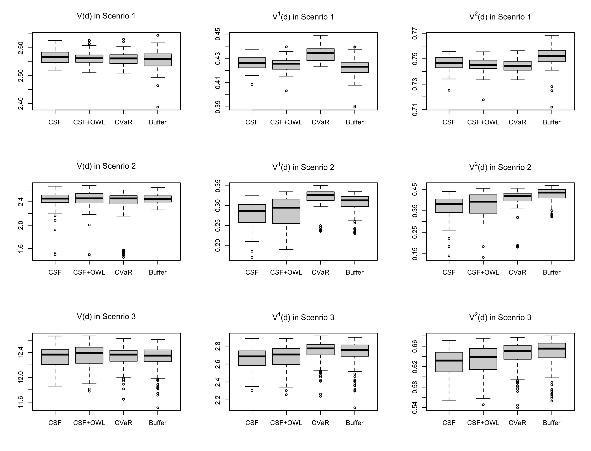
Figure 2: Boxplot of empirical value functions ($n=500$)

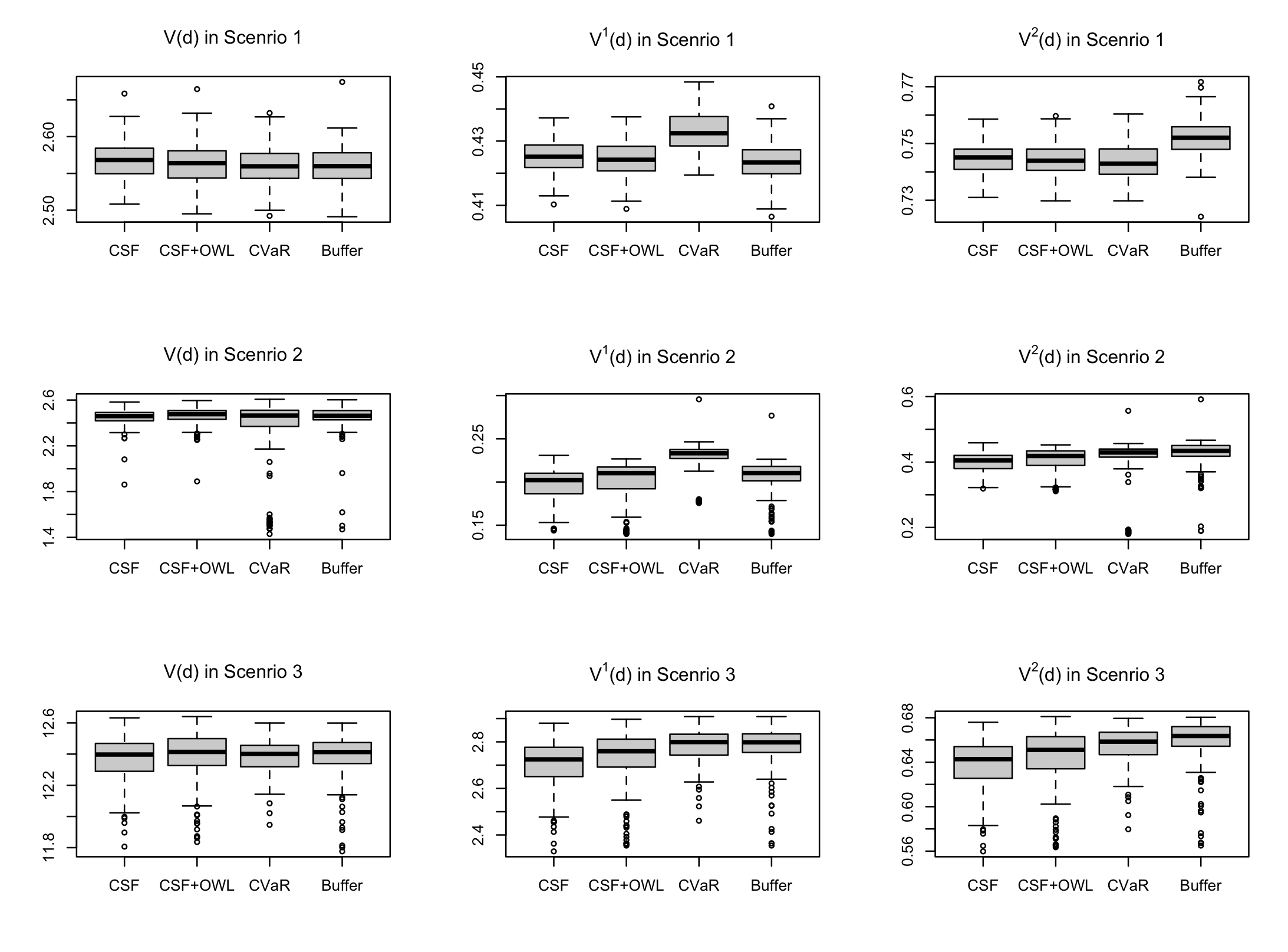
Figure 3: Boxplot of empirical value functions ($n=1000$)

6 Real data application

We consider a randomized, double-blind, placebo-controlled trial AIDS Clinical Trials Group Protocol 175 (ACTG175) (Hammer et al., 1996) with survival time as a primary outcome. The original study designs four treatment groups with patients randomly allocated: one group receives 200 mg of zidovudine three times daily, one group is provided with 200 mg of zidovudine three times each day plus 0.75 mg of zalcitabine, one group is given 200 mg of zidovudine three times daily plus 200 mg of didanosine twice a day, while the left group is assigned 200 mg of didanosine twice daily.

Following Cui et al. (2023), we focus on 1083 patients receiving treatment ZDV+ddI (561 subjects) and ddI monotherapy (522 subjects). The censoring percentage is around 21%. The selected seven discrete baseline covariates include gender (904 male and 179 female), homosexual activity (725 yes and 358 no), race (772 white and 311 non-white), symptomatic status (192 symptomatic and 891 asymptomatic), history of intravenous drug use (142 yes and 941 no), hemophilia (92 yes and 991 no), and antiretroviral history (632 experienced and 451 naive). The selected five continuous baseline covariates are age, weight, Karnofsky score (scale of 0-100), CD4 count and CD8 count.

We divide all observations into five equal proportions and use four parts as training data and the other part as testing data to apply cross-validation. The cross-validated values are obtained by averaging the empirical values on all testing subsets. We then repeat the above process for $200$ times to evaluate the performance of various methods. We consider the following performance measures:

$$\tilde{V}(d) =\mathbb{P}\left\{\mathbb{P}_{n_{test}}\left[\frac{I\{A=d(X)\}}{\pi(A|X)}\frac{\Delta Y}{\hat{S}_{C}(Y|X,A)}\right]\right\},$$

$$\tilde{V}^{1}(d) =\mathbb{P}\left\{\mathbb{P}_{n_{test}}\left[\frac{I\{A=d(X)\}}{\pi(A|X)}\left(\hat{\alpha}\gamma-\frac{\Delta(\hat{\alpha}-Y)I(\alpha>Y)}{\hat{S}_{C}(Y|X,A)}\right)\right]\right\},$$

$$\tilde{M}^{2}(d) =\mathbb{P}\left\{\mathbb{P}_{n_{test}}\left[\frac{I\{A=d(X)\}}{\pi(A|X)}\frac{\Delta\max(0,\hat{c}(-Y+\tau)+1)}{\hat{S}_{C}(Y|X,A)}\right]\right\},$$

where the outer empirical mean refers to the average over cross-validated sets, $\pi(1|X)$ is taken as 1/2, and $\hat{\alpha}$ and $\hat{c}$ are estimated from CVaR and buffered criteria.

We present values $\tilde{V}(d),\tilde{V}^{1}(d),\tilde{M}^{2}(d)$ for four methods in Table 1 with $\gamma=0.50,\tau=800.00$. In addition to a similar performance in optimizing $\tilde{V}(d)$, as expected, the proposed framework works well in tail control. For $\tilde{V}^{1}(d)$, the proposed CVaR method dominates the other three methods. Meanwhile, the Buffer method has superior performance among all other methods in minimizing $\tilde{M}^{2}(d)$.

Table 1: Numerical results for HIV data (standard deviation in brackets). Larger values of $\tilde{V}(d)$ and $\tilde{V}^{1}(d)$ are more desirable, while smaller values of $\tilde{M}^{2}(d)$ are preferred.

Method	$\tilde{V}(d)$	$\tilde{V}^{1}(d)$	$\tilde{M}^{2}(d)$
CSF	964.47  (19.63)	441.62  (34.01)	0.84  (1.00)
CSF + OWL	962.72  (19.55)	434.04  (32.88)	0.87   (1.06)
CVaR	963.29  (19.68)	448.33  (33.24)	0.86  (1.03)
Buffer	966.47  (17.80)	437.56  (33.85)	0.79  (0.92)

7 Discussion

In this paper, we propose a novel framework to estimate the optimal treatment rules in order to control the lower tail of the subjects’ survival time with right-censored data. The proposed methods directly target at quantile restricted mean survival time and survival probabilities, which are of great interest in survival analysis. For the first criterion, we maximize the restricted mean survival time, by choosing a user-specified quantile endpoint; for the second criterion, we maximize survivor function at a quality adjusted survival time, where the quality adjusted survival time is defined by restricted mean survival time. Moreover, the proposed methods have intrinsic connections to CVaR and bPOE, thus the resulting optimal rules can potentially prevent adverse events.

The proposed method can be extended in several directions. In particular, trials with multiple treatment arms occur frequently. Thus, a potential extension of our method is in the direction of angle-based methods and multicategory classification (Qiao and Liu, 2009; Sun et al., 2017; Zhou et al., 2018; Qi et al., 2019b; Zhou et al., 2022). In addition, personalized dose finding (Chen et al., 2016; Zhou et al., 2021) with a tail control might be also of interest. Furthermore, the proposed methods can be extended to mobile health dynamic treatment rules where a sequence of decision rules needs to be learned (Murphy, 2003; Robins, 2004; Zhang et al., 2013; Laber et al., 2014; Zhao et al., 2015a; Luckett et al., 2019). Finally, it would be interesting to consider an augmented inverse probability weighted estimator (Robins et al., 1994) to construct doubly robust treatment rules (Zhang et al., 2012b; Zhao et al., 2015b; Liu et al., 2018) for our proposed value functions.

Appendix

Appendix A Proofs of Equations (1) and (2)

For (1), note that

$$\bar{d} =\arg\max_{d}V(d)$$

$$=\arg\max_{d}\mathbb{E}^{d}[T]$$

$$=\arg\max_{d}\mathbb{E}[T(1)d\left(X\right)+T(0)\left(1-d\left(X\right)\right)]$$

$$=\arg\max_{d}\mathbb{E}\left[\frac{TI\{A=d(X)\}}{\pi(A|X)}\right].$$

For (2), the proof follows from the fact that the sum of the objective functions in the right hand side of (1) and (2) is a constant, i.e.,

$$\bar{d} =\arg\max_{d}\mathbb{E}\left[\frac{TI\{A=d(X)\}}{\pi(A|X)}\right]$$

$$=\arg\min_{d}\mathbb{E}\left[\frac{T}{\pi(A|X)}\right]-\mathbb{E}\left[\frac{TI\{A=d(X)\}}{\pi(A|X)}\right]$$

$$=\arg\min_{d}\mathbb{E}\left[\frac{T(1-I\{A=d(X)\})}{\pi(A|X)}\right]$$

$$=\arg\min_{d}\mathbb{E}\left[\frac{TI\{A\neq d(X)\}}{\pi(A|X)}\right].$$

Appendix B Proof of asymptotic properties for the first estimated rule

To simplify notation, we omit the supindex 1 for $V$ throughout the section.

Proof of Theorem 3.1.

Note that ${\mathcal{L}}(u)+{\mathcal{L}}(-u)=2$ for any $u$. For any $\alpha$ and measurable function $f$, we have

$$V^{\prime}_{\mathcal{L}}(f,\alpha)= \mathbb{E}_{X}\Bigg{\{}{\mathcal{L}}(f(X))\mathbb{E}\left[\alpha\gamma-\frac{\Delta(\alpha-Y)I(\alpha\geq Y)}{\widetilde{S}_{C}(Y|X,A)}|X,A=1\right]$$

$$+{\mathcal{L}}(-f(X))\mathbb{E}\left[\alpha\gamma-\frac{\Delta(\alpha-Y)I(\alpha\geq Y)}{\widetilde{S}_{C}(Y|X,A)}|X,A=-1\right]\Bigg{\}}$$

$$= \mathbb{E}_{X}\Bigg{\{}{\mathcal{L}}(f(X))\Bigg{(}\mathbb{E}\left[\alpha\gamma-\frac{\Delta(\alpha-Y)I(\alpha\geq Y)}{\widetilde{S}_{C}(Y|X,A)}|X,A=1\right]$$

$$-\mathbb{E}\left[\alpha\gamma-\frac{\Delta(\alpha-Y)I(\alpha\geq Y)}{\widetilde{S}_{C}(Y|X,A)}|X,A=-1\right]\Bigg{)}\Bigg{\}}$$

$$+2\mathbb{E}_{X}\mathbb{E}\left[\alpha\gamma-\frac{\Delta(\alpha-Y)I(\alpha\geq Y)}{\widetilde{S}_{C}(Y|X,A)}|X,A=-1\right].$$

Define

$$\beta(X)\equiv \beta_{1}(X)-\beta_{-1}(X)$$

$$\equiv \mathbb{E}[\alpha\gamma-\frac{\Delta(\alpha-Y)I(\alpha\geq Y)}{\widetilde{S}_{C}(Y|X,A)}|X,A=1]-\mathbb{E}[\alpha\gamma-\frac{\Delta(\alpha-Y)I(\alpha\geq Y)}{\widetilde{S}_{C}(Y|X,A)}|X,A=-1].$$

Without loss of generality, we assume $\beta(X)\neq 0$. If $\beta(X)>0$ for a given $\alpha$, in order to maximize $V^{\prime}_{\mathcal{L}}(f,\alpha)$, we need ${\mathcal{L}}(f(X))=2$, i.e., $f(X)\geq\delta$; similarly, if $\beta(X)<0$, we need ${\mathcal{L}}(f(X))=0$, i.e., $f(X)\leq-\delta$. Therefore, we have $|\widetilde{f}(X)|\geq\delta$ for any $X\in{\mathcal{X}}$ and

$$\max_{\begin{subarray}{c}\alpha\in\mathbb{R},||f||_{\infty}\geq\delta\end{subarray}}V^{\prime}_{\mathcal{L}}(f,\alpha)=\max_{f,\,\alpha\in\mathbb{R}}V^{\prime}_{\mathcal{L}}(f,\alpha).$$ (15)

Furthermore, it is easy to see that

$$\max_{\begin{subarray}{c}\alpha\in\mathbb{R},||f||_{\infty}\geq\delta\end{subarray}}V^{\prime}_{\mathcal{L}}(f,\alpha)=2\max_{\begin{subarray}{c}\alpha\in\mathbb{R}\end{subarray}}\mathbb{E}_{X}[{I}(\beta(X)>0)\beta_{1}(X)+{I}(\beta(X)<0)\beta_{-1}(X)].$$ (16)

Recall that $\widetilde{\alpha}$ maximizes the right hand side of Equation (16) and consequently ${\text{sign}}(\widetilde{f})={\text{sign}}(\beta^{\star})$, where $\beta^{\star}$ is defined as

$$\beta^{\star}(X)\equiv \beta_{1}^{\star}(X)-\beta_{-1}^{\star}(X)$$

$$\equiv \mathbb{E}[\widetilde{\alpha}\gamma-\frac{\Delta(\widetilde{\alpha}-Y)I(\widetilde{\alpha}\geq Y)}{\widetilde{S}_{C}(Y|X,A)}|X,A=1]-\mathbb{E}[\widetilde{\alpha}\gamma-\frac{\Delta(\widetilde{\alpha}-Y)I(\widetilde{\alpha}\geq Y)}{\widetilde{S}_{C}(Y|X,A)}|X,A=-1].$$

We can also express $V^{\prime}(d,\alpha)$ as

$$V^{\prime}(d,\alpha)= \mathbb{E}_{X}\Bigg{\{}{I}(d(X)=1)\Bigg{(}\mathbb{E}\left[\alpha\gamma-\frac{\Delta(\alpha-Y)I(\alpha\geq Y)}{\widetilde{S}_{C}(Y|X,A)}|X,A=1\right]$$

$$-\mathbb{E}\left[\alpha\gamma-\frac{\Delta(\alpha-Y)I(\alpha\geq Y)}{\widetilde{S}_{C}(Y|X,A)}|X,A=-1\right]\Bigg{)}\Bigg{\}}$$

$$+\mathbb{E}_{X}\mathbb{E}\left[\alpha\gamma-\frac{\Delta(\alpha-Y)I(\alpha\geq Y)}{\widetilde{S}_{C}(Y|X,A)}|X,A=-1\right]$$

$$= \mathbb{E}_{X}[{I}(d(X)=1)\beta(X)+\beta_{-1}(X)].$$

Thus, in order to maximize $V^{\prime}(d,\alpha)$, we have $d={\text{sign}}(\beta)$ and

$$\max_{d,\alpha\in\mathbb{R}}V^{\prime}(d,\alpha)=\max_{\alpha\in\mathbb{R}}\,\mathbb{E}_{X}[{I}(\beta(X)>0)\beta_{1}(X)+{I}(\beta(X)<0)\beta_{-1}(X)].$$ (17)

Combining Equations (15)-(17), we have that $({\text{sign}}(\widetilde{f}),\widetilde{\alpha})$ maximizes $V^{\prime}(d,\alpha)$. ∎

Proof of Theorem 3.2.

Denote $(d_{0},\alpha_{0})$ as the maximizer of $V^{\prime}({\text{sign}}(f),\alpha)$. For any measurable function $f$ and $\alpha$, we have

$$\mathbb{E}[\frac{{\mathcal{L}}(A\widetilde{f}(X))}{\pi(A|X)}(\widetilde{\alpha}\gamma-\frac{\Delta(\widetilde{\alpha}-Y)I(\widetilde{\alpha}\geq Y)}{\widetilde{S}_{C}(Y|X,A)})|X]-\mathbb{E}[\frac{{\mathcal{L}}(Af(X))}{\pi(A|X)}(\alpha\gamma-\frac{\Delta(\alpha-Y)I(\alpha\geq Y)}{\widetilde{S}_{C}(Y|X,A)})|X]$$

$$= {\mathcal{L}}(\widetilde{f}(X))\beta^{\star}_{1}+{\mathcal{L}}(-\widetilde{f}(X))\beta^{\star}_{-1}-({\mathcal{L}}(f(X))\beta_{1}+{\mathcal{L}}(-f(X))\beta_{-1}).$$

Similarly, by Theorem 3.1,

$$\mathbb{E}[\frac{I(d_{0}(X)=A)}{\pi(A|X)}(\alpha_{0}\gamma-\frac{\Delta(\alpha_{0}-Y)I(\alpha_{0}\geq Y)}{\widetilde{S}_{C}(Y|X,A)})|X]-\mathbb{E}[\frac{I(d(X)=A)}{\pi(A|X)}(\alpha\gamma-\frac{\Delta(\alpha-Y)I(\alpha\geq Y)}{\widetilde{S}_{C}(Y|X,A)})|X]$$

$$= I(d_{0}(X)=1)\beta^{\star}_{1}+I(d_{0}(X)=-1)\beta^{\star}_{-1}-I({\text{sign}}(f(X))=1)\beta_{1}-I({\text{sign}}(f(X))=-1)\beta_{-1}.$$

When $\beta^{\star}_{1}>\beta^{\star}_{-1}$, we have $\widetilde{f}\geq\delta$ and $d_{0}(X)=1$, then we have

$${\mathcal{L}}(\widetilde{f}(X))\beta^{\star}_{1}+{\mathcal{L}}(-\widetilde{f}(X))\beta^{\star}_{-1}-{\mathcal{L}}(f(X))\beta_{1}-{\mathcal{L}}(-f(X))\beta_{-1}$$

$$= 2\beta^{\star}_{1}-{\mathcal{L}}(f(X))\beta_{1}-{\mathcal{L}}(-f(X))\beta_{-1}$$

$$= 2(\beta^{\star}_{1}-\beta_{1})+{\mathcal{L}}(-f(X))\beta,$$

and

$$I(d_{0}(X)=1)\beta^{\star}_{1}+I(d_{0}(X)=-1)\beta^{\star}_{-1}-I({\text{sign}}(f(X))=1)\beta_{1}-I({\text{sign}}(f(X))=-1)\beta_{-1}$$

$$= \beta^{\star}_{1}-I({\text{sign}}(f(X))=1)\beta_{1}-I({\text{sign}}(f(X))=-1)\beta_{-1}$$

$$= (\beta^{\star}_{1}-\beta_{1})+I({\text{sign}}(f(X))=-1)\beta.$$

Note that, for any measurable function $f$, $0\leq{\mathcal{L}}(-f(X))-I({\text{sign}}(f(X))=-1)\leq 1$. Thus, we have

$$2(\beta^{\star}_{1}-\beta_{1})+{\mathcal{L}}(-f(X))\beta-\{(\beta^{\star}_{1}-\beta_{1})+I({\text{sign}}(f(X))=-1)\beta\}$$

$$= (\beta^{\star}_{1}-\beta_{1})+({\mathcal{L}}(-f(X))-I({\text{sign}}(f(X))=-1))\beta$$

$$\geq \beta_{1}^{\star}-(\beta_{1}I(\beta>0)+\beta_{-1}I(\beta<0)).$$

When $\beta^{\star}_{1}<\beta^{\star}_{-1}$, we have $\widetilde{f}\leq-\delta$ and $d_{0}(X)=-1$, then we have

$${\mathcal{L}}(\widetilde{f}(X))\beta^{\star}_{1}+{\mathcal{L}}(-\widetilde{f}(X))\beta^{\star}_{-1}-{\mathcal{L}}(f(X))\beta_{1}-{\mathcal{L}}(-f(X))\beta_{-1}$$

$$= 2\beta^{\star}_{-1}-{\mathcal{L}}(f(X))\beta_{1}-{\mathcal{L}}(-f(X))\beta_{-1}$$

$$= 2(\beta^{\star}_{-1}-\beta_{-1})+{\mathcal{L}}(f(X))\beta,$$

and

$$I(d_{0}(X)=1)\beta^{\star}_{1}+I(d_{0}(X)=-1)\beta^{\star}_{-1}-I({\text{sign}}(f(X))=1)\beta_{1}-I({\text{sign}}(f(X))=-1)\beta_{-1}$$

$$= \beta^{\star}_{-1}-I({\text{sign}}(f(X))=1)\beta_{1}-I({\text{sign}}(f(X))=-1)\beta_{-1}$$

$$= (\beta^{\star}_{-1}-\beta_{-1})+I({\text{sign}}(f(X))=1)\beta.$$

Note that, for any measurable function $f$, $0\leq{\mathcal{L}}(f(X))-I({\text{sign}}(f(X))=1)\leq 1$. Thus, we have

$$2(\beta^{\star}_{-1}-\beta_{-1})+{\mathcal{L}}(f(X))\beta-(\beta^{\star}_{-1}-\beta_{-1})+I({\text{sign}}(f(X))=1)\beta$$

$$\geq \beta_{-1}^{\star}-(\beta_{1}I(\beta>0)+\beta_{-1}I(\beta<0)).$$

Therefore, for both cases, we have

$$V^{\prime}_{\mathcal{L}}(\widetilde{f},\widetilde{\alpha})-V^{\prime}_{\mathcal{L}}(f,\alpha)-V^{\prime}(d_{0},\alpha_{0})-V^{\prime}({\text{sign}}(f),\alpha)$$

$$\geq \mathbb{E}_{X}[I(\beta^{\star}>0)\{\beta_{1}^{\star}-(\beta_{1}I(\beta>0)+\beta_{-1}I(\beta<0)\}+I(\beta^{\star}<0)\{\beta_{-1}^{\star}-(\beta_{1}I(\beta>0)+\beta_{-1}I(\beta<0))\}]$$

$$= \mathbb{E}_{X}[I(\beta^{\star}>0)\beta_{1}^{\star}+I(\beta^{\star}<0)\beta_{-1}^{\star}-(\beta_{1}I(\beta>0)+\beta_{-1}I(\beta<0)\}$$

$$\geq 0.$$

∎

Proof of Theorem 3.3.

We have the following decomposition of $V({\text{sign}}(f^{\star}),\alpha^{\star})-\sup_{\alpha\in\mathbb{R}}V({\text{sign}}(\widehat{f}),{\alpha})$,

$$V({\text{sign}}(f^{\star}),\alpha^{\star})-\sup_{\alpha\in\mathbb{R}}V({\text{sign}}(\widehat{f}),{\alpha})$$

$$\leq V({\text{sign}}(f^{\star}),\alpha^{\star})-V({\text{sign}}(\widehat{f}),\widehat{\alpha})$$

$$= V({\text{sign}}(f^{\star}),\alpha^{\star})-\sup_{f\in{\mathcal{F}},\alpha\in\mathbb{R}}V^{\prime}({\text{sign}}(f),\alpha)+\sup_{f\in{\mathcal{F}},\alpha\in\mathbb{R}}V^{\prime}({\text{sign}}(f),\alpha)$$

$$-V^{\prime}({\text{sign}}(\widehat{f}),\widehat{\alpha})+V^{\prime}({\text{sign}}(\widehat{f}),\widehat{\alpha})-V({\text{sign}}(\widehat{f}),\widehat{\alpha})$$

$$\leq V({\text{sign}}(f^{\star}),\alpha^{\star})-V^{\prime}({\text{sign}}(f^{\star}),\alpha^{\star})+\sup_{f\in{\mathcal{F}},\alpha\in\mathbb{R}}V^{\prime}({\text{sign}}(f),\alpha)$$

$$-V^{\prime}({\text{sign}}(\widehat{f}),\widehat{\alpha})+V^{\prime}({\text{sign}}(\widehat{f}),\widehat{\alpha})-V({\text{sign}}(\widehat{f}),\widehat{\alpha})$$

$$\leq 2\sup_{f\in{\mathcal{F}},\alpha\in\mathbb{R}}|V({\text{sign}}(f),\alpha)-V^{\prime}({\text{sign}}(f),\alpha)|+\sup_{f\in{\mathcal{F}},\alpha\in\mathbb{R}}V^{\prime}({\text{sign}}(f),\alpha)-V^{\prime}({\text{sign}}(\widehat{f}),\widehat{\alpha}).$$

For the first term,

$$\sup_{f\in{\mathcal{F}},\alpha\in\mathbb{R}}|V({\text{sign}}(f),\alpha)-V^{\prime}({\text{sign}}(f),\alpha)|$$

$$= \sup_{f\in{\mathcal{F}},\alpha\in\mathbb{R}}\mathbb{E}\Bigg{\{}\bigg{|}\frac{\Delta(\alpha-Y)I(\alpha\geq Y)}{S_{C}(Y|X,A)}-\frac{\Delta(\alpha-Y)I(\alpha\geq Y)}{\widetilde{S}_{C}(Y|X,A)}\bigg{|}\frac{I\{A={\text{sign}}(f(X))\}}{\pi(A|X)}\Bigg{\}}$$

$$= 0.$$ (18)

For the second term, by the excess risk value bound established in Theorem 3.2, we have

$$\sup_{f\in{\mathcal{F}},\alpha\in\mathbb{R}}V^{\prime}({\text{sign}}(f),\alpha)-V^{\prime}({\text{sign}}(\widehat{f}),\widehat{\alpha})\leq V^{\prime}_{\mathcal{L}}(\widetilde{f},\widetilde{\alpha})-V^{\prime}_{\mathcal{L}}(\widehat{f},\widehat{\alpha}).$$

By Theorem 4.1, we have that

$$\frac{1}{n}\sum_{i=1}^{n}\frac{{\mathcal{L}}(A_{i}\widetilde{f}(X_{i}))}{\pi(A_{i}|X_{i})}\left\{\widetilde{\alpha}\gamma-\frac{\Delta_{i}(\widetilde{\alpha}-Y_{i})I(Y_{i}\leq\widetilde{\alpha})}{\widehat{S}_{C}(Y_{i}|X_{i},A_{i})}\right\}$$

$$\leq \frac{1}{n}\sum_{i=1}^{n}\frac{{\mathcal{L}}(A_{i}\widehat{f}(X_{i}))}{\pi(A_{i}|X_{i})}\left\{\widehat{\alpha}\gamma-\frac{\Delta_{i}(\widehat{\alpha}-Y_{i})I(Y_{i}\leq\widehat{\alpha})}{\widehat{S}_{C}(Y_{i}|X_{i},A_{i})}\right\}.$$

So we have

$$V^{\prime}_{\mathcal{L}}(\widetilde{f},\widetilde{\alpha})-V^{\prime}_{\mathcal{L}}(\widehat{f},\widehat{\alpha})$$

$$\leq V^{\prime}_{\mathcal{L}}(\widetilde{f},\widetilde{\alpha})-V^{\prime}_{\mathcal{L}}(\widehat{f},\widehat{\alpha})$$

$$+ \frac{1}{n}\sum_{i=1}^{n}\frac{{\mathcal{L}}(A_{i}\widehat{f}(X_{i}))}{\pi(A_{i}|X_{i})}\left\{\widehat{\alpha}\gamma-\frac{\Delta_{i}(\widehat{\alpha}-Y_{i})I(Y_{i}\leq\widehat{\alpha})}{\widehat{S}_{C}(Y_{i}|X_{i},A_{i})}\right\}$$

$$- \frac{1}{n}\sum_{i=1}^{n}\frac{{\mathcal{L}}(A_{i}\widetilde{f}(X_{i}))}{\pi(A_{i}|X_{i})}\left\{\widetilde{\alpha}\gamma-\frac{\Delta_{i}(\widetilde{\alpha}-Y_{i})I(Y_{i}\leq\widetilde{\alpha})}{\widehat{S}_{C}(Y_{i}|X_{i},A_{i})}\right\}$$

$$+ \mathbb{E}\left[\frac{{\mathcal{L}}(A\widetilde{f}(X))}{\pi(A|X)}\left\{\widetilde{\alpha}\gamma-\frac{\Delta(\widetilde{\alpha}-Y)I(Y\leq\widetilde{\alpha})}{\widehat{S}_{C}(Y|X,A)}\right\}\right]-\mathbb{E}\left[\frac{{\mathcal{L}}(A\widetilde{f}(X))}{\pi(A|X)}\left\{\widetilde{\alpha}\gamma-\frac{\Delta(\widetilde{\alpha}-Y)I(Y\leq\widetilde{\alpha})}{\widehat{S}_{C}(Y|X,A)}\right\}\right]$$

$$+ \mathbb{E}\left[\frac{{\mathcal{L}}(A\widehat{f}(X))}{\pi(A|X)}\left\{\widehat{\alpha}\gamma-\frac{\Delta(\widehat{\alpha}-Y)I(Y\leq\widehat{\alpha})}{\widehat{S}_{C}(Y|X,A)}\right\}\right]-\mathbb{E}\left[\frac{{\mathcal{L}}(A\widehat{f}(X))}{\pi(A|X)}\left\{\widehat{\alpha}\gamma-\frac{\Delta(\widehat{\alpha}-Y)I(Y\leq\widehat{\alpha})}{\widehat{S}_{C}(Y|X,A)}\right\}\right].$$

It is easy to see that

$$|V^{\prime}_{\mathcal{L}}(\widetilde{f},\widetilde{\alpha})-V^{\wedge}_{\mathcal{L}}(\widetilde{f},\widetilde{\alpha})|\overset{p}{\to}0,$$

and

$$|V^{\prime}_{\mathcal{L}}(\widehat{f},\widehat{\alpha})-V^{\wedge}_{\mathcal{L}}(\widehat{f},\widehat{\alpha})|\overset{p}{\to}0.$$

So the remaining part is to show

$$\frac{1}{n}\sum_{i=1}^{n}\frac{{\mathcal{L}}(A_{i}\widehat{f}(X_{i}))}{\pi(A_{i}|X_{i})}\left\{\widehat{\alpha}\gamma-\frac{\Delta_{i}(\widehat{\alpha}-Y_{i})I(Y_{i}\leq\widehat{\alpha})}{\widehat{S}_{C}(Y_{i}|X_{i},A_{i})}\right\}-\left(V^{\wedge}_{\mathcal{L}}(\widehat{f},\widehat{\alpha})\right)$$

$$- \left[\frac{1}{n}\sum_{i=1}^{n}\frac{{\mathcal{L}}(A_{i}\widetilde{f}(X_{i}))}{\pi(A_{i}|X_{i})}\left\{\widetilde{\alpha}\gamma-\frac{\Delta_{i}(\widetilde{\alpha}-Y_{i})I(Y_{i}\leq\widetilde{\alpha})}{\widehat{S}_{C}(Y_{i}|X_{i},A_{i})}\right\}-\left(V^{\wedge}_{\mathcal{L}}(\widetilde{f},\widetilde{\alpha})\right)\right]\overset{p}{\to}0,$$

which follows standard empirical process theory. Combining with Equation (18) completes the proof. ∎

Appendix C Proof of asymptotic properties for the second estimated rule

To simplify notation, we omit the supindex 2 for $V$ throughout the section.

Proof of Theorem 3.4.

Note that ${\mathcal{L}}(u)+{\mathcal{L}}(-u)=2$ for any $u$. For any $c\geq 0$ and measurable function $f$, we have

$$V^{\prime}_{\mathcal{L}}(f,c)= \mathbb{E}_{X}\Bigg{\{}{\mathcal{L}}(f(X))\mathbb{E}\left[-\frac{\max(0,c(-Y+\tau)+1)}{\widetilde{S}_{C}(Y|X,A)}|X,A=1\right]$$

$$+{\mathcal{L}}(-f(X))\mathbb{E}\left[-\frac{\max(0,c(-Y+\tau)+1)}{\widetilde{S}_{C}(Y|X,A)}|X,A=-1\right]\Bigg{\}}$$

$$= \mathbb{E}_{X}\Bigg{\{}{\mathcal{L}}(f(X))\Bigg{(}\mathbb{E}\left[-\frac{\max(0,c(-Y+\tau)+1)}{\widetilde{S}_{C}(Y|X,A)}|X,A=1\right]$$

$$-\mathbb{E}\left[-\frac{\max(0,c(-Y+\tau)+1)}{\widetilde{S}_{C}(Y|X,A)}|X,A=-1\right]\Bigg{)}\Bigg{\}}$$

$$+2\mathbb{E}_{X}\mathbb{E}\left[-\frac{\max(0,c(-Y+\tau)+1)}{\widetilde{S}_{C}(Y|X,A)}|X,A=-1\right].$$

Define

$$\beta(X)\equiv \beta_{1}(X)-\beta_{-1}(X)$$

$$\equiv \mathbb{E}[-\frac{\max(0,c(-Y+\tau)+1)}{\widetilde{S}_{C}(Y|X,A)}|X,A=1]-\mathbb{E}[-\frac{\max(0,c(-Y+\tau)+1)}{\widetilde{S}_{C}(Y|X,A)}|X,A=-1].$$

Without loss of generality, we assume $\beta(X)\neq 0$. If $\beta(X)>0$ for a given $c$, in order to maximize $V^{\prime}_{\mathcal{L}}(f,c)$, we need ${\mathcal{L}}(f(X))=2$, i.e., $f(X)\geq\delta$; similarly, if $\beta(X)<0$, we need ${\mathcal{L}}(f(X))=0$, i.e., $f(X)\leq-\delta$. Therefore, we have $|\widetilde{f}(X)|\geq\delta$ for any $X\in{\mathcal{X}}$ and

$$\max_{\begin{subarray}{c}c\geq 0,||f||_{\infty}\geq\delta\end{subarray}}V^{\prime}_{\mathcal{L}}(f,c)=\max_{f,\,c\geq 0}V^{\prime}_{\mathcal{L}}(f,c).$$ (19)

Furthermore, it is easy to see that

$$\max_{\begin{subarray}{c}c\geq 0,||f||_{\infty}\geq\delta\end{subarray}}V^{\prime}_{\mathcal{L}}(f,c)=2\max_{\begin{subarray}{c}c\geq 0\end{subarray}}\mathbb{E}_{X}[{I}(\beta(X)>0)\beta_{1}(X)+{I}(\beta(X)<0)\beta_{-1}(X)].$$ (20)

Recall that $\widetilde{c}$ maximizes the right hand side of Equation (20) and consequently ${\text{sign}}(\widetilde{f})={\text{sign}}(\beta^{\star})$, where $\beta^{\star}$ is defined as

$$\beta^{\star}(X)\equiv \beta_{1}^{\star}(X)-\beta_{-1}^{\star}(X)$$

$$\equiv \mathbb{E}[-\frac{\max(0,\widetilde{c}(-Y+\tau)+1)}{\widetilde{S}_{C}(Y|X,A)}|X,A=1]-\mathbb{E}[-\frac{\max(0,\widetilde{c}(-Y+\tau)+1)}{\widetilde{S}_{C}(Y|X,A)}|X,A=-1].$$

We can also express $V^{\prime}(d,c)$ as

$$V^{\prime}(d,c)= \mathbb{E}_{X}\Bigg{\{}{I}(d(X)=1)\Bigg{(}\mathbb{E}\left[-\frac{\max(0,\widetilde{c}(-Y+\tau)+1)}{\widetilde{S}_{C}(Y|X,A)}|X,A=1\right]$$

$$-\mathbb{E}\left[-\frac{\max(0,\widetilde{c}(-Y+\tau)+1)}{\widetilde{S}_{C}(Y|X,A)}|X,A=-1\right]\Bigg{)}\Bigg{\}}$$

$$+\mathbb{E}_{X}\mathbb{E}\left[-\frac{\max(0,\widetilde{c}(-Y+\tau)+1)}{\widetilde{S}_{C}(Y|X,A)}|X,A=-1\right]$$

$$= \mathbb{E}_{X}[{I}(d(X)=1)\beta(X)+\beta_{-1}(X)].$$

Thus, in order to maximize $V^{\prime}(d,c)$, we have $d={\text{sign}}(\beta)$ and

$$\max_{d,c\geq 0}V^{\prime}(d,c)=\max_{c\geq 0}\,\mathbb{E}_{X}[{I}(\beta(X)>0)\beta_{1}(X)+{I}(\beta(X)<0)\beta_{-1}(X)].$$ (21)

Combining Equations (19)-(21), we have that $({\text{sign}}(\widetilde{f}),\widetilde{c})$ maximizes $V^{\prime}(d,c)$. ∎

Proof of Theorem 3.5.

Denote $(d_{0},c_{0})$ as the maximizer of $V^{\prime}({\text{sign}}(f),c)$. For any measurable function $f$ and $c\geq 0$, we have

$$\mathbb{E}[\frac{{\mathcal{L}}(A\widetilde{f}(X))}{\pi(A|X)}(-\frac{\max(0,\widetilde{c}(-Y+\tau)+1)}{\widetilde{S}_{C}(Y|X,A)})|X]-\mathbb{E}[\frac{{\mathcal{L}}(Af(X))}{\pi(A|X)}(-\frac{\max(0,c(-Y+\tau)+1)}{\widetilde{S}_{C}(Y|X,A)})|X]$$

$$= {\mathcal{L}}(\widetilde{f}(X))\beta^{\star}_{1}+{\mathcal{L}}(-\widetilde{f}(X))\beta^{\star}_{-1}-({\mathcal{L}}(f(X))\beta_{1}+{\mathcal{L}}(-f(X))\beta_{-1}).$$

Similarly, by Theorem 3.4,

$$\mathbb{E}[\frac{I(d_{0}(X)=A)}{\pi(A|X)}(-\frac{\max(0,c_{0}(-Y+\tau)+1)}{\widetilde{S}_{C}(Y|X,A)})|X]-\mathbb{E}[\frac{I(d(X)=A)}{\pi(A|X)}(-\frac{\max(0,c(-Y+\tau)+1)}{\widetilde{S}_{C}(Y|X,A)})|X]$$

$$= I(d_{0}(X)=1)\beta^{\star}_{1}+I(d_{0}(X)=-1)\beta^{\star}_{-1}-I({\text{sign}}(f(X))=1)\beta_{1}-I({\text{sign}}(f(X))=-1)\beta_{-1}.$$

When $\beta^{\star}_{1}>\beta^{\star}_{-1}$, we have $\widetilde{f}\geq\delta$ and $d_{0}(X)=1$, then we have

$${\mathcal{L}}(\widetilde{f}(X))\beta^{\star}_{1}+{\mathcal{L}}(-\widetilde{f}(X))\beta^{\star}_{-1}-{\mathcal{L}}(f(X))\beta_{1}-{\mathcal{L}}(-f(X))\beta_{-1}$$

$$= 2\beta^{\star}_{1}-{\mathcal{L}}(f(X))\beta_{1}-{\mathcal{L}}(-f(X))\beta_{-1}$$

$$= 2(\beta^{\star}_{1}-\beta_{1})+{\mathcal{L}}(-f(X))\beta,$$

and

$$I(d_{0}(X)=1)\beta^{\star}_{1}+I(d_{0}(X)=-1)\beta^{\star}_{-1}-I({\text{sign}}(f(X))=1)\beta_{1}-I({\text{sign}}(f(X))=-1)\beta_{-1}$$

$$= \beta^{\star}_{1}-I({\text{sign}}(f(X))=1)\beta_{1}-I({\text{sign}}(f(X))=-1)\beta_{-1}$$

$$= (\beta^{\star}_{1}-\beta_{1})+I({\text{sign}}(f(X))=-1)\beta.$$

Note that, for any measurable function $f$, $0\leq{\mathcal{L}}(-f(X))-I({\text{sign}}(f(X))=-1)\leq 1$. Thus, we have

$$2(\beta^{\star}_{1}-\beta_{1})+{\mathcal{L}}(-f(X))\beta-\{(\beta^{\star}_{1}-\beta_{1})+I({\text{sign}}(f(X))=-1)\beta\}$$

$$= (\beta^{\star}_{1}-\beta_{1})+({\mathcal{L}}(-f(X))-I({\text{sign}}(f(X))=-1))\beta$$

$$\geq \beta_{1}^{\star}-(\beta_{1}I(\beta>0)+\beta_{-1}I(\beta<0)).$$

When $\beta^{\star}_{1}<\beta^{\star}_{-1}$, we have $\widetilde{f}\leq-\delta$ and $d_{0}(X)=-1$, then we have

$${\mathcal{L}}(\widetilde{f}(X))\beta^{\star}_{1}+{\mathcal{L}}(-\widetilde{f}(X))\beta^{\star}_{-1}-{\mathcal{L}}(f(X))\beta_{1}-{\mathcal{L}}(-f(X))\beta_{-1}$$

$$= 2\beta^{\star}_{-1}-{\mathcal{L}}(f(X))\beta_{1}-{\mathcal{L}}(-f(X))\beta_{-1}$$

$$= 2(\beta^{\star}_{-1}-\beta_{-1})+{\mathcal{L}}(f(X))\beta,$$

and

$$I(d_{0}(X)=1)\beta^{\star}_{1}+I(d_{0}(X)=-1)\beta^{\star}_{-1}-I({\text{sign}}(f(X))=1)\beta_{1}-I({\text{sign}}(f(X))=-1)\beta_{-1}$$

$$= \beta^{\star}_{-1}-I({\text{sign}}(f(X))=1)\beta_{1}-I({\text{sign}}(f(X))=-1)\beta_{-1}$$

$$= (\beta^{\star}_{-1}-\beta_{-1})+I({\text{sign}}(f(X))=1)\beta.$$

Note that, for any measurable function $f$, $0\leq{\mathcal{L}}(f(X))-I({\text{sign}}(f(X))=1)\leq 1$. Thus, we have

$$2(\beta^{\star}_{-1}-\beta_{-1})+{\mathcal{L}}(f(X))\beta-(\beta^{\star}_{-1}-\beta_{-1})+I({\text{sign}}(f(X))=1)\beta$$

$$\geq \beta_{-1}^{\star}-(\beta_{1}I(\beta>0)+\beta_{-1}I(\beta<0)).$$

Therefore, for both cases, we have

$$V^{\prime}_{\mathcal{L}}(\widetilde{f},\widetilde{c})-V^{\prime}_{\mathcal{L}}(f,c)-V^{\prime}(d_{0},c_{0})-V^{\prime}({\text{sign}}(f),c)$$

$$\geq \mathbb{E}_{X}[I(\beta^{\star}>0)\{\beta_{1}^{\star}-(\beta_{1}I(\beta>0)+\beta_{-1}I(\beta<0)\}+I(\beta^{\star}<0)\{\beta_{-1}^{\star}-(\beta_{1}I(\beta>0)+\beta_{-1}I(\beta<0))\}]$$

$$= \mathbb{E}_{X}[I(\beta^{\star}>0)\beta_{1}^{\star}+I(\beta^{\star}<0)\beta_{-1}^{\star}-(\beta_{1}I(\beta>0)+\beta_{-1}I(\beta<0)\}$$

$$\geq 0.$$

∎

Proof of Theorem 3.6.

We have the following decomposition of $V({\text{sign}}(f^{\star}),c^{\star})-\sup_{c\geq 0}V({\text{sign}}(\widehat{f}),{c})$,

$$V({\text{sign}}(f^{\star}),c^{\star})-\sup_{c\geq 0}V({\text{sign}}(\widehat{f}),{c})$$

$$\leq V({\text{sign}}(f^{\star}),c^{\star})-V({\text{sign}}(\widehat{f}),\widehat{c})$$

$$= V({\text{sign}}(f^{\star}),c^{\star})-\sup_{f\in{\mathcal{F}},c\geq 0}V^{\prime}({\text{sign}}(f),c)+\sup_{f\in{\mathcal{F}},c\geq 0}V^{\prime}({\text{sign}}(f),c)$$

$$-V^{\prime}({\text{sign}}(\widehat{f}),\widehat{c})+V^{\prime}({\text{sign}}(\widehat{f}),\widehat{c})-V({\text{sign}}(\widehat{f}),\widehat{c})$$

$$\leq V({\text{sign}}(f^{\star}),c^{\star})-V^{\prime}({\text{sign}}(f^{\star}),c^{\star})+\sup_{f\in{\mathcal{F}},c\geq 0}V^{\prime}({\text{sign}}(f),c)$$

$$-V^{\prime}({\text{sign}}(\widehat{f}),\widehat{c})+V^{\prime}({\text{sign}}(\widehat{f}),\widehat{c})-V({\text{sign}}(\widehat{f}),\widehat{c})$$

$$\leq 2\sup_{f\in{\mathcal{F}},c\geq 0}|V({\text{sign}}(f),c)-V^{\prime}({\text{sign}}(f),c)|+\sup_{f\in{\mathcal{F}},c\geq 0}V^{\prime}({\text{sign}}(f),c)-V^{\prime}({\text{sign}}(\widehat{f}),\widehat{c}).$$

For the first term,

$$\sup_{f\in{\mathcal{F}},c\geq 0}|V({\text{sign}}(f),c)-V^{\prime}({\text{sign}}(f),c)|$$

$$= \sup_{f\in{\mathcal{F}},c\geq 0}\mathbb{E}\Bigg{\{}\bigg{|}\frac{\Delta\max(0,c(-Y+\tau)+1)}{S_{C}(Y|X,A)}-\frac{\Delta\max(0,c(-Y+\tau)+1)}{\widetilde{S}_{C}(Y|X,A)}\bigg{|}\frac{I\{A={\text{sign}}(f(X))\}}{\pi(A|X)}\Bigg{\}}$$

$$= 0.$$ (22)

For the second term, by the excess risk value bound established in Theorem 3.5, we have

$$\sup_{f\in{\mathcal{F}},c\geq 0}V^{\prime}({\text{sign}}(f),c)-V^{\prime}({\text{sign}}(\widehat{f}),\widehat{c})\leq V^{\prime}_{\mathcal{L}}(\widetilde{f},\widetilde{c})-V^{\prime}_{\mathcal{L}}(\widehat{f},\widehat{c}).$$

By Theorem 4.1, we have that

$$\frac{1}{n}\sum_{i=1}^{n}\frac{{\mathcal{L}}(A_{i}\widetilde{f}(X_{i}))}{\pi(A_{i}|X_{i})}\left\{-\frac{\Delta_{i}\max(0,\widetilde{c}(-Y_{i}+\tau)+1)}{\widehat{S}_{C}(Y_{i}|X_{i},A_{i})}\right\}$$

$$\leq \frac{1}{n}\sum_{i=1}^{n}\frac{{\mathcal{L}}(A_{i}\widehat{f}(X_{i}))}{\pi(A_{i}|X_{i})}\left\{-\frac{\Delta_{i}\max(0,\widehat{c}(-Y_{i}+\tau)+1)}{\widehat{S}_{C}(Y_{i}|X_{i},A_{i})}\right\}.$$

So we have

$$V^{\prime}_{\mathcal{L}}(\widetilde{f},\widetilde{c})-V^{\prime}_{\mathcal{L}}(\widehat{f},\widehat{c})$$

$$\leq V^{\prime}_{\mathcal{L}}(\widetilde{f},\widetilde{c})-V^{\prime}_{\mathcal{L}}(\widehat{f},\widehat{c})$$

$$+ \frac{1}{n}\sum_{i=1}^{n}\frac{{\mathcal{L}}(A_{i}\widehat{f}(X_{i}))}{\pi(A_{i}|X_{i})}\left\{-\frac{\Delta_{i}\max(0,\widehat{c}(-Y_{i}+\tau)+1)}{\widehat{S}_{C}(Y_{i}|X_{i},A_{i})}\right\}$$

$$- \frac{1}{n}\sum_{i=1}^{n}\frac{{\mathcal{L}}(A_{i}\widetilde{f}(X_{i}))}{\pi(A_{i}|X_{i})}\left\{-\frac{\Delta_{i}\max(0,\widetilde{c}(-Y_{i}+\tau)+1)}{\widehat{S}_{C}(Y_{i}|X_{i},A_{i})}\right\}$$

$$+ \mathbb{E}\left[\frac{{\mathcal{L}}(A\widetilde{f}(X))}{\pi(A|X)}\left\{-\frac{\Delta\max(0,\widetilde{c}(-Y+\tau)+1)}{\widehat{S}_{C}(Y|X,A)}\right\}\right]-\mathbb{E}\left[\frac{{\mathcal{L}}(A\widetilde{f}(X))}{\pi(A|X)}\left\{-\frac{\Delta\max(0,\widetilde{c}(-Y+\tau)+1)}{\widehat{S}_{C}(Y|X,A)}\right\}\right]$$

$$+ \mathbb{E}\left[\frac{{\mathcal{L}}(A\widehat{f}(X))}{\pi(A|X)}\left\{-\frac{\Delta\max(0,\widehat{c}(-Y+\tau)+1)}{\widehat{S}_{C}(Y|X,A)}\right\}\right]-\mathbb{E}\left[\frac{{\mathcal{L}}(A\widehat{f}(X))}{\pi(A|X)}\left\{-\frac{\Delta\max(0,\widehat{c}(-Y+\tau)+1)}{\widehat{S}_{C}(Y|X,A)}\right\}\right].$$

It is easy to see that

$$|V^{\prime}_{\mathcal{L}}(\widetilde{f},\widetilde{c})-V^{\wedge}_{\mathcal{L}}(\widetilde{f},\widetilde{c})|\overset{p}{\to}0,$$

and

$$|V^{\prime}_{\mathcal{L}}(\widehat{f},\widehat{c})-V^{\wedge}_{\mathcal{L}}(\widehat{f},\widehat{c})|\overset{p}{\to}0.$$

So the remaining part is to show

$$\frac{1}{n}\sum_{i=1}^{n}\frac{{\mathcal{L}}(A_{i}\widehat{f}(X_{i}))}{\pi(A_{i}|X_{i})}\left\{-\frac{\Delta_{i}\max(0,\widehat{c}(-Y_{i}+\tau)+1)}{\widehat{S}_{C}(Y_{i}|X_{i},A_{i})}\right\}-\left(V^{\wedge}_{\mathcal{L}}(\widehat{f},\widehat{c})\right)$$

$$- \left[\frac{1}{n}\sum_{i=1}^{n}\frac{{\mathcal{L}}(A_{i}\widetilde{f}(X_{i}))}{\pi(A_{i}|X_{i})}\left\{-\frac{\Delta_{i}\max(0,\widetilde{c}(-Y_{i}+\tau)+1)}{\widehat{S}_{C}(Y_{i}|X_{i},A_{i})}\right\}-\left(V^{\wedge}_{\mathcal{L}}(\widetilde{f},\widetilde{c})\right)\right]\overset{p}{\to}0,$$

which follows standard empirical process theory (Kosorok, 2008). Combining with Equation (22) completes the proof. ∎

Appendix D Proof of Theorem 4.1

Lemma D.1.

For a sequence of points $\{\beta^{(\nu)}\}$ in $\mathbb{R}^{n}$ with $\lim_{\nu\to\infty}\beta^{(\nu)}=\beta^{\,\infty}$, for any $\varepsilon>0$ that is sufficiently small, there exists $\bar{\nu}$, such that $\mathcal{M}(\beta^{\,\infty})\subseteq\widetilde{\mathcal{M}}^{(\nu)}_{\varepsilon}(\beta)$ for any $\nu\geq\bar{\nu}$ with probability 1.

Proof of Lemma D.1.

From Theorem 7.53 in Shapiro et al. (2009), we can obtain that with i.i.d. generated samples $\{Z_{i}:i\in I_{\nu}\}$ of size $N_{\nu}$ from the whole data set $\{Z_{i}\}_{i=1}^{n}$, for every $j\in[n]$, $\frac{1}{N_{\nu}}\sum_{i=1}^{N_{\nu}}\,\psi(\beta,Y_{j};Z_{i})$ converges to $\frac{1}{n}\sum_{i=1}^{n}\,\psi(\beta,Y_{j};Z_{i})$ with probability 1 uniformly on a compact set in $\mathbb{R}^{d}$. Then from Proposition 5.2 in Shapiro et al. (2009), we have that for every $j\in[n]$, $\lim_{\nu\to\infty}\,\frac{1}{N_{\nu}}\sum_{i=1}^{N_{\nu}}\,\psi(\beta^{(\nu)},Y_{j};Z_{i})=\frac{1}{n}\sum_{i=1}^{n}\,\psi(\beta^{\,\infty},Y_{j};Z_{i})$ with probability 1.

Recall that $\mathcal{M}(\beta)\equiv\underset{j\in[n]}{\mbox{argmin}}\,\,\,\ \displaystyle{\frac{1}{n}\sum_{i=1}^{n}}\psi(\beta,Y_{j};Z_{i})$, and with $\varepsilon$ sufficiently small, we must have

$$\begin{array}[]{ll}\widetilde{\mathcal{M}}^{(\nu)}_{\varepsilon}(\beta)&\equiv\left\{\ell\in\mathcal{I}_{\nu}:\displaystyle{\frac{1}{N_{\nu}}\sum_{i=1}^{N_{\nu}}}\psi(\beta,Y_{\ell};Z_{i})\leq\min_{j\in\mathcal{I}_{\nu}}\,\displaystyle{\frac{1}{N_{\nu}}\sum_{i=1}^{N_{\nu}}}\psi(\beta,Y_{j};Z_{i})+\varepsilon\right\}\\[14.45377pt] &=\left\{\ell\in[n]:\displaystyle{\frac{1}{N_{\nu}}\sum_{i=1}^{N_{\nu}}}\psi(\beta,Y_{\ell};Z_{i})\leq\min_{j\in[n]}\,\displaystyle{\frac{1}{N_{\nu}}\sum_{i=1}^{N_{\nu}}}\psi(\beta,Y_{j};Z_{i})+\varepsilon\right\},\end{array}$$

where the last equation is derived since the a convex piecewise affine function achieves its minimum at one of the knots and the $\varepsilon$-active indexes must also be contained in $\mathcal{I}_{n}$ given that $\varepsilon$ is sufficiently small. Then there exists $\bar{\nu}$ such that for any $j\in\mathcal{M}(f)$, with $\nu\geq\bar{\nu}$, the following holds with probability 1,

$$\begin{array}[]{ll}\displaystyle{\frac{1}{N_{\nu}}\sum_{i=1}^{N_{\nu}}}\psi(\beta^{(\nu)},Y_{j};Z_{i})&\leq\varepsilon/2+\displaystyle{\frac{1}{n}\sum_{i=1}^{n}}\psi(\beta^{\,\infty},Y_{j};Z_{i})\\[14.45377pt] &=\varepsilon/2+\min_{j\in[n]}\displaystyle{\frac{1}{n}\sum_{i=1}^{n}}\psi(\beta^{\,\infty},Y_{j};Z_{i})\\[14.45377pt] &\leq\varepsilon+\min_{j\in[n]}\displaystyle{\frac{1}{N_{\nu}}\sum_{i=1}^{N_{\nu}}}\psi(\beta^{(\nu)},Y_{j};Z_{i})\end{array}$$

This implies that $\mathcal{M}(\beta^{\,\infty})\subseteq\widetilde{\mathcal{M}}^{(\nu)}_{\varepsilon}(\beta)$ for any $\nu\geq\bar{\nu}$ with probability 1. ∎

Proof of Theorem 4.1.

With $\widetilde{\mathcal{M}}^{(\nu)}(\beta)\equiv\underset{j\in\mathcal{I}_{\nu}}{\mbox{argmin}}\,\,\,\displaystyle{\frac{1}{N_{\nu}}\sum_{i=1}^{N_{\nu}}}\psi(\beta,Y_{j};Z_{i})$, by the update rule of the algorithm at the $\nu$th iteration, we derive

$$\begin{array}[]{lll}&&\widetilde{V}^{(\nu)}(\beta^{(\nu+1)})+\displaystyle{\frac{1}{2\rho}}\,\left\|\,\beta^{(\nu+1)}-\beta^{(\nu)}\,\right\|^{2}\\[10.84006pt] &\leq&\widetilde{V}^{(\nu)}(\beta^{(\nu+1/2)}_{j})+\displaystyle{\frac{1}{2\rho}}\,\left\|\,\beta^{(\nu+1/2)}_{j}-\beta^{(\nu)}\,\right\|^{2},\qquad\mbox{for any }j\in\widetilde{\mathcal{M}}^{(\nu)}(\beta)\\[10.84006pt] &\leq&\widehat{V}_{j}^{(\nu)}(\beta^{(\nu+1/2)}_{j};\beta^{(\nu)})+\displaystyle{\frac{1}{2\rho}}\,\left\|\,\beta_{j}^{(\nu+1/2)}-\beta^{\,(\nu)}\,\right\|^{2},\qquad\mbox{for any }j\in\widetilde{\mathcal{M}}^{(\nu)}(\beta)\\[7.22743pt] &\leq&\widehat{V}_{j}^{(\nu)}(\beta^{(\nu)};\beta^{(\nu)}),\qquad\mbox{for any }j\in\widetilde{\mathcal{M}}_{\nu}(\beta^{(\nu)})\\[7.22743pt] &=&\widetilde{V}^{(\nu)}(\beta^{\,(\nu)}).\end{array}$$ (23)

We further reformulate $\widetilde{V}^{(\nu)}(\beta^{(\nu)})$ as follows,

$$\widetilde{V}^{(\nu)}(\beta^{(\nu)})=\underset{j\in[n]}{\mbox{min}}\,\left(-\displaystyle{\frac{1}{N_{\nu-1}}}\sum_{i\in I_{\nu-1}}\,\psi(\beta^{(\nu)},Y_{j};Z_{i})+\varepsilon_{\nu,j}\right)$$

where

$$\begin{array}[]{lll}\varepsilon_{\nu,j}&\equiv&\displaystyle{\frac{1}{N_{\nu-1}}}\sum_{i\in I_{\nu-1}}\,\psi(\beta^{(\nu)},Y_{j};Z_{i})-\displaystyle{\frac{1}{N_{\nu}}}\sum_{i\in I_{\nu}}\,\psi(\beta^{(\nu)},Y_{j};Z_{i})\end{array}$$

Moreover, let $\mathcal{F}_{\nu-1}$ denote the filtration till iteration $\nu-1$, by taking the conditional expectation of $\varepsilon_{\nu,j}$, we obtain that

$$\begin{array}[]{ll}&\mathbb{E}_{\nu}\left[\,\varepsilon_{\nu,j}\mid\mathcal{F}_{\nu-1}\right]=\displaystyle{\left(\frac{1}{N_{\nu-1}}-\frac{1}{N_{\nu}}\right)}\sum_{i\in I_{\nu-1}}\,\psi(\beta^{(\nu)},Y_{j};Z_{i})-\mathbb{E}_{\nu}\bigg{[}\displaystyle{\frac{1}{N_{\nu}}}\displaystyle{\sum_{i\in K_{\nu}}}\,\psi(\beta^{\,(\nu)},Y_{j};Z_{i})\,\mid\mathcal{F}_{\nu-1}\bigg{]}\\[14.45377pt] &=\displaystyle{\frac{N_{\nu}-N_{\nu-1}}{N_{\nu}}}\,\left(\displaystyle{\frac{1}{N_{\nu-1}}}\,\displaystyle{\sum_{i\in I_{\nu-1}}}\,\psi(\beta^{\,(\nu)},Y_{j};Z_{i})-\mathbb{E}_{\nu}\bigg{[}\,\displaystyle{\frac{1}{N_{\nu}-N_{\nu-1}}}\,\displaystyle{\sum_{i\in K_{\nu}}}\,\psi(\beta^{\,(\nu)},Y_{j};Z_{i})\mid\mathcal{F}_{\nu-1}\bigg{]}\right)\\[14.45377pt] &\leq\displaystyle{\frac{N_{\nu}-N_{\nu-1}}{N_{\nu}}}\bigg{|}\,\displaystyle{\frac{1}{N_{\nu-1}}}\,\displaystyle{\sum_{i\in I_{\nu-1}}}\,\psi(\beta^{\,(\nu)},Y_{j};Z_{i})-\displaystyle{\frac{1}{n}}\,\displaystyle{\sum_{i=1}^{n}}\,\psi(\beta^{\,(\nu)},Y_{j};Z_{i})\,\bigg{|}\equiv\xi_{\nu,j}\end{array}$$

By Lemma B.3 and Theorem 3.1 in Ermoliev and Norkin (2013) and the fact that $|\psi(\beta,Y_{j};Z_{i})|$ is uniformly bounded for any $\beta\in\mathbb{R}$, we can obtain that there exists a positive constant $C_{1}$ such that for every $j\in[n]$,

$$\begin{array}[]{lll}\mathbb{E}[\,\xi_{\nu,j}\,]\leq\displaystyle{\frac{N_{\nu}-N_{\nu-1}}{N_{\nu}}}\displaystyle{\frac{C_{1}\sqrt{n}}{(N_{\nu-1})^{\,1/2}}}=\frac{C_{1}}{C^{1/2}}\frac{\sqrt{n}}{\nu(\nu-1)^{1/2}}\end{array}$$ (24)

Combining with (23) and taking conditional expectations on both sides, we derive that

$$\begin{array}[]{ll}&\mathbb{E}_{\nu}\left[\,\widetilde{V}^{(\nu)}(\beta^{(\nu+1)})\,\mid\mathcal{F}_{\nu-1}\,\right]+\displaystyle{\frac{1}{2\rho}}\,\mathbb{E}_{\nu}\left[\,\left\|\,\beta^{(\nu+1)}-\beta^{(\nu)}\,\right\|^{2}\mid\mathcal{F}_{\nu-1}\right]\\[14.45377pt] \hskip 12.0pt\leq&\underset{j\in[n]}{\mbox{min}}\,\left(-\displaystyle{\frac{1}{N_{\nu-1}}}\sum_{i\in I_{\nu-1}}\,\psi(\beta^{(\nu)},Y_{j};Z_{i})+\mathbb{E}_{\nu}\left[\,\varepsilon_{\nu,j}\mid\mathcal{F}_{\nu-1}\,\right]\right)\\[18.06749pt] \hskip 12.0pt\leq&\underset{j\in[n]}{\mbox{min}}\,\left(-\displaystyle{\frac{1}{N_{\nu-1}}}\sum_{i\in I_{\nu-1}}\,\psi(\beta^{(\nu)},Y_{j};Z_{i})\right)+\mathbb{E}_{\nu}\left[\,\varepsilon_{\nu,j}\mid\mathcal{F}_{\nu-1}\,\right],\quad\mbox{ for some }j\in[n]\\[18.06749pt] \hskip 12.0pt\leq&\widetilde{V}^{(\nu-1)}(\beta^{(\nu)})+\xi_{\nu,j}.\end{array}$$ (25)

Since the summation ${\sum_{\nu=1}^{\infty}}\,\mathbb{E}\,[\,\xi_{\nu,j}]$ is finite by (24) and thus $\sum_{\nu=1}^{\,\infty}\xi_{\nu,j}$ is finite with probability 1 by the argument of contradiction. By Assumption (A1), $\widetilde{V}^{(\nu)}(\beta)$ is uniformly lower bounded for any $\beta\in\mathbb{R}^{n}$. Thus, applying the Robbins-Siegmund nonnegative almost supermartingale convergence result, we deduce that $\displaystyle{\lim_{\nu\to\infty}}\,\widetilde{V}^{(\nu)}(\beta^{(\nu+1)})$ exists, and $\displaystyle{\sum_{\nu=1}^{\infty}}\,\mathbb{E}_{\nu}\left[\,\left\|\,\beta^{(\nu+1)}-\beta^{(\nu)}\,\right\|^{2}\,\mid\mathcal{F}_{\nu-1}\,\right]$ is finite with probability 1, which yields that $\displaystyle{\lim_{\nu\to\infty}}\,\left\|\,\beta^{(\nu+1)}-\beta^{(\nu)}\,\right\|^{2}=0$ with probability 1 by the argument of contraction.

Now we analyze the stationary condition of the accumulation points of the sequence $\{\beta^{(\nu)}\}$. For any accumulation point $\beta^{\,\infty}$ if exists, let $\mathcal{K}$ be a subset of $\{1,2,\ldots,\}$ such that $\displaystyle{\lim_{\nu(\in\mathcal{K})\to+\infty}}\,\beta^{(\nu)}=\beta^{\,\infty}$, which implies that with probability 1, $\displaystyle{\lim_{\nu(\in\mathcal{K})\to+\infty}}\,\beta^{(\nu+1)}=\beta^{\,\infty}.$ By Proposition 5.1 in Shapiro et al. (2009), we thus have $\displaystyle{\lim_{\nu\to\infty}}\,\widetilde{V}^{(\nu)}(\beta^{(\nu+1)})=V(\beta^{\,\infty})$ with probability 1. By Lemma D.1, we have $\widetilde{\mathcal{M}}(\beta^{\,\infty})\subseteq\widetilde{\mathcal{M}}^{(\nu)}_{\varepsilon}(\beta^{(\nu)})$ for sufficiently large $\nu$ with probability 1, and then

$$\begin{array}[]{ll}&\widetilde{V}^{(\nu)}(\beta^{(\nu+1)})+\displaystyle{\frac{1}{2\rho}}\,\|\,\beta^{(\nu+1)}-\beta^{(\nu)}\,\|^{2}\\[14.45377pt] \leq&\widetilde{V}^{(\nu)}(\beta^{(\nu+1/2)}_{j})+\displaystyle{\frac{1}{2\rho}}\,\|\,\beta^{(\nu+1/2)}_{j}-\beta^{(\nu)}\,\|^{2},\quad\mbox{for any }j\in\widetilde{\mathcal{M}}(\beta^{\,\infty})\\[14.45377pt] \leq&\widehat{V}_{j}^{(\nu)}(\beta^{(\nu+1/2)}_{j};\beta^{(\nu)})+\displaystyle{\frac{1}{2\rho}}\,\|\,\beta^{(\nu+1/2)}_{j}-\beta^{(\nu)}\,\|^{2},\quad\mbox{for any }j\in\widetilde{\mathcal{M}}(\beta^{\,\infty})\\[14.45377pt] \leq&\widehat{V}_{j}^{(\nu)}(\beta;\beta^{(\nu)})+\displaystyle{\frac{1}{2\rho}}\,\|\,\beta-\beta^{(\nu)}\,\|^{2},\quad\mbox{for any }j\in\widetilde{\mathcal{M}}(\beta^{\,\infty}),\beta\in\mathbb{R}^{n}\\[14.45377pt] \leq&\widetilde{\varphi}_{1}^{(\nu)}(\beta)-\widetilde{\varphi}_{2,j}^{(\nu)}(\beta)+\lambda\,\beta^{\top}K\beta+\left(\,\displaystyle{\frac{1}{2\rho}+\frac{C_{2}}{2}}\,\right)\,\|\,\beta-\beta^{(\nu)}\,\|^{2},\quad\mbox{for any }j\in\widetilde{\mathcal{M}}(\beta^{\,\infty}),\,\beta\in\mathbb{R}^{n}\\[14.45377pt] \end{array}$$

where the last inequality is derived from Assumption (A2) such that $\widetilde{\varphi}_{2,j}^{(\nu)}(\beta)-\displaystyle{\frac{C_{2}}{2}}\|\beta-\beta^{(\nu)}\|^{2}\leq\widehat{\varphi}_{2,j}^{(\nu)}(\beta;\beta^{(\nu)})\leq\widetilde{\varphi}_{2,j}^{(\nu)}(\beta)$ with some constant $C_{2}$, for any $\beta\in\mathbb{R}^{n}$. Since

$$\lim_{\nu(\in\mathcal{K})\to\infty}\,\widetilde{\varphi}_{1}^{(\nu)}(\beta)-\widetilde{\varphi}_{2,j}^{(\nu)}(\beta)=\lim_{\nu(\in\mathcal{K})\to\infty}\displaystyle{\frac{1}{N_{\nu}}}\sum_{i\in I_{\nu}}\,\psi(\beta,Y_{j};Z_{i})=\displaystyle{\frac{1}{n}}\sum_{i\in[n]}\,\psi(\beta,Y_{j};Z_{i}),$$

by letting $\nu(\in\mathcal{K})\to\infty$, we can obtain that with probability 1, for any $j\in\widetilde{\mathcal{M}}(\beta^{\,\infty})$ and any $\beta\in\mathbb{R}^{n}$,

$$\begin{array}[]{lll}V(\beta^{\,\infty})&\leq&\displaystyle{\frac{1}{n}}\sum_{i\in[n]}\,\psi(\beta^{(\nu)},Y_{j};Z_{i})+\lambda\,\beta^{\top}K\beta+\left(\,\displaystyle{\frac{1}{2\rho}+\frac{C_{2}}{2}}\,\right)\,\|\,\beta-\beta^{\,\infty}\,\|^{2}\end{array}$$

Noting that $V(\beta^{\,\infty})=\underset{j\in[n]}{\min}-\displaystyle{\frac{1}{n}}\sum_{i\in[n]}\,\psi(\beta^{\,\infty},Y_{j};Z_{i})+\lambda\,\beta^{\top}K\beta$, we can thus obtain that $\beta^{\,\infty}$ is a directional stationary point of the DC program (11) with probability 1.

∎

References

• Athey and Wager (2021) Athey, S. and Wager, S. (2021), “Policy learning with observational data,” Econometrica, 89, 133–161.
• Chakraborty and Moodie (2013) Chakraborty, B. and Moodie, E. (2013), Statistical methods for dynamic treatment regimes, Springer.
• Chen et al. (2016) Chen, G., Zeng, D., and Kosorok, M. R. (2016), “Personalized Dose Finding Using Outcome Weighted Learning,” Journal of the American Statistical Association, 111, 1509–1521, pMID: 28255189.
• Cox (1972) Cox, D. R. (1972), “Regression models and life-tables,” Journal of the Royal Statistical Society: Series B (Methodological), 34, 187–202.
• Cui (2021) Cui, Y. (2021), “Individualized Decision-Making Under Partial Identification: Three Perspectives, Two Optimality Results, and One Paradox,” Harvard Data Science Review, 3(3), 1–19.
• Cui and Han (2023) Cui, Y. and Han, S. (2023), “Individualized Treatment Allocations with Distributional Welfare,” arXiv preprint arXiv:2311.15878.
• Cui et al. (2023) Cui, Y., Kosorok, M. R., Sverdrup, E., Wager, S., and Zhu, R. (2023), “Estimating heterogeneous treatment effects with right-censored data via causal survival forests,” Journal of the Royal Statistical Society: Series B.
• Cui et al. (2017) Cui, Y., Zhu, R., and Kosorok, M. (2017), “Tree based weighted learning for estimating individualized treatment rules with censored data.” Electronic Journal of statistics, 11, 3927–3953.
• Cui et al. (2022) Cui, Y., Zhu, R., Zhou, M., and Kosorok, M. R. (2022), “Consistency of survival tree and forest models: splitting bias and correction,” Statistica Sinica, 32, 1245–1267.
• Ermoliev and Norkin (2013) Ermoliev, Y. M. and Norkin, V. I. (2013), “Sample average approximation method for compound stochastic optimization problems,” SIAM Journal on Optimization, 23, 2231–2263.
• Fleming and Harrington (2011) Fleming, T. R. and Harrington, D. P. (2011), Counting processes and survival analysis, vol. 169, John Wiley & Sons.
• Gelber et al. (1989) Gelber, R. D., Gelman, R. S., and Goldhirsch, A. (1989), “A quality-of-life-oriented endpoint for comparing therapies,” Biometrics, 781–795.
• Hammer et al. (1996) Hammer, S. M., Katzenstein, D. A., Hughes, M. D., Gundacker, H., Schooley, R. T., Haubrich, R. H., Henry, W. K., Lederman, M. M., Phair, J. P., Niu, M., et al. (1996), “A trial comparing nucleoside monotherapy with combination therapy in HIV-infected adults with CD4 cell counts from 200 to 500 per cubic millimeter,” New England Journal of Medicine, 335, 1081–1090.
• Hong et al. (2011) Hong, L. J., Yang, Y., and Zhang, L. (2011), “Sequential Convex Approximations to Joint Chance Constrained Programs: A Monte Carlo Approach,” Operations Research, 59, 617–630.
• Ishwaran et al. (2008) Ishwaran, H., Kogalur, U. B., Blackstone, E. H., and Lauer, M. S. (2008), “Random survival forests,” The Annals of Applied Statistics, 2, 841 – 860.
• Kitagawa and Tetenov (2018) Kitagawa, T. and Tetenov, A. (2018), “Who should be treated? empirical welfare maximization methods for treatment choice,” Econometrica, 86, 591–616.
• Kosorok (2008) Kosorok, M. R. (2008), Introduction to empirical processes and semiparametric inference., Springer.
• Kosorok and Laber (2019) Kosorok, M. R. and Laber, E. B. (2019), “Precision medicine,” Annual review of statistics and its application, 6, 263.
• Laber et al. (2014) Laber, E. B., Lizotte, D. J., Qian, M., Pelham, W. E., and Murphy, S. A. (2014), “Dynamic treatment regimes: Technical challenges and applications,” Electron. J. Statist., 8, 1225–1272.
• Le Thi et al. (2019) Le Thi, H. A., Van Ngai, H., and Tao, P. D. (2019), “Stochastic Difference-of-Convex Algorithms for Solving nonconvex optimization problems,” arXiv preprint arXiv:1911.04334.
• Liu and Pang (2022) Liu, J. and Pang, J.-S. (2022), “Risk-Based Robust Statistical Learning by Stochastic Difference-of-Convex Value-Function Optimization,” Operations Research.
• Liu and Kennedy (2021) Liu, L. and Kennedy, E. H. (2021), “Median optimal treatment regimes,” arXiv preprint arXiv:2103.01802.
• Liu et al. (2018) Liu, Y., Wang, Y., Kosorok, M. R., Zhao, Y., and Zeng, D. (2018), “Augmented outcome-weighted learning for estimating optimal dynamic treatment regimens,” Statistics in medicine, 37, 3776–3788.
• Luckett et al. (2019) Luckett, D. J., Laber, E. B., Kahkoska, A. R., Maahs, D. M., Mayer-Davis, E., and Kosorok, M. R. (2019), “Estimating Dynamic Treatment Regimes in Mobile Health Using V-Learning,” Journal of the American Statistical Association, 0, 1–34.
• Mafusalov and Uryasev (2018) Mafusalov, A. and Uryasev, S. (2018), “Buffered probability of exceedance: mathematical properties and optimization,” SIAM Journal on Optimization, 28, 1077–1103.
• Murphy (2003) Murphy, S. A. (2003), “Optimal dynamic treatment regimes,” Journal of the Royal Statistical Society: Series B (Statistical Methodology), 65, 331–355.
• Norton and Uryasev (2019) Norton, M. and Uryasev, S. (2019), “Maximization of auc and buffered auc in binary classification,” Mathematical Programming, 174, 575–612.
• Pang et al. (2016) Pang, J.-S., Razaviyayn, M., and Alvarado, A. (2016), “Computing B-stationary points of nonsmooth DC programs,” Mathematics of Operations Research, 42, 95–118.
• Qi et al. (2019a) Qi, Z., Cui, Y., Liu, Y., and Pang, J.-S. (2019a), “Estimation of Individualized Decision Rules Based on An Optimized Covariate-dependent Equivalent of Random Outcomes,” SIAM Journal on Optimization, to appear.
• Qi et al. (2019b) Qi, Z., Liu, D., Fu, H., and Liu, Y. (2019b), “Multi-Armed Angle-Based Direct Learning for Estimating Optimal Individualized Treatment Rules With Various Outcomes,” Journal of the American Statistical Association, 1–33.
• Qi et al. (2019c) Qi, Z., Pang, J.-S., and Liu, Y. (2019c), “Estimating Individualized Decision Rules with Tail Controls,” arXiv:1903.04367.
• Qian and Murphy (2011) Qian, M. and Murphy, S. A. (2011), “Performance guarantees for individualized treatment rules,” Annals of statistics, 39, 1180.
• Qiao and Liu (2009) Qiao, X. and Liu, Y. (2009), “Adaptive weighted learning for unbalanced multicategory classification,” Biometrics, 65, 159–168.
• Robins (2004) Robins, J. M. (2004), “Optimal structural nested models for optimal sequential decisions,” in Proceedings of the second seattle Symposium in Biostatistics, Springer, pp. 189–326.
• Robins et al. (1994) Robins, J. M., Rotnitzky, A., and Zhao, L. P. (1994), “Estimation of regression coefficients when some regressors are not always observed,” Journal of the American statistical Association, 89, 846–866.
• Rockafellar and Royset (2010) Rockafellar, R. T. and Royset, J. O. (2010), “On buffered failure probability in design and optimization of structures,” Reliability engineering & system safety, 95, 499–510.
• Rockafellar and Uryasev (2000) Rockafellar, R. T. and Uryasev, S. (2000), “Optimization of conditional value-at-risk,” Journal of Risk, 2, 21–42.
• Rockafellar and Uryasev (2020) — (2020), “Minimizing buffered probability of exceedance by progressive hedging,” Mathematical Programming, 181, 453–472.
• Rosenbaum and Rubin (1983) Rosenbaum, P. R. and Rubin, D. B. (1983), “The Central Role of the Propensity Score in Observational Studies for Causal Effects,” Biometrika, 70, 41–55.
• Shapiro et al. (2009) Shapiro, A., Dentcheva, D., and Ruszczyński, A. (2009), Lectures on stochastic programming: modeling and theory, SIAM.
• Steinwart and Christmann (2008) Steinwart, I. and Christmann, A. (2008), Support vector machines, Springer Science & Business Media.
• Stensrud et al. (2024) Stensrud, M. J., Laurendeau, J. D., and Sarvet, A. L. (2024), “Optimal regimes for algorithm-assisted human decision-making,” Biometrika, asae016.
• Sun et al. (2017) Sun, H., Craig, B. A., and Zhang, L. (2017), “Angle-based Multicategory Distance-weighted SVM,” Journal of Machine Learning Research, 18, 1–21.
• Sun et al. (2019) Sun, Q., Zhu, R., Wang, T., and Zeng, D. (2019), “Counting process-based dimension reduction methods for censored outcomes,” Biometrika, 106, 181–196.
• Tian et al. (2014) Tian, L., Zhao, L., and Wei, L. (2014), “Predicting the restricted mean event time with the subject’s baseline covariates in survival analysis,” Biostatistics, 15, 222–233.
• Tsiatis et al. (2019) Tsiatis, A. A., Davidian, M., Holloway, S. T., and Laber, E. B. (2019), Dynamic treatment regimes: Statistical methods for precision medicine, Chapman and Hall/CRC.
• Uno et al. (2014) Uno, H., Claggett, B., Tian, L., Inoue, E., Gallo, P., Miyata, T., Schrag, D., Takeuchi, M., Uyama, Y., Zhao, L., et al. (2014), “Moving beyond the hazard ratio in quantifying the between-group difference in survival analysis,” Journal of clinical Oncology, 32, 2380.
• Wang et al. (2018) Wang, L., Zhou, Y., Song, R., and Sherwood, B. (2018), “Quantile-optimal treatment regimes,” Journal of the American Statistical Association, 113, 1243–1254.
• Zhang et al. (2012a) Zhang, B., Tsiatis, A. A., Davidian, M., Zhang, M., and Laber, E. (2012a), “Estimating optimal treatment regimes from a classification perspective,” Stat, 1, 103–114.
• Zhang et al. (2012b) Zhang, B., Tsiatis, A. A., Laber, E. B., and Davidian, M. (2012b), “A robust method for estimating optimal treatment regimes,” Biometrics, 68, 1010–1018.
• Zhang et al. (2013) — (2013), “Robust estimation of optimal dynamic treatment regimes for sequential treatment decisions,” Biometrika, 100, 681–694.
• Zhao and Tsiatis (1997) Zhao, H. and Tsiatis, A. A. (1997), “A consistent estimator for the distribution of quality adjusted survival time,” Biometrika, 84, 339–348.
• Zhao et al. (2016) Zhao, L., Claggett, B., Tian, L., Uno, H., Pfeffer, M. A., Solomon, S. D., Trippa, L., and Wei, L. (2016), “On the restricted mean survival time curve in survival analysis,” Biometrics, 72, 215–221.
• Zhao et al. (2012) Zhao, Y., Zeng, D., Rush, A. J., and Kosorok, M. R. (2012), “Estimating individualized treatment rules using outcome weighted learning,” Journal of the American Statistical Association, 107, 1106–1118.
• Zhao et al. (2015a) Zhao, Y.-Q., Zeng, D., Laber, E. B., and Kosorok, M. R. (2015a), “New statistical learning methods for estimating optimal dynamic treatment regimes,” Journal of the American Statistical Association, 110, 583–598.
• Zhao et al. (2015b) Zhao, Y.-Q., Zeng, D., Laber, E. B., Song, R., Yuan, M., and Kosorok, M. R. (2015b), “Doubly robust learning for estimating individualized treatment with censored data,” Biometrika, 102, 151.
• Zhou et al. (2021) Zhou, W., Zhu, R., and Zeng, D. (2021), “A parsimonious personalized dose-finding model via dimension reduction,” Biometrika, 108, 643–659.
• Zhou et al. (2017) Zhou, X., Mayer-Hamblett, N., Khan, U., and Kosorok, M. R. (2017), “Residual weighted learning for estimating individualized treatment rules,” Journal of the American Statistical Association, 112, 169–187.
• Zhou et al. (2018) Zhou, X., Wang, Y., and Zeng, D. (2018), “Outcome-Weighted Learning for Personalized Medicine with Multiple Treatment Options,” 2018 IEEE 5th International Conference on Data Science and Advanced Analytics (DSAA), 565–574.
• Zhou et al. (2022) Zhou, Z., Athey, S., and Wager, S. (2022), “Offline multi-action policy learning: Generalization and optimization,” Operations Research.