Nonlinear dynamics and chaos in dissipative optical trimers with complex couplings
Abstract
In the context of non-Hermitian photonics, we consider a nonlinear optical trimer with three lossy waveguides with complex couplings. This non-Hermitian trimer exhibits stable stationary and oscillatory regimes in a wide range of values of the coupling-loss parameters. Moreover, chaotic dynamics through period-doubling is confirmed via Lyapunov exponent measurements and the underlying bifurcation structure is found by semi-analytical continuation of solutions. The interplay of chaos, due to Kerr nonlinearity, and non-Hermiticity, due to the combined dissipation and complex coupling, provides a different perspective in the area of nonlinear and non-Hermitian optics.
I Introduction
The collective behavior of nonlinear arrays of coupled optical waveguides has been the focus of intense research for many decades now, as they are important for various applications in integrated photonics CHR88 ; CHR03 . Based on the seminal work of Christodoulides CHR88 , the concept of photonic lattice was introduced to optics, and offered a paradigmatic physical system, that on the one hand played a crucial role on integrated nonlinear optics and on the other hand provided a platform for many condensed matter physics-inspired emulations CHR03 .
The basic photonic component of such one-dimensional arrays, namely the nonlinear coherent coupler, is an analytically solvable model in terms of elliptic functions, where self-trapping of an optical beam can take place after a critical power threshold JEN82 . The integrable character of the nonlinear directional coupler is lost, for higher number of channels. In particular, its natural spatial extension, namely the nonlinear optical trimer (three coupled waveguides), is non-integrable and chaotic FIN90 .
Moving to lattices with even more elements, chaotic behavior has also been observed as a result of the competition between nonlinearity and linear coupling between adjacent sites in a similar system, namely the discrete self-trapping equation or the discrete nonlinear Schrodinger equation. This nonintegrable equation is highly relevant in many different areas of physics, but especially in condensed matter physics EIL85 ; DEL91 and nonlinear optics CHR88 ; CHR03 . Moreover it exhibits chaos for both periodic boundary conditions EIL85 and nearest neighbor interactions DEL91 , where the system’s reduced symmetry, as well as, the Lyapunov exponents were systematically addressed. Note that, none of these systems exhibit non-dissipative chaos, since they are conservative (the total power is conserved) and their dynamical behavior depends on the choice of initial conditions.
In addition to nonlinearity, it has been shown that the presence of complex-valued elements in such type of systems, has been related to various effective ways to model complex laser systems and optical fiber amplifiers CHE92 , usually in the context of discrete Ginzburg-Landau equations and dissipative spatiotemporal solitons EFR03 ; EFR07 . Even though, these studies were dealing with open systems, their focus was more on nonlinear dynamics and modal engineering, rather the rich underlying nature of non-Hermiticity and symmetries.
Based on these grounds, it was not until recently that the ideas related to non-Hermiticity, where introduced to optics PT1 ; PT2 ; PT3 ; PT4 ; PT5 ; PT6 based on initial inspirations from mathematical physics concepts like the -symmetry Bender1 ; Bender2 . The experimental realizations of such systems requires a unique spatial combination of gain and loss materials, that are exactly balanced, in a single optical structure. This is physically possible in optics, and has triggered many theoretical and experimental works that led to the formation of the new area of non-Hermitian photonics PT7 . Many intricate and counter intuitive phenomena including exceptional points, unidirectioanl invisibility, ultrasensitive sensors and gyroscopes PT8 ; PT9 ; PT10 ; PT11 ; PT12 ; PT13 ; PT14 , as well as, constant-intensity waves CI1 ; CI2 , and extreme transient growth and pseudospectra of non-normal lattices Tr1 ; Tr2 ; Tr3 .
In this framework, even though most studies were devoted to linear systems, the inclusion of Kerr nonlinearity, relevant to self-trapping, and saturable nonlinearity, relevant to lasing, has attracted recently a lot of attention. More specifically, from, -solitons PT3 ; NL1 ; NL2 ; ALE14 ; KOM16 , -nanolasers NL3 ; NL4 ; NL5 ; NL6 ; NL7 ; NL8 , and nonlinear control of topological phase transitions NL9 , to asymmetric couplings of skin lasers NL10 , and skin solitons NL11 , optical nonlinearities have played a pivotal role to nonlinear non-Hermitian physics.
In this paper, we study the nonlinear optical trimer with equal dissipation per channel and complex coupling coefficients between nearest neighbors (actively-coupled-AC for convenience, from now on). This model is non-integrable and thus exhibits chaos. The interplay between nonlinearity and non-Hermiticity, as well as, the transition to chaos is the focus of our work. Our theoretical results are presented as follows: In the next section, Sec. II, we describe the model for the AC trimer with a schematic figure of the proposed physical system. In addition, we solve the system analytically in terms of its stationary solutions and compare with the numerically obtained results. Note that part of the calculations are included in the Appendix for the sake of easier readability. In Sec. III we focus on the periodic solutions and the chaotic behavior of the system. Our numerical analysis is complemented by semi-analytical calculations of the underlying bifurcation structure. Finally in the conclusions, we summarize the main findings and discuss open problems for future studies.
II The model and stationary solutions
Let us consider three parallel identical optical waveguides with loss rate and complex coupling with real part and imaginary part , shown in the schematic Fig. 1. By using the coupled-mode theory approach, the optical-field dynamics in the three coupled waveguides is described by the following set of nonlinear equations:
| (1) | |||||
| (2) | |||||
| (3) |
where () are the complex peak amplitudes of the envelope of the corresponding electric fields in the three waveguides, respectively, and the propagation distance. Before we continue, we note here that due to the presence of the lossy terms and the complex coupling coefficients on the above equations, the corresponding linear problem is non-Hermitian. As a result, the measurable physical quantity of interest is the sum of individual intensities, namely the optical power of light in the trimer . This optical power is a conserved quantity for both the linear and the nonlinear hermitian problem. Here it is in principle, a function of the propagation distance , and plays a crucial role in our study.

We begin our analysis by seeking stationary solutions. It is easily seen that the origin is a fixed point of the system. By performing a linear stability analysis around this solution, we can find the characteristic equation analytically:
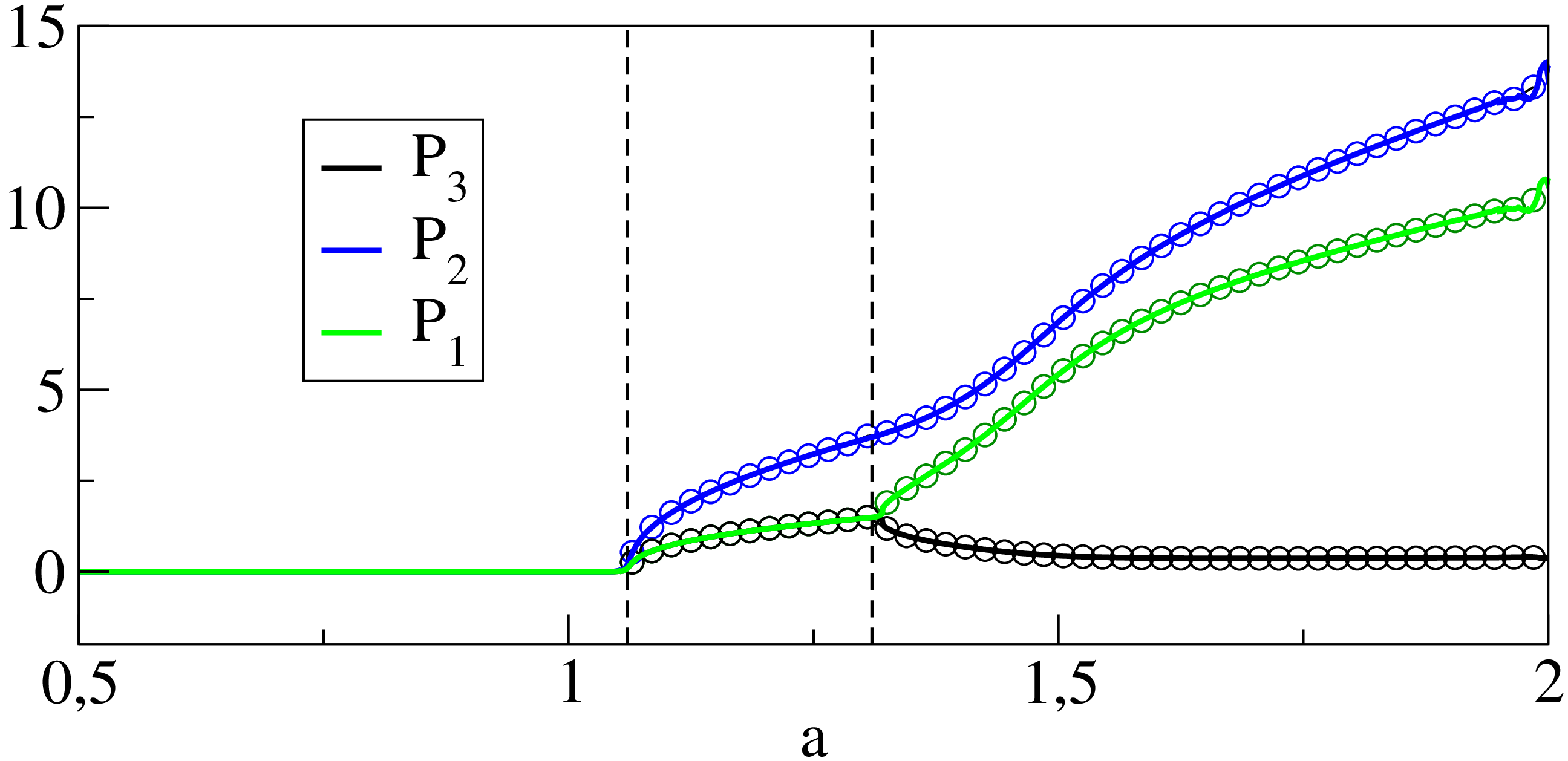
which gives the following eigenvalues: , and . Therefore, the origin is stable for and unstable for . For and this critical value is . This is shown also in Fig. 2, where the intensities in each waveguide is plotted, as a function of , while the other parameters and are kept fixed. The left dashed horizontal line marks the value where the origin loses its stability.
Beyond this point, the solutions are still stationary but nonzero and have the form (), where and are independent of the propagation distance. This ansatz leads to the following equations:
| (4) | |||||
| (5) | |||||
| (6) | |||||
| (7) | |||||
| (8) | |||||
| (9) |
where and , and therefore out of six real variables in the system of Eqs 1-3 we are left with five representing independent degrees of freedom.
From Fig. 2, we see that for the new stationary solution it holds that . In this case, the right hand sides of Eqs. 4 and 8 are equal. The same holds for Eqs. 5 and 9 and we therefore obtain:
| (10) | |||||
| (11) |
Multiplying Eq. 10 by and Eq. 11 by , subtracting them, and vice versa, we get that and . Therefore, given that Eqs. 4-9 reduce to the following system of five algebraic equations:
| (12) | |||||
| (13) | |||||
| (14) | |||||
| (15) | |||||
| (16) |
Solving Eqs. 13 and 15 with respect to , equating them, and using Eq. 16 we obtain:
| (17) | |||||
| (18) |
Moreover, from Eq. 13 we get that:
| (19) | |||||
| (20) |
Plugging this into Eq. 12 we can express as a function of , and by substituting it into Eq. 14 we finally obtain:
| (21) |
To ensure that the right hand side of this expression is positive, the signs of and must be chosen correctly. From Eqs. 13 and 15 it is easily found that is positive, therefore the valid sign in Eq. 17 is the “+” sign. With being positive, Eq. 21 requires that is also positive. To conclude, Eq. 21 (through 20) gives us the power in the first and third waveguide in dependence of the system parameters , and . This analytic solution together with the corresponding one for (given by Eq. 19), are shown with open circles in Fig. 2. The solid lines correspond to the solutions obtained via numerical integration of the initial system (Eqs. 1-3) using a standard fourth-order Runge-Kutta algorithm. The agreement is perfect. This special nonzero stationary solution is stable up to the value , marked by the right vertical dashed line in Fig. 2.
Beyond this critical point, it holds that and the analytical calculations become more complex. The solutions for are derived in the Appendix and are plotted with open circles in Fig. 2: We see that at a supercritical pitchfork bifurcation occurs and two new stationary solutions are born where and are interchangeable: when is on the lower solution branch, is on the higher solution branch, and vice versa. Finally, these two fixed points lose their stability in a Hopf bifurcation at and two periodic solutions take their place. All this will be discussed in the next section.
III Periodic solutions and Chaos
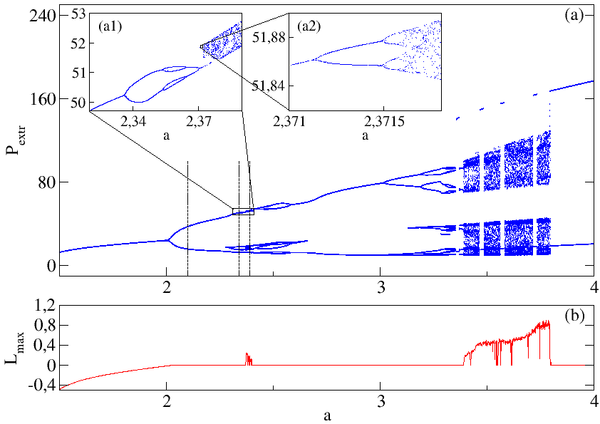
As we enter the regime of oscillatory solutions, the complexity of the system dynamics increases significantly. Figure 3(a) shows the orbit diagram in terms of the extrema , i. e. the maxima and minima, of the total power of light in the trimer over the imaginary part of the complex coupling coefficient for a fixed loss rate and coupling constant . The latter is kept constant throughout this section.
The orbit diagram has been produced via direct numerical integration of our model equations (Eqs. 13) and scanning of with a different random initial condition for each realization.
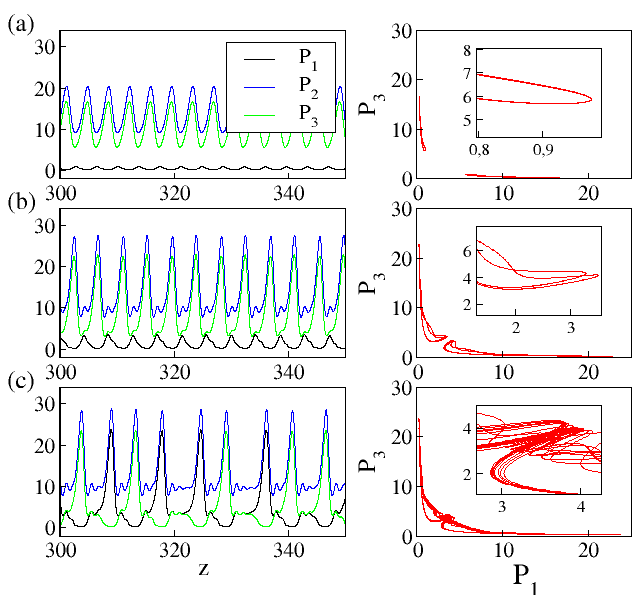
As we discussed in the previous section, initially the system’s stationary solution is a stable fixed point and the total power is constant. This fixed point loses its stability through a Hopf bifurcation at . Apart from its numerical evidence, the Hopf bifurcation has also been verified by applying a very powerful software tool that executes a root-finding algorithm for continuation of steady state solutions and bifurcation problems ENG02 . At the Hopf bifurcation, a limit cycle is born or, to be more accurate, two coexisting limit cycles are born, which are symmetric with respect to the diagonal in the () plane and are shown in Fig. 4(a).
The corresponding total power forms a single oscillatory solution which subsequently undergoes a period-doubling (PD) bifurcation in a thin region, which is blown-up in the inset (a1). The period-2 limit cycle that is born (shown in Fig. 4(b)) undergoes one more PD and subsequently a reverse PD bifurcation, forming thus a stable period-4 “bubble”. The latter is created (destroyed) through a period-doubling (reverse period-doubling) bifurcation at (). The appearance of bubbles BIE84 has been observed in several physical systems such as coupled superconducting oscillators HIZ18 .
Eventually, the system enters the chaotic regime through a period doubling cascade shown in the inset (a2). This scenario is repeated on a larger scale in a range of higher values, and a second wider chaotic regime, including windows of periodic motion within the chaotic attractor, can be observed in the interval . This self-similarity across different scales in the bifurcation pattern is a manifestation of the typical fractal structure of chaos, that we will address later on again.
Complementary to the orbit diagram, Fig. 3(b) shows the maximum Lyapunov exponent as a quantitative measure for characterizing the previously analyzed dynamical regimes. The maximum Lyapunov exponent has been calculated from the system equations of motion using the method described in WOL85 . As anticipated, there is a perfect agreement between Figs. 3 (a) and (b), i. .e. for negative the systems resides in a fixed point (flat , for the motion is periodic, while for the dynamics is chaotic. Concerning the latter, we observe that the Lyapunov exponents corresponding to the thin chaotic regime (around ) are much smaller than those of the wide chaotic region (), therefore implying weaker chaos in the former case.
As mentioned previously, at just after the Hopf bifurcation we have two limit cycles solutions which are symmetric for the two edge waveguides: Depending on the initial condition the intensity in the first waveguide is low, while the intensity in the third waveguide is high, and vice versa. Also, the edge waveguides are in anti-phase and the intensity in the middle waveguide is slightly higher compared to that in the edge waveguide. As the system undergoes the cascade of period and reverse period-doubling bifurcations the two symmetric limit cycles merge into one chaotic attractor (Fig. 4 (c)).
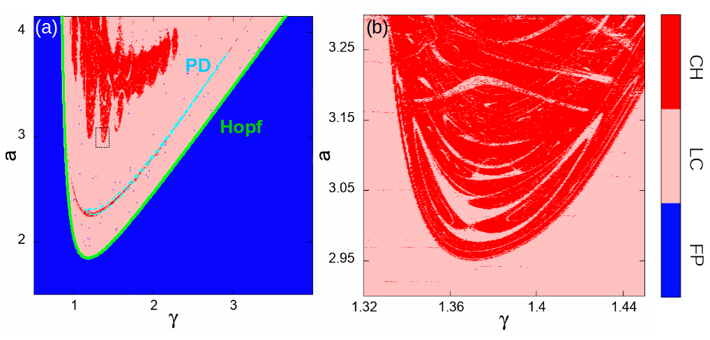
The dynamical scenarios described above are not specific to the selected value of and but rather extend to a wider range in the parameter space. For convenience we keep the coupling constant fixed and explore what happens in the plane. In Fig. 5(a) we classify the dynamics of the system based on calculations of the maximum Lyapunov exponent. Blue areas correspond to a negative and therefore to stationary solutions (fixed points “FP”), pink corresponds to a zero , i. .e periodic solutions (limit cycles “LC”), and red to a positive Lyapunov exponent , i. e. chaotic behavior (“CH”). The border between the blue and pink areas coincides with the Hopf bifurcation line which we have obtained via continuation ENG02 and have superimposed on the plot. Similarly, we have also included the first period-doubling bifurcation curve that marks the first transition toward chaos occurring in the system. Figure 5(b) shows a blow-up (marked by the dotted line rectangle) of Fig. 5(a), revealing the fractal-like structure of the chaotic regime that was discussed previously in the context of the orbit diagram Fig. 3(a).
IV Conclusions
We have studied in detail the nonlinear dynamical properties of an optical trimer with three lossy waveguides and complex coupling coefficients. The system supports stable stationary solutions, which are obtained analytically as a function of the underlying parameters of the problem, namely the loss, the real and imaginary (gain) parts of the coupling coefficient. In particular, in the oscillatory regime, the system exhibits two coexisting symmetric limit cycles that undergo a sequence of bubbles and period-doubling bifurcations leading to chaos. The calculation of the maximum Lyapunov exponent in the gain-loss parameter space reveals a fractal-like structure of the underlying dynamics. For future studies it would be interesting to study the -symmetric trimer in terms of chaotic behavior. Our preliminary results show that weak chaos is present bur further in-depth studies are required.
Acknowledgements
This project was funded by the European Research Council (ERC-Consolidator) under grant agreement No. 101045135 (Beyond Anderson).
V Appendix
Let us consider the general case for Eqs. 4–9 where . By setting , , , and , the system equations become:
| (22) | |||||
| (23) | |||||
| (24) | |||||
| (25) | |||||
| (26) | |||||
| (27) |
| (28) | |||||
| (29) |
Substituting Eqs. 28 and 29 into Eq. 25, we get as a function of :
| (30) |
while:
| (31) | |||||
| (32) |
Moreover, substituting Eqs. 28 and 29 into Eqs. 24 and 26, solving with respect to and equating both expressions we derive as follows:
| (33) |
Finally from Eq. 24 we find the following expression for :
| (34) |
All of the derived equations constitute parametric solutions with respect to , either directly (Eqs. 30, 31, 32), or through , , (Eq. 33) and (Eqs. 28, 29 and Eq. 34). Therefore by substituting them into one of the initial Eqs. 22–27, in principle we can find the solution of as a function of the system parameters (, and ). However, the calculations involved are extremely complex so we choose to do the following: We compute the value of as a function of via numerical integration of the initial system (Eqs. 1-3), we then calculate , and from the algebraic equations Eqs. 30, 31, 32 (we select the “+” sign in these expressions to ensure that ), and by plugging these values into Eq. 33 we obtain as a function of . Finally, from Eqs. 28 and 29, respectively, we also obtain and as functions of . These analytical values are shown with open circles in Fig. 2.
References
- (1) D. N. Christodoulides and R. I. Joseph, Discrete self-focusing in nonlinear arrays of coupled waveguides , Opt. Lett. 13, 784 (1988).
- (2) D. N. Christodoulides, F. Lederer, and Y. Silberberg, Discretizing light behaviour in linear and nonlinear waveguide lattices, Nature 424, 817–823 (2003).
- (3) S. M. Jensen, IEEE J. Quantum Electron, The nonlinear coherent coupler, 18, 1580 (1982).
- (4) N. Finlayson and G. L Stegeman, Spatial switching, instabilities, and chaos in a three‐waveguide nonlinear directional coupler, Appl. Phys. Lett. 56, 23 (1990).
- (5) J. C. Eilbeck, P.S. Lomdahl and A. C. Scott, The Discrete Self-Trapping Equation, Physica D 16, 318-338 (1985).
- (6) K.W. DeLong and J. Yumoto, Dynamics of the nonperiodic discrete self-trapping equation, Physica D 54, 36-42 (1991).
- (7) Y. Chen, A. W. Snyder, and D. N. Payne, Twin Core Nonlinear Couplers with Gain and Loss, IEEE J. Quant. Electron. 28, 239 (1992).
- (8) N. K. Efremidis and D. N. Christodoulides, Discrete Ginzburg-Landau solitons, Phys. Rev. E 67, 026606 (2003).
- (9) N. K. Efremidis, D. N. Christodoulides, and K. Hizanidis, Two-dimensional discrete Ginzburg-Landau solitons, Phys. Rev. A 76, 043839 (2007).
- (10) R. El-Ganainy, K. G. Makris, D. N. Christodoulides, and Z. H. Musslimani, Theory of coupled optical PT-symmetric structures, Opt. Lett. 32, 2632 (2007).
- (11) K. G. Makris, R. El-Ganainy, D. N. Christodoulides, and Z. H. Musslimani, Beam Dynamics in PT Symmetric Optical Lattices, Phys. Rev. Lett. 100, 103904 (2008).
- (12) Z. H. Musslimani, K. G. Makris, R. El-Ganainy, D. N. Christodoulides, Optical Solitons in PT Periodic Potentials, Phys. Rev. Lett. 100, 030402 (2008).
- (13) A. Guo, G. J. Salamo, D. Duchesne, R. Morandotti, M. Volatier-Ravat, V. Aimez, G. A. Siviloglou, and D. N. Christodoulides, Observation of PT-Symmetry Breaking in Complex Optical Potentials, Phys. Rev. Lett. 103, 093902 (2009).
- (14) C. E. Rüter, K. G. Makris, R. El-Ganainy, D. N. Christodoulides, M. Segev, and D. Kip, Observation of parity–time symmetry in optics, Nat. Phys. 6, 192 (2010).
- (15) K. G. Makris, R. El-Ganainy, D. N. Christodoulides, and Z. H. Musslimani, PT-symmetric optical lattices, Phys. Rev. A 81, 063807 (2010).
- (16) C. M. Bender and S. Boettcher, Real Spectra in Non-Hermitian Hamiltonians Having PT Symmetry, Phys. Rev. Lett. 80, 5243 (1998).
- (17) C. M. Bender, D. C. Brody, and H. F. Jones, Complex Extension of Quantum Mechanics, Phys. Rev. Lett. 89, 270401 (2002).
- (18) R. El-Ganainy, K. G. Makris, M. Khajavikhan, Z. H. Musslimani4, S. Rotter and D. N. Christodoulides, Nat. Phys. 14, 11 (2018).
- (19) Y. D. Chong, L. Ge, and A. D. Stone, PT-Symmetry Breaking and Laser-Absorber Modes in Optical Scattering Systems, Phys. Rev. Lett. 106, 093902 (2011).
- (20) P. Ambichl, K. G. Makris, L. Ge, Y. D. Chong, A. D. Stone, and S. Rotter, Breaking of PT Symmetry in Bounded and Unbounded Scattering Systems, Phys. Rev. X 3, 041030 (2013).
- (21) A. Regensburger, C. Bersch, M.-A. Miri, G. Onishchukov, D. N. Christodoulides, and U. Peschel, Parity–time synthetic photonic lattices, Nature 488, 167 (2012).
- (22) L. Feng, Y.-L. Xu, W. S. Fegadolli, M.-H. Lu, J. E. B. Oliveira, V. R. Almeida, Y.-F. Chen, and A. Scherer, Experimental demonstration of a unidirectional reflectionless parity-time metamaterial at optical frequencies, Nat. Mater. 12, 108 (2013).
- (23) B. Peng, S. K. Ozdemir, F. Lei, F. Monifi, M. Gianfreda, G. L. Long, S. Fan, F. Nori, C. M. Bender, and L. Yang, Parity–time-symmetric whispering-gallery microcavities, Nat. Phys. 10, 394 (2014).
- (24) H Hodaei, AU Hassan, S Wittek, H Garcia-Gracia, R El-Ganainy, D. N. Christodoulides, and M. Khajavikhan, Enhanced sensitivity at higher-order exceptional points, Nature 548, 187 (2017).
- (25) M.P. Hokmabadi, A. Schumer, D.N. Christodoulides, and M. Khajavikhan, Non-Hermitian ring laser gyroscopes with enhanced Sagnac sensitivity, Nature 576, 70 (2019).
- (26) K.G. Makris, I. Kresic, A. Brandstötter, and S. Rotter, Scattering-free channels of invisibility across non-Hermitian media, Optica 7, 619 (2020).
- (27) A. Steinfurth, I. Kresic, S. Weidemann, M. Kremer, K.G. Makris, M. Heinrich, S.Rotter, and A. Szameit, Observation of photonic constant-intensity waves and induced transparency in tailored non-Hermitian lattices, Science Advances 8, eabl7412 (2022).
- (28) K. G. Makris, Transient growth and dissipative exceptional points, Phys. Rev. E 104, 054218 (2021).
- (29) K. G. Makris, Transient amplification due to non-Hermitian interference of dissipative supermodes, Appl. Phys. Lett. 125, 011102 (2024).
- (30) I. Komis, D. Kaltsas, S. Xia, H. Buljan, Z. Chen, and K. G. Makris, Robustness versus sensitivity in non-Hermitian topological lattices probed by pseudospectra, Phys. Rev. Research 4, 043219 (2022).
- (31) H. Ramezani, T. Kottos, R. El-Ganainy, and D. N. Christodoulides Phys. Rev. A 82, 043803 (2010).
- (32) K. Li and P. G. Kevrekidis, Phys. Rev. E 83, 066608 (2011).
- (33) N. V. Alexeeva, I. V. Barashenkov, K. Rayanov, and S. Flach, Phys. Rev. A 89, 013848 (2014).
- (34) Y. Kominis, T. Bountis, and S. Flach, Scientific Reports 6, 33699 (2016).
- (35) L. Feng, Z. Jing Wong, R.-M. Ma, Y. Wang, and X. Zhang, Single-mode laser by parity-time symmetry breaking, Science 346, 972 (2014).
- (36) H. Hodaei, M.-A. Miri, M. Heinrich, D. N. Christodoulides, and M. Khajavikhan, Parity-time–symmetric microring lasers, Science 346,975 (2014).
- (37) B. Peng, S. K. Özdemir, S. Rotter, H. Yilmaz, M. Liertzer, F. Monifi, C. M. Bender, F. Nori, and L. Yang, Loss-induced suppression and revival of lasing, Science 346, 328 (2014).
- (38) S. Assawaworrarit, X. Yu, and S. Fan, Robust wireless power transfer using a nonlinear parity–time-symmetric circuit, Nature 546, 387 (2017).
- (39) J. Zhang, B. Peng, S.K. Özdemir, K. Pichler, D.O. Krimer, G. Zhao, F. Nori, Y. Liu, S. Rotter, and L. Yang, A phonon laser operating at an exceptional point, Nat. Phot. 12, 479 (2018).
- (40) H. Wang, Y. H. Lai, Z. Yuan, M.G. Suh, and K. Vahala, Petermann-factor sensitivity limit near an exceptional point in a Brillouin ring laser gyroscope, Nat. Comm. 11, 1 (2020).
- (41) S. Xia, D. Kaltsas, D. Song, I. Komis, J. Xu, A. Szameit, H. Buljan, K.G. Makris, and Z. Chen, ”Nonlinear tuning of PT symmetry and non-Hermitian topological states”, Science 372 , 72-76 (2021).
- (42) Y. G. N. Liu, Y. Wei, O. Hemmatyar, G. G. Pyrialakos, P. S. Jung, D. N. Christodoulides, and M. Khajavikhan, Complex skin modes in non-Hermitian coupled laser arrays, Light Sci. Appl. 11, 1 (2022).
- (43) I. Komis, Z.H. Musslimani, and K.G. Makris, Skin solitons, Opt. Lett. 48, 6525 (2023).
- (44) K. Engelborghs, T. Luzyanina, and D. Roose, ACM Trans. Math. Software 28, 1 (2002).
- (45) M. Bier and T. C. Bountis, Phys. Lett. 104, 239 (1984).
- (46) J. Hizanidis, N. Lazarides, and G. P. Tsironis, Chaos 28, 063117 (2018).
- (47) A. Wolf, J. B. Swift, H. L. Swinney, and J. A. Vastano, Phys. D 16, 285 (1985).