A local diagnostic program for unitary evolution in general space-times
Abstract
We present a local framework for investigating non-unitary evolution groups pertinent to effective field theories in general semi-classical spacetimes. Our approach is based on a rigorous local stability analysis of the algebra of observables and solely employs geometric concepts in the functional representation of quantum field theory. In this representation, it is possible to construct infinitely many self-adjoint extensions of the canonical momentum field at the kinematic level, and by the usual functional calculus arguments this holds for the Hamiltonian, as well. However, these self-adjoint domains have only the trivial wave functional in common with the solution space of the functional Schrödinger equation. This is related to the existence of boundaries in configuration field space which can be penetrated by the probability flux, causing probability to leak into regions in configuration field space that require a more fundamental description. As a consequence the evolution admits no unitary representation. Instead, in the absence of ghosts, the evolution is represented by contractive semi-groups in the semiclassical approximation. This allows to quantify the unitarity loss and, in turn, to assess the quality of the semi-classical approximation. We perform numerical experiments based on our formal investigations to determine regions in cosmological spacetimes where the semiclassical approximation breaks down for free quantum fields.
I Introduction
Once quantum fluctuations of spacetime are excited, the semiclassical approximation for quantum fields in curved spacetimes implies a non-unitary evolution, because the approximation assumes an inert classical motion for the background geometry [1, 2, 3, 4, 5]. Unitarity violations are concomitant with sources or sinks for probabilities. Assuming the quantum theory is consistent (in Minkowski spacetime), sources violating probability conservation cannot exist while probability sinks are allowed, implying that the spectrum of the Hamiltonian contains eigenvalues with a negative imaginary part. This can be interpreted as a measure of the extent to which the semiclassical approximation is invalidated. Of course, probability sinks have only operational consequences, provided that they involve detectable unitarity violations, which, in turn, translate into the breakdown of the semiclassical description.
The corresponding evolution operators are a contractive representation of the time translation group. In the spirit of Stone’s theorem, which establishes a one-to-one correspondence between self-adjoint operators and certain one-parameter unitary groups, contractive representations enjoy accretive generators [6]. While this grants the semiclassical approximation predictive power and is a nice feature at the technical level, it also qualifies the underlying Hamiltonian as non-observable if regions of spacetime are considered that contain probability sinks.
Any description of a system in curved spacetimes within the semiclassical framework can, therefore, at best be an effective field theory [7]. This holds, in particular, for free quantum fields coupled to dynamical background geometries that are assumed to be inert against quantum fluctuations. This assumption might be violated in spacetime regions which support fluctuations of observables that violate the corresponding mean field. At the operational level, any observer must single out a set (algebra) of observables which they intend to measure in certain regions of spacetime. Statements concerning stability can only be made relative to this set. The validity of the semiclassical approximation depends on the probability to excite quanta beyond a boundary in field configuration space. The boundary field configuration relates to a geometric argument based on semi-norms concerning the stability of background observables.
The existence of such a boundary is crucial as there are no asymptotic conditions imposed on the domains of the functional integrals and, instead, observables have to be evaluated on finite boundaries. The boundary field configurations also impact the spectral analysis of field operators. As we show in the main body of the text, the canonical pair consisting of a real scalar field and its conjugated momentum field enjoy self-adjoint extensions on certain Hilbert spaces, hence they constitute the basic observables. However, the notion of basic observables is only meaningful at the kinematical level: the solution space of Schrödinger wave functionals might not intersect the Hilbert space on which the canonical pair admits a self-adjoint realization. From this point of view, quantisation (of polynomial observables) clashes with the dynamical content of the theory.
The functional Schrödinger picture of quantum field theory (cf. [8, 9, 10, 11, 12, 13, 14, 15, 16, 17, 18, 19, 20, 21, 22, 23, 24, 25, 26, 27] for details) allows to address the questions raised above, in particular, to determine the domain of validity associated with the semiclassical approximation and its concomitant unitarity violation. In the absence of ghosts, unitarity violation is tied to a significant probability flux across the boundary in field configuration space. Whether the violation of probability conservation is acceptable depends on the resolution with which observables are measured. If unitarity violations are acceptable within the spacetime region associated with the measurement process, then contractive representations generalize unitary evolution groups and grant predictive power even when the probabilistic framework underlying effective quantum theories becomes challenged.
The formal arguments presented in the main body of the text are applied to simulations employing Gaussian random fields. Based on these numerical experiments, we demonstrate the potential of the formalism by studying free fields in cosmological spacetimes, such as contracting radiation dominated universes evolving towards a future singularity and the asymptotic past of de Sitter universes. The simulations reveal regions in these spacetimes, where the semiclassical approximation fails relative to a geometric stability criterion on the algebra of observables.
The article is organized as follows: In Sec. II.1 the kinematic aspects of effective field theories in curved spacetime are discussed in the Schrödinger representation, including preliminaries and new topics such as effective configuration field spaces and stability analysis based on geometric and functional methods, spectral properties of functional operators in the presence of configuration field boundaries, the impact of these boundaries on self-adjoint extensions of the functional momentum operator and the functional Hamilton operator at the kinematic level. Sec. III confronts the results obtained in the previous section with dynamic aspects. The following Sec. deepens the preceding discussion and takes a fresh look at contractive evolution semi-groups. This concludes the formal considerations of the article. In Sec. V we apply our formal results to study effective field theories in cosmological spacetimes and domains of validity of the semiclassical approximation by employing numerical experiments. The conclusion of the present work is presented in Sec. VI and followed by two appendices, App. A and B, concerning the notation employed in this article and some technical aspects of the numerical experiments.
II Kinematic Aspects
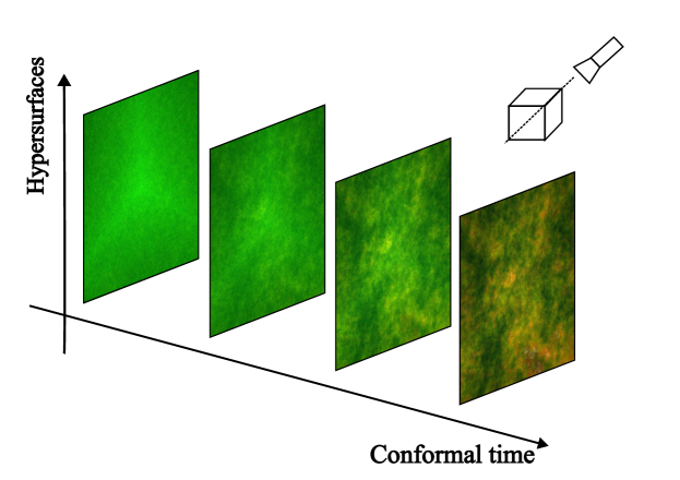
In this section, we provide a brief overview on the kinematic aspects of the functional Schrödinger representation in quantum field theory. For simplicity, we consider only globally hyperbolic spacetimes , where is a connected four-dimensional, smooth, Hausdorff manifold, and is a Lorentzian metric. The manifold is diffeomorphic to with [28], and it foliates into hypersurfaces . Relative to this foliation, the metric is given by
| (1) |
where denotes the lapse function, the dual shift vector, and is a Riemannian metric on .
For , let be a real vector bundle over the hypersurface , given by the quadruple , where denotes the total space, is the bundle projection of onto the base , and is a real vector space homeomorphic to the fibre . In the following, we consider only trivial bundles of rank one over and refer to as the configuration bundle of instantaneous field configurations. Configuration fields are smooth sections of , collected in the vector space . Of particular interest is the space of compactly supported smooth sections of the configuration bundle .
Let denote a formal measure space. Consider the complex vector space of measurable complex-valued wave functionals in , whose modulus is square integrable with respect to the formal Lebesgue measure . Let be the subspace consisting of wave functionals that vanish -almost everywhere. The quotient space can be equipped with a norm , where
| (2) |
for any bounded operator on . Note that while is a formal norm on , it is merely a semi-norm on .
Concerning the underlying probabilistic framework (refraining from topological issues): if is a measurable subset of , let denote the functional , then is the probability for the instantaneous configuration fields in to populate the hypersurface . The brackets denote the inner product associated with . This interpretation assumes that has been normalized to unity on the initial hypersurface.
The first elementary observable we consider is the smeared configuration field operator , where is an instantaneous field configuration of compact support, . The domain of is given by all wave functionals in such that is in for all admissible smearing functions. For wave functionals in this domain, . In other words, the smeared configuration field operator acts as a multiplication operator on its domain in . A measure for the probabilistic scatter of instantaneous configuration fields around the expectation value with respect to the wave functional is .
The second elementary observable, the smeared momentum field operator conjugated to is defined as the functional generalization of a directional derivative111Let be a test function of compact support, the functional derivative can be thought of as a generalized directional derivative where the generalization to multiple applications of follows immediately [29]. such that the canonical commutation relation holds. We refrain from giving a precise characterization of the domain of for now, but it certainly encompasses those wave functionals in with for all smooth smearing functions of compact support on . The matter of the domain will be the subject of a later discussion in Sec. II.3. The canonical commutation relations imply Heisenberg’s uncertainty relation. From these elementary observables others can be formed using a natural generalization of functional calculus as characterized in the spectral theorems of unbounded operators.
This concludes our brief review of the kinematic aspects underlying the Schrödinger picture of quantum field theory in Lorentzian spacetimes.
II.1 Effective Configuration Spaces
So far we considered formal measure spaces with in some interval as configuration spaces and wave functionals in the dual vector bundle satisfying . Clearly, contains some field configurations that are inadmissible for a semi-classical treatment. Therefore, in this section, we construct an admissible configuration space.
In classical field theory, a local observable is a smooth section in such that for each background configuration there exists a neighborhood in in which for all fluctuations relative to in we have , where denotes the jet prolongation of at , and is a functional on the jet bundle , where . Note that we hide any dependence on the background geometry for the ease of notation. The canonical quantization prescription allows to map any local observable to a (bounded) operator on , denoted by the same symbol for simplicity. Note that the definition of local observables in classical field theory is adapted to a covariant framework, while the quantization prescription in the functional Schrödinger picture requires a foliation of spacetime into hypersurfaces222 From this perspective it might have been more appealing to consider local functionals on the momentum phase space of a given classical field theory. We refrain to follow this logic in order to keep the presentation concise. .
In the following, we assume that the background configuration is in , where is the hyperbolic wave operator associated with the free theory.
We choose a set of finitely many local quantum observables with support in . Our first objective is to characterize further. Any quantum observable in can be represented as in , where denotes the corresponding classical observable evaluated at the background configuration. Let denote the length dimension of , and let be a short-distance cut-off below which a fundamental description is eventually required333 In fact, there might be an ordered set of cut-offs such that the description of a finite number of observables in the effective theory with cut-off is contained in the description labeled with cut-off .. We consider as the short-distance limit of the quantity corresponding to , which allows to introduce the dimensionless ratio
| (3) |
Given a wave functional , we introduce the filtering semi-norm
| (4) |
where ; for any background configuration , in the interval , and require
| (5) |
for any sensible fluctuation. If denotes the length scale characterizing , then scales as for either sign of . Any observable in violating this bound requires a description characterized by a short-distance cut-off , including . Unless (5) is violated, one describes a theory that is consistent with any length scales, provided its existence. In this sense, is the largest neighborhood of that complies with the criteria (5).
Suppose it is possible to contract the neighborhood of sufficiently to comply with (5), then can be described by an effective field theory with a short-distance cut-off beyond which a more fundamental theory is required.
This, however, does not imply that admissible fluctuations respect the background configuration. Relative to , the background seems stable provided that
| (6) |
where is assumed to be in the open interval . The value is excluded since it corresponds to a trivial fluctuation relative to , and is excluded since it corresponds to fluctuations that equalize the background observable with respect to some quantum observable included in . Such fluctuations will trigger non-negligible backreactions on the classical observable. In this sense, has the meaning of a resolution scale relative to and quantifies to which extent the background configuration can be distinguished from fluctuations based on the local quantum observables in if the system is in a state represented by the wave functional . It is possible to develop this interpretation further by considering actual measurement processes, but we leave this for future work. Note that only the concept of background stability relative to a chosen set of local quantum observables is sensible. Relative background stability might imply a further contraction of .
The contractions of entailed by (5) and (6) guarantee a faithful description of those fluctuations respecting the background configuration within the framework of effective field theories at the level of local quantum observables contained in . We will always assume that has been contracted accordingly and denote the restriction of the formal measure space in accordance with the consistency conditions (5) and (6) by . Accordingly, marks the range of validity for the considered effective framework.
At last, we emphasize that our criterion in (6) is general: the choice of should not be seen as limited to quantities derived solely from the classical field 444 For example, in the case of a free quantum field, a comparison with classical observables based on classical fields is meaningless, as one can find a trivial background, i.e., .. The comparison between and is meaningful only when it aligns with the specific questions being addressed. Suppose we are concerned with the stability of the classical spacetime geometry. In this case, the appropriate quantities to compare will involve the expectation value of the Hamilton operator for a given quantum state, relative to geometric quantities that determine the energy scale of the curvature. Examples are the black hole mass in Schwarzschild spacetimes, or the square of the Hubble parameter in FLRW spacetimes.
II.2 Analysis of Operators
In this section we prepare the spectral analysis [30, 6, 31] of various functional operators. This analysis requires to introduce smooth approximations of the identity in and is limited to an important subset of multilocal functions, given below, including Gaussian states. This limitation does not correspond to a mathematical requirement, it is rather a convenience for explicit computations.
Let denote a subset of in accordance with the conditions (5) and (6), consisting of fluctuations around a stable background in the domain of some effective field theory. The hypersurfaces parameterize the sections of the real line bundles at any permissible time, and is bounded by two sections and in which comprise its geometric boundary relative to along . In other words, for , at any point in the hypersurface . For better readability we refrain from specifying boundaries by their respective base manifolds.
We introduce the one parameter family of approximate identities as follows: let with support contained in so that its integral over equals to one. On each fiber , this family is given by the usual family of Dirac distributions in . The relation between the global and local versions is .
In this article, we focus on a trivial but important subset of so-called multilocal functionals:
| (7) |
where is a complex valued functional in , and it is understood that is a complex number. This subset is trivial in the sense that each copy of the jet expansion of the configuration field terminates at the lowest order contribution. And it is important since it contains Gaussian states: Choose , and for ,
where . Let be the evaluation functional returning the value of its argument at , and let denote its dual. We expand
| (8) |
and find by direct computation
| (9) |
for a suitable configuration space.
Let be a multilocal functional of the form (7) on . For , consider the one parameter family of functionals
| (10) |
We compare both functionals and :
where the supremum is taken over . The first estimate follows from the triangle inequality and the properties of the approximate identity, and the second from the definition of the supremum as the least upper bound estimate. Again, this inequality uses properties of the approximate identity. Whenever , is required to approximate to an ever better degree. As a consequence, the right hand side of the above inequality converges to zero and, therefore, in .
In the remainder of this section, we highlight informally some construction of functional differential operators. At this stage, the discussion is kept at a formal level without considering questions pertinent to infinite dimensional analysis including, in particular, domain questions. These will be settled in Sec. II.3 that is devoted to a thorough analysis of the functional momentum operator and its spectral properties.
Let , the functional differential is characterized by
| (11) |
for all , which is a convenient way to store all the functional derivatives of multilocal functionals. In the exceptional case of a local functional, the functional differential is given by exchanging the argument of the functional with the direction of the functional derivative, .
The functional gradient of a multilocal functional is the multilocal functional . In DeWitt’s condensed notation [32],
| (12) |
The functional Hessian is its second functional differential . In greater detail,
| (13) |
The functional Laplacian is the contraction which for a bi-local functional yields for some function .
II.3 Functional momentum operator
In this section we present the spectral analysis of the functional momentum operator on domains subject to boundaries in configuration field space.
We proceed in three steps. The first is of pedagogical nature and prepares us for the proof that extends , where denotes the closure of with domain and is defined on the domain . Again, denotes the compactum in the space of instantaneous field configuration in accordance with (5) and (6). As a consequence, these domains require to specify conditions on the boundary .
In the next step, we show that is symmetric on a certain pre-Hilbert space and determine its adjoint on a related, but less restrictive, pre-Hilbert space. It remains to argue that these pre-Hilbert spaces are, in fact, complete with respect to the norm induced by the inner product. Finally, we derive that is not essentially self-adjoint and classify all self-adjoint extensions. Since the functional momentum operator is so simple, this can be done by direct computation instead of employing von Neumann’s deficiency indices [30].
Without going right away into details about the domain of the functional momentum operator, it certainly encompasses . So for the moment, let and , be subjected to boundary conditions on . It is useful to work with the functional generalization of directional derivatives: for , let
| (14) |
where denotes the functional derivative in the tangent space to the fiber located over in field configuration space, if , and accordingly for . Note that the functional derivative includes a factor evaluated at . Since the induced volume factor is smooth, it can be absorbed in .
The approximate identity constructed above is by assumption in , so we can evaluate on the one-parameter family of functionals :
In order to comply with conditions (5) and (6), the boundary term is required to vanish, which restricts the domain of further. Explicitly,
Our previous discussion following (10) demonstrated that since has support on a fixed compact subset in the space of instantaneous field configurations, in , and now we find similarly that in , as . This shows that the closure of contains .
To determine the adjoint of , we introduce below the notion of absolute continuous functionals. Consider the formal measure space and for each , define to be the collection of all countable families of pairwise disjoint open connected sets with , where denotes the finite volume of . We call a functional absolutely continuous if for every there is a so that for any we have
| (15) |
We denote the set of all absolutely continuous functionals on with values in by . The subset of all bounded functionals in is an algebra over .
Let and, as before, . The functional momentum operator is densely defined and an integration by parts shows that it is symmetric. Let . Then, by definition, the adjoint satisfies [30, 6]
| (16) |
where and is a smooth approximation of the indicator functional, which is locally characterized by if for every , and zero otherwise. The right hand side of (16) is readily computed:
| (17) |
The left hand side of (16) requires more work.
| (18) | |||||
The first term on the right hand side of this equation vanishes since by construction. In the limit equation (16) becomes
| (19) |
So fiberwise we have
| (20) |
which means is absolutely continuous, , and . The other direction is similar: integration by parts shows that any is in the domain of and for . Therefore and .
Clearly, . Moreover, is not essentially self-adjoint. Just consider [33]
| (21) |
where is a real valued functional on the compactly supported smooth sections of the configuration bundle , and .
This raises the question whether has any self-adjoint extensions. The answer, given below, is positive and constructive since it provides a complete classification of all self-adjoint extensions. Let be the operator on with the domain . We showed above that is symmetric on this domain and that the adjoint is the operator with domain . For and consider the difference
| (22) |
Since we perform an integration by parts in the second term and find
| (23) |
where with the following sign convention implied: . For a self-adjoint extension is necessarily required to be zero, which is precisely enforced by the boundary conditions specified in the domain of the functional momentum operator. Note that this holds without imposing any boundary conditions on those wave functionals in the domain of the corresponding adjoint operator. Therefore, the functional momentum operator defined this way is not self-adjoint.
Assume there exists a self-adjoint extension of and choose a . Then (23) demands that
| (24) |
where . For , let
| (25) |
Since by assumption , equation (23) can become zero if and only if there exists a complex valued function on with unit modulus so that
| (26) |
is true at any point on the hypersurface . This condition is required to hold for any functional in with the same function . Introduce on
| (27) |
Clearly . Since is symmetric and is by assumption a self-adjoint extension of , we have for some function with .
It remains to determine which of the symmetric extensions are in fact self-adjoint. Let and . Then (23) being zero requires
| (28) |
at every point in the hypersurface , which locally has the following solution: . But then , and we are safe to conclude . In other words, all symmetric extensions , indexed by a complex valued function on with unit modulus, are self-adjoint. Apparently we have found infinitely many self-adjoint extensions which describe different physics [6]. Of course, this is to be expected from the point particle limit.
In the following section, we will extend our analysis to find the self-adjoint domain of the Hamilton operator. This will bring us one step closer to studying the consequences of the dynamics it generates.
II.4 Hamilton Operator
As a proof of concepts, it is sufficient to consider the Hamiltonian of a free field. The operator of interest is therefore the functional generalization of the Laplacian introduced above at the informal level. Discussing the spectral properties of the functional Laplacian is an application of quadratic form techniques and positivity based on a theorem by von Neumann which was originally proven [6] using operator-theoretic techniques in the case of point particles.
Let be a quadratic form on the form domain , defined by , so that is conjugate linear and is linear for . Apparently, is nonnegative and since is closed as an operator, is closed as a quadratic form. Then there is a unique self-adjoint operator associated with . This follows from the Riesz lemma, the Hellinger-Toeplitz theorem, and by direct application of the spectral theorem in multiplication operator form. We will now determine the operator that is associated with the kinetic part of the Hamilton operator.
Note that is a subspace of the Hilbert space under the inner product . Denote by the space of bounded conjugate linear functionals on . Introduce the linear embedding of into by . From the Cauchy-Schwarz inequality it follows that this map is bounded. Since the identity map embeds in , we have the following chain of inclusions: Define by . From the definition of the formal adjoint we see that and equals restricted to . Next, let be the map given by . The proof of the theorem associating a (unique) self-adjoint operator to a closed positive quadratic form mentioned above gives and equals restricted to . Let . Then . Hence, . Therefore,
| (29) | |||||
where the first equality is just the quoted result on the domain of , the second equality follows from , and the third and fourth are straightforward. Moreover, equals restricted to the domain of which equals . In other words, the self-adjoint operator associated with the closed positive quadratic form is .
Hence, we are ultimately equipped to determine the solutions to the functional Schrödinger equation for a free quantum field theory which we will then compare with the self-adjoint domain.
III Dynamical aspects
Our previous discussion showed that in a configuration field space subjected to boundaries at a finite distance, it is always possible to construct a momentum operator and its quadratic form with infinitely many self-adjoint extensions on a kinematic level. This mere possibility does not necessarily imply compatibility with the dynamics imposed by the Schrödinger equation for any .
In this section, we present the dynamic analysis to accompany the kinematic statements. We proceed in three steps: first, we investigate, for Gaussian wave-functionals, under which criterion the Hamilton operator admits a self-adjoint extension on the kinematic level. Second, we introduce the dynamics provided by the functional Schrödinger equation and examine the corresponding solution space . Third, we show that only static space-times provide the possibility for such self-adjoint extensions that are respected by the dynamics.
We begin with determining the self-adjoint domain of a Gaussian state in . Consider where is given by (9) and denotes the normalization we will determine later. Then, demands
| (30) |
where , means that is evaluated at the boundary , which sets . The functional integral is given by a consistency requirement that cannot be a functional of for all . Note that, while the condition (30) holds true when for all , this only reflects the trivial choice of a set containing only a single point, i.e. .
Suppose for all . Then, the functional integral remains parity even, i.e. for all the map will not modify the integral in (30). The important difference, however, is located in . Since
| (31) | ||||
then for all , sending yields
| (32) |
which concludes that and can be satisfied, provided that for all . Accordingly, there exist infinitely many self-adjoint extensions of provided that
| (33) |
An immediate follow-up question would be whether or not the Hamilton operator for a free scalar field admits similar extensions. The answer to this question is in the positive and is mainly concerned with the spectrum of the kinetic operator . For to be self-adjoint, must hold for any where admits a unit modulus. This results in the following two relations coming from and (26)
| (34) | |||
| (35) |
which provide two conditions under which admits self-adjoint extensions. Since is Gaussian, (34) can be re-expressed as
where . Using (26), the above equation reduces to
| (36) |
Evaluating the functional derivative explicitly yields
| (37) | ||||
When inserted into (36), admits self-adjoint extensions if the following equation holds true:
| (38) |
Since is not a valid element of the Hilbert space , this indicates that either or . The first derived condition violates in general (III) unless there exists a for which . From the second condition we have which imply that cannot be an element of in static [9] nor dynamical spacetimes.
Since (34) covers only trivial solutions, we focus on (35) instead. Using , we reduce (35) to
| (39) | ||||
where we have considered and limited ourselves to which excludes .
By the same consistency requirement that cannot be a functional of for all , we integrate out all the dependency in (39) with . To condense the necessary requirement for self-adjoint extensions we multiply both sides with before we integrate over for all . Given that , one finds
| (40) |
As such we are left with the necessary condition
| (41) |
which suggests either the criterion Im for all or . If instead and , we conclude . This can be met if either is compact, such that , or is non-compact, such that the asymptotic fall-off conditions for guarantee . However, we are in neither case because is Gaussian and is compact. We are left with for all . Thus this is the criterion for to admit self-adjoint extensions.
The subsequent spectral analysis immediately trickles down to the Hamilton operator. Let a Gaussian wave-functional, its most general form is as in (9) with . For to be associated with physical systems, is a solution to the functional Schrödinger equation
| (42) |
where is defined as in Section II. Adopting the foliation (1), the Hamilton operator decomposes into where and where the individual terms are [11, 10]:
| (43) | ||||
where is defined as in (29), the Laplace operator with metric induced on . For is the coupling parameter to the Ricci scalar curvature , we assume that the operator acting on yields real eigenvalues, such that the self-adjointness of passes on to . The off-diagonal part is not particularly important because it can be eliminated by a (local) coordinate transformation to diagonalize the Hamilton operator. What would always remain, is the diagonal part of , that is .
As a result, to conclude our analysis for , we are required to concern only , which implies to determine whether or not admits self-adjoint extensions. To this aim we show that for a general satisfying (42), features complex functionals of if the space-time is dynamical, such that cannot admit any self-adjoint extension, although they exist for . Let us sketch the solution space determined by (42) for a free scalar field theory on a dynamical, globally hyperbolic space-time. For the Gaussian state we find the following two equations to be satisfied by
| (44) | ||||
| (45) |
where . All that solve the above equations span . It is obvious that any space-time dependence comes from the metric which is implicitly contained in , , , etc. Now we show that these elements are incompatible with the self-adjoint domain of , Dom, by contradiction. Recall, the self-adjoint domain requires Im, consider now the generic solution to (45) in local description [11]
| (46) |
where denotes the integration constant of the -integral. Suppose for all , then . Since , admits a self-adjoint extension which ensures norm conservation . By direct computation, we find
| (47) |
This identity is true for all , if and only if for , or otherwise (47) is false. The former requirement is possible only if the kernel is time independent which is tantamount to saying that the space-time is static. In this case, (42) reduces to the time independent Schrödinger equation for [9]. If, however, the space-time is dynamical, then implies that by consistency it is impossible to meet such that the Hamilton operator has a self-adjoint extension. On the contrary, when a space-time is static, for example, Minkowski space-time, then it is clearly possible for to admit infinitely many self-adjoint extensions whilst .
IV Contractive Evolutions
Until now, we only considered the spectrum of which eventually generates the time-evolution operator. As shown in the previous section, is not necessarily essentially self-adjoint. Here, we delve deeper into the implications and consequences for the evolution group. This allows us to morph Stone’s pair in quantum mechanics (essentially self-adjoint Hamilton operator unitary evolution group) into a generalized, functional version.
For reasons that will soon become clear, we consider a one-parameter family of evolution operators on (with denoting the initial configuration space at time ) satisfying , the map is continuous for each initial wave functional in and . Moreover, we consider only a special family of evolution operators, called contractive [6], which satisfy the additional condition
Contractive evolution families arise naturally in effective field theories and provide a necessary generalization of the relationship between unitary evolution groups and self-adjoint generators of time translations.
As in the case of contracting evolution semigroups (including unitary representations of evolution groups), we obtain the generator of for as follows: Introduce555Of course, will be the Hamilton operator but since this is a more general analysis, we decided to rename the generator for time translations. and consider the domain for the infinitesimal generator , defined by for all in . We will also say that generates and write the time-ordered exponential
| (48) |
Note that is dense in : consider any in , and set
| (49) |
for . Here, the idea is that the sequence converges to as approaches zero. If is in for any and for each , then any is the limit of a sequence in , and, thus, would be dense in . Now, for any such that , consider . We can rewrite as , because the evolution operator reduces to an ordinary exponential describing time-translation when it is applied to a solution of the evolution equation . Hence,
| (50) | |||||
So for each in and for each admissible , the sequence lies indeed in , and, therefore, is dense in . It is worth stressing that the evolution equation is required in this derivation since, in general, the dynamical content of the theory is given by a one-parameter family of time-ordered exponentials which does not even constitute a semi-group. However, if is in the domain of , then , so , and .
We can use this to show that is also closed: Let be a sequence of wave functionals in converging to in , and . Then . Integrating the evolution equation gives , where has been used (since the sequence is by assumption in the domain of ). Thus, . The limit is . For , we find , so and . Since is closed, this allows to perform a generalized spectral analysis which is essential to relax the description of Stone’s pair. Now we turn our attention to the necessary property that is attributed to the generator.
IV.1 Accretive generators
We proceed with considering contracting evolution operators and remind the reader that they are a (necessary) generalization of unitary evolution operators. While the contraction property replaces unitarity, it remains to investigate what supplants self-adjointness as the related property of the infinitesimal generators.
Let be in the spectrum of the infinitesimal generator , (for simplicity). Introduce and . Consider the formal Laplace transform666Considering a one-sided exponential decay multiplied by a Heaviside distribution which resembles a contracting semi-group evolution. The corresponding Laplace transform yields .
| (51) |
Assume that . Then, if , and since by assumption, is a bounded linear operator of norm less or equal to . For positive ,
| (52) | |||
where the second equality holds after shifting in the second Laplace transform, and . In the limit , we find . Hence, and . This implies . Furthermore, for , we have , so on since and are integrable by the condition on the spectrum of , and the fact that is closed. As a consequence, for , the following holds: , which implies that holds in the strong sense.
Apart from the restrictive adaption to include time-ordered exponentials as evolution operators, the above reasoning follows the proof of the necessity part of the Hille-Yosida theorem [6]. The spectral properties of are also sufficient to guarantee a contracting family of evolution operators: let be real positive and introduce on . The derivation proceeds in three steps: first, we will prove that as for any wave functional in . Then we will show that the semigroups are contracting and construct as the strong limit of these semigroups.
For in , we have . Moreover, from the necessity part discussed above, for all real positive , so
since by the above bound. It follows that the family is uniformly bounded in norm, so for all in , given that is dense in this space. Hence, as .
The semigroups with infinitesimal generators are defined by power series. Since
where the first equality is due to the definition of , the first equality follows from the triangle inequality and the last from the bound on , because they are contracting semigroups. Let be real positive, and . Then
Using that is a commuting family of infinitesimal generators,
The last inequality follows from the contraction property of the semigroups generated by . Since we have shown above that converges to as , is a Cauchy sequence in this limit for any real positive and in . Let us set , since the properties of contraction semigroups are preserved under strong limits, constitutes a semigroup of contracting evolution operators. The above inequality shows that is a strongly continuous contraction semigroup.
Let be the infinitesimal generator of . For all and ,
and therefore
since converges to in the limit . Now, in the limit , the left-hand side converges to and the right-hand side to . Thus converges to . Therefore and restricted to the domain agrees with . It remains to show that both domains coincide. For real positive , the inverse of exists by the necessity part of the statement shown above, and the inverse of exists by hypothesis. Hence, , and, as well, , so indeed .
The above derivation requires to construct the resolvent of the infinitesimal generator of the evolution operator in order to verify the spectral properties that are necessary and sufficient to generate a one-parameter family of contracting evolution operators. If is in the domain of for , then the contraction property implies within Dom
| (53) |
Therefore, the contraction property requires that Re is semi-positive definite. Such a densely defined infinitesimal generator is called accretive.
By identifying the infinitesimal generator with the Hamilton operator , we can link this with the previous discussion. Albeit being complex-valued, if the spectrum admits a suitable sign in the imaginary (or real part), the evolution can be described by evolution operators that keep the probabilistic feature of the theory intact [17, 19]. In the spirit of Stone’s theorem we see that one-parameter families of evolution operators admit in general contracting representations generated by accretive operators. This includes the celebrated situations that allow for a unitary evolution generated by self-adjoint operators which are formal observables of the theory [34].
IV.2 Initial data
In sections III, IV.1, statements concerning the dynamical content of the theory have been derived assuming time-evolved data as input. Consequently these statements do not extend to wave functionals on Cauchy hypersurfaces. The goal of this section is to close this loophole.
For simplicity, let be a half-open, left-closed interval of the extended real numbers with denoting its minimum element, and with being an arbitrary small positive number such that is continuous on and smooth on the interior of . Consider the integrated evolution equation
| (54) |
The mean value theorem for definite integrals guarantees that there is a real number in the interior of such that . We can write with . Since is a positive fraction of , it follows that , where is in the interior of arbitrary close to the minimum element of , and is the Bachmann-Landau notation to denote the order of approximation. This can be seen as follows: by iteration of the integrated evolution equation, , where the given order of approximation refers to the product with each factor parameterizing the numbers guaranteed by the mean value theorem. In the limit , we find . Since is a strictly decreasing sequence (again by the mean value theorem), the definition of the time-ordered evolution operator shows that the above result holds to arbitrary precision. The infinitesimal evolution operator is (at linear order in small quantities) a member of a one-parameter family of strongly continuous semigroups: the existence of an identity is obvious, the composition law holds at linear level and the continuity property by hypothesis.
V Cosmological Space-times
In this section, we translate our previous analysis to applications in cosmological space-times through physically relevant examples that involves an effective configuration space. We consider two setups: a radiation-dominated universe and the Poincaré patch of de Sitter space-time which, both, are widely used in cosmology. As a proof of concept, we analyze how a minimally coupled scalar quantum field is being amplified to the extent that the semiclassical approximation breaks down.
V.1 Setup
Consider a conformally flat Friedmann-Lemaître-Robertson-Walker space-time with metric
| (55) |
where d denotes the line element of the three-dimensional Euclidean space-time and the scale factor. Let be a Gaussian wave-functional in the solution space of (42) with metric (55). The corresponding probability density functional is given by
| (56) |
where fully determines the Gaussian statistics of [17, 20, 8, 11]. Since, (55) admits a Euclidean line element, we can perform a spatial decomposition of into Fourier modes to extract the variance – for convenience in the ultralocal description
| (57) |
where we have identified the variance to be . The kernel function satisfies (42) and yields the solution [11]
| (58) |
where is the mode function that solves the Klein-Gordon equation for (55). The modes are furthermore normalized with respect to the Wronski determinant [35], such that, the variance can be recast into the familiar form [8, 35, 11, 36].
In particular, is subjected to the following mean value and variance:
| (59) | ||||
| (60) | ||||
where and we have used the correlation [13, 8, 37] to construct the well known power spectrum [36, 35].
The mathematical consistency behind the construction of the effective configuration space concerns the study of the operator with respect to the boundaries set by the semiclassical approximation. Let be a short distance cutoff, and be the smallness parameters such that is assumed to be a perturbative expansion, with when . To quantify its validity, we consider (5) from which follows that, at least, . For this purpose, we choose the dimensionless ratio in (5) to qualify the validity of the perturbative expansion by
| (61) |
where is the coordinate volume given by supp777This volume plays the role of spatial averaging in the above equation.. As a result, the filtering semi-norm is given by
| (62) |
We considered as the neighborhood centered around . Since , is symmetric in the sense that for all . We also demand that the boundary is uniform for all , i.e. for all . The initial data is required to respect the semiclassical approximation, that is, the discrepancy from a unitary evolution shall be negligible at the initial time , given by . The maximum of also requires to be chosen as the largest possible neighborhood, for which is the Planck mass.
While marks undeniably the breakdown of the perturbative method, it is worth reminding ourselves that the semiclassical framework can become unreliable well before . This is because admissible fluctuations satisfying (62) do not imply that they respect the background configuration following the requirement of (6). As a consequence, the criterion by (6) must be determined from the underlying spacetime geometry, and always leading to an upper bound lower than .
V.2 Random Field Simulation
To connect our mathematical assessment of the viability of an effective framework in curved space-times with real data, we shift gears and present a Gaussian random field simulation888The source codes for the numerical experiments are available at https://github.com/khchoi-lmu-physik/grf_qftcs. to estimate (62). We will demonstrate explicitly that the breakdown of the effective semiclassical framework in dynamic space-times goes hand in hand with unitarity loss.
While (62) is challenging to compute, it is conceptually straightforward because the spatial average of the expectation value of is associated with across all possible quantum field configurations within the neighborhood .
To navigate around computational complexity, we employ random field simulations [38, 39] to estimate (62). The random fields are designed to emulate the random variables in . This means that mirrors the statistics of as in (59)-(60). The only difference is that are discrete within the position space. Thus the resolution of the random fields is limited, i.e. they neither capture details finer than a pixel, nor macroscopic variations that are significantly larger than the simulation length scale. In technical terms, the spatial configurations are obtained through the inverse Fourier transform from its momentum space with a window function applied [40, 41, 36]. This introduces a band-pass filter that blocks modes that are too long or too short in wavelength.

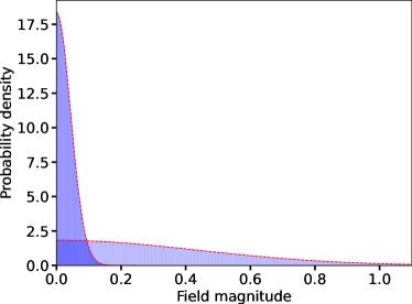
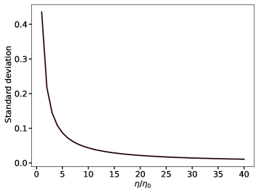
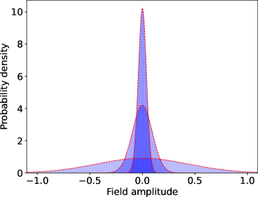
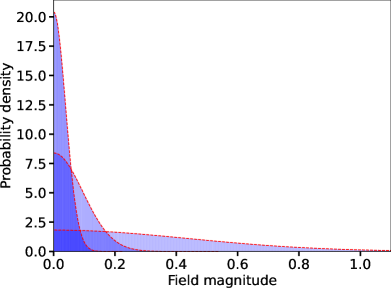
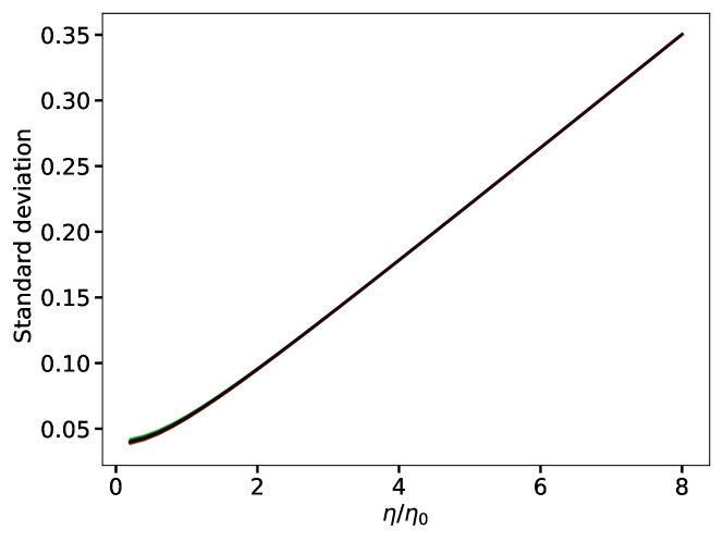
To estimate (62) via random field simulations, we calculate the spatial mean of for each simulation and then average this quantity across all simulations. Since follows the same Gaussian statistics as given by , follows a half-normal distribution (See Fig. 3 and 6 for example). This statistical relation indicates that the spatial average of is given by the standard deviation of , up to a factor of . Using this relation, we can estimate (62) based on the standard deviation of as shown in Fig. 3 and 6, which is taken by averaging the statistics over a large sample of random fields.
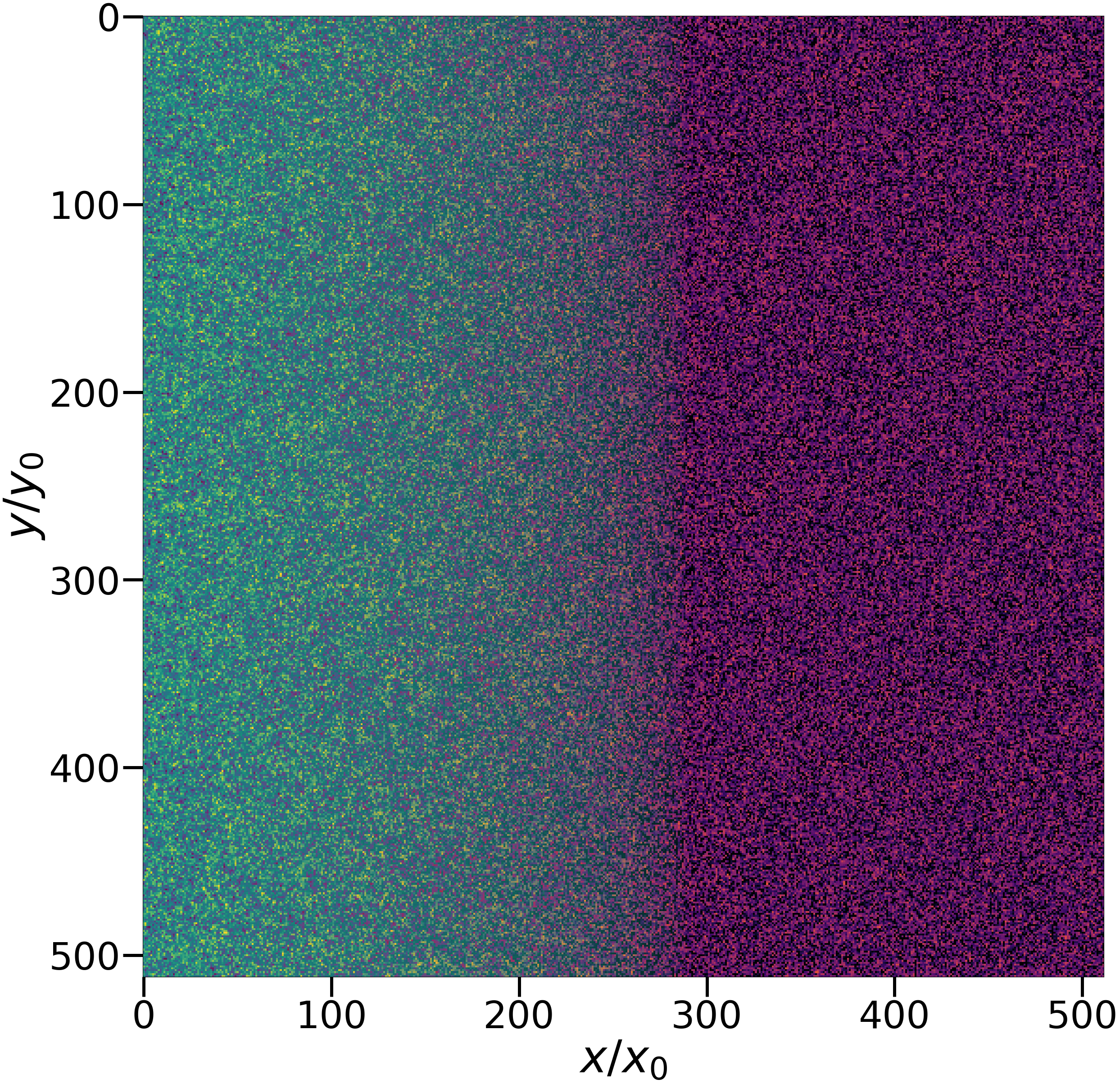
We will investigate two distinct cosmological scenarios: a contracting radiation-dominated universe and an expanding de Sitter spacetime. The former presents a straightforward example to demonstrate the breakdown of the semiclassical framework due to the amplification of quantum fluctuations999 Although our analysis focused on a radiation-dominated universe, it extends generally to any spacetime dynamics that significantly amplify quantum fluctuations, leading inevitably to the same conclusion..
Consider a contracting radiation-dominated universe where with , and set . The mode is given by
| (63) |
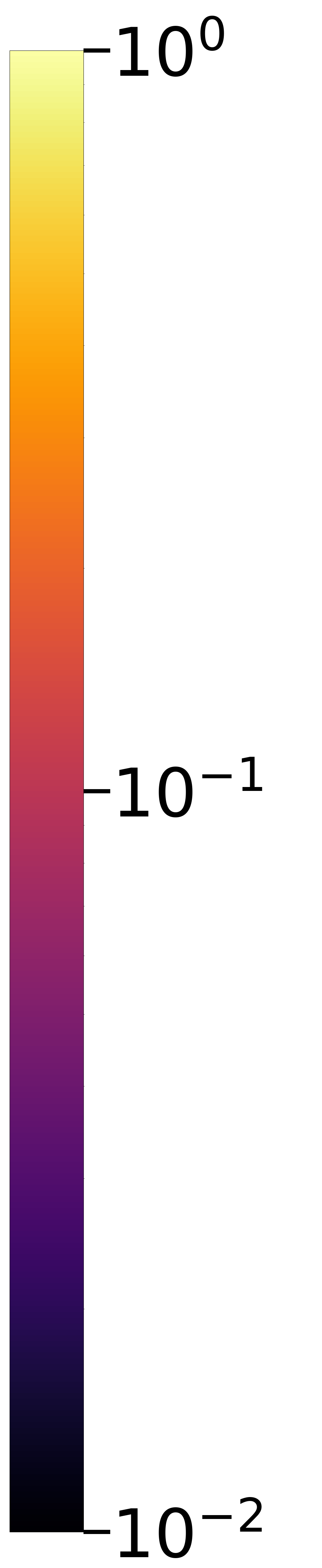
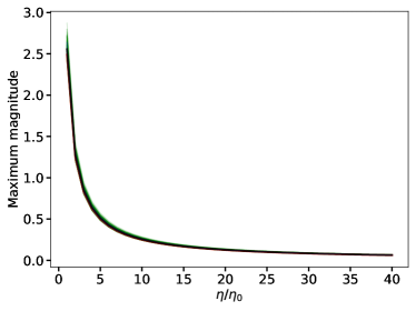
resulting in . This scaling relation () indicates a consistent spatially correlated structure across all , as shown in Fig. 2. In our simulation, we adopted a simple set of parameters101010The specific values are chosen for convenience only. Our analysis can be generalized to any particular choice of , , or . The key point is the relationship between , , and , which dictates the time scale when large-scale structures of relevant length scale emerge, or when the effective framework breaks down. by letting and .
Based on the above parameters, we will test the reliability of the semiclassical approximation using (5) and (6). As a proof concept, we compare with the Hubble parameter , seleected as the classical observable for (6). In a radiation-dominated universe, we expect (6) to hold consistently over time because scales with , which matches the scaling of . This means that (6) remains constant throughout the entire conformal time.
While (6) remains valid, (5) does not hold consistently. As shown in Fig. 2 and 3, the contraction of the radiation-dominated universe significantly amplifies the magnitude of quantum fluctuations. This amplification can become so intense at late times that it drives a significant probability density current to leave the semiclassical domain with boundaries marked by . This is clear in the flattening of the probability density distribution, as shown in Fig. 3.
Additionally, Fig. 2 reveals that the quantum field at is populated with extreme signals everywhere, highlighted as the brightest spots representing . When the system evolves beyond , the semiclassical framework is expected to break down, as will will no longer satisfy the criterion (5), where . The breakdown is even clearer in Fig. 3, where the spatially averaged standard deviation of diverges as .
Consequently, the simulation at should not be considered as an accurate description, but rather as giving the timing when the semiclassical effective framework breaks down.
Note that it is impossible to restore the condition at any later time by restricting ourself to a smaller neighborhood . In fact, this only leads to more severe unitarity loss because a larger proportion of the probability will be excluded from the contraction of the neighborhood, hence further invalidating the existing framework. Given that the standard deviation diverges as in Fig. 3 , we expect the following chain of inequalities upon contracting the neighborhood for :
| (64) |
Ultimately, at some late time , the only possible neighborhood is a set of measure zero with a zero norm.
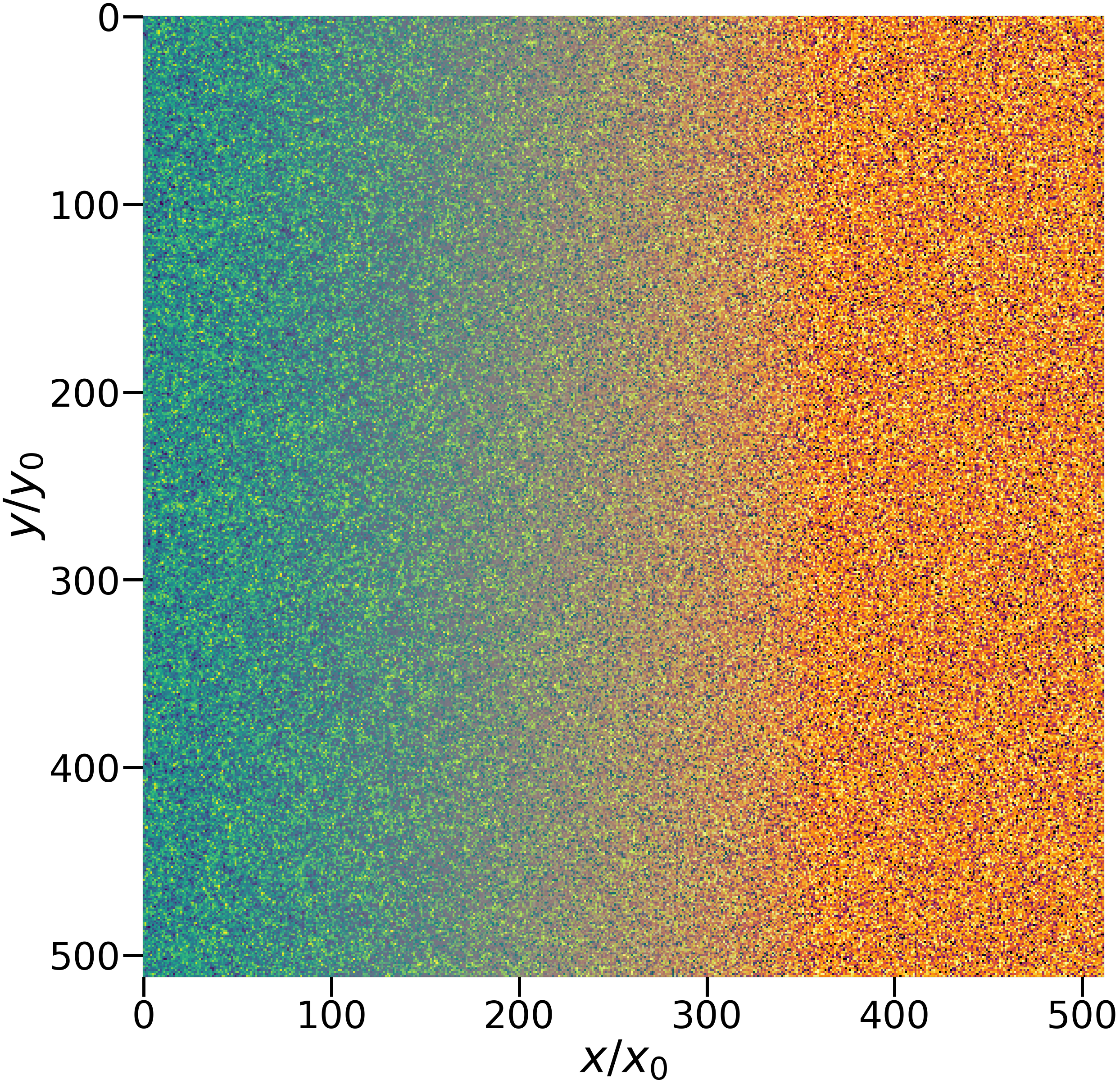
In contrast to the collapsing radiation-dominated universe, the de Sitter spacetime requires a careful selection of initial data. The de Sitter spacetime is characterized by a scale factor for and is the time-independent Hubble parameter, set to for convenient conceptual illustrations. The modes in de Sitter space-time are given by the Hankel functions
| (65) |
where . Adopting the Bunch-Davies vacuum where and [42, 43], the variance becomes . For a minimally coupled massless scalar field (), the Hankel function simplifies:
| (66) |
The explicit form indicates a transition in from to as evolves from to . This suggests the formation of large, spatially correlated structures, which is verified in Fig. LABEL:fig:random_fields_desitter illustrating that their formation effectively begins after (second panel from the left).
Again we consider the criterion (6) where the Hubble parameter is chosen as the classical observable, such that the criterion (6) is given by , for as an example.
In strong contrast to a collapsing radiation-dominated universe, the expansion of the de Sitter universe suppresses the magnitude of quantum fluctuations. This suppression is clearly visible in Fig. LABEL:fig:random_fields_desitter, and further demonstrated by the decrease in standard deviation over time as shown in Fig. 6, alongside the narrowing of the probability distribution in Fig. 5 that indicates a low probability to excite fluctuations of the order of the short distance cut-off scale.
It follows from Fig. 6 that the condition can be consistently fulfilled for all as . However, the problem in de Sitter spacetimes will not arise at the late times, when fluctuations show greater variance in their magnitude as seen in Fig. 6. In other words, fluctuations were more violent in the past. Physically, this implies that while the field configurations are highly reliable at arbitrary late times, it is not sensible to rewind them arbitrarily far back into the past while relying on the semi-classical framework. This underlines the inconsistency of utilizing arbitrary initial data from the distant past, since such data fulfills neither (5), nor (6). Therefore, only initial data after a specific time scale that respects the semiclassical assumption for a given length scale should be selected. Once equipped with valid initial conditions, the subsequent time evolution in de Sitter spacetime can be modeled under the effective semiclassical framework with excellent accuracy into the future.
VI Conclusion
In this article we proposed a diagnostic framework to analyze the domain of validity of effective field theories in semi-classical spacetimes. The framework is based on local geometric requirements in configuration field space that address the effective short-distance incompleteness, as well as stability concerns related to the mean values of observables, which, in turn, restrict the semi-classical domain. This translates to boundaries in configuration field space associated with quantum fluctuations merely shifting the classical background configuration on scales considerably larger than the effective short-distance cut-off, or to boundaries associated with quantum fluctuations triggering sizeable backreactions on smaller scales. In general, probability fluxes penetrating these boundaries lead to spacetime regions populated with quantum fluctuations that are outside the spectrum of fluctuations governed by the effective field theory. Therefore, dynamical aspects of the effective description are given by a contractive evolution (semi-) group, rather than a unitary representation of time translations, in order to account for the probability that is leaking into regions beyond the boundaries in field configuration space. The boundaries depend on the set of observables considered by the observers. Relative to this set the boundaries guarantee the consistency of the effective description, cf (5), and the validity of the semiclassical approximation, cf (6). In fact, (6) measures the magnitude of backreactions which is indicative for the background stability.
In order to quantize the effective field theory, we showed that the basic observables, in our case the configuration and its canonical momentum field, enjoy self-adjoint extensions on a specific Hilbert space. At the kinematic level, the canonical momentum field operator admits infinitely many self-adjoint extensions. Via the usual functional calculus, the analysis extends to the Hamilton operator, again at the kinematic level. However, at the dynamic level, in general, the solution space of the functional Schrödinger equation has no nontrivial intersection with the domains on which the Hamiltonian admits self-adjoint extensions. Important exceptions are static spacetimes. Therefore, provided that the theory is free of ghosts, the evolution must be contractive and the loss of unitarity, usually a sacrosanct requirement for a consistent (but also fundamental) probabilistic framework, has a well-understood reason: The existence of boundaries in field configuration space through which probability can be leaked.
Of course, the loss of unitarity is vital for the existence of a more fundamental description. There are spacetimes that when populated with quantum fluctuations leave the semiclassical approximation intact because potentially harmful field excitations are too rare to impact the large-scale geometry. Intuitively these can be imagined as almost static or mildly dynamic spacetimes. Contrary to these there are spacetimes that support the excitation of free quantum fluctuations that trigger background instabilities and invalidate the semiclassical approximation at the global level.
In order to demonstrate the framework developed in this work, we complement our formal analysis by numerical experiments. As a proof of concept, with the aid of our numerical experiments, we identify regions in cosmological spacetimes, where freely evolving quantum fluctuations violate unitarity to an extent that the semiclassical approximation is locally invalidated. As a concrete example, we consider a collapsing universe filled with radiation. This spacetime geometry borders on a future singularity. As can be expected, there is a substantial probability flux in its vicinity penetrating the configuration field boundaries, thereby exciting fluctuations that destabilize the background, leading to a breakdown of the semiclassical approximation (Fig.3). In contrast, and as another example, we consider quantum fluctuations populating de Sitter spacetime: In this case the semiclassical approximation holds towards the future (given appropriate initial conditions), but ceases to hold in the past. This indicates that semiclassicality further restricts acceptable initial conditions by limiting the time domain where initial quantization is performed. This is crucial because, even if regular initial conditions are chosen by hand, the semiclassical approximation can immediately break down once the system evolves outside the allowed time domain.
Acknowledgements.
KHC thanks James Creswell for his expertise and discussions on topics related to Gaussian random fields. The authors thank Maximilian Koegler for the initial collaboration on a related topic. MS has been supported by the Italian Ministry of Education and Scientific Research (MIUR) under the grant PRIN MIUR 2017-MB8AEZ. KHC has been financially supported by the Excellence Cluster ORIGINS.Appendix A Notation and Conventions
Throughout this article use the following convention and conventions: smeared operators are defined by , where denotes a spatial submanifold, the metric determinant of , and are smooth smearing functions of compactly supported on . Integral signs are mostly expressed by for spatial integral, and for the momentum integral within some momentum space. Concerning the metric, we will use mostly plus signature and we will work in natural units for the theoretical as well as the simulation part, if not stated differently.
Appendix B Normality Test
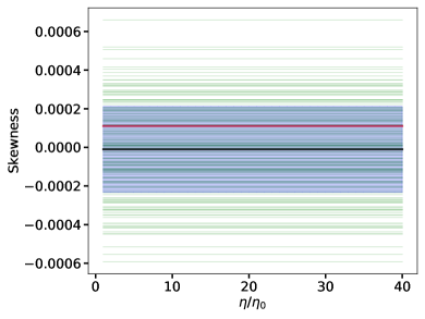
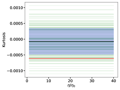
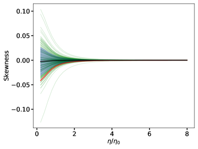
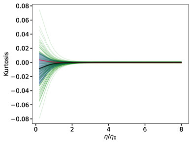
In this section, we examine the normality of the Gaussian random fields simulated in de Sitter spacetime and the radiation-dominated universe. Our statistical analysis focuses on the higher moments of the random fields, specifically the kurtosis and skewness.
Fig. 7 reveals a strong contrast between the previously considered scenarios: in the radiation-dominated universe, the probability density distribution of the Gaussian random field shows negligible higher moments that remain constant under time-evolution, indicating minimal deviation from normality. Instead, in the de Sitter spacetime, the higher moments grow in time as large-scale structures begin to form. We can see from Fig. 7 that the development of large-scale structure introduces a non-trivial skewness and kurtosis in the probability distributions (Green curve).
The underlying cause of this phenomenon appears to lie the highly correlated nature of our simulation data, combined with the limitations of data size. In de Sitter space, the spatial correlation is characterized by a scaling in the power spectrum which implies that a neighborhood region is likely to contain signals of similar amplitude. This effect is particularly significant in de Sitter geometry, where the correlation length is comparable to the full simulation scale (See Fig. LABEL:fig:random_fields_desitter).
Although higher moments develop in each individual simulation, the statistical average of skewness across all simulations is approximately zero, with a minor negative averaged excess of kurtosis (black curve in 7). This is important because it shows that there are no preferred higher moments across all simulations. As more data is sampled, this diminishing effect is expected to suppress higher moments further.
References
- Vilenkin [1989] A. Vilenkin, Phys. Rev. D 39, 1116 (1989).
- Kuo and Ford [1993] C.-I. Kuo and L. H. Ford, Phys. Rev. D 47, 4510 (1993), arXiv:gr-qc/9304008 .
- Matsui and Watamura [2020] H. Matsui and N. Watamura, Physical Review D 101, 025014 (2020).
- Massar and Parentani [1999] S. Massar and R. Parentani, Physical Review D 59, 123519 (1999).
- Anderson et al. [2003] P. R. Anderson, C. Molina-Paris, and E. Mottola, Physical Review D 67, 024026 (2003).
- Reed and Simon [1975] M. Reed and B. Simon, Methods of modern mathematical physics, Vol. II (Academic Press, New York, 1975).
- Burgess et al. [2009] C. P. Burgess, H. M. Lee, and M. Trott, JHEP 09, 103, arXiv:0902.4465 [hep-ph] .
- Eboli et al. [1989] O. J. P. Eboli, S.-Y. Pi, and M. Samiullah, Annals Phys. 193, 102 (1989).
- Hatfield [2018] B. Hatfield, Quantum field theory of point particles and strings (CRC Press, 2018).
- Halliwell [1991] J. J. Halliwell, Phys. Rev. D 43, 2590 (1991).
- Long and Shore [1998] D. V. Long and G. M. Shore, Nucl. Phys. B 530, 247 (1998), arXiv:hep-th/9605004 .
- Traschen and Brandenberger [1990] J. H. Traschen and R. H. Brandenberger, Phys. Rev. D 42, 2491 (1990).
- Guth and Pi [1985] A. H. Guth and S.-Y. Pi, Physical Review D 32, 1899 (1985).
- Boyanovsky et al. [1994] D. Boyanovsky, H. J. de Vega, and R. Holman, Phys. Rev. D 49, 2769 (1994).
- Floreanini et al. [1987] R. Floreanini, C. T. Hill, and R. Jackiw, Annals Phys. 175, 345 (1987).
- Guven et al. [1989] J. Guven, B. Lieberman, and C. T. Hill, Phys. Rev. D 39, 438 (1989).
- Hofmann and Schneider [2015] S. Hofmann and M. Schneider, Phys. Rev. D 91, 125028 (2015), arXiv:1504.05580 [hep-th] .
- Hofmann and Schneider [2017] S. Hofmann and M. Schneider, Phys. Rev. D 95, 065033 (2017), arXiv:1611.07981 [hep-th] .
- Eglseer et al. [2021] L. Eglseer, S. Hofmann, and M. Schneider, Phys. Rev. D 104, 105010 (2021), arXiv:1710.07645 [hep-th] .
- Hofmann et al. [2019] S. Hofmann, M. Schneider, and M. Urban, Phys. Rev. D 99, 065012 (2019), arXiv:1901.04492 [hep-th] .
- Callan and Wilczek [1994] C. G. Callan, Jr. and F. Wilczek, Phys. Lett. B 333, 55 (1994), arXiv:hep-th/9401072 .
- Berges et al. [2018] J. Berges, S. Floerchinger, and R. Venugopalan, JHEP 04, 145, arXiv:1712.09362 [hep-th] .
- Corichi et al. [2002] A. Corichi, J. Cortez, and H. Quevedo, Phys. Rev. D 66, 085025 (2002), arXiv:gr-qc/0207088 .
- Torre and Varadarajan [1998] C. G. Torre and M. Varadarajan, Physical Review D 58, 064007 (1998).
- Alonso et al. [2024a] J. L. Alonso, C. Bouthelier-Madre, J. Clemente-Gallardo, and D. Martínez-Crespo, Class. Quant. Grav. 41, 105004 (2024a), arXiv:2307.00922 [gr-qc] .
- Alonso et al. [2024b] J. L. Alonso, C. Bouthelier-Madre, J. Clemente-Gallardo, and D. Martínez-Crespo, J. Geom. Phys. 203, 105264 (2024b), arXiv:2306.14844 [math-ph] .
- Alonso et al. [2024c] J. L. Alonso, C. Bouthelier-Madre, J. Clemente-Gallardo, and D. Martínez-Crespo, J. Geom. Phys. 203, 105265 (2024c), arXiv:2402.07953 [math-ph] .
- Geroch [1970] R. Geroch, Journal of Mathematical Physics 11, 437 (1970).
- Fredenhagen and Rejzner [2015] K. Fredenhagen and K. Rejzner, Advances in algebraic quantum field theory , 31 (2015).
- Reed and Simon [1980] M. Reed and B. Simon, Methods of modern mathematical physics. vol. 1. Functional analysis (Academic, 1980).
- Reed and Simon [1979] M. Reed and B. Simon, Methods of mathematical physics III: Scattering Theory (Academic Press, New York, 1979).
- DeWitt [2003] B. S. DeWitt, The global approach to quantum field theory, Vol. 114 (Oxford University Press, USA, 2003).
- Schneider [2018] M. M. Schneider, Black holes are quantum complete, Ph.D. thesis, Munich U. (2018).
- Ashtekar and Magnon [1975] A. Ashtekar and A. Magnon, Proc. Roy. Soc. Lond. A 346, 375 (1975).
- Parker and Toms [2009] L. E. Parker and D. Toms, Quantum Field Theory in Curved Spacetime: Quantized Field and Gravity, Cambridge Monographs on Mathematical Physics (Cambridge University Press, 2009).
- Mukhanov and Winitzki [2007] V. Mukhanov and S. Winitzki, Introduction to quantum effects in gravity (Cambridge University Press, 2007).
- Pi [1990] S. Pi, in Field theory and particle physics (1990).
- Hristopulos [2020] D. T. Hristopulos, Random fields for spatial data modeling (Springer, 2020).
- Bertschinger [2001] E. Bertschinger, The Astrophysical Journal Supplement Series 137, 1–20 (2001).
- Mukhanov et al. [1992] V. F. Mukhanov, H. A. Feldman, and R. H. Brandenberger, Phys. Rept. 215, 203 (1992).
- Mukhanov [2005] V. Mukhanov, Physical Foundations of Cosmology (Cambridge University Press, Oxford, 2005).
- Bunch and Davies [1978] T. S. Bunch and P. C. Davies, Proceedings of the Royal Society of London. A. Mathematical and Physical Sciences 360, 117 (1978).
- Birrell and Davies [1984] N. D. Birrell and P. C. W. Davies, Quantum Fields in Curved Space, Cambridge Monographs on Mathematical Physics (Cambridge Univ. Press, Cambridge, UK, 1984).