Nature cannot be described by any causal theory with a finite number of measurements

Abstract

We show, for any $n\geq 2$, that there exists quantum correlations obtained from performing $n$ dichotomic quantum measurements in a bipartite Bell scenario, which cannot be reproduced by $n-1$ measurements in any causal theory. That is, it requires any no-signaling theory an unbounded number of measurements to reproduce the predictions of quantum theory. We prove our results by showing that there exists Bell inequalities that have to be obeyed by any no-signaling theory involving only $n-1$ measurements and show explicitly how these can be violated in quantum theory. Finally, we discuss the relation of our work to previous works ruling out alternatives to quantum theory with some kind of bounded degree of freedom and consider the experimental verifiability of our results.

Introduction.—Quantum theory is the most successful and accurately tested description of nature that exists in physics Hanneke et al. (2008); Sailer et al. (2022). In its essence, quantum theory is a set of mathematical rules leading to observable predictions. However, we are still lacking the concise physical principles obeyed by nature that lead to the corresponding mathematical framework Wheeler (1989); Chiribella and Spekkens (2016). Even more crucially, to our current knowledge, there is still room for theories beyond quantum theory that might describe nature more accurately, which are in agreement with well-motivated physical principles, such as causality (by virtue of the no-signaling principle) Popescu and Rohrlich (1992); Janotta (2012). It is therefore critical to study alternative theories that are close to quantum theory and to understand whether they can be ruled out Navascués et al. (2015); Pawłowski et al. (2009); Fritz et al. (2013); Brassard et al. (2006); Renou et al. (2021); Coiteux-Roy et al. (2021); Kleinmann and Cabello (2016); Renou et al. (2021).
The most powerful tool available to rule out alternative descriptions of nature to quantum theory is Bell’s theorem Bell (1964) and Bell’s inequalities. Initially devised to rule out the possibility of theories based on the premise of local hidden variables Einstein et al. (1935), which has been demonstrated in many groundbreaking experiments Rosenfeld et al. (2017); Giustina et al. (2015); Hensen et al. (2015); Shalm et al. (2015), the success of Bell’s theorem goes way beyond its initial use Brunner et al. (2014); Tavakoli et al. (2022). In particular, Bell’s theorem can be used to self-test quantum systems Šupić and Bowles (2020), proof the security of cryptography protocols with minimal assumptions Ekert (1991); Acín et al. (2007), and for witnessing the generation of genuine randomness Colbeck (2009); Pironio et al. (2010); Colbeck and Kent (2011).
On a more fundamental level, the violation of a Bell inequality certifies the presence of entangled systems Horodecki et al. (2009); Moroder et al. (2013) (i.e., systems that cannot be prepared by local operations only) and incompatible measurements Gühne et al. (2023); Heinosaari et al. (2016); Chen et al. (2021); Quintino et al. (2019); Fine (1982); Wolf et al. (2009); Cavalcanti and Skrzypczyk (2016) (i.e., specific observable quantities that cannot be measured jointly via a single measurement). Crucially, entanglement and incompatibility are necessary requirements for the violation of a Bell inequality not only in quantum theory but in much more general theories leading to probabilistic observations, so called general probabilistic theories Acín et al. (2010); Plávala (2023); Banik (2015); Plávala (2016), which quantum theory is a special case of.
Judiciously chosen Bell scenarios have been used in the past to rule of causal theories of nature with only: a finite number of measurement outcomes Kleinmann and Cabello (2016), a finite number of entangled parties Collins et al. (2002); Seevinck and Svetlichny (2002), and sources of correlations of finite degree Coiteux-Roy et al. (2021). Hence, Bell’s theorem can be used to proof that nature does not allow for a finite bound on many external parameters (i.e., parameters that are not part of the mathematical theory but more of the Bell experiment itself).

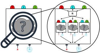
Figure 1: Graphical representation of our main question. Measurement devices are treated as black-boxes, without even assuming the physical theory they are governed by. Just on the basis of the input-output statics, we rule out that the inner workings of the measurement device include a randomized process $\mathrm{R}$ and measurement devices with fewer inputs to simulate the considered device. While it is here only shown for $3$ measurements that are simulated by devices of effectively $2$ measurements, we rule out that this is generally possibility for all causal theories and any finite number of measurements $n\geq 2$.

However, the question regarding the possible boundlessness of the number of measurements needed to describe nature remains unanswered. Surprisingly, recent progress Kleinmann et al. (2017); Quintino et al. (2019) has been only able to show that nature cannot be described with just $2$ measurements (see also Figure 1), leaving a general answer to the question: Can nature possibly be described by a (maybe very exotic) causal theory that only requires a finite number of measurements? widely open.
In this work, we answer exactly this question in the negative, that means we show that nature cannot be described by any causal theory that involves only a finite number of measurements. In particular, we show the existence of quantum correlations obtained from performing $n$ different dichotomic measurement on an bipartite entangled quantum state that cannot be reproduced by any theory of nature (classical, quantum, and beyond), which is compatible with causality (i.e., it does not allow for super luminal signalling) involving only $n-1$ measurements for every finite $n$. Hence, every possible way to come up with a, maybe very exotic, causal theory of nature in which there is an (arbitrarily large but finite) upper limit on the number of different measurement settings, can be falsified. We want to emphasize at this point that the terms causal theory or causality, which are overloaded with various non-equivalent definitions in quantum information theory, are used synonymous to no-signaling theory throughout this manuscript.
To prove our result, we consider the theory of measurement incompatibility, whose extension to recently studied incompatibility structures Kunjwal et al. (2014); Heinosaari et al. (2008); Liang et al. (2011); Quintino et al. (2019); Tendick et al. (2023) is crucial to formally define what it means for $n$ measurements to be genuinely incompatible, i.e., not reducible to $n-1$ measurements. We then connect genuine incompatibility to the family of $M_{nn22}$ inequalities Brunner et al. (2006), to show that a violation of these inequalities implies the existence of genuinely $n$ measurements in a theory independent way, i.e., without assuming the formalism of a specific theory but only relying on causality by virtue of the no-signaling principle. We then show that any of the $M_{nn22}$ can be violated by quantum theory with a quantum state of local dimension $n$. Finally we discuss possible experimental implementations of our findings.
Incompatible measurements in nature.—Let us start by reviewing the notions of incompatibility and how to test device and theory independently that there exist observable quantities that cannot be measured jointly. In quantum theory, measurements are described by positive semidefinite operators $A_{a|x}\geq 0$ acting on a Hilbert space $\mathcal{H}\cong\mathds{C}^{d}$ of dimension $d$, such that the completeness relation $\sum_{a}A_{a|x}=\mathds{1}$, (where $\mathds{1}$ is the identity operator), is fulfilled. Here, $x$ denotes the label of a specific measurement and $a$ the label of the corresponding outcome to that measurement. We say a set of measurements (also known as assemblage) $\mathcal{A}=\{\{A_{a|x}\}_{a}\}_{x}$ is jointly measurable if it can be simulated by performing a single measurement $\{G_{\lambda}\}_{\lambda}$ (the so-called parent positive operator valued measure (POVM)) and some classical post-processing via the conditional probabilities $p(a|x,\lambda)$ such that

$$A_{a|x}=\sum_{\lambda}p(a|x\lambda)G_{\lambda},$$ (1)

holds. An assemblage that is not jointly measurable is called incompatible. Note that joint measurability can conceptually be seen as the generalization of commutativity of projective measurements to general quantum measurements Heinosaari et al. (2016); Gühne et al. (2023).
To demonstrate incompatibility of measurements without needing a full characterization of the measurement device, or the physical theory it is governed by, one needs to rely on the device-independent paradigm and the violation of Bell inequalities. Let us consider a bipartite Bell experiment in which two distant parties, Alice and Bob, perform one out of $n$ measurements in each round of the experiment labeled by $x$ and $y$, respectively. In each round, Alice obtains one out of two outcomes $a$, similarly Bob obtains outcome $b$. Treating their devices as black-boxes, all information about the experiment that is accessible to Alice and Bob are the input-output statistics, also called behaviour or correlations, $\mathbf{P}=\{p(ab|xy)\}$. Just on the basis of the obtained behaviour $\mathbf{P}$ we want to prove that the considered black-box devices involve indeed incompatible measurements and hence cannot be treated as a single measurement.
In the case of $n=2$ measurements we can do so by looking at the Clauser-Horne-Shimony-Holt (CHSH) inequality Clauser et al. (1969) given by (in the notation of Collins-Gisin Collins and Gisin (2004))

$$p(00|11)+p(00|12) +p(00|21)-p(00|22)$$

$$-p_{A}(0|1)-p_{B}(0|1)\leq 0.$$ (2)

By definition of being a Bell inequality, the CHSH inequality has to be obeyed by all local (also known as classical) theories, i.e., by all theories where the correlations $\mathbf{P}$ could be explained via pre-shared randomness. However, it is well-known that quantum correlations obtained from performing quantum measurements on a shared bipartite quantum state $\rho$ such that $p(ab|xy)=\mathrm{Tr}[(A_{a|x}\otimes B_{b|y})\rho]$ can violate the CHSH inequality, provided judiciously chosen incompatible measurements $\mathcal{A},\mathcal{B}$ are performed on an entangled state $\rho$. That is, the CHSH inequality certifies in a device-independent way the existence of entanglement and for us more importantly, that Alice and Bob each employed incompatible measurements. While incompatibility is necessary for the violation of a Bell inequality, it is known that is generally not sufficient Bene and Vértesi (2018); Hirsch et al. (2018) and it is an open question which incompatibility structures can be certified device-independently.
In their seminal work, Wolf et al. Wolf et al. (2009) prove that any pair of incompatible dichotomic measurements can be used to violate the CHSH inequality if the measurements of the other party and the quantum state $\rho$ are optimized accordingly. Moreover, the authors in Wolf et al. (2009) prove that the violation of a general Bell inequality not only implies the incompatibility of measurements in quantum theory, but in any theory that obeys the no-signaling principle. The no-signaling principle states that the measurement devices of Alice and Bob cannot be used for superluminal signaling, which can be seen as a basic definition for a physical theory to obey causality. More formally, the correlations $\mathbf{P}$ obey the no-signaling principle Popescu and Rohrlich (1992); Janotta (2012), if their marginal distributions $p_{A}(a|x)$ and $p_{B}(b|y)$ are well-defined and independent of the input of the other party, i.e., $p_{A}(a|x)=p_{A}(a|xy)=\sum_{b}p(ab\lvert xy)$ for all $a,x,$ and similarly for Bob’s marginal. However, the general question of whether there always exist $n$ measurements, for any $n\geq 2$, that cannot be reproduced by at most $n-1$ measurements in any causal theory remains still open.
Boundlessly many genuine incompatible measurements in nature.—Here, we answer this question affirmatively. To hat end, we first have to define properly what it means to have genuinely $n$ measurements. While ordinary incompatibility according to Eq. (1) only guarantees that the assemblage $\mathcal{A}$ cannot be reduced to a single measurement, it does not guarantee that $n$ measurements cannot be reduced to fewer measurements in general. Using the notion of recently studied incompatibility structures, the authors in Quintino et al. (2019) define an assemblage to contain (at least) genuinely $n$ measurements if it cannot be implemented by probabilistically employing assemblages that contain at most genuinely $n-1$ measurements. That is, if the assemblage $\mathcal{A}$ cannot be decomposed such that

$$A_{a|x}=\sum_{(s,t\neq s)\in\mathcal{T}}p_{(s,t)}F_{a|x}^{(s,t)},$$ (3)

where $\mathcal{F}^{(s,t)}\in\mathrm{JM}^{(s,t)}$ are assemblages, employed with probability $p_{(s,t)}$, in which the pair $(s,t\neq s)$ is jointly measurable, which makes each $\mathcal{F}^{(s,t)}$ contain at most genuinely $n-1$ measurements (as the pair $(s,t\neq s)$ is one effective measurement) and the set $\mathcal{T}$ contains all tuples $(s,t\neq s)$ constructed from the integers $\{1,\cdots,n\}$.
The key observation of Quintino et al. (2019) is using the fact that an incompatibility structure like in Eq. (3) results in restrictions on the observable behaviour $\mathbf{P}$ that then can be used in Bell scenarios to certify that certain measurements do not obey a given incompatibility structure. More precisely, assuming that Bob’s measurements obey an incompatibility structure according to Eq. (3) leads to a decomposition of the behaviour $\mathbf{P}$ of the form

$$p(ab|xy)=\sum_{(s,t\neq s)\in\mathcal{T}}p_{(s,t)}p^{(s,t)}(ab|xy),$$ (4)

where $p^{(s,t)}(ab|xy)$ describes a behaviour $\mathbf{P}^{(s,t)}$ that is local once it is restricted to only the measurements $(s,t)$ on Bob’s side. Now, crucially, disproving that a decomposition according to Eq. (4) exists while only assuming the no-signaling principle, constitutes a device and theory independent proof of having access to genuinely $n$ measurements.
The numerical analysis for the case $n=3$ in Quintino et al. (2019) reveals that while it is easy to use many well known inequalities like the $3$-CHSH game Bowles et al. (2018), the elegant Gisin (2007), or the chained Bell inequality Braunstein and Caves (1990) for the certification of genuinely $3$ measurements assuming quantum theory, it is more difficult to rule out the possibility of a simulation by only $2$ measurements in general no-signaling theories. Essentially, there exists only one relevant Bell inequality, the $M_{3322}$ inequality for this task (see also Kleinmann et al. (2017)), which was already and independently been considered in Brunner et al. (2004). However, the $M_{3322}$ inequality only allows for a relatively small violation within quantum theory and employing numerical methods can only provide insights for small number of measurements $n$. Hence, despite providing the best current progress, the methods in Bowles et al. (2018) are of limited use for answering our main question.
We show in the following that a detailed analytical analysis of why the $M_{3322}$ certifies genuinely $3$ measurements in any causal theory leads to the key observation that enables us to prove our main result. More precisely, it enables us for every finite integer $n\geq 2$, to propose a Bell experiment, including $n$ dichotomic quantum measurements, that cannot be reproduced by any causal (i.e., no-signaling) theory using only $n-1$ measurements. Let us denote the set of no-signaling correlations of at most genuinely $n$ measurements according to Eq. (4) by $\mathrm{GNS}_{n}$.

Main result.

For every $n\geq 2$ there exist quantum correlations $\mathbf{Q}\in\mathrm{GNS}_{n}$ that cannot be reproduced by any no-signaling correlations with at most genuinely $n-1$ measurements, i.e., $\mathbf{Q}\notin\mathrm{GNS}_{n-1}$.

Proof.

Let us start by analytically analyzing why the $M_{3322}$ inequality cannot be violated by distributions $\mathbf{P}\in\mathrm{GNS}_{2}$. To make the proof as vivid as possible, we will work with the Collins-Gisin table notation of behaviours $\mathbf{P}$ and Bell inequalities to understand the structure of the considered inequalities better. In particular, any normalized no-signaling behaviour $\mathbf{P}$ of two-outcome measurements in uniquely characterized by a table (shown here for two settings)

$$\begin{array}[]{c||c c}&P(A_{1})&P(A_{2})\\ \hline\cr\hline\cr P(B_{1})&P(A_{1}B_{1})&P(A_{2}B_{1})\\ P(B_{2})&P(A_{1}B_{2})&P(A_{2}B_{2})\\ \end{array},$$ (8)

where $P(A_{1})\coloneqq p_{A}(a=0|x=1)$, $P(A_{1}B_{1})\coloneqq p(a=0,b=0\lvert x=1,y=1)$ and similarly for the other terms with a straightforward generalization to more settings. Similarly, we represent Bell inequalities by a table of coefficients corresponding to the probability they are multiplied with. In this notation, the $M_{3322}$ inequality is given by

$$M_{3322}= \begin{array}[]{c||c c c}&-2&\phantom{-}0&\phantom{-}0\\ \hline\cr\hline\cr-2&\phantom{-}1&\phantom{-}1&\phantom{-}1\\ -1&\phantom{-}1&\phantom{-}1&-1\\ \phantom{-}0&\phantom{-}1&-1&\phantom{-}0\\ \end{array}\leq 0.$$ (13)

Using the fact that for any no-signaling distribution the marginal distributions upper bound their involved correlations, i.e., $P(A_{k})\geq P(A_{k}B_{j})$ and $P(B_{k})\geq P(A_{j}B_{k})$, we can deduce consequences on the incompatibility structures that follow from a violation of $M_{3322}$. Namely, it follows that $M_{3322}>0$ implies a simultaneous violation of the inequalities

$$M_{3322}^{(1,2)}= \begin{array}[]{c||c c c}&-1&\phantom{-}0&\phantom{-}0\\ \hline\cr\hline\cr-1&\phantom{-}1&\phantom{-}0&\phantom{-}1\\ \phantom{-}0&\phantom{-}1&\phantom{-}0&-1\\ \phantom{-}0&\phantom{-}0&\phantom{-}0&\phantom{-}0\\ \end{array}\leq 0,$$ (18)

$$M_{3322}^{(1,3)}= \begin{array}[]{c||c c c}&-1&\phantom{-}0&\phantom{-}0\\ \hline\cr\hline\cr-1&\phantom{-}1&\phantom{-}1&\phantom{-}0\\ \phantom{-}0&\phantom{-}0&\phantom{-}0&\phantom{-}0\\ \phantom{-}0&\phantom{-}1&-1&\phantom{-}0\\ \end{array}\leq 0,$$ (23)

and

$$M_{3322}^{(2,3)}= \begin{array}[]{c||c c c}&-1&\phantom{-}0&\phantom{-}0\\ \hline\cr\hline\cr\phantom{-}0&\phantom{-}0&\phantom{-}0&\phantom{-}0\\ -1&\phantom{-}1&\phantom{-}1&\phantom{-}0\\ \phantom{-}0&\phantom{-}1&-1&\phantom{-}0\\ \end{array}\leq 0.$$ (28)

To see this, we only have to realize that simultaneously erasing positive contributions like $P(A_{k}B_{j})$ and negative contributions $P(A_{k})$ makes it easier to violate the inequality, as the total contribution of these terms would be negative. A similar reasoning follows for erasing terms $P(A_{k}B_{j})$ that contribute with a negative sign. Now, this means every pair of two measurements of Bob has to lead to nonlocal correlations, as each of the above versions of the $M_{3322}^{(s,t)}$ is equivalent to the CHSH inequality for the pair $(s,t)$. Hence, every pair of Bob’s measurements has to be incompatible. By contra position, if one the pairs $(s,t)$ is compatible, it holds $M_{3322}^{(s,t)}\leq 0$. That means, the upper bound $M_{3322}\leq 0$ holds for all no-signaling distributions $\mathbf{P}$ in which some pair $(s,t)$ leads to local correlations. Now, by convexity of the decomposition in Eq. (4) and the fact that $M_{3322}$ is a linear Bell inequality, the same also holds for any behaviour $\mathbf{P}\in\mathrm{GNS}_{2}$.
For general $n\geq 2$, we consider the $M_{nn22}$ inequalities Brunner et al. (2006), (of which $M_{3322}$ is simple the $n=3$ case) derived from slightly varying the family of $I_{nn22}$ inequalities Collins and Gisin (2004). More formally, it holds $M_{nn22}\coloneqq I_{nn22}-(n-2)p_{A}(a=0|x=1)$ or

$$M_{nn22}=\begin{array}[]{c|| cccccc}\mbox{}&-(n-1)&\phantom{-}0&\phantom{-}0&\cdots&\phantom{-}0&\phantom{-}0\\ \hline\cr\hline\cr-(n-1)&\phantom{-}1&\phantom{-}1&\phantom{-}1&\cdots&\phantom{-}1&\phantom{-}1\\ -(n-2)&\phantom{-}1&\phantom{-}1&\phantom{-}1&\cdots&\phantom{-}1&-1\\ -(n-3)&\phantom{-}1&\phantom{-}1&\phantom{-}1&\cdots&-1&\phantom{-}0\\ \phantom{-}\vdots&\phantom{-}\vdots&\mbox{}&\mbox{}&\mbox{}&\mbox{}&\phantom{-}\vdots\\ -1&\phantom{-}1&\phantom{-}1&-1&\cdots&\phantom{-}0&\phantom{-}0\\ \phantom{-}0&\phantom{-}1&-1&\phantom{-}0&\cdots&\phantom{-}0&\phantom{-}0\end{array}\leq 0.$$ (36)

We generalize the above analysis in the Supplemental Material (SM) Sup , i.e., we show that there exist a version of the CHSH inequality for every pair $(s,t)$ of Bob’s measurements that has to be violated if $M_{nn22}$ is violated. Consequently, it holds $M_{nn22}\leq 0$ for all correlations $\mathbf{P}\in\mathrm{GNS}_{n-1}$ originating from at most $n-1$ genuine measurements on Bob’s side according to Eq. (4).
Finally, it is know that all $I_{nn22}$ can be violated via the specific implementation found in Vértesi et al. (2010). It can be checked that the same holds for the $M_{nn22}$ inequalities. In particular, we use a quantum state

$$\lvert\Psi_{\epsilon}\rangle=\sqrt{\dfrac{1-\epsilon^{2}}{n-1}}\sum_{k=1}^{n-1}\lvert kk\rangle+\epsilon\lvert nn\rangle,$$ (37)

of local dimension $n$, parameterized by $\epsilon\in[0,1]$. Using particular projective measurements defined in Vértesi et al. (2010), we obtain a Bell value of

$$M_{nn22}(\mathbf{Q})=\epsilon^{2}(q_{0}^{2}n-(n-1)),$$ (38)

where $\epsilon^{2}=\tfrac{1-q_{0}^{2}}{1+[(n-1)^{2}-1]q_{0}^{2}}$ and $0\leq q_{0}\leq 1$. This gives a violation which is strictly positive (but arbitrarily small for large $n$) whenever $\sqrt{\tfrac{n-1}{n}}<q_{0}<1$. This finishes the proof. ∎

Toward experimental implementations.—As our proof is constructive, i.e., we provide a particular Bell inequality that can be violated by a specific (known) quantum implementation, it raises the question whether our results could experimentally be verified for low number of settings $n$. Indeed, the $M_{3322}$ has experimentally already been violated in Christensen et al. (2015), even with qubit systems. Meaning the first interesting case arises for $n=4$. One challenge that an experimental verification has to face is the relatively low violation achievable according to Eq. (38). We argue here that this is a general feature of the family of $M_{nn22}$ inequalities and not particular to the specific implementation used here. To that end, we note that the maximal possible quantum violation of the $M_{nn22}$ inequality decreases generally for all quantum correlations, according to the third level of the NPA hierarchy Navascués et al. (2007). For instance, while it holds in general quantum theory that $M_{3322}(\mathbf{Q})\leq 0.0324$, already for $n=5$ measurements we only can hope to observe a violation of one order of magnitude less, i.e., $M_{5522}(\mathbf{Q})\leq 0.0040$. In contrast to that, by maximizing Eq. (38) we can reach a value of $M_{3322}(\mathbf{Q})\approx 0.0239$ for $n=3$ measurements and $M_{5522}(\mathbf{Q})\approx 0.0035$ for $n=5$ measurements.
Nevertheless, recent experimental progress in high-dimensional detection loophole-free Bell tests Hu et al. (2022) have been able to generate the quantum state in Eq. (37) for $n=4$ with a fidelity of $99.5\%$ using path entanglement. While different measurements and a different Bell inequality have been considered in Hu et al. (2022), the employed techniques and measurements are close Vértesi et al. (2010) to what is required for a violation of the $M_{4422}$ inequality using four dimensional systems. In conclusion, these recent developments still leave the question of an experimental violation of the $M_{4422}$ and hence an experimental falsification of no-signaling theories using only genuinely $3$ measurements open but within reach of what is accessible with state-of-the-art technologies.
Discussion.—We have proven that, for every finite integer $n\geq 2$, there exist quantum correlations that employ genuinely $n$ measurements in any causal theory of nature. That is, there cannot exist a no-signaling theory in which the predictions of quantum theory are reproduced by using only genuinely $n-1$ or less measurements. Astonishingly, given that the predictions for quantum theory on the particular implementation used in our main result are correct, our result implies that nature cannot be described by a finite number of measurements. Our proof relies on an analytic application of the framework of incompatibility structures to the family of $M_{nn22}$, showing that they constitute a device-independent and theory-independent witness of $n$ genuine measurements. We then argued that a practical verification of our results for low $n$, with particular focus on the case $n=4$ are within experimental reach.
Our works proves that any causal description of nature (including quantum and post-quantum theories) does not only require more than $2$ measurements Quintino et al. (2019) but the number of required measurements is actually unbounded. At the same time, our results provide also an analogue to the findings in Kleinmann and Cabello (2016); Kleinmann et al. (2017), which imply that the predictions of quantum theory cannot be reproduced by a finite number of measurement outcomes. There is an interesting parallel between the latter works and our results, as they require the Hilbert space dimension of the quantum system used for the Bell inequality violation to grow with $n$. While it is unclear whether this phenomenon is a necessity (in particular because $M_{3322}$ can be violated with qubits) it is reasonable to assume that it becomes increasingly harder to distinguish quantum theory from a no-signaling theory restricted to $n-1$ measurements, as the relative difference between $n-1$ and $n$ measurements shrinks. High-dimensional quantum systems might therefore be required in general to demonstrate this decreasing gap between the theories.
Except the above question our work also initiates the search for more suitable Bell inequalities and their quantum violation, such that experimental demands in terms of noise-robustness and detector efficiency could be lowered. It would also be interesting to see which other incompatibility structures Kunjwal et al. (2014); Heinosaari et al. (2008); Liang et al. (2011); Quintino et al. (2019) could be ruled out device-independently our even theory-independently. Finally, it might be insightful to consider concepts for incompatibility and entanglement theory simultaneously to rule out possible post-quantum theories.

Supplemental Material for "Nature cannot be described by any causal theory with a finite number of measurements"

In this Supplemental Material, we give a detailed proof to our main result from the main text. In order to make this document self-contained, we quickly review the most necessary concepts and the notation of the manuscript.
We say an assemblage $\mathcal{A}=\{\{A_{a|x}\}_{a}\}_{x}$ is jointly measurable if it can be written such that

$$A_{a|x}=\sum_{\lambda}p(a|x\lambda)G_{\lambda},\ \forall\ a,x,$$ (39)

holds. Here, $\{G_{\lambda}\}_{\lambda}$ is the so-called parent POVM from which we simultaneously recover the statistics of the whole assemblage by post-processing with the probabilities $p(a|x\lambda)$. For a general assemblage $\mathcal{A}$, we say it contains genuinely $n$ measurements Quintino et al. (2019) if it cannot be decomposed such that

$$A_{a|x}=\sum_{(s,t\neq s)\in\mathcal{T}}p_{(s,t)}F_{a|x}^{(s,t)},$$ (40)

where the set $\mathcal{T}$ contains all tuples $(s,t\neq s)$ constructed from the integers $\{1,\cdots,n\}$. The restriction to the particular incompatibility structure in Eq. (40) leads to a restriction of the achievable behaviours $\mathbf{P}$. More precisely, assume Bob’s measurements obey the above incompatibility structure. For the resulting correlations, it holds that

$$p(ab|xy)=\sum_{(s,t\neq s)\in\mathcal{T}}p_{(s,t)}p^{(s,t)}(ab|xy),$$ (41)

where $p^{(s,t)}(ab|xy)$ describes a behaviour that is local once it is restricted to only the measurements $(s,t)$ of Bob. Certifying that $\mathbf{P}$ cannot be decomposed as above, proves in a device-independent way that Bob has genuinely access to $n$ measurements. Moreover, if we require $\mathbf{P}$ to only be a no-signaling distribution and not necessarily obey a quantum implementation, it is also a proof of the existence of $n$ genuine measurements on Bob’s side in a theory independent way.
Note that if we consider (linear) Bell inequalities, i.e., functionals of the form

$$\mathcal{S}(\mathbf{P})=\sum_{a,b,x,y}C_{abxy}p(ab|xy)\leq L$$ (42)

and we are interested in the maximum value $\mathcal{S}^{*}(\mathbf{P})$ over all no-signaling distributions $\mathbf{P}$ admitting a decomposition as in Eq. (41), it holds that

$$\mathcal{S}^{*}(\mathbf{P})=\mathcal{S}_{max}=\max_{(s,t\neq s)}\max_{\mathbf{P}^{(s,t)}}\sum_{a,b,x,y}C_{abxy}p^{(s,t)}(ab|xy),$$ (43)

by the convexity of the set of distributions admitting said decomposition.
To proof our main result, we will use the Collins-Gisin table representation of Bell inequalities (and behaviours) Collins and Gisin (2004). In the particular case of dichotomic (i.e., two-outcome) measurements, a behaviour $\mathbf{P}$ can uniquely be defined (via normalization and no-signaling constraints) through a table of the form

$$\begin{array}[]{c||c c}&P(A_{1})&P(A_{2})\\ \hline\cr\hline\cr P(B_{1})&P(A_{1}B_{1})&P(A_{2}B_{1})\\ P(B_{2})&P(A_{1}B_{2})&P(A_{2}B_{2})\\ \end{array},$$ (47)

where $P(A_{1})\coloneqq p_{A}(a=0|x=1)$, $P(A_{1}B_{1})\coloneqq p(a=0,b=0\lvert x=1,y=1)$. The generalization to more than two measurement settings is straightforward. Similarly, we can represent Bell-inequalities via their coefficients in a Collins-Gisin table. For instance, the CHSH inequality Clauser et al. (1969) (in Collins-Gisin notation) given by

$$p(00|11)+p(00|12) +p(00|21)-p(00|22)$$

$$-p_{A}(0|1)-p_{B}(0|1)\leq 0,$$ (48)

is represented by a table

$$\begin{array}[]{c||c c}&-1&\phantom{-}0\\ \hline\cr\hline\cr-1&\phantom{-}1&\phantom{-}1\\ \phantom{-}0&\phantom{-}1&-1\\ \end{array}\leq 0.$$ (52)

With this, we are in the position to state and then proof our main result. Let us denote the set of no-signaling correlations of at most genuinely $n$ measurements according to Eq. (41) by $\mathrm{GNS}_{n}$.

Main result.

For every $n\geq 2$ there exist quantum correlations $\mathbf{Q}\in\mathrm{GNS}_{n}$ that cannot be reproduced by any no-signaling correlations with at most genuinely $n-1$ measurements, i.e., $\mathbf{Q}\notin\mathrm{GNS}_{n-1}$.

Proof.

Consider the $M_{nn22}$ Brunner et al. (2006) inequalities given by

$$M_{nn22}=\begin{array}[]{c|| cccccc}\mbox{}&-(n-1)&\phantom{-}0&\phantom{-}0&\cdots&\phantom{-}0&\phantom{-}0\\ \hline\cr\hline\cr-(n-1)&\phantom{-}1&\phantom{-}1&\phantom{-}1&\cdots&\phantom{-}1&\phantom{-}1\\ -(n-2)&\phantom{-}1&\phantom{-}1&\phantom{-}1&\cdots&\phantom{-}1&-1\\ -(n-3)&\phantom{-}1&\phantom{-}1&\phantom{-}1&\cdots&-1&\phantom{-}0\\ \phantom{-}\vdots&\phantom{-}\vdots&\phantom{-}\vdots&\phantom{-}\vdots&\mbox{}&\phantom{-}\vdots&\phantom{-}\vdots\\ -1&\phantom{-}1&\phantom{-}1&-1&\cdots&\phantom{-}0&\phantom{-}0\\ \phantom{-}0&\phantom{-}1&-1&\phantom{-}0&\cdots&\phantom{-}0&\phantom{-}0\end{array}\leq 0.$$ (60)

Let us first note that the $M_{nn22}$ inequality include the $M_{(n-1)(n-1)22}$ inequality given by

$$M_{(n-1)(n-1)22}=\begin{array}[]{c|| cccccc}\mbox{}&-(n-2)&\phantom{-}0&\phantom{-}0&\cdots&\phantom{-}0&\phantom{-}0\\ \hline\cr\hline\cr-(n-2)&\phantom{-}1&\phantom{-}1&\phantom{-}1&\cdots&\phantom{-}1&\phantom{-}1\\ -(n-3)&\phantom{-}1&\phantom{-}1&\phantom{-}1&\cdots&\phantom{-}1&-1\\ \phantom{-}\vdots&\phantom{-}\vdots&\phantom{-}\vdots&\phantom{-}\vdots&\mbox{}&\phantom{-}\vdots&\phantom{-}\vdots\\ -1&\phantom{-}1&\phantom{-}1&-1&\cdots&\phantom{-}0&\phantom{-}0\\ \phantom{-}0&\phantom{-}1&-1&\phantom{-}0&\cdots&\phantom{-}0&\phantom{-}0\end{array}\leq 0.$$ (67)

That is, if the inequality $M_{nn22}\leq 0$ is violated, it also follows that the inequality $M_{(n-1)(n-1)22}\leq 0$ has to be violated. This follows from the fact that it holds $P(A_{k})\geq P(A_{k}B_{j})$ and $P(B_{k})\geq P(A_{j}B_{k})$ for any no-signaling distribution. With this, it can be directly seen that the first row of correlations in the Collins-Gisin table $M_{nn22}$ cannot exceed $(n-1)P(B_{1})+P(A_{1})$. Finally, the negative coefficient for the entry corresponding to $p(a=0,b=0|x=n,y=2)$ cannot help to violate the inequality.
In a similar fashion, we can show that Bob’s first measurement in the $M_{nn22}$ inequality has to lead to nonlocal correlations with any other of the remaining $(n-1)$ measurements if only considered pairwise. This can be seen in the following way: We want to show that for measurement $y=1$ and every of the remaining measurements, a version of the CHSH inequality

$$\begin{array}[]{c||c c}&-1&\phantom{-}0\\ \hline\cr\hline\cr-1&\phantom{-}1&\phantom{-}1\\ \phantom{-}0&\phantom{-}1&-1\\ \end{array}\leq 0.$$ (71)

has to be violated. To that end, note first that the anti-diagonal of $-1$ entries always insures that we can find the corresponding correlations, i.e., the probabilities $p(ab\lvert xy)$ that will appear in the CHSH inequality. Note also, that this always requires including Alice’s first measurement, as this is the only measurement that contributes to the $M_{nn22}$ with a negative marginal. For instance, for measurement $y=1$ and $y=2$, these are given by the table

$$\begin{array}[]{c|| cccccc}\mbox{}&\phantom{-}0&\phantom{-}0&\phantom{-}0&\cdots&\phantom{-}0&\phantom{-}0\\ \hline\cr\hline\cr\phantom{-}0&\phantom{-}1&\phantom{-}0&\phantom{-}0&\cdots&\phantom{-}0&\phantom{-}1\\ \phantom{-}0&\phantom{-}1&\phantom{-}0&\phantom{-}0&\cdots&\phantom{-}0&-1\\ \phantom{-}0&\phantom{-}0&\phantom{-}0&\phantom{-}0&\cdots&\phantom{-}0&\phantom{-}0\\ \phantom{-}\vdots&\phantom{-}\vdots&\phantom{-}\vdots&\phantom{-}\vdots&\mbox{}&\phantom{-}\vdots&\phantom{-}\vdots\\ \phantom{-}0&\phantom{-}0&\phantom{-}0&\phantom{-}0&\cdots&\phantom{-}0&\phantom{-}0\\ \phantom{-}0&\phantom{-}0&\phantom{-}0&\phantom{-}0&\cdots&\phantom{-}0&\phantom{-}0\end{array}.$$ (79)

Now, we only have to make sure that we can also have a marginal $-P(B_{1})$ and similarly $-P(A_{1})$ while still having enough marginal terms with a negative sign left to cancel out positive contributions from the correlation terms. That is, the problem now reduces to a counting problem. It can clearly be seen that the first row has $n$ positive signs, the second row has $n-1$ positive signs and in general, the $k$-th row has $(n-k+1)$ positive signs. Note also, that negative signs for correlations $p(ab\lvert xy)$ can always be ignored, as the only make it harder to violate the inequality. Now, let us use Bob’s marginals to cancel out positive contributions from all columns but the first column. It can readily be verified that using Bob’s marginal, we can cancel out $0$ marginals in the $n$-th row, $1$-marginal in the $(n-1)$-st row, $2$ marginals in the $(n-2)$-nd row and so on. The only exception to this pattern is the first row, where we can only cancel out $(n-2)$ instead of $(n-1)$ marginals, as the remaining marginal has to contribute to the CHSH inequality.
Now, this number of available marginals matches exactly the number of positive correlations that need to be cancelled out, where we remember that in the first row, there is a positive correlation that we do not want to cancel out, as it also contributes to the CHSH inequality.
Now we only have to consider the remaining first column. In this column we have $(n-2)$ positive correlations that we need to cancel out. However, this can trivially be done by using the $(n-2)$ negative marginals in Alice’s first measurement that do not contribute to the CHSH inequality. Therefore, in total we see that Bob’s first measurement has to lead to nonlocal correlations (and therefore be incompatible) with any other of his remaining measurements.
In our example above, this means

$$\begin{array}[]{c|| cccccc}\mbox{}&-1&\phantom{-}0&\phantom{-}0&\cdots&\phantom{-}0&\phantom{-}0\\ \hline\cr\hline\cr-1&\phantom{-}1&\phantom{-}0&\phantom{-}0&\cdots&\phantom{-}0&\phantom{-}1\\ \phantom{-}0&\phantom{-}1&\phantom{-}0&\phantom{-}0&\cdots&\phantom{-}0&-1\\ \phantom{-}0&\phantom{-}0&\phantom{-}0&\phantom{-}0&\cdots&\phantom{-}0&\phantom{-}0\\ \phantom{-}\vdots&\phantom{-}\vdots&\phantom{-}\vdots&\phantom{-}\vdots&\mbox{}&\phantom{-}\vdots&\phantom{-}\vdots\\ \phantom{-}0&\phantom{-}0&\phantom{-}0&\phantom{-}0&\cdots&\phantom{-}0&\phantom{-}0\\ \phantom{-}0&\phantom{-}0&\phantom{-}0&\phantom{-}0&\cdots&\phantom{-}0&\phantom{-}0\end{array}\leq 0,$$ (87)

needs to be violated whenever the $M_{nn22}$ inequality is violated.
Now, as a violation of the $M_{nn22}$ inequality implies a violation of the $M_{(n-1)(n-1)22}$ inequality, we can also directly conclude that Bob’s second measurement (which we regard as hist first in the scenario with only $(n-1)$ measurements) has to lead to nonlocal correlations with any of the remaining measurements. We can repeat this procedure until the last step, where we only consider the CHSH inequality between Bob’s last and second to last measurement.
In conclusion, the violation of the $M_{nn22}$ inequality signifies pairwise incompatibility between any pair of Bob’s measurements. Now, by contra position, if one of the pairs of Bob’s measurements is compatible (and hence leads to local correlations), the $M_{nn22}$ cannot be violated. Hence, the violation of the $M_{nn22}$ inequality signifies genuinely $n$ measurements on Bob’s side. Note that we only used no-signaling arguments to derive that the $M_{nn22}$ inequality signifies genuinely $n$ measurements. That is, we only used that marginals do not have lower probabilities than the correlations they appear in. Therefore, the $M_{nn22}$ inequality signifies genuinely $n$ measurements in any no-signaling theory.
To finish the proof, we need to show that the $M_{nn22}$ inequality can be violated within quantum theory for every $n$. To show that this is indeed the case, we consider the family of states and measurements (defined for any $n$) given in Vértesi et al. (2010), which was developed to find a violation of the $I_{nn22}$ inequality for every $n$. As it turns out, the correlations are strong enough to also work in our case. For completeness, we repeat the construction of Vértesi et al. (2010) here.
Consider a bipartite quantum state

$$\lvert\Psi_{\epsilon}\rangle=\sqrt{\dfrac{1-\epsilon^{2}}{n-1}}\sum_{k=1}^{n-1}\lvert kk\rangle+\epsilon\lvert nn\rangle,$$ (88)

of local dimension $n$, parameterized by $\epsilon\in[0,1]$. Furthermore, let $A_{x}=A_{x}^{+}-A_{x}^{-}$, and $B_{y}=B_{y}^{+}-B_{y}^{-}$ be dichotomic observables for Alice and Bob respectively, where $A_{x}^{\pm}$ and $B_{y}^{\pm}$ are the corresponding projectors. Let us take the the projectors $A_{x}^{+}$ ($B_{y}^{+}$) to be rank-one projectors, i.e., $A_{x}^{+}=\lvert a_{x}\rangle\langle a_{x}\rvert$ ($B_{y}^{+}=\lvert b_{y}\rangle\langle b_{y}\rvert$) parameterized by a unit vector $\vec{A}_{x}\in\mathds{R}^{n}$ ($\vec{B}_{y}\in\mathds{R}^{n}$), such that $\lvert a_{x}\rangle=\sum_{i=1}^{n}\vec{A}_{xi}\lvert i\rangle$ ($\lvert b_{y}\rangle=\sum_{i=1}^{n}\vec{B}_{yi}\lvert i\rangle$). Moreover, let the $\vec{A}_{x}$ be given as in Vértesi et al. (2010):

$$\vec{A}_{1}=(0,\cdots,0,0,0,1)$$ (89)

$$\vec{A}_{2}=(0,\cdots,0,-p_{2},\dfrac{p_{1}}{n-1},p_{0})$$

$$\vec{A}_{3}=(0,\cdots,-p_{3},\dfrac{p_{2}}{n-2},\dfrac{p_{1}}{n-1},p_{0})$$

$$\vdots$$

$$\vec{A}_{(n-1)}=(-p_{(n-1)},\cdots,\dfrac{p_{3}}{n-3},\dfrac{p_{2}}{n-2},\dfrac{p_{1}}{n-1},p_{0})$$

$$\vec{A}_{n}=(p_{(n-1)},\cdots,\dfrac{p_{3}}{n-3},\dfrac{p_{2}}{n-2},\dfrac{p_{1}}{n-1},p_{0}),$$

where $p_{0}^{2}=\tfrac{1}{n}$, $p_{1}^{2}=\tfrac{n-1}{n}$, and $p_{k+1}^{2}=(1-\tfrac{1}{(n-k)^{2}})p_{k}^{2}$ for $k\geq 1$. Similarly, the $\vec{B}_{y}$ are given by

$$\vec{B}_{1}=(0,\cdots,0,0,-q_{1},q_{0})$$ (90)

$$\vec{B}_{2}=(0,\cdots,0,-q_{2},\dfrac{q_{1}}{n-1},q_{0})$$

$$\vec{B}_{3}=(0,\cdots,-q_{3},\dfrac{q_{2}}{n-2},\dfrac{q_{1}}{n-1},q_{0})$$

$$\vdots$$

$$\vec{B}_{(n-1)}=(-q_{(n-1)},\cdots,\dfrac{q_{3}}{n-3},\dfrac{q_{2}}{n-2},\dfrac{q_{1}}{n-1},q_{0})$$

$$\vec{B}_{n}=(q_{(n-1)},\cdots,\dfrac{q_{3}}{n-3},\dfrac{q_{2}}{n-2},\dfrac{q_{1}}{n-1},q_{0}),$$

where $q_{0}^{2}+q_{1}^{2}=1$ and $q_{k+1}^{2}=(1-\tfrac{1}{(n-k)^{2}})q_{k}^{2}$ for $k\geq 1$.
From the above state and measurements, it can be calculated that one finds for the relevant probabilities:

$$Q(A_{1})\coloneqq p_{A}(a=0|x=1)=\epsilon^{2},$$ (91)

$$Q(B_{y})\coloneqq p_{B}(b=0|y)=\dfrac{1-\epsilon^{2}}{(n-1)}(1-q_{0}^{2})+\epsilon^{2}q_{0}^{2}$$

$$Q(A_{1}B_{y})\coloneqq p(a=0,b=0|x=1,y)=\epsilon^{2}q_{0}^{2}\ \ \text{for}\ 1\leq y\leq n$$

$$Q(A_{x}B_{x})\coloneqq p(a=0,b=0|x,x)=\Big{(}\sqrt{\dfrac{1-\epsilon^{2}}{n-1}}p_{1}q_{1}+\epsilon p_{0}q_{0}\Big{)}^{2}\ \text{for}\ x\geq 2$$

$$Q(A_{x}B_{y})\coloneqq p(a=0,b=0|x,y)=\Big{(}\sqrt{\dfrac{1-\epsilon^{2}}{n-1}}\dfrac{p_{1}q_{1}}{1-n}+\epsilon p_{0}q_{0}\Big{)}^{2}\ \text{for}\ x>y\geq 1.$$

It follows that these correlations violate the $M_{nn22}$ inequality up to a value of

$$M_{nn22}(\mathbf{Q})=\epsilon^{2}(q_{0}^{2}n-(n-1)),$$ (92)

where $\epsilon[0,1]$ is given such that

$$\epsilon^{2}=\dfrac{1-q_{0}^{2}}{1+[(n-1)^{2}-1]q_{0}^{2}},$$ (93)

for some parameter $0\leq q_{0}\leq 1$. This gives a violation which is strictly positive (but arbitrarily small for large $n$) whenever $\sqrt{\tfrac{n-1}{n}}<q_{0}<1$. This finishes the proof.

∎

References

- Hanneke et al. (2008) D. Hanneke, S. Fogwell, and G. Gabrielse, Phys. Rev. Lett. 100, 120801 (2008).
- Sailer et al. (2022) T. Sailer, V. Debierre, Z. Harman, F. Heiße, C. König, J. Morgner, B. Tu, A. V. Volotka, C. H. Keitel, K. Blaum, and S. Sturm, Nature 606, 479–483 (2022).
- Wheeler (1989) J. A. Wheeler, in Proceedings III International Symposium on Foundations of Quantum Mechanics, edited by W. J. Archibald (1989) pp. 354–358.
- Chiribella and Spekkens (2016) G. Chiribella and R. W. Spekkens, eds., Quantum Theory: Informational Foundations and Foils (Springer Netherlands, 2016).
- Popescu and Rohrlich (1992) S. Popescu and D. Rohrlich, Physics Letters A 166, 293 (1992).
- Janotta (2012) P. Janotta, Electronic Proceedings in Theoretical Computer Science 95, 183–192 (2012).
- Navascués et al. (2015) M. Navascués, Y. Guryanova, M. J. Hoban, and A. Acín, Nature Communications 6 (2015), 10.1038/ncomms7288.
- Pawłowski et al. (2009) M. Pawłowski, T. Paterek, D. Kaszlikowski, V. Scarani, A. Winter, and M. Żukowski, Nature 461, 1101–1104 (2009).
- Fritz et al. (2013) T. Fritz, A. Sainz, R. Augusiak, J. B. Brask, R. Chaves, A. Leverrier, and A. Acín, Nature Communications 4 (2013), 10.1038/ncomms3263.
- Brassard et al. (2006) G. Brassard, H. Buhrman, N. Linden, A. A. Méthot, A. Tapp, and F. Unger, Phys. Rev. Lett. 96, 250401 (2006).
- Renou et al. (2021) M.-O. Renou, D. Trillo, M. Weilenmann, T. P. Le, A. Tavakoli, N. Gisin, A. Acín, and M. Navascués, Nature 600, 625–629 (2021).
- Coiteux-Roy et al. (2021) X. Coiteux-Roy, E. Wolfe, and M.-O. Renou, Phys. Rev. Lett. 127, 200401 (2021).
- Kleinmann and Cabello (2016) M. Kleinmann and A. Cabello, Phys. Rev. Lett. 117, 150401 (2016).
- Bell (1964) J. S. Bell, Physics Physique Fizika 1, 195 (1964).
- Einstein et al. (1935) A. Einstein, B. Podolsky, and N. Rosen, Phys. Rev. 47, 777 (1935).
- Rosenfeld et al. (2017) W. Rosenfeld, D. Burchardt, R. Garthoff, K. Redeker, N. Ortegel, M. Rau, and H. Weinfurter, Phys. Rev. Lett. 119, 010402 (2017).
- Giustina et al. (2015) M. Giustina, M. A. M. Versteegh, S. Wengerowsky, J. Handsteiner, A. Hochrainer, K. Phelan, F. Steinlechner, J. Kofler, J.-A. Larsson, C. Abellán, W. Amaya, V. Pruneri, M. W. Mitchell, J. Beyer, T. Gerrits, A. E. Lita, L. K. Shalm, S. W. Nam, T. Scheidl, R. Ursin, B. Wittmann, and A. Zeilinger, Phys. Rev. Lett. 115, 250401 (2015).
- Hensen et al. (2015) B. Hensen, H. Bernien, A. E. Dréau, A. Reiserer, N. Kalb, M. S. Blok, J. Ruitenberg, R. F. L. Vermeulen, R. N. Schouten, C. Abellán, W. Amaya, V. Pruneri, M. W. Mitchell, M. Markham, D. J. Twitchen, D. Elkouss, S. Wehner, T. H. Taminiau, and R. Hanson, Nature 526, 682 (2015).
- Shalm et al. (2015) L. K. Shalm, E. Meyer-Scott, B. G. Christensen, P. Bierhorst, M. A. Wayne, M. J. Stevens, T. Gerrits, S. Glancy, D. R. Hamel, M. S. Allman, K. J. Coakley, S. D. Dyer, C. Hodge, A. E. Lita, V. B. Verma, C. Lambrocco, E. Tortorici, A. L. Migdall, Y. Zhang, D. R. Kumor, W. H. Farr, F. Marsili, M. D. Shaw, J. A. Stern, C. Abellán, W. Amaya, V. Pruneri, T. Jennewein, M. W. Mitchell, P. G. Kwiat, J. C. Bienfang, R. P. Mirin, E. Knill, and S. W. Nam, Phys. Rev. Lett. 115, 250402 (2015).
- Brunner et al. (2014) N. Brunner, D. Cavalcanti, S. Pironio, V. Scarani, and S. Wehner, Rev. Mod. Phys. 86, 419 (2014).
- Tavakoli et al. (2022) A. Tavakoli, A. Pozas-Kerstjens, M.-X. Luo, and M.-O. Renou, Reports on Progress in Physics 85, 056001 (2022).
- Šupić and Bowles (2020) I. Šupić and J. Bowles, Quantum 4, 337 (2020).
- Ekert (1991) A. K. Ekert, Phys. Rev. Lett. 67, 661 (1991).
- Acín et al. (2007) A. Acín, N. Brunner, N. Gisin, S. Massar, S. Pironio, and V. Scarani, Phys. Rev. Lett. 98, 230501 (2007).
- Colbeck (2009) R. Colbeck, “Quantum and relativistic protocols for secure multi-party computation,” (2009).
- Pironio et al. (2010) S. Pironio, A. Acín, S. Massar, A. B. de la Giroday, D. N. Matsukevich, P. Maunz, S. Olmschenk, D. Hayes, L. Luo, T. A. Manning, and C. Monroe, Nature 464, 1021–1024 (2010).
- Colbeck and Kent (2011) R. Colbeck and A. Kent, Journal of Physics A: Mathematical and Theoretical 44, 095305 (2011).
- Horodecki et al. (2009) R. Horodecki, P. Horodecki, M. Horodecki, and K. Horodecki, Rev. Mod. Phys. 81, 865 (2009).
- Moroder et al. (2013) T. Moroder, J.-D. Bancal, Y.-C. Liang, M. Hofmann, and O. Gühne, Phys. Rev. Lett. 111, 030501 (2013).
- Gühne et al. (2023) O. Gühne, E. Haapasalo, T. Kraft, J.-P. Pellonpää, and R. Uola, Rev. Mod. Phys. 95, 011003 (2023).
- Heinosaari et al. (2016) T. Heinosaari, T. Miyadera, and M. Ziman, Journal of Physics A: Mathematical and Theoretical 49, 123001 (2016).
- Chen et al. (2021) S.-L. Chen, N. Miklin, C. Budroni, and Y.-N. Chen, Phys. Rev. Res. 3, 023143 (2021).
- Quintino et al. (2019) M. T. Quintino, C. Budroni, E. Woodhead, A. Cabello, and D. Cavalcanti, Phys. Rev. Lett. 123, 180401 (2019).
- Fine (1982) A. Fine, Phys. Rev. Lett. 48, 291 (1982).
- Wolf et al. (2009) M. M. Wolf, D. Perez-Garcia, and C. Fernandez, Phys. Rev. Lett. 103, 230402 (2009).
- Cavalcanti and Skrzypczyk (2016) D. Cavalcanti and P. Skrzypczyk, Phys. Rev. A 93, 052112 (2016).
- Acín et al. (2010) A. Acín, R. Augusiak, D. Cavalcanti, C. Hadley, J. K. Korbicz, M. Lewenstein, L. Masanes, and M. Piani, Phys. Rev. Lett. 104, 140404 (2010).
- Plávala (2023) M. Plávala, Physics Reports 1033, 1–64 (2023).
- Banik (2015) M. Banik, Journal of Mathematical Physics 56 (2015), 10.1063/1.4919546.
- Plávala (2016) M. Plávala, Phys. Rev. A 94, 042108 (2016).
- Collins et al. (2002) D. Collins, N. Gisin, S. Popescu, D. Roberts, and V. Scarani, Phys. Rev. Lett. 88, 170405 (2002).
- Seevinck and Svetlichny (2002) M. Seevinck and G. Svetlichny, Phys. Rev. Lett. 89, 060401 (2002).
- Kleinmann et al. (2017) M. Kleinmann, T. Vértesi, and A. Cabello, Phys. Rev. A 96, 032104 (2017).
- Kunjwal et al. (2014) R. Kunjwal, C. Heunen, and T. Fritz, Phys. Rev. A 89, 052126 (2014).
- Heinosaari et al. (2008) T. Heinosaari, D. Reitzner, and P. Stano, Foundations of Physics 38, 1133 (2008).
- Liang et al. (2011) Y.-C. Liang, R. W. Spekkens, and H. M. Wiseman, Physics Reports 506, 1 (2011).
- Tendick et al. (2023) L. Tendick, H. Kampermann, and D. Bruß, Phys. Rev. Lett. 131, 120202 (2023).
- Brunner et al. (2006) N. Brunner, V. Scarani, and N. Gisin, Journal of Mathematical Physics 47 (2006), 10.1063/1.2352857.
- Clauser et al. (1969) J. F. Clauser, M. A. Horne, A. Shimony, and R. A. Holt, Phys. Rev. Lett. 23, 880 (1969).
- Collins and Gisin (2004) D. Collins and N. Gisin, Journal of Physics A: Mathematical and General 37, 1775 (2004).
- Bene and Vértesi (2018) E. Bene and T. Vértesi, New Journal of Physics 20, 013021 (2018).
- Hirsch et al. (2018) F. Hirsch, M. T. Quintino, and N. Brunner, Phys. Rev. A 97, 012129 (2018).
- Bowles et al. (2018) J. Bowles, I. Šupić, D. Cavalcanti, and A. Acín, Phys. Rev. Lett. 121, 180503 (2018).
- Gisin (2007) N. Gisin, (2007), arXiv:quant-ph/0702021 .
- Braunstein and Caves (1990) S. L. Braunstein and C. M. Caves, Annals of Physics 202, 22–56 (1990).
- Brunner et al. (2004) N. Brunner, N. Gisin, and V. Scarani, (2004), 10.1088/1367-2630/7/1/088.
- (57) See Supplemental Material at [URL will be inserted by publisher] for a detailed proof of our main result.
- Vértesi et al. (2010) T. Vértesi, S. Pironio, and N. Brunner, Phys. Rev. Lett. 104, 060401 (2010).
- Christensen et al. (2015) B. G. Christensen, Y.-C. Liang, N. Brunner, N. Gisin, and P. G. Kwiat, Phys. Rev. X 5, 041052 (2015).
- Navascués et al. (2007) M. Navascués, S. Pironio, and A. Acín, Phys. Rev. Lett. 98, 010401 (2007).
- Hu et al. (2022) X.-M. Hu, C. Zhang, B.-H. Liu, Y. Guo, W.-B. Xing, C.-X. Huang, Y.-F. Huang, C.-F. Li, and G.-C. Guo, Phys. Rev. Lett. 129, 060402 (2022).