Shadow behavior of an EMSG charged black hole

Abstract

Recent shadow images of Sgr A* and M87* captured by Event Horizon Telescope (EHT) collaboration confirm the existence of black holes or their possible alternatives in the center of galaxies. On the other hand the new image of Sgr A* in polarized light suggests a Magnetic field spiraling at the Edge of the Milky Way’s Central Black Hole. Due to gravitational lensing effect, bending of light in the background geometry of the black hole casts a shadow. In recent years, black holes and their properties have been vastly studied in the framework of General Relativity and other modified theories of gravity. One of the possibilities to generalize GR is Energy-Momentum Squared Gravity (EMSG) which is constructed by adding a term proportional to $\mathbf{T}^{2}=\mathbf{T}^{\alpha\beta}\mathbf{T}_{\alpha\beta}$ (where $\mathbf{T}_{\alpha\beta}$ is the energy-momentum tensor) in the gravitational action. It is important to mention that EMSG modifies all matter field’s equation which leads to add some non-linear terms to Maxwell equations. EMSG theory as a modified theory of gravity predicts an asymptotically de Sitter charged black hole whose shadow cast and other related characteristics have not been examined yet. Hence we consider the EMSG charged black hole and investigate the shadow shape of this kind of black hole solution in confrontation with EHT results. In the case of non-linear electrodynamics the photon’s path is null on some effective metric. by deriving the effective metric of EMSG charged black hole we study the null geodesics of the effective metric in Hamilton-Jacobi method. we find the photon orbits and compute the shadow size of this black hole. Then we examine how electric charge and the coupling constant of the EMSG affect the shadow size of the black hole in a positively accelerated expanding universe (with a positive cosmological constant). We explore the viable values of these parameters constrained by EHT data by comparing the shadow radius of EMSG charged black hole with the shadow size of Sgr A*. We show for instance that for $Q=0.1$ in appropriate units, the coupling constant should be in the range of $0.01\leq\eta\leq 0.02$ in order to EMSG charged black hole to be the Sgr A*. Consecutively we obtain that in the case of $\eta=0.01$ the range of the electric charge could be $0.01\leq Q\leq 0.3$ in the adopted units. We observe that by enhancing the effect of the electric charge, the shadow size of this EMSG charged black hole increases accordingly By treating the energy emission rate of EMSG charged black hole, we demonstrate that for the small amount of the electric charge and large values of the coupling constant, the black hole evaporates faster.

Keywords: Energy-Momentum Squared Gravity, Black hole shadow, Hamilton-Jacobi Method, Deflection Angle, Event Horizon Telescope, Sgr A* Image

I INTRODUCTION

The acquisition of the near horizon images of the supermassive black holes M87* Akiyama2019 ; Akiyama20191 ; Akiyama20192 ; Akiyama20193 ; Akiyama20194 ; Akiyama20195 and Sgr A* Akiyama20198 ; Akiyama2019b ; Akiyama20199 ; Akiyama201910 by the Event Horizon Telescope (EHT) collaboration is more or less direct proof of the existence of black holes as claimed by General Relativity and other theories of gravity. Based on common belief, black holes are the key objects to reveal the mystery of the unification of quantum mechanics and gravity Barack2019 as long as they deal with the most extreme regions of spacetime Schwarzschild1916 ; Penrose1965 ; Bambi2018 . According to the cosmic censorship hypothesis, by gravitational collapse of an object into a state of singularity, the black hole will be formed so that the singularity will be covered with an event horizon. Since classically neither particle nor radiation can return from the black hole’s event horizon, it is totally unobservable by anyone who is located outside the black hole. However, as a result of the gravitational lensing phenomena Perlick:2010zh , in the presence of a background light source the observer will find a dark spot in the direction of the black hole which is known as the black hole shadow. Since the appearance of the initial idea about black holes and other astrophysical objects’ shadows Synge1966 ; Luminet1979 , many analytical and numerical studies on the various aspects of black hole shadow have been reported in literature; see just for instances Perlick2022 ; Wang2022 ; Ayzenberg2023 and references therein.

Afterward releasing the images of the supermassive black holes M87* and Sgr A*, the EHT collaboration has uncovered a new view of the black hole in polarized lights Akiyama20197 ; Akiyama20196 ; Akiyama201911 ; Akiyama2019c ; Akiyama2024 ; Akiyama20241 . These observation show strong and organized magnetic fields spiraling from the edge of the supermassive black holes M87* and Sgr A*. Since magnetic fields may be common to all black holes, investigation has looked into how these strong magnetic fields influence the shadow images of black holes Junior2021 . In addition, the study of black hole shadow in nonlinear electrodynamics has been considered okyay2022 ; zhong2021 ; zhong2021a ; Allahyari2020 .

On the other hand, the first serious attempt to modify gravity backs to the late 19th century in the way to model Maxwell’s electrodynamics in modification of Newtonian gravity. From the beginning of GR, huge attention has been devoted to generalizing it Eric2014 . Indeed the initial attempt to modify GR was made by Einstein himself by adding a Cosmological Constant ($\Lambda$) term to the original version of GR’s field equations. At present, observations conducted towards the dark matter and dark energy, motivated more and more physicists to devote their efforts to generalize GR, see for instance Nojiri2007 ; DeFelice2010 ; Nojiri2011 ; Capozziello2011 ; Nojiri2017 . The Energy-Momentum Squared Gravity (EMSG) is among these attempts towards modification of the GR in the favor of observations Katrc2014 ; Roshan2016 . EMSG theory is the result of adding the term $\mathbf{T}^{2}=\mathbf{T}^{\alpha\beta}\mathbf{T}_{\alpha\beta}$ (with $\mathbf{T}_{\alpha\beta}$ as the energy-momentum tensor) to the Einstein-Hilbert action with a coupling constant $\eta$ whose value can be constrained by observations. This modified gravity theory has attracted considerable attention in recent years. Just for some instances, cosmological dynamics with a scalar field through the Noether Symmetry approach has been considered in the Energy-Momentum Squared Gravity in Ref. Sharif:2022ruy . Cosmological inflation within the energy-momentum squared gravity in confrontation with recent observational data has been studied in Ref. HosseiniMansoori:2023zop . The issue of Noether’s Symmetries of an anisotropic universe within Energy-Momentum Squared Gravity has been investigated in Ref. Sharif:2021hyj . A possible realization of the Gödel-type model universes in the Energy-Momentum-squared gravity is studied in Ref. Canuto:2023gdv . The issue of decoupled Gravastars in the framework of the Energy-Momentum Squared Gravity is investigated in Ref. Sharif:2023uac . Recently the cosmological evolution of the spherical over densities in Energy-Momentum-Squared Gravity is studied in Ref. Farsi:2023gsz . Also bending of light and gravitational lensing are analyzed in Nazari:2022fbn within the energy-momentum-squared gravity. The Energy-Momentum squared gravity is constrained via binary pulsar observational data in Ref. Nazari:2022xhv . Possible realization of the cosmological inflation in Energy-momentum Squared Gravity and its observational viability in confrontation with Planck 2018 data are investigated in Ref. Faraji:2021laz . Seeking for viable Wormhole solutions in the context of the Energy-Momentum Squared Gravity Sharif:2021gdv , Non-minimal extension of the Energy-momentum Squared Gravity Shahidi:2021lqf , Noether’s Symmetries of the Energy-Momentum Squared Gravity Sharif:2020rby , Constraints on Energy-Momentum Squared Gravity from cosmic chronometers and Supernova type Ia data Ranjit:2020syg , thermodynamics of the apparent horizon in a universe governed by a generalized Energy-Momentum Squared Gravity Rudra:2020rhs and generalized Energy-Momentum Squared Gravity in the Palatini formalism Nazari:2020gnu are some recent studies in this field. Also quark stars with color-flavor locked property have been studied in Energy-Momentum Squared Gravity by Singh et. al. Singh:2020bdv . Possible temporal variation of the universal gravitational “constant” and the speed of light in the Energy-Momentum Squared Gravity have been investigated in Ref. Bhattacharjee:2020fgl . Jeans analysis Kazemi:2020hep , viability of the bouncing cosmology Barbar:2019rfn , Eikonal black hole ringings Chen:2019dip , dynamical system analysis Bahamonde:2019urw , screening of the $\Lambda$ Akarsu:2019ygx , cosmological implications of the scale-independence and pseudo-non-minimal interactions in the dark matter and relativistic relics Akarsu:2018aro , compact stars Nari:2018aqs , constraint from neutron stars, and cosmological implications Akarsu:2018zxl and some new cosmological models Akarsu:2018zxl ; Board:2017ign are among the works devoted to the various aspects of the Energy-Momentum Squared Gravity in recent years.

Among all these works, there is an apparent gap in this field regarding the shadow of an EMSG-charged black hole and its observational status, which we have decided to fill this gap in this paper. Theoretically, black holes are a family of solutions of the theory of gravity characterized by three quantities; mass, spin and electric charge. The spherically symmetric charged black hole solution in EMSG theory has been found in Ref. Roshan2016 . In the context of the electromagnetic field, EMSG introduces some non-linear components to Maxwell’s equations. This makes EMSG similar to Born-Infeld nonlinear electrodynamics Born1934 . However, the specific field equations in EMSG are different from those in Born-Infeld theory. In nonlinear electrodynamics, photons follow paths in an “effective geometry” instead of actual spacetime Plebansky1968 which implies that in a complex vacuum, light behaves like electromagnetic waves moving through a medium that alters their motion Dittrich1998 . The advancements in nonlinear quantum electrodynamics have significantly improved our understanding of light propagation, including the geometry of light propagation Cai2004 and the deflection of magnet stars in Born-Infeld theory Kim2022 . No study on the shadow of this black hole and its status in confrontation with EHT data has been reported so far, which made us interested in investigating this phenomenon in the background of the EMSG-charged black hole. For this purpose, in this paper we considered a positive cosmological constant to be responsible for the cosmic positively accelerated expansion. Then through the EHT observation, we constrain the coupling constant of EMSG theory and electric charge. Finally, we address the issue of acceleration bounds in this black hole spacetime background.

This paper is organized as follows. In section II we introduce the EMSG action and corresponding field equations shortly. Then we express the EMSG-charged black hole solutions in section III. In section IV we derive the effective metric for EMSG charged black hole. Section V deals with the investigation of photon motion in the EMSG-charged black hole spacetime and following that in section VI we demonstrate the geometrical shape of the EMSG charged black hole. Then we constrain the results via EHT data in section VII. In section VIII we study the energy emission rate for the black hole. Finally, section IX is devoted to the summary and conclusion.

II ACTION AND FIELD EQUATIONS OF EMSG

The total action of the Energy-Momentum-Squared Gravity includes the following terms Katrc2014 ; Roshan2016

$$\mathcal{S}_{EMSG}=S_{GR}+\mathcal{S}_{\mathbf{T}}+\mathcal{S}_{M}\,,$$ (1)

in which $\mathcal{S}_{GR}$ is the Einstein-Hilbert action, the modification term $\mathcal{S}_{\mathbf{T}}$ is the action for the energy-momentum tensor as the characteristic term of this model and $\mathcal{S}_{M}$ is the matter action of the model. These terms read as follows

$$\mathcal{S}_{GR}=\frac{1}{2\kappa}\int\sqrt{-g}(R-2\Lambda)d^{4}x\,,$$ (2)

$$\mathcal{S}_{\mathbf{T}}=\frac{\eta}{2\kappa}\int\sqrt{-g}(\mathbf{T}^{2})d^{4}x\,,$$ (3)

$$\mathcal{S}_{M}=\int\sqrt{-g}\mathcal{L}_{M}d^{4}x\,,$$ (4)

where $g$ is the metric determinant, $\mathcal{L}_{M}$ is the matter Lagrangian density, $\kappa=8\pi G$, $R$ is the Ricci scalar, $\Lambda$ is the cosmological constant, $\mathbf{T}^{2}=T_{\mu\nu}T^{\mu\nu}$ is the energy-momentum tensor squared and $\eta$ is a coupling constant which can be positive or negative. By setting $\eta=0$, the EMSG theory reduces to Einstein’s gravity. The EMSG gravitational field equations are obtained by varying the total action (1) with respect to the metric tensor $g_{\alpha\beta}$

$$G_{\alpha\beta}+\Lambda g_{\alpha\beta}=\kappa T^{(eff)}_{\alpha\beta}\,,$$ (5)

where $G_{\alpha\beta}=R_{\alpha\beta}-\frac{1}{2}Rg_{\alpha\beta}$ is the Einstein tensor. In this setup the effective energy-momentum tensor is defined as follows

$$T^{(eff)}_{\alpha\beta}=T_{\alpha\beta}+2\frac{\eta}{\kappa}({\cal{T}}_{\alpha\beta}+T^{\lambda}_{\alpha}T_{\lambda\beta}-\frac{1}{4}g_{\alpha\beta}\mathbf{T}^{2})\,,$$ (6)

where

$${\cal{T}}_{\alpha\beta}=T^{\rho\sigma}\frac{\delta T_{\rho\sigma}}{\delta g^{\alpha\beta}}.$$ (7)

The effective energy-momentum tensor $T^{(eff)}_{\alpha\beta}$ can be determined if the matter action is known. In other words, the energy-momentum tensor $T_{\alpha\beta}$ must be obtained by varying the matter action with respect to the gravitational degrees of freedom, $T_{\alpha\beta}=-\frac{2}{\sqrt{-g}}\delta(\sqrt{-g}\mathcal{L}_{M})/\delta g^{\alpha\beta}$, then ${\cal{T}}_{\alpha\beta}$ can be written as

$${\cal{T}}_{\alpha\beta}=-\mathcal{L}_{M}(T_{\alpha\beta}-T\frac{g_{\alpha\beta}}{2})-\frac{1}{2}TT_{\alpha\beta}-2T^{\rho\sigma}\frac{\partial^{2}\mathcal{L}_{M}}{\partial g^{\rho\sigma}g^{\alpha\beta}}\,.$$ (8)

Therefore, the field equations (5) are perfectly known for the Lagrangian density of a particular matter distribution. It is clear that EMSG corresponds to GR in vacuum where the energy density of matter is zero. Therefore, the Schwarzschild-de Sitter and Kerr metrics are also solutions to the EMSG field equations. In the presence of an exterior electromagnetic field, the EMSG field equations take a different form than GR as we will see in what follows.

III CHARGED BLACK HOLES IN EMSG

The exact black hole exterior solution in the presence of an electromagnetic field has been derived in Ref. Roshan2016 . An electromagnetic field $\mathcal{F}_{\mu\nu}=\partial_{\mu}A_{\nu}-\partial_{\nu}A_{\mu}$ around a black hole satisfies the following energy-momentum tensor

$$T_{\alpha\beta}=\mathcal{F}^{\rho}_{\alpha}\mathcal{F}_{\rho\beta}-\frac{1}{4}g_{\alpha\beta}\mathcal{F}^{2}\,.$$ (9)

Therefore, the EMSG field equations will be in the following form Roshan2016

$$G_{\alpha\beta}+\Lambda g_{\alpha\beta}=\kappa\big{(}\mathcal{F}^{\rho}_{\alpha}\mathcal{F}_{\rho\beta}-\frac{1}{4}g_{\alpha\beta}\mathcal{F}^{2}\big{)}+2\eta\big{(}\frac{1}{16}g_{\alpha\beta}(\mathcal{F}^{2})^{2}+2\mathcal{F}^{\rho\sigma}\mathcal{F}^{\delta}_{\rho}\mathcal{F}_{\sigma\alpha}\mathcal{F}_{\delta\beta}-\frac{1}{4}g_{\alpha\beta}\mathcal{F}^{\gamma}_{\varsigma}\mathcal{F}_{\gamma\delta}\mathcal{F}^{\sigma\varsigma}\mathcal{F}^{\delta}_{\sigma}\big{)}\,,$$ (10)

where $\mathcal{F}^{2}=\mathcal{F}_{\mu\nu}\mathcal{F}^{\mu\nu}$. So, in the high curvature regime i.e. black hole, EMSG adds some modification terms to the matter field equations. Following this, the Maxwell equations in the vacuum will be modified as follows

$$\nabla_{\alpha}\mathcal{F}^{\alpha\beta}=\frac{\eta}{\kappa}\nabla_{\alpha}(4\mathcal{F}^{\beta}_{\rho}\mathcal{F}^{\alpha\sigma}\mathcal{F}^{\rho}_{\sigma}-\mathcal{F}^{\alpha\beta}\mathcal{F}^{2})\,,$$ (11)

$$\nabla_{[\alpha}\mathcal{F}_{\beta\sigma]}=0\,,$$ (12)

where $\nabla_{\alpha}$ is a covariant derivative with respect to $x^{\alpha}$. Equations (10),(11) and (12) provide a complete set of coupled differential equations, which simultaneous solutions of them determine the geometrical shape of the corresponding spacetime. Therefore, by considering a spherically symmetric line element as

$$ds^{2}=g_{\alpha\beta}dx^{\alpha}dx^{\beta}=-b(r)dt^{2}+\frac{1}{b(r)}dr^{2}+r^{2}(d\theta^{2}+\sin^{2}\theta d\phi^{2})\,,$$ (13)

and the only non-vanishing components of $\mathcal{F}_{\alpha\beta}$, that is, $\mathcal{F}_{tr}=-\mathcal{F}_{rt}=\mathcal{E}(r)$, (where $\mathcal{E}$ is the electric field), the exact solution of the field equations will specify the $b(r)$ as follows Roshan2016

$$b(r)=1-\frac{\kappa M}{4\pi r}-\frac{\Lambda r^{2}}{3}-\frac{\kappa}{2r}\int\big{(}\mathcal{E}^{2}(r)+\frac{3\eta}{\kappa}\mathcal{E}^{4}(r)\big{)}r^{2}dr\,,$$ (14)

where $M$ is the mass of the charged black hole. It is easy to see that the Reissner-Nordstrom metric is recovered when $\frac{\eta}{\kappa}$ is small. For $\frac{\eta}{\kappa}\ll 1$, the $b(r)$ approximately takes the following form

$$b(r)=1-\frac{\Lambda r^{2}}{3}-\kappa\big{(}\frac{M}{4\pi r}-\frac{q^{2}}{2r^{2}}+\frac{q^{4}}{10r^{6}}\frac{\eta}{\kappa}\big{)}\,.$$ (15)

By checking the above metric, we find that $r=0$ is a singularity for this spacetime metric. Nevertheless, it is an exterior solution for a charged black hole spacetime and therefore, the $r=0$ singularity will be covered by the event horizon, $r_{eh}$. After a brief introduction of the EMSG charged black hole, We note that in such a nonlinear framework, photons propagate along geodesics that are not null in the Minkowski spacetime. In fact these geodesics are null in an effective geometry Novello2000 ; Costa2009 . In order to study optical features of this black hole we derive the effective metric for this spacetime.

IV THE EFFECTIVE GEOMETRY FOR EMSG charged black hole

Nonlinear electrodynamics plays a substantial role in diverse physics fields. In quantum field theory, vacuum polarization inherently brings about nonlinear adjustments to Maxwell’s electrodynamics, as outlined by the Euler-Heisenberg Lagrangian. In substances like specific insulators and gems, the complex connections between molecules and external electromagnetic fields can be accurately represented by a nonlinear theory, frequently seen at high light intensities, such as those generated by pulsed lasers.

The discovery that high-energy disturbances in nonlinear electromagnetic theory propagate along geodesics in an effective spacetime, instead of null geodesics in the background geometry, has been consistently validated in the literature. For the scenario when $(L=L(\mathcal{F}))$, the motion equation is expressed as:

$$\partial_{\mu}(\frac{\partial L}{\partial\mathcal{F}^{\mu\nu}})=0$$ (16)

This expression illustrates how the fields change under the impact of nonlinearities in the theory. By perturbing the equation 16 around a fixed background solution and taking the eikonal limit Novello2000 , the effective metric takes the following form

$$\mathfrak{g}^{\mu\nu}=4L_{\mathcal{F}\mathcal{F}}\mathcal{F}^{\mu}_{\alpha}\mathcal{F}^{\alpha\nu}-L_{\mathcal{F}}g^{\mu\nu}$$ (17)

where $L_{\mathcal{F}}=\frac{dL}{d\mathcal{F}}$ and $L_{\mathcal{F}\mathcal{F}}=\frac{d^{2}L}{d\mathcal{F}^{2}}$. By using the equation 14, and considering the $L(\mathcal{F})=-\frac{\eta}{2\kappa}\mathbf{T}^{2}$ we derive the effective metric for EMSG charged black hole

$$ds^{2}_{eff}=A[-b(r)dt^{2}+b^{-1}(r)dr^{2}+h(d\theta^{2}+\sin^{2}(\theta)d\phi^{2})]\,$$ (18)

where the $A,h$ define as follows

$$A=(-6\frac{\eta}{\kappa}\big{(}\frac{q}{r^{2}}-2\frac{q^{3}}{r^{6}}\frac{\eta}{\kappa})\big{)}^{-1}\big{(}\frac{4}{3}(\frac{q}{r^{2}}-2\frac{q^{3}}{r^{6}}\frac{\eta}{\kappa})+1\big{)}^{-1},\quad\quad h=\big{(}\frac{4}{3}(\frac{q}{r^{2}}-2\frac{q^{3}}{r^{6}}\frac{\eta}{\kappa})+1\big{)}r^{2}\,.$$ (19)

In the following by considering the effective metric Eq. (18) we investigate the shadow behavior of EMSG charged black hole.

V PHOTON MOTION IN EMSG CHARGED BLACK HOLE

Consider a photon in the background of EMSG charged black hole. We note that in such a nonlinear framework, photons propagate along geodesics that are not null in the Minkowski spacetime. In fact these geodesics are null in the effective geometry which is characterized by metric function as Eq. (18). In this effective geometry photon follows a null geodesics through the following Lagrangian

$$\mathfrak{L}=\frac{1}{2}A\Big{(}-b(r)\dot{t}^{2}+\frac{1}{b(r)}\dot{r}^{2}+h(\dot{\theta}^{2}+\sin^{2}\theta\dot{\phi}^{2})\Big{)}\,,$$ (20)

where an over dot denotes the derivative with respect to the affine parameter $\sigma$. The Components of canonically conjugate energy-momentum relevant to the Lagrangian (20) is determined as follows

$$\mathbf{P}_{t}=\frac{\partial\mathfrak{L}}{\partial\dot{t}}=Ab(r)\dot{t}=E,$$ (21)

$$\mathbf{P}_{r}=\frac{\partial\mathfrak{L}}{\partial\dot{r}}=Ab^{-1}(r)\dot{r},$$ (22)

$$\mathbf{P}_{\phi}=\frac{\partial\mathfrak{L}}{\partial\dot{\phi}}=Ah\sin^{2}\theta\dot{\phi}=L,$$ (23)

and

$$\mathbf{P}_{\theta}=\frac{\partial\mathfrak{L}}{\partial\dot{\theta}}=Ah\dot{\theta},$$ (24)

in which $E$ and $L$ stand for the energy and angular momentum of the photon, respectively. To analyze the complete geodesic equations for photon motion we follow the Hamilton-Jacobi method and Carter constant separable approach Carter1968 . The most general form of the Hamilton-Jacobi equation is expressed as

$$\frac{\partial S}{\partial\tau}=-H=-\frac{1}{2}\mathfrak{g}^{\alpha\beta}\frac{\partial S}{\partial x^{\alpha}}\frac{\partial S}{\partial x^{\beta}},$$ (25)

where $S$ is the Jacobian action for the photon. Using the metric (15), we obtain

$$-2\frac{\partial S}{\partial\tau}=(-Ab)^{-1}(r)(\frac{\partial S_{t}}{\partial t})^{2}+A^{-1}b(r)(\frac{\partial S_{r}}{\partial r})^{2}+A^{-1}h^{-1}\big{[}(\frac{\partial S_{\theta}}{\partial\theta})^{2}+\frac{1}{\sin^{2}(\theta)}(\frac{\partial S_{\phi}}{\partial\phi})^{2}\big{]}\,.$$ (26)

Now, adopting the separable solution for the Jacobi action allows us to represent the action as follows

$$S=-Et+L\phi+S_{r}(r)+S_{\theta}(\theta)\,.$$ (27)

The energy $E$ and angular momentum $L$ are two conserved quantities associated with temporal translation and rotation around the axes of symmetry, respectively. Along with these obvious constants of motion, Carter Carter1968 demonstrated the existence of an additional conserved quantity by separating the Hamilton-Jacobi equation, known as the Carter constant. By inserting the Carter constant and the expression (27) in equation (26), we find

$$0=\big{[}-b^{-1}(r)(E)^{2}+b(r)(\frac{\partial S_{r}}{\partial r})^{2}+h^{-1}(\mathcal{K}+L^{2})\big{]}-\big{[}h^{-1}\big{(}(\frac{\partial S_{\theta}}{\partial\theta})^{2}-\mathcal{K}+L^{2}\cot^{2}(\theta)\big{)}\big{]}\,.$$ (28)

After some calculation, the above equation will be separated into the following two equations;

$$h^{2}b^{2}(r)\left(\frac{\partial S_{r}}{\partial r}\right)^{2}=\left[E^{2}-\frac{b(r)}{h}(L^{2}+\mathcal{K})\right]h^{2}\,,$$ (29)

and

$$(\frac{\partial S_{\theta}}{\partial\theta})^{2}=\mathcal{K}-L^{2}\cot^{2}(\theta)\,.$$ (30)

Finally by employing equations (29) and (30) along with the components of the canonically conjugate momentum, we derive the complete set of equations for the photon motion in the background of EMSG charged black hole as

$$\dot{t}=\frac{E}{Ab(r)}\,,$$ (31)

$$h\dot{r}=\pm\sqrt{\mathcal{R}(r)}\,,$$ (32)

$$\dot{\phi}=\frac{L}{r^{2}\sin^{2}(\theta)}\,,$$ (33)

$$\dot{\theta}=\pm\sqrt{\Theta(\theta)}\,,$$ (34)

where the outgoing and ingoing radial directions of the motion of the photon are distinguished by the “+” and “-” signs respectively. For the null geodesics, the involved quantities $\mathcal{R}(r)$ and $\Theta(\theta)$ are defined as follows

$$\mathcal{R}(r)=E^{2}\frac{h^{4}}{A^{2}}-b(r)\frac{h}{A^{2}}(L^{2}+\mathcal{K})\,,$$ (35)

$$\Theta(\theta)=\mathcal{K}-L^{2}\cot^{2}(\theta)\,.$$ (36)

Depending on the energy and angular momentum of the photon approaching a black hole, there are three different destinations for the photon: it may be scattered, it may be captured, or it may end up in unstable orbits around the black hole.

The mathematical tool to study the photon motion more precisely is the effective potential, which can be read by the radial null geodesics equation (32)

$$(\dot{r})^{2}+V^{(eff)}=0\,,$$ (37)

in which the effective potential of the photon is defined as

$$V^{(eff)}=-\frac{E^{2}}{A^{2}}+\frac{b(r)}{A^{2}h}(\mathcal{K}+L^{2})\,.$$ (38)

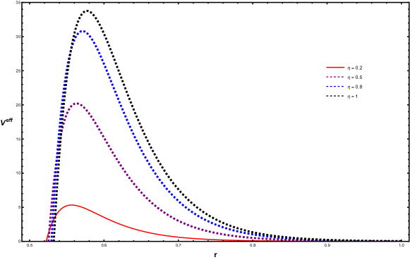
Figure 1: The illustration of $V^{(eff)}$ as a function of $r$ for $Q=0.5$,  $\Lambda=0.01$ and different values of $\eta$.

Fig. 1 demonstrates the behavior of the effective potential for the photon moving in the EMSG charged black hole spacetime as a function of the radial coordinate $r$ for different values of the parameter $\eta$. From this figure we see that the maximum value of the effective potential increase by increment the values of $\eta$ and in the limit of $r\rightarrow\infty$, the effective potential approaches a constant value. In fact, at large radial distances the effect of $\eta$ tends to zero and GR’s result is recovered.
Among all possible motions of the photons, that is, capturing, scattering and unstable (circular/spherical) orbits, only unstable orbits assume a part in the formation of the black hole shadow. The unstable circular orbits of the photons happen at a distance called the photon sphere radius $r_{ph}$ which corresponds with the maximum value of the effective potential and can be determined by the following equations

$$V^{(eff)}|_{r_{ph}}=0=\frac{dV^{(eff)}}{dr}|_{r_{ph}},\quad\quad\mathcal{R}(r)|_{r_{ph}}=\frac{dR(r)}{dr}|_{r_{ph}}=0\,.$$ (39)

It is worth mentioning that since the strong gravitational field in the vicinity of the black hole causes the gravitational lensing, the boundary of the black hole shadow does not occur at the unstable photon orbits, but at the apparent shape of the unstable photon orbits. Subsequently, the radius $r_{ph}$ of the photon sphere for EMSG charged black hole is the smallest value of the roots of the following equation

$$b^{\prime}Ah-2bA^{\prime}h-bAh^{\prime}+2bhA^{\prime}=0\,.$$ (40)

In which prime denotes the derivative respect to $r$. This smallest root can be obtained numerically as can be seen in what follows.

VI GEOMETRICAL SHAPE OF THE SHADOW OF EMSG CHARGED BLACK HOLE

The apparent shape of a black hole is completely distinguishable by the constraint on its shadow. The photons moving in unstable orbits around a black hole form shadow which appears as two dimensional perfect dark disc for a spherically symmetric black hole. The size and shape of a shadow can be determined by geometrical optics considerations. For this purpose, we introduce two impact parameters $a$ and $b$ to characterize a photon near the black hole. These impact parameters are defined as follows

$$a=\frac{L}{E}\,,\quad\quad b=\frac{\mathcal{K}}{E^{2}}\,.$$ (41)

Therefore, we can rewrite $V^{(eff)}$ and $\mathcal{R}(r)$ as functions of these impact parameters as follows

$$V^{(eff)}=\Big{\{}\frac{b(r)}{h}(a^{2}+b)-1\Big{\}}\frac{E^{2}}{A^{2}}\,,\quad\quad\mathcal{R}(r)=\Big{\{}-(a^{2}+b)hb(r)+h^{2}\Big{\}}\frac{E^{2}}{A^{2}}\,.$$ (42)

Having $V^{(eff)}$ and $\mathcal{R}(r)$, through equation (39) we obtain the following equation governing the parameters $a$ and $b$

$$a^{2}+b=\frac{2hh^{\prime}A^{2}-2AA^{\prime}h^{2}}{h^{\prime}bA^{2}+hb^{\prime}A^{2}-hb2AA^{\prime}}\,,$$ (43)

where the radius of the photon sphere is obtained from equation (40). In order to visualize the geometrical shape of the shadow on the observer’s frame, it is convenient to employ the celestial coordinates $\chi$ and $\zeta$ which are defined as Vazquez2004

$$\chi=\lim_{r_{o}\rightarrow\infty}(\frac{r^{2}_{o}p^{\phi}}{p^{t}})=\frac{-a}{\sin\theta}\,,$$ (44)

and

$$\zeta=\lim_{r_{o}\rightarrow\infty}(\frac{r^{2}_{o}p^{\theta}}{p^{t}})=\pm\sqrt{b-a^{2}\cot(\theta)}\,,$$ (45)

in which $r_{o}$ is the distance between the black hole and a far distant observer and $[p^{t},p^{\theta},p^{\phi}]$ are the tetrad components of the momentum. Fig. 2 shows a schematic of the celestial coordinates used in this setup.

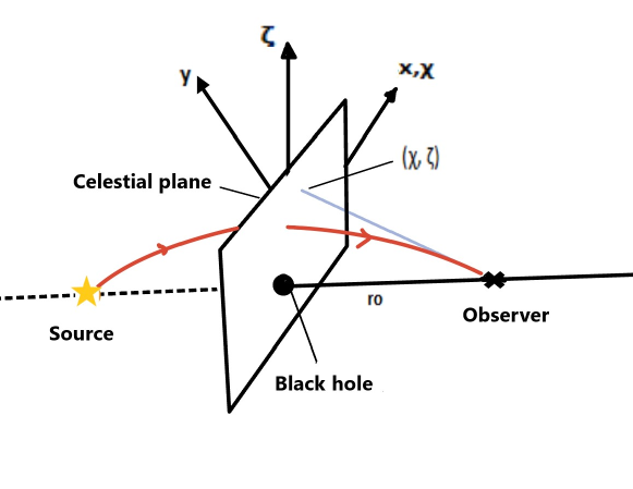
Figure 2: The schematic diagram of celestial coordinates from observer sight located far from the black hole in the position $(r_{o},\frac{\pi}{2})$, where $r_{o}$ determines the distance from the black hole and $\frac{\pi}{2}$ is the angular coordinate for the observer. The coordinates $(\chi,\zeta)$ are the apparent distances of the image from the symmetry axis and from its projection on the equatorial plane, respectively.

One can see where $\theta=\frac{\pi}{2}$ (equatorial plane), then $\chi=-a$ and $\zeta=\pm\sqrt{b}$. Accordingly, we reach at the following result

$$R_{s}^{2}=a^{2}+b=\chi^{2}+\zeta^{2}\,,$$ (46)

where $R_{s}$ is the shadow radius in celestial coordinates; the shadow of which appears as a circle. In table 1 we collect some computed numerical results for the event horizon ($r_{h}$), cosmological horizon ($r_{c}$), photon sphere radius $r_{ph}$ and shadow radius $R_{s}$ for an EMSG charged black hole.

Based on the numerical results provided in table 1, we draw a contour plot of the equation (46). Fig. 3 demonstrates the geometrical shapes of the shadow of the EMSG charged black hole for $\Lambda=0.01$ in celestial coordinates. Fig. (3a) shows the shadow of the EMSG charged black hole for different values of the parameter $\eta$. This figure shows that the shadow size for different values of the parameter $\eta$ approach each other. Fig. (3b) is an illustration of the shadow of the EMSG charged black hole for different values of parameter $Q$. From Fig. (3a) we see that by enhancing the effect of the electric charge, the shadow size decreases accordingly. About the role of the cosmological constant on the shadow, generally the shadow angle decreases by increasing the value of the cosmological constant so that the shadow angle decreases faster for the larger values of the cosmological constant in this setup. To see more details about the influence of the cosmological constant on the shadow of a black hole we refer to Perlick2018 ; Firouzjaee2019 . As has been shown in Ref. Perlick2018 , the angular radius of the shadow of a Schwarzschild-de Sitter black hole shrinks to a non-zero finite value if the comoving observer approaches infinity. So, the limit of infinity in Eqs. (41) and (42) is defined for an observer who is comoving with the cosmic expansion.

Table 1: The computed numerical values for $r_{h}$, $r_{ph}$, $r_{c}$ and $R_{s}$ of EMSG charged Black hole for different values of the parameters $Q$ and $\eta$

Q = 0.1							$\eta=0.01$
$\eta$	$0.01$	$0.02$	$0.03$	$0.04$	$0.05$	$0.06$	$Q$	0.01	0.1	0.2	0.3
$r_{h}$	1.98	2	2.03	2.05	2.07	2.1	$r_{h}$	2.05	1.98	1.75	0.473
$r_{ph}$	2.94	2.98	3.01	3.04	3.07	3.11	$r_{ph}$	3.03	2.94	2.65	1.321
$r_{c}$	16.1	16	15.9	15.8	15.7	15.6	$r_{c}$	16.1	16.1	16.1	16.2
$R_{s}$	5.46	5.55	5.65	5.74	5.85	5.95	$R_{s}$	5.54	5.46	5.10	4.17

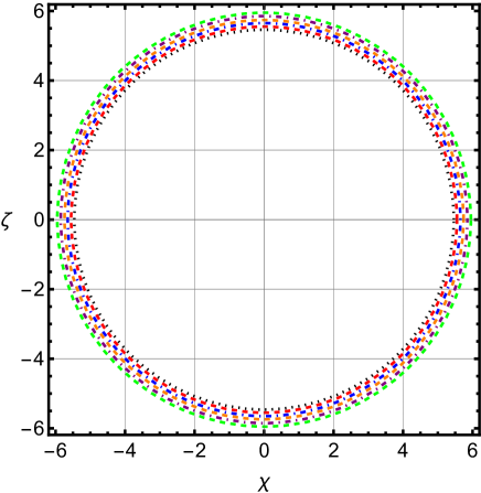
(a) Q=0.1

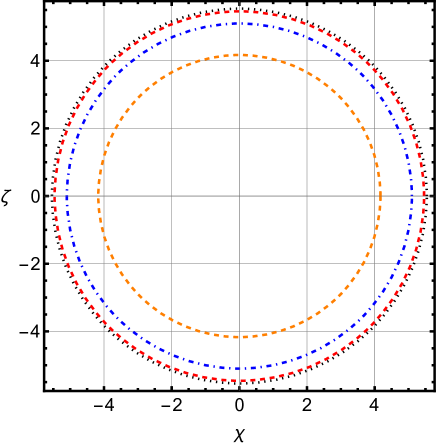
(b) $\eta$=0.01

Figure 3: Contour plot of geometrical shape of EMSG charged black hole in celestial coordinate with $\Lambda=0.01$

VII CONSTRAINTS FROM EHT OBSERVATION OF Sgr A^∗

In this section we compare our results of the shadow size of the EMSG charged black hole with the recent image of the supermassive black hole Sgr A* released by the EHT Collaboration. Indeed, we investigate the possible constraints on the Energy-Momentum Squared Gravity by utilizing the EHT provided data. The captured image by EHT collaboration delivered through the Very Long Baseline Interferometry (VLBI), shows a bright emission ring surrounding a central dark spot. It is interesting to note that very recently EHT collaboration has revealed strong magnetic fields spiraling at the edge of Milky Way’s central black hole, Sgr A* EHT2024 , the observation of which in some sense supports the idea to study charged version of the EMSG black holes in the present manuscript. We can use the size of the bright ring to estimate the size of the black hole shadow under two circumstances: $i$) A bright source of light exists that its light strongly bends near the horizon, and $ii$) The surrounding emission region is geometrically thick and optically thin at the VLBI network wavelength Vagnozzi2022moj .
For this purpose, first we need the mass-to-distance ratio of Sgr A*. These two quantities have been measured by two sets of instruments/teams, “Keck” and “VLTI”. They found their results through the stellar cluster dynamics model by S$0-2$ star which is shown in table 2 at the $68$$\%$ level of confidence Doetal2019 ,Abuter2020 .

Table 2: Mass and distance of Sgr A* estimated via Keck and VLTI instruments.

Survey	$M(\times 10^{6}M_{\odot})$	$D(kpc)$
$Keck$	3.951 ± 0.047	7.953 ± 0.050 ± 0.032
$VLTI$	4.297 ± 0.012 ± 0.040	8.277 ± 0.009 ± 0.033

The second requirement is the calibration factor to link the size of the bright emission ring with the size of the corresponding shadow which tells us how reliable it is to use the size of the bright ring of emission as an indicator of the shadow size. Several sources of uncertainties e.g. formal measurement uncertainties, fitting/model uncertainties, theoretical uncertainties pertaining to the emissivity of the plasma Vagnozzi2022moj (see the original discussion in Sec. 3 of Ref. Akiama2022 ), produce the calibration factor. The EHT conducts the calibration factor with uncertainties in Sgr A*’s mass-to-distance ratio, and the angular diameter of Sgr A*’s bright ring of emission by carefully examining different sources of uncertainties Akiama2022 . The fractional deviation between the deduced shadow radius $r_{sh}$ and the shadow radius of a Schwarzschild black hole of angular size $\theta$ ($\theta_{sh}=3\sqrt{3}\theta_{g}$), $r_{sh,Schwarzschild}=3\sqrt{3}M$ reads $\delta$ which are collected by EHT. In practice $\delta$ is given as follows Vagnozzi2022moj

$$\delta=\frac{r_{sh}}{r_{sh,Schwarzschild}}-1=\frac{r_{sh}}{3\sqrt{3}M}-1\,.$$ (47)

Based on Keck and VLTI measurements of the mass-to-distance ratio, $\delta$ will be estimated as $0.04^{+0.09}_{-0.10}$ for Keck and $0.08^{+0.09}_{-0.09}$ for VLTI. For simplicity, one can take the average of the Keck and VLTI-based estimates of $\delta$ that leads to the following approximate value

$$\delta\simeq-0.060\pm 0.065\,.$$ (48)

Under the assumption of Gaussianity, this gives easily the following $1\sigma$ and $2\sigma$ ranges for $\delta$

$$\begin{split}-0.125&\leq\delta\leq 0.005\quad(1\sigma)\,,\\ -0.19&\leq\delta\leq 0.07\quad(2\sigma)\,.\end{split}$$ (49)

According to the Keck and VLTI estimations, we sense that Sgr A*’s shadow is slightly smaller than the expected $3\sqrt{3}M$ for a Schwarzschild black hole with the same mass, with a $\leq 68$$\%$ level of confidence preference for $\delta<0$. By assuming Gaussian uncertainties, one can consider equation (47) and inverting $r_{sh}/M=3\sqrt{3}(\delta+1)$ to find the following $1\sigma$ and $2\sigma$ limits on $r_{sh}/M$:

$$\begin{split}4.55&\leq r_{sh}/M\leq 5.22\quad(1\sigma)\,,\\ 4.21&\leq r_{sh}/M\leq 5.56\quad(2\sigma)\,.\end{split}$$ (50)

Now we utilize the limits in equations (50) to compare the shadow of the EMSG charged black hole with Sgr A*’s shadow. Fig. 4 illustrates the behavior of the shadow radius of the EMSG charged black hole in comparison with the EHT’s shadow size of Sgr A* within $1\sigma$ and $2\sigma$ levels of confidence. The gray and light gray areas are compatible with the EHT image of Sgr A* at $1\sigma$ and $2\sigma$ levels of confidence respectively, after taking into account the Keck and VLTI average mass-to-distance ratio for Sgr A*. More than $2\sigma$ uncertainties are excluded regions by the same observations. In Fig. 4a, we plotted the shadow radius of EMSG charged black hole as a function of $\eta$ for $Q=0.1$ and $\Lambda=0.01$. As it is clear, for $\eta\leq 0.02$ the EMSG charged black hole shadow radius is compatible with Sgr A* in $2\sigma$ level of confidence. According to Fig. 4b, for $\eta=0.01$ and $\Lambda=0.01$ in the interval $0.01\leq Q\leq 0.16$ the shadow radius of the EMSG charged black hole stays within the $2\sigma$ limit. In the interval $0.16\leq Q\leq 0.26$, the shadow radius of the EMSG charged black hole satisfies the $1\sigma$ confidence level of the EHT observations. Therefore, the Sgr A* can be an EMSG charged black hole in an accelerating universe ($\Lambda=0.01$) in the units of $\eta=0.01$, $Q=0.1$.

(a) Q=0.1

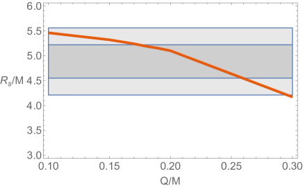
(b) $\eta$=0.01

Figure 4: The shadow radius of an EMSG charged black hole in units of the black hole mass $M$.

VIII ENERGY EMISSION RATE

Hawking radiation is a phenomenon that allows black holes to emit radiation through the quantum fluctuation process. In fact inside the black hole and near the horizon, quantum fluctuations create and annihilate many pairs of particles-antiparticles. In this regard, particles with positive energy can escape from the black hole through a quantum tunneling process, which can lead the black hole to radiate and evaporate gradually. The associated energy emission rate can be expressed as follows wei2013

$$\frac{d^{2}E(\omega)}{d\omega dt}=\frac{2\pi^{2}\sigma_{lim}}{\exp(\omega/T)-1}\omega^{3}\,,$$ (51)

in which $\omega$ is the emission frequency and $T$ is the Hawking temperature of the event horizon which we obtain as

$$T=\frac{(5Mr_{h}^{5}+4\pi(3q^{4}-5q^{2}r_{h}^{4}))\kappa}{80\pi^{2}r_{h}^{7}}-\frac{2r_{h}\Lambda}{3}\,.$$ (52)

In the high energy limit, the absorption cross section oscillates around a limiting constant value $\sigma_{lim}$ which is approximately equal to the photon sphere or black hole shadow. This value reads as (see Refs. Decanini2011 ; Decanini2011a ; Mashhoon1973 )

$$\sigma_{lim}\approx\pi R_{s}^{2}\,,$$ (53)

where $R_{s}^{2}$ is the black hole shadow radius (46).

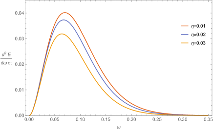
(a) Q=0.1

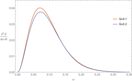
(b) $\eta$=0.01

Figure 5: The graph of energy emission rate as function of $\omega$ for EMSG charged black hole

Fig. (5)is the illustration of the energy emission rate form a EMSG charged black hole as a function of $\omega$. In Fig. (5a) we plotted the energy emission rate of the EMSG charged black hole for different values of the parameter $\eta$ by setting $Q=0.1$. We find out that increment of $\eta$ decreases the energy emission rate for the EMSG charged black hole. So, the evaporation of the EMSG charged black hole decelerates by growth of the parameter $\eta$. Fig. (5b) shows the energy emission rate from a EMSG charged black hole for different values of the charge parameter $Q$, when $\eta$ is fixed. We see that the energy emission rate for the EMSG charged black hole will decrease, which means that the EMSG charged black hole evaporates faster for the smaller values of the electric charge.

IX SUMMERY AND CONCLUSION

In this work we have investigated the shadow cast formed by an EMSG charged black hole in confrontation with EHT data of Sgr A*. We started by focusing on the motion and trajectories of photons in the background of an EMSG charged black hole. In non-linear electrodynamics, photons move along geodesics that are null in the effective metric. Therefore, we first obtained the effective metric for an EMSG charged black hole. For this purpose, we utilized the Hamilton-Jacobi method and Carter constant to find complete equations of motion for photons’ trajectories, and derivation of the corresponding effective potential. Then, by introducing appropriate celestial coordinates and by deriving the effective potential to calculate the radius of the possible circular orbits, we demonstrated the shadow shape of EMSG charged black hole by some constructive contour plots. Indeed, we plotted the shadow shape of the EMSG charged black hole in celestial coordinate for positive values of the cosmological constant to fulfill the late time cosmic speed up. We have shown that for a given electric charge, the shadow size of the EMSG charged black hole varies effectively for different values of the parameter $\eta$. We also found out that for a fixed value of $\eta$, the shadow size increases by increasing the electric charge. Then we used EHT data to evaluate and justify our results of the shadow shape in confrontation with Sgr A* data. As a result and within the parameter space of the present model, the Sgr A* can be an EMSG charged black hole in an accelerating universe (for instance, with $\Lambda=0.01$, $\eta=0.01$ and $Q=0.1$). We have constrained the parameter $\eta$ and the electric charge by comparing the shadow size reported by EHT for Sgr A* with the shadow radius of the EMSG charged black hole calculated in this paper. We found that for a fixed value of the electric charged, the shadow radius of the EMSG charged black hole for $0.01\leq\eta\leq 0.02$ lies within the $2\sigma$ confidence level of the Sgr A* shadow radius. We also noticed that for $\eta=0.01$ , the range for the electric charge of EMSG charged black hole to be compatible with the EHT data of Sgr A* has to be $0.01\leq Q\leq 0.3$. Furthermore, we explored the energy emission rate for the EMSG charged black hole in this setup. We observed that for smaller amounts of the electric charge and the parameter $\eta$, the EMSG charged black hole evaporates faster. As EHT collaboration has reported very recently, strong magnetic fields are spiraling at the edge of Milky Way’s central black hole, Sgr A* EHT2024 . This novel observation highlights the role of magnetic field in black hole spacetime which in some sense supports the idea to study charged version of the EMSG black holes in this study.

Acknowlegment

we appreciate Dr sara saghafi for fruitful discussion.

References

- (1) K. Akiyama et al. [Event Horizon Telescope], Astrophys. J. Lett. 875, L1 (2019) [arXiv:1906.11238 [astro-ph.GA]].
- (2) K. Akiyama et al. [Event Horizon Telescope], Astrophys. J. Lett. 875, L2 (2019) [arXiv:1906.11239 [astro-ph.GA]].
- (3) K. Akiyama et al. [Event Horizon Telescope], Astrophys. J. Lett. 875, L3 (2019) [arXiv:1906.11240 [astro-ph.GA]].
- (4) K. Akiyama et al. [Event Horizon Telescope], Astrophys. J. Lett. 875, L4 (2019) [arXiv:1906.11241 [astro-ph.GA]].
- (5) K. Akiyama et al. [Event Horizon Telescope], Astrophys. J. Lett. 875, L5 (2019) [arXiv:1906.11242 [astro-ph.GA]].
- (6) K. Akiyama et al. [Event Horizon Telescope], Astrophys. J. Lett. 875, L6 (2019) [arXiv:1906.11243 [astro-ph.GA]].
- (7) K. Akiyama et al. [Event Horizon Telescope], Astrophys. J. Lett. 930, L12 (2022).
- (8) K. Akiyama et al. [Event Horizon Telescope], Astrophys. J. Lett. 930, L13 (2022).
- (9) K. Akiyama et al. [Event Horizon Telescope], Astrophys. J. Lett. 930, L14 (2022).
- (10) K. Akiyama et al. [Event Horizon Telescope], Astrophys. J. Lett. 930, L15 (2022).
- (11) L. Barack et al., Class. Quant. Grav. 36, no.14, 143001 (2019). [arXiv:1806.05195 [gr-qc]].
- (12) K. Schwarzschild, Sitzungsber. Preuss. Akad. Wiss. Berlin, (Math. Phys. ) 1916, 189 (1916). [arXiv:physics/9905030].
- (13) R. Penrose, Phys. Rev. Lett. 14, 57 (1965). [arXiv:physics/9905030].
- (14) C. Bambi, Annalen Phys. 530, 1700430 (2018). [arXiv:1711.10256 [gr-qc]].
- (15) V. Perlick, [arXiv:1010.3416 [gr-qc]].
- (16) J. L. Synge, Mon. Not. Roy. Astron. Soc. 131, 463 (1966).
- (17) J. P. Luminet, Astron. Astrophys. 75, 228 (1979).
- (18) V. Perlick and O. Yu. Tsupko, Physics Reports, 947, 1-39 (2022).
- (19) M. Wang, S. Chen and J. Jing, Commun. Theor. Phys. 74, 097401 (2022).
- (20) D. Ayzenberg et al., Fundamental Physics Opportunities with the Next-Generation Event Horizon Telescope, [arXiv:2312.02130].
- (21) K. Akiyama et al. [Event Horizon Telescope], Astrophys. J. Lett. 875, L12 (2021) [arXiv:2105.01169 [astro-ph.GA]].
- (22) K. Akiyama et al. [Event Horizon Telescope], Astrophys. J. Lett. 910, L13 (2021) [arXiv:2105.01173 [astro-ph.GA]].
- (23) K. Akiyama et al. [Event Horizon Telescope], Astrophys. J. Lett. 930, L16 (2022).
- (24) K. Akiyama et al. [Event Horizon Telescope], Astrophys. J. Lett. 930, L17 (2022).
- (25) K. Akiyama et al. [Event Horizon Telescope], Astrophys. J. Lett. 964, L25 (2024).
- (26) K. Akiyama et al. [Event Horizon Telescope], Astrophys. J. Lett. 964, L26 (2024).
- (27) H. C. D. L. Junior, P. Cunha, V.P., C. A. R. Herdeiro and L. C. B. Crispino, Phys. Rev. D. 104 no.4,044018 (2021).
- (28) M. Okyay and A. vgn, JCAP 01 no.01, 009 (2022).
- (29) Z. Hu, Z. Zhong, P. C. Li, M. Guo and B. Chen,Phys. Rev. D 103, no.4, 044057 (2021).
- (30) Z. Zhong, Z. Hu, H. Yan, M. Guo and B. Chen, Phys. Rev. D 104, no.10, 104028 (2021).
- (31) A. Allahyari, M. Khodadi, S. Vagnozzi and D. F. Mota, JCAP 02 (2020), 003.
- (32) Eric Poisson and Clifford M. Will, Gravity: Newtonian, Post-Newtonian, Relativistic (Cambridge University Press, Cambridge, 2014).
- (33) S. Nojiri and S. D. Odintsov, Int. J. of Geom. Methods in Mod. Phys. 4 115 (2007).
- (34) A. De Felice and S. Tsujikawa, Living Reviews in Relativity. 13 (1): 3 (2010), [arXiv:1002.4928].
- (35) S. Nojiri and S. D. Odintsov, Phys. Rep. 505 59 (2011).
- (36) S. Capozziello and M. De Laurentis, Phys. Rept. 509, 167 (2011).
- (37) S. Nojiri, S. D. Odintsov and V. K. Oikonomou, Phys. Rept. 692 1-104 (2017).
- (38) N. Katirci and M. Kavuk, Eur. Phys. J. Plus 129, 163 (2014).
- (39) M. Roshan and F. Shojai, Phys. Rev. D 94, no.4, 044002 (2016) [arXiv:1607.06049 [gr-qc]].
- (40) M. Born and L. Infeld, Proc. Roy. Soc. Lond. A 144, 425 (1934).
- (41) J. Plebansky, in Lectures on Nonlinear Electrodynamics Ed. Nordita, Copenhagen, (1968).
- (42) W. Dittrich and H. Gies, Phys. Rev. D 58, 025004 (1998).
- (43) R. G. Cai, D. W. Pang and A. Wang, Phys. Rev. D 70, 124034 (2004).
- (44) J. Y. Kim, Deection of light by magnetars in the generalized Born-Infeld electrodynamics, [arXiv:2202.11913 [gr-qc]].
- (45) M. Sharif and M. Zeeshan Gul, Chin. J. Phys. 80, 58-73 (2022) doi:10.1016/j.cjph.2022.06.016 [arXiv:2306.10117 [gr-qc]].
- (46) S. A. Hosseini Mansoori, F. Felegary, M. Roshan, O. Akarsu and M. Sami, [arXiv:2306.09181 [gr-qc]].
- (47) M. Sharif and M. Zeeshan Gul, Phys. Scripta 96, no.12, 125007 (2021) doi:10.1088/1402-4896/ac2378 [arXiv:2305.09658 [gr-qc]].
- (48) Á. J. C. Canuto and A. F. Santos, Eur. Phys. J. C 83, no.5, 404 (2023) doi:10.1140/epjc/s10052-023-11570-3 [arXiv:2305.01388 [gr-qc]].
- (49) M. Sharif and S. Naz, Annals Phys. 451, 169240 (2023) doi:10.1016/j.aop.2023.169240 [arXiv:2304.06732 [gr-qc]].
- (50) B. Farsi, A. Sheykhi and M. Khodadi, Phys. Rev. D 108, no.2, 023524 (2023) doi:10.1103/PhysRevD.108.023524 [arXiv:2304.01571 [astro-ph.CO]].
- (51) E. Nazari, Phys. Rev. D 105, no.10, 104026 (2022) doi:10.1103/PhysRevD.105.104026 [arXiv:2204.11003 [gr-qc]].
- (52) E. Nazari, M. Roshan and I. De Martino, Phys. Rev. D 105, no.4, 044014 (2022) doi:10.1103/PhysRevD.105.044014 [arXiv:2201.08578 [gr-qc]].
- (53) M. Faraji, N. Rashidi and K. Nozari, Eur. Phys. J. Plus 137, no.5, 593 (2022) doi:10.1140/epjp/s13360-022-02820-6 [arXiv:2107.13547 [gr-qc]].
- (54) M. Sharif and M. Zeeshan Gul, Eur. Phys. J. Plus 136, 503 (2021) [arXiv:2105.04416 [gr-qc]].
- (55) S. Shahidi, Eur. Phys. J. C 81, no.4, 274 (2021) doi:10.1140/epjc/s10052-021-09082-z [arXiv:2104.07931 [gr-qc]].
- (56) M. Sharif and M. Zeeshan Gul, Phys. Scripta 96, no.2, 025002 (2021) doi:10.1088/1402-4896/abcd67 [arXiv:2103.03083 [gr-qc]].
- (57) C. Ranjit, P. Rudra and S. Kundu, Annals Phys. 428, 168432 (2021) doi:10.1016/j.aop.2021.168432 [arXiv:2010.02753 [gr-qc]].
- (58) P. Rudra and B. Pourhassan, Phys. Dark Univ. 33, 100849 (2021) doi:10.1016/j.dark.2021.100849 [arXiv:2008.11034 [gr-qc]].
- (59) E. Nazari, F. Sarvi and M. Roshan, Phys. Rev. D 102, no.6, 064016 (2020) doi:10.1103/PhysRevD.102.064016 [arXiv:2008.06681 [gr-qc]].
- (60) K. N. Singh, A. Banerjee, S. K. Maurya, F. Rahaman and A. Pradhan, Phys. Dark Univ. 31, 100774 (2021) doi:10.1016/j.dark.2021.100774 [arXiv:2007.00455 [gr-qc]].
- (61) S. Bhattacharjee and P. K. Sahoo, Eur. Phys. J. Plus 135, no.1, 86 (2020) doi:10.1140/epjp/s13360-020-00116-1 [arXiv:2001.06569 [gr-qc]].
- (62) A. Kazemi, M. Roshan, I. De Martino and M. De Laurentis, Eur. Phys. J. C 80, no.2, 150 (2020) doi:10.1140/epjc/s10052-020-7662-y [arXiv:2001.04702 [gr-qc]].
- (63) A. H. Barbar, A. M. Awad and M. T. AlFiky, Phys. Rev. D 101, no.4, 044058 (2020) doi:10.1103/PhysRevD.101.044058 [arXiv:1911.00556 [gr-qc]].
- (64) C. Y. Chen and P. Chen, Phys. Rev. D 101, no.6, 064021 (2020) doi:10.1103/PhysRevD.101.064021 [arXiv:1910.12262 [gr-qc]].
- (65) S. Bahamonde, M. Marciu and P. Rudra, Phys. Rev. D 100, no.8, 083511 (2019) doi:10.1103/PhysRevD.100.083511 [arXiv:1906.00027 [gr-qc]].
- (66) Ö. Akarsu, J. D. Barrow, C. V. R. Board, N. M. Uzun and J. A. Vazquez, Eur. Phys. J. C 79, no.10, 846 (2019) doi:10.1140/epjc/s10052-019-7333-z [arXiv:1903.11519 [gr-qc]].
- (67) O. Akarsu, N. Katirci, S. Kumar, R. C. Nunes and M. Sami, Phys. Rev. D 98, no.6, 063522 (2018) doi:10.1103/PhysRevD.98.063522 [arXiv:1807.01588 [gr-qc]].
- (68) N. Nari and M. Roshan, Phys. Rev. D 98, no.2, 024031 (2018) doi:10.1103/PhysRevD.98.024031 [arXiv:1802.02399 [gr-qc]].
- (69) Ö. Akarsu, J. D. Barrow, S. Çıkıntoğlu, K. Y. Ekşi and N. Katırcı, Phys. Rev. D 97, no.12, 124017 (2018) doi:10.1103/PhysRevD.97.124017 [arXiv:1802.02093 [gr-qc]].
- (70) C. V. R. Board and J. D. Barrow, Phys. Rev. D 96, no.12, 123517 (2017) [erratum: Phys. Rev. D 98, no.12, 129902 (2018)] doi:10.1103/PhysRevD.96.123517 [arXiv:1709.09501 [gr-qc]].
- (71) M. Novello, V. A. De Lorenci, J. M. Salim and R. Klippert, Phys. Rev. D 61, 045001 (2000).
- (72) E. G. de Oliveira Costa and S. E. Perez Bergliaffa, Class. Quant. Grav. 26, 135015 (2009).
- (73) B. Carter, Phys. Rev. 174, 1559-1571 (1968).
- (74) V. Perlick, O. Yu. Tsupko, G. S. Bisnovatyi-Kogan, Phys. Rev. D 97, 104062 (2018), [arXiv:1804.04898 [gr-qc]].
- (75) J. T. Firouzjaee and A. Allahyari, Eur. Phys. J. C 79, 930 (2019), [arXiv:1905.07378 [astro-ph.CO]].
- (76) S. E. Vazquez and E. P. Esteban, Nuovo Cim. B 119, 489-519 (2004)) [arXiv:0308023 [gr-qc]].
- (77) S. Vagnozzi, R. Roy, Y. D. Tsai, L. Visinelli, M. Afrin, A. Allahyari, P. Bambhaniya, D. Dey, S. G. Ghosh and P. S. Joshi, Class. Quant. Grav. 40, no.16, 165007 (2023) [arXiv:2205.07787 [gr-qc]].
- (78) EHT Collaboration, “Astronomers unveil strong magnetic fields spiraling at the edge of Milky Way’s central black hole”. www.eso.org. Retrieved March 27, 2024.
- (79) T. Do et al., Science 362, 664 (2019) [arXiv:1907.10731 [gr-qc]].
- (80) R. Abuter et al. (GRAVITY), Astron. Astrophys. 636, L5 (2020) [arXiv:2004.07187 [astro-ph.GA]].
- (81) K.Akiama et al. (Event Horizon Telescope), Astrophys. J. Lett. 930, L17 (2022) [arXiv:2004.07187 [astro-ph.GA]].
- (82) S. W. Wei and Y. X. Liu, J. Cosmol. Astropart. Phys. 11, 063 (2013)) [arXiv:1311.4251 [gr-qc]].
- (83) B. Mashhoon, Phys. Rev. D 7, 2807 (1973).
- (84) Y. Decanini, A. Folacci and B. Raffaelli, Class. Quant. Grav. 28, 175021 (2011) [arXiv:1104.3285 [gr-qc]].
- (85) Y. Decanini, G. Esposito-Farese and A. Folacci, Phys. Rev. D 83, 044032 (2011) [arXiv:1311.4251 [gr-qc]].