Cluster Formation of Free and Congested Flows in Urban Road Networks

Abstract

Understanding traffic behavior is crucial for enhancing the stable functioning and safety of transportation systems. Previous percolation-based transportation studies have analyzed transition behaviors from free-flow to traffic-jam states, with a focus on robustness and resilience during congestion. However, relatively less attention is paid to the percolation analysis of the free-flow states, specifically how free-flow clusters form and grow. In this study, we investigate the percolation patterns of two opposing traffic scenarios—traffic jam state and free-flow state—within the same road network using Chengdu taxi data and compare their percolating behaviors. Our analysis reveals differences between the two scenarios in the growth patterns of the giant connected component (GCC), which is captured by a persistent gap between the GCC size curves, particularly during peak hours. We attribute these disparities to a long-range spatial correlation of traffic speed within a road network. Empirically, we find distinct long-range spatial correlations in traffic, using rescaled taxi speeds on roads, and we examine their relationship with each percolation pattern. Our analysis provides an integrated view of traffic dynamics and uncovers intrinsic traffic correlations within urban areas that drive these intriguing percolation patterns. Our findings also offer valuable metrics for effective traffic management and accident prevention strategies, aligning with urban transportation safety and reliability goals. These insights are beneficial for assessing and designing resilient urban road networks that maintain functionality under stress, ultimately improving the reliability of traffic assessments and reducing accidents.

1 Introduction

In the study of urban road systems, improving traffic flow and reducing congestion are critical challenges. Understanding these temporal behaviors such as traffic flow and congestion is crucial to optimizing urban mobility, minimizing traffic accidents, and improving overall road safety and reliability of traffic management systems. The complexity of traffic flows within road networks arises from the intricate interplay of countless vehicle movements. These movements are driven by people’s travel purposes [1, 2], the geographical and structural characteristics of the embedded road network [3, 4, 5], and other diverse factors [6, 7]. Statistical physics, which is adept at analyzing complex multi-particle systems, has been widely applied to elucidate these traffic dynamics [8, 9]. Complex network analysis offers powerful tools for examining collective behavior emerging from interactions within diverse transportation infrastructure systems, particularly macroscopic traffic phenomena in road networks [10, 11, 12, 13].

Traffic congestion is conceptualized as a cascading phenomenon, where a localized disruption (such as an accident, sudden lane closure, or natural crowdedness) can propagate through nearby roads, triggering a chain reaction of slowdowns. Concurrently, traffic conditions exhibit intrinsic spatial correlations among neighboring road segments [14, 15]. Moreover, in urban transportation systems, local traffic clusters frequently diffuse and form global congestion, in which long-range correlation has been observed [16, 17]. Numerous previous studies have investigated these congestion formation processes using network percolation analysis [2, 18, 19, 20, 21, 22], suggesting unique percolation behaviors found in urban traffic networks. In particular, many studies highlight the crucial role of long-range correlation in road networks for the emergence of global congestion [15, 22, 23, 24].

Previous traffic percolation analyses have mainly followed two approaches: one examines the growth patterns of congested road clusters [20], while the other investigates the breakdown patterns of free-flow clusters (the remaining network after removing congested roads) [21]. The former represents how congestion arises and spreads spatially throughout the network, while the latter describes the robustness of the network structure when roads become non-functional due to congestion. Although these two percolating clusters illuminate different aspects of traffic configuration, both processes share a common focus on the jamming process. Furthermore, by applying this percolation analysis of traffic congestion, various indices—such as connectivity, resilience, and robustness—have been developed and systematically measured to evaluate urban road networks and traffic dynamics [25]. However, the process of smooth traffic formation remains less explored despite its crucial importance in terms of stable management, compared to the significant attention paid to the formation of congestion in traffic.

This study addresses this gap by simultaneously examining both the formation of free-flow clusters and traffic-jam clusters within a given traffic configuration. This simultaneous observation is essential for understanding urban road networks and thus enhancing the reliability of traffic evaluation systems because both phenomena occur concurrently and interact with each other. By analyzing these cluster formations together, we gain a more comprehensive view of dynamic traffic patterns in urban environments, allowing a more accurate assessment and prediction of traffic conditions. Using taxi data [26] from Chengdu, China, we provide insights into the underlying mechanisms that can inform more resilient urban planning. We take snapshots of the traffic distribution at specific times and perform percolation analysis, occupying road segments in order of their speed (high to low or vice versa). This dual analysis of traffic-jam and free-flow processes reveals crucial insights into the multifaceted features of traffic structure.

Implementing these findings can lead to better traffic management systems that minimize congestion and reduce accident rates, significantly contributing to urban safety. For instance, a robust and resilient traffic spatial structure can be understood as one generating smaller, scattered traffic-jam clusters and well-connected, larger free-flow clusters at a given traffic level. This integrated analysis using various metrics can help design more effective traffic evaluation systems. Our analysis employs road network data and high-resolution taxi traffic data from Chengdu. By exploring different cluster formation patterns of the two percolation processes, we empirically investigate the relationship between the spatial correlation of traffic and percolating patterns. Additionally, we observe how these patterns change between different time windows, highlighting the distinct disparity between rush hour and non-rush hour periods.

In the following section, we provide a brief introduction to the Chengdu road network and Chengdu taxi dataset used in this study, as well as an explanation of the methods for inputting traffic conditions and traffic percolation (Sec. 2). Next, in Sec. 3.1, we present an explanation and analysis of the properties of traffic-jam and free-flow percolation and their difference. In Sec. 3.2, we conduct correlation analysis in the context of urban transportation. Finally, the section concludes with a summary of the research and a discussion of the findings.

2 Percolating Clusters in Traffic Assessment and Data Description

2.1 Traffic-jam and free-flow percolation

Table 1: Notation used in this paper. the notation “Network” describes the network structure, while “Percolation” refers to quantities obtained after applying the percolation process.

Network
$V$, $E$	a set of nodes (intersections) and a set of directed links (roads)
$W(t)$	a set of link weights at time $t$
$G[V,E,W(t)]$	the weighted directed traffic road network at time $t$
$N$, $L$	the number of nodes, $N=|V|$, and the number of directed links, $L=|E|$
$r_{i}(t)$	the rescaled average speed of taxies on a road $e_{i}\in E$; i.e., $r_{i}(t)\in W(t)$
Percolation
$Q^{\rm(jam)},Q^{\rm(free)}$	the superscript notation; a quantity $Q$ in the traffic-jam (jam) or free-flow (free) cluster
$p,p_{c}$	an occupation fraction of link and the threshold fraction
$s(p;t)$	the relative size $s$ of the giant connected component at occupation fraction $p$ and time $t$
$\Delta A$	the gap area between two curves between $s^{\rm(jam)}(p)$ and $s^{\rm(free)}(p)$
$\alpha$	the exponent representing the long-rangeness of weight-weight correlation.

To assess the traffic condition of urban roads, we adopt the percolation analysis using the traffic of the road and detect the traffic clusters. In doing so, we first construct a road network comprising $N$ nodes (intersections) and $L$ directed links (roads) as an embedding structure. The notations used in this paper were summarized in Table 1.

As an indicator of the traffic status of the road (link) $e_{i}\in E$, the average speed of the vehicle that runs along the road is assigned, but the magnitude itself is quite impractical due to the considerable variation in daily traffic usage patterns (e.g., people normally drive at higher speeds on highways while they tend to drive more slowly in smaller alleyways). Therefore, to ensure the standardized criterion applicable for all roads, we use the rescaled speed, as proposed in previous research [19]. The (average) rescaled speed $r_{i}(t)$ on the link $e_{i}$ at time $t$ is defined as $r_{i}(t)\equiv v_{i}(t)/v_{i}^{\mathrm{max}}$, where $v_{i}(t)$ is the average speed of vehicles on the link $e_{i}$ at time $t$ and $v_{i}^{\mathrm{max}}=\max_{t}v_{i}(t)$ for a given day. This standardized value allows us to express the relative traffic conditions of a given road within the range of 0 to 1, then which becomes the link weight on the link $e_{i}$ at time $t$ in terms of the directed weighted network. We finally achieve time-dependent weighted directed networks $G[V,E,W(t)]$ (note that the rescaled speeds, namely the link weights set $W(t)$ can be varied in time $t$ while the embedding structure $V$ and $E$ remain static).

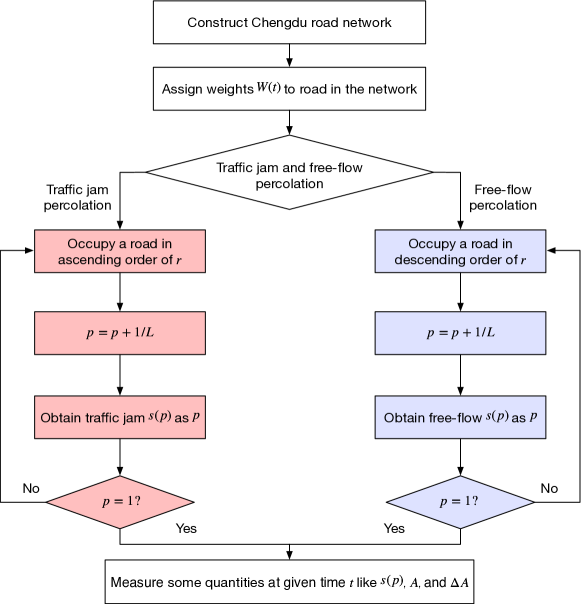
Figure 1: The flowchart describing the traffic percolation processes. The link density (occupation fraction) $p$ in the traffic-jam and free-flow percolation is explicitly $p^{\rm(jam)}$ and $p^{\rm(free)}$, respectively.

Percolation theory has been used ubiquitously in various fields to evaluate the functioning of systems, such as resilience, vulnerability, and robustness [19, 20, 21], so it has been popularly applied to traffic systems to assess the status and conditions of traffic in road networks [27]. In ordinary percolation, a randomly selected node or link is occupied with an occupation probability , possibly leading to the emergence of the giant connected component (GCC). This random occupation is improper in the traffic analysis, so we redesign the weight-based percolation process based on the previous study [19, 26]. The value of $r$ closer to 0 represents a road with poor traffic status (traffic jams), while the value closer to 1 represents good traffic status (free flow). By introducing the link occupation fraction $p$ (not a probability as above) as the control parameter, a link is occupied sequentially according to its weight $r$ in ascending order (low to high $r$) or descending order (high to low $r$). The sequential occupation of the lowest $r$ and highest $r$ corresponds to traffic-jam and free-flow percolation, respectively.

Note that traffic clusters emerge in a deterministic manner due to the absence of stochasticity in the occupation process and that the two types of percolation are not exclusive, resulting in an overlap of the traffic-jam and free-flow components at large $p$. We observe cluster formation as a function of the occupied link density $p$ in each scenario. The entire procedure is illustrated in Fig. 1.

2.2 Road network and taxi data in Chengdu

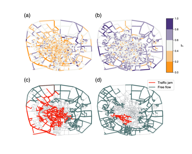
Figure 2: Traffic status of Chengdu road network. (a, b) Chengdu road networks denoted link weight as $r$ at (a) 08:00 and (b) 22:00 (Mon, June 15th, 2015). Roads that are closer to the orange indicate poor road conditions, while roads closer to the purple represent good road conditions. (c, d) The GCC of traffic jam (red edges) and free flow (green edges) when $p^{\rm(jam)}=0.3$ and $p^{\rm(free)}=0.3$, respectively, at (c) 8:00 and (d) 22:00 on the same day. The GCC of the traffic jam is formed near the center of the city, whereas that of the free flows occurs near highways outside the city.

We exploit the road network and taxi traffic data of Chengdu, China as a representative case study [26]. Chengdu, with a population of around 16.33 million, is a suitable urban area for traffic-related research due to its metropolitan nature. The city has a central downtown area surrounded by a ring-shaped arrangement of highways. The Chengdu road network comprises $N$ nodes (intersections) and $L$ directed links (roads) with $N=1902$ and $L=5943$. To evaluate the traffic conditions of each road, we use processed taxi data from approximately 12,000 taxis. This taxi dataset includes information on the time and speed at which taxis moved on each road segment, and it covers a 45-day period from June 1 to July 15 in the year 2015. To mitigate noise caused by traffic signals or minor traffic events, we average taxi speed $v$ over one-hour intervals on a road.

The Chengdu road network with the rescaled speed is depicted in Figs. 2(a) and 2(b). The spatial visualization of rescaled speed gives an overview of how well performing roads (purple links) and poorly performing roads (orange links) are distributed during both rush hour (8:00) and non-rush hour (22:00) periods. The original taxi data contains the partial time stamps as listed in Table 2, thus obtaining ten points of the rescaled average speed $r$ of every road segment for a given day.

Table 2: Road network and taxi speed data were collected in Chengdu, China [26]. The taxi speed data can be accessed for various time windows as provided by the empirical data. The embedded road structure remains static.

Period	Weekday or Weekend	Time Windows (hour)	$N$	$L$
June 1, 2015 to July 15, 2015	32 weekdays 13 weekend days (total 45 days)	03, 04, 08, 09, 12, 13, 17, 18, 21, 22	1902	5943

3 Analysis on the traffic clusters

3.1 Giant connected components of traffic jam and free flow

In network theory, a giant connected component can be understood as the main functional or robustness unit of a system, so we explore the formation behavior of the GCCs between two percolation processes according to the process in Fig. 1: link occupation in ascending order (traffic jam) and descending order (free flow) of the link weight $r$. In Figs. 2(c) and 2(d), we first depict the spatial patterns of the GCC at the same value of the occupation link density $p=0.3$ for rush hour (08:00) and non-rush hour (22:00). More explicitly, the occupation density in ascending and descending order is denoted by $p^{\rm(jam)}$ and $p^{\rm(free)}$, respectively. Despite the same number of occupied links (the same fraction $p$), the GCCs that will be defined soon have different spatial structural properties, for example, sizes and shapes, by times and percolation scenarios. As illustrated in Fig. 2(c), during the rush hour, the traffic-jam component is extensively distributed across the urban center and extends to some peripheral roads, as contrasted with the free-flow component formed along with the boundary only. When the traffic gets relatively smooth at night, the traffic-jam component emerges, confined to a much smaller area around the urban center [Fig. 2(d)]. Meanwhile, the free-flow component still occupies primarily the roads on the outskirts of the city, with a larger size than the traffic jam case.

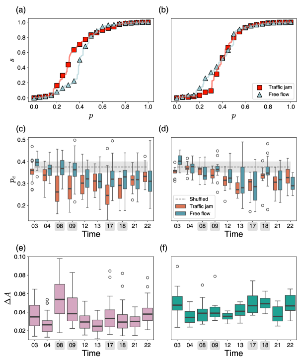
Figure 3: The growth behavior of the GCC for traffic jam and free flow. Snapshots of the relative size $s$ of the GCC versus the occupation fraction (link density) $p$ (a) at 8:00 (morning rush hour) on Monday, June 15th, 2015 and (b) at 22:00 (non-rush hour) on the same day. The $s^{\rm(jam)}$ and $s^{\rm(free)}$ at 22:00 behave similarly. The plot for the threshold point $p_{c}$ versus time $t$ (c) for weekdays and (d) for weekends. The transition points $p_{c}^{\rm(jam)}$ and $p_{c}^{\rm(free)}$ are represented by the orange box and blue box, respectively, and the dashed line indicates the threshold point on the weight-shuffled network, at $p_{c}^{\rm(shfl)}\simeq 0.376$. The plot for the gap area $\Delta A$ versus time $t$ (e) for weekdays and (f) weekends. The panels (c-f) display the quartile plot with the lower quartile $Q1$, the median or second quartile $Q2$, and the upper quartile $Q3$. The plot is a way to show the distribution of $p_{c}$ for (c), (e) 32 weekdays and (d), (f) 13 weekend days. The vertical length of the box stands for the interquartile range (IQR), $Q3-Q1$, the thick black line in a box indicates the median or the second quartile ($Q2$), and the whisker means the range between $Q1-1.5IQR$ and $Q3+1.5IQR$. Open circles out of the whisker correspond to the outliers. The gray box in the time axis is just for distinguishing two consecutive alternating time slots.

Figures 3(a) and 3(b) illustrate the behavior of the relative size $s$ of the GCC as a function of $p$, that is,

$$s(p;t)\equiv\frac{S_{1}(p;t)}{N},$$ (1)

for the representative cases on the same day as Fig. 2. The $S_{1}(p;t)$ is the number of nodes (intersections) belonging to the GCC at the occupation fraction $p$ for a given time $t$. For rush hour (8:00), $s^{\rm(jam)}$ and $s^{\rm(free)}$ behave differently. The GCC of the jamming cluster emerges at earlier $p$ than for the free flow cluster, and the $s^{\rm(jam)}$ increases with a steeper slope near the onset point of the giant component [Fig. 3(a)]. For the non-rush hour (22:00), the behaviors of $s^{\rm(jam)}$ and $s^{\rm(free)}$ are slightly different but the free-flow cluster still undergoes the same phenomena as the jamming cluster in the rush hour [Fig. 3(b)]. Either the dominant traffic situation of a traffic jam or smooth traffic manifests in the form of an earlier onset and rapid growth of the GCC, in terms of percolation. All individual growth patterns of the GCCs for 45 days at a given time are plotted in Fig. S1 in Supplemental Material.

As one of the indicators to describe the traffic situation, we examine the temporal behavior of the threshold $p_{c}$ at which the GCC emerges. The threshold fraction $p_{c}$ is evaluated with the help of both the giant and the second largest components which is a standard way to detect the threshold point in percolation theory (see Fig. S2 in Supplemental Materials for the detail). Considering the people’s different daily patterns, we analyze the patterns separately into weekdays and weekends. To verify the significance of the observed threshold values, we compare them with $p_{c}^{\rm(shfl)}\simeq 0.376$ numerically obtained by performing the traffic-jam and free-flow percolations in weight-shuffled networks (resulting in the absence of correlation) for a given road structure, which is trivially the same in both percolation scenarios. In Figs. 3(c) and 3(d), at first glance, one sees that the relations $p_{c}^{\mathrm{(jam)}}\lesssim p_{c}^{\rm(shfl)}$ and $p_{c}^{\mathrm{(free)}}\lesssim p_{c}^{\rm(shfl)}$ hold in most cases, which signals that the traffic correlation promotes the earlier onset of traffic clusters than expected.

Let us consider the median $\bar{p}_{c}$ (denoted by a thick gray line in the quartile plot) as a representative value of $p_{c}$. On weekdays, $\bar{p}_{c}^{\mathrm{(jam)}}$ and $\bar{p}_{c}^{\mathrm{(free)}}$ seem to behave in the opposite fashion with $\bar{p}_{c}^{\mathrm{(jam)}}<\bar{p}_{c}^{\mathrm{(free)}}$ kept. It implies that heavy-traffic roads are spatially clustered and then easily form the connected component of the congestion. The small $p_{c}^{\rm(jam)}$ during rush hour coincides with the previous observation in Beijing [19, 21], and we clarify this traffic situation more clearly by showing the large difference $\bar{p}_{c}^{\rm(jam)}$ from $\bar{p}_{c}^{\rm(free)}$. In addition, the opposite behavior of $\bar{p}$ on weekdays in Fig. 3(c) supports both the easy and relatively hard formations of congestion and free-flow clusters, respectively. On the other hand, similar trends in $\bar{p}_{c}$ on weekends could suggest that GCC formation occurs with similar ease in both traffic jams and free flow [Fig. 3(d)].

The respective temporal behaviors of the threshold values also provide insight into the traffic conditions. There are dips in $\bar{p}_{c}^{\mathrm{(jam)}}$ during the morning and evening rush hours on weekdays [Fig. 3(c)]. The two dips in Fig. 3(c) indicate that rush hour or non-rush hour strongly affects the formation of the congestion component, as already revealed in the previous study [21]. Otherwise, the rush/non-rush hour does not seem indispensable for the free-flow component supported by a slight increase at those times in Fig. 3(c). Rather, the fact that the high $\bar{p}_{c}^{\rm(free)}$ in the morning and the low in the evening means that the smooth roads are clustered differently depending on the forenoon or afternoon. The different temporal patterns of $\bar{p}_{c}^{\rm(jam)}$ and $\bar{p}_{c}^{\rm(free)}$ connote different conglomerate formation processes and smooth traffic. On weekends, people’s activities are more likely concentrated around noon and late at night, rather than during typical commute times (around 8:00 and 17:00). This may result in low values of $\bar{p}$ at different times from weekdays, such as around 13:00 and 21:00.

The GCC growth pattern can be characterized by its point of onset and growth rate, and the small $p_{c}$ only ensures the early onset. The growth steepness can be evaluated by the critical exponent of the order parameter $s$ in percolation theory, but the exponent is neither analytically nor numerically ill-defined in these empirical data due to inherent fluctuation. To understand the entire behavior including the growth rate near the transition point, we measure the absolute areal difference or the gap area $\Delta A$ between two curves $s^{\rm(jam)}(p)$ and $s^{\rm(free)}(p)$ as

$$\Delta A\equiv\int_{0}^{1}\left|s^{\mathrm{(jam)}}(p)-s^{\mathrm{(free)}}(p)\right|\mathop{}\!\mathrm{d}p.$$ (2)

The gap area $\Delta A$ captures how much the two curves differ, rather than which curve is dominant, and is bounded from 0 to 1. When the two curves are perfectly the same as each other, $\Delta A=0$. The maximum difference $\Delta A=1$ corresponds to the case that $s(p_{c})=1$ at $p_{c}=1$ in one curve and $s(p_{c})=1$ at $p_{c}=0$ in the other curve.

For all days and times, the gap area is small but not zero, and its median value stays around 0.03 as seen in Figs. 3(e) and  3(f). Meantime, one can observe the large value of the median $\overline{\Delta A}\approx 0.05$ at the morning rush hour (8:00) on weekdays. Taking into account the growth pattern of $s$ with increasing concave-down shape (Fig. S1) as well as $\bar{p}_{c}^{\rm(jam)}<\bar{p}_{c}^{\rm(free)}$ at that time, we suspect that the quite long-lasting relation of $s^{\rm(jam)}>s^{\rm(free)}$ over all ranges of $p$ rather than $s^{\rm(jam)}<s^{\rm(free)}$ contributes to large $\Delta A$.

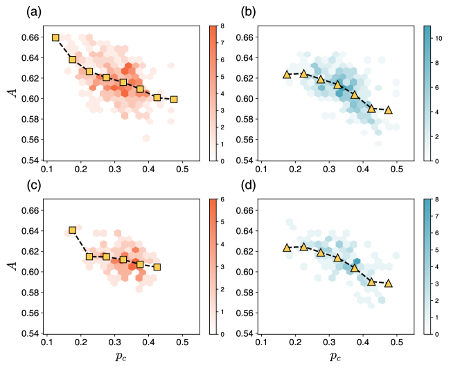
Figure 4: Density plots of the area $A$ under the curve versus threshold fraction $p_{c}$ on (a), (b) weekdays and (c), (d) weekends. The left panels (a), (c) and the right ones (b), (d) indicate the cases of traffic-jam percolation and free-flow percolation, respectively. The yellow squares and triangles represent the average values at a $p_{c}$. Overall, $A$ and $p_{c}$ are negatively correlated, with the Pearson correlation coefficients (a) $-0.49$, (b) $-0.63$, (c) $-0.36$, and (d) $-0.63$, respectively.

In most cases, $s$ increases trivially in such a way as to cause rapid growth after $p_{c}$ and then slow saturation at large $p$. That is, early $p_{c}$ can guarantee fast arrival at $s\approx 1$, and there is no nontrivial growth pattern such as a long plateau at a low $s$ after early $p_{c}$ and then a super rapid jump to $s=1$ at high $p$. This entire growth pattern can be characterized by the threshold fraction $p_{c}$ versus the area under the curve $A$ as

$$A\equiv\int_{0}^{1}{s(p)\mathop{}\!\mathrm{d}p}.$$ (3)

The area $A$ can assess the extent of the GCC’s growth, and the curve $s(p)$ with $A$ closer to 1 might be highly likely to be increasing concave-down and have a large slope near the $p_{c}$. The expected trivial curve shape gives the high $A$ with the small $p_{c}$ whereas the exemplified nontrivial curve gives the small $A$ at small $p_{c}$. As shown in Fig. 4, throughout weekdays/weekends and traffic-jam/free-flow, the $A$ and $p_{c}$ show significantly negative correlations, which means the trivial growth patterns of $s$ prevail significantly. This correlation supports the long-lasting relation $s^{\rm(jam)}>s^{\rm(free)}$ at the morning rush hour.

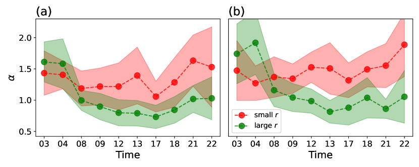
Figure S3: The behavior of the difference between $p_{c}^{\mathrm{(jam)}}$ and $p_{c}^{\mathrm{(free)}}$. (a, b) The temporal change of the difference between $p_{c}^{\mathrm{(jam)}}$ and $p_{c}^{\mathrm{(free)}}$ on (a) weekdays and (b) weekends. The larger the magnitude of $p_{c}^{\mathrm{(jam)}}-p_{c}^{\mathrm{(free)}}$ is with a plus (minus) sign, the more likely the free-flow (traffic jam) GCC will occur. The difference can aid in figuring out traffic situations. (c) Then the scatter plot about $p_{c}^{\mathrm{(jam)}}-p_{c}^{\mathrm{(free)}}$ versus $\Delta A$. The Pearson correlation coefficient is estimated separately for $p_{c}^{\mathrm{(jam)}}-p_{c}^{\mathrm{(free)}}<0$ (brown) and $p_{c}^{\mathrm{(jam)}}-p_{c}^{\mathrm{(free)}}>0$ (green), as -0.61 and 0.44, respectively. Whether congestion or free flow is dominant, the gap area $\Delta A$ increases significantly as the degree of dominance grows.

The difference between $p_{c}^{\rm(jam)}$ and $p_{c}^{\rm(free)}$ seems to be usually dedicated to the $\Delta A$, but the gap area $\Delta A$ at evening rush hour 17:00 on weekdays is similar to those of the non-rush hours, despite the difference of threshold points as large as the morning rush hour. From these observations, we conjecture that the traffic-jam cluster is more easily formed than the free-flow cluster (supported by $p_{c}^{\rm(jam)}<p_{c}^{\rm(free)}$) and that the $s^{\rm(jam)}$ at the evening rush hour after the onset grows not so rapidly as $s^{\rm(jam)}$ at the morning rush hour, which leads to small $\Delta A$ compared with the morning. Any single indicator alone, either of $p_{c}$ and $\Delta A$, is hard to perfectly explain the traffic situation, which is natural because the complex system is not simple. Instead, the two measurements play complementary roles in more thoroughly understanding the simultaneous behaviors of traffic congestion and free-flow components. The effect of the difference itself as $p_{c}^{\rm(jam)}-p_{c}^{\rm(free)}$ is displayed in Fig. S3 in Supplemental Materials.

3.2 Correlation analysis in the context of urban transportation

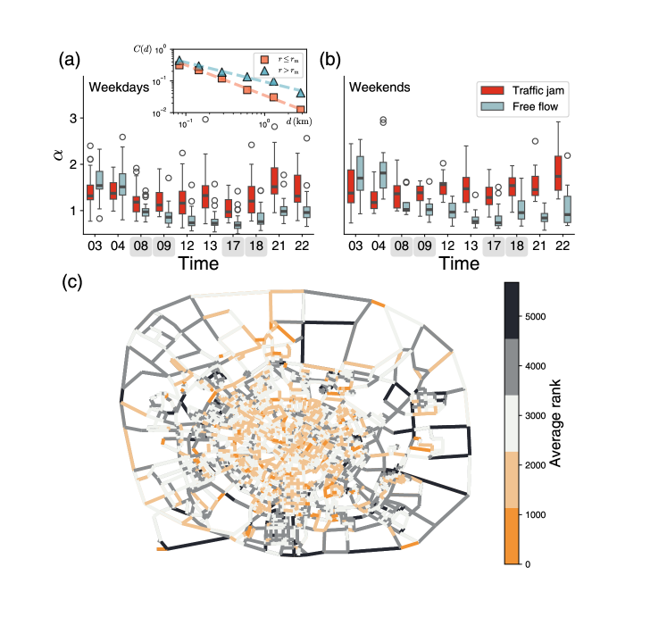
Figure 5: The exponent $\alpha$ represents the long-rangeness of weight-weight correlation as time for (a) weekdays and (b) weekends. The orange quartile box plot represents the results where $r\leq r_{\mathrm{m}}$ and the blue one represents the results where $r>r_{\mathrm{m}}$. (a) Inset: Weight-weight correlation as a function of the distance between two roads on June 4th, 2015, 17:00. The correlation of roads where $r\leq r_{\mathrm{m}}$ is represented with orange square, and the orange dashed line indicates the power-law fit. The blue triangle and dashed line are depicted as the correlation and power-law fitting line of roads where $r>r_{\mathrm{m}}$ An exponent of the power-law of $r\leq r_{\mathrm{m}}$ is 0.96 and the one of $r>r_{\mathrm{m}}$ is 0.61. (c) Chengdu road network is depicted by the average rank of percolation occupation order for traffic-jam percolation. The roads that are closer to yellow are the ones occupied first in traffic-jam percolation, while the roads closer to black are the ones occupied first in free-flow percolation. In the case of traffic-jam percolation, the roads in the center of the city are preferentially occupied. In contrast, in the case of free-flow percolation, the roads on the outskirts of the city are occupied first.

The traffic-jam and free-flow components emerge at different occupation fractions $p$, and their growth patterns differ. This variation in the formation patterns may be due to correlation; the closer the roads with small (large) $r$ are to each other, the more easily the GCC of the traffic jam (free flow) can form. This hypothesis can be supported by both $p_{c}^{\rm(jam)}$ and $p_{c}^{\rm(free)}$ smaller than $p_{c}^{\rm(shfl)}$ for most cases in Figs. 3(c) and 3(d). This seems to agree with the previous finding that the spatial positive (negative) correlation promotes the earlier (later) emergence of the GCC than the uncorrelated structure in a two-dimensional space [23]. Thus, we explore the correlation of traffic flows and extend our discussion.

We examine the correlation $C(d)$ of the traffic flow, that is, the weight-weight correlation, for the distance $d$ calculated as

$$C(d;t)=\frac{\sum_{ij}\big{(}r_{i}-\langle r\rangle\big{)}\big{(}r_{j}-\langle r\rangle\big{)}\delta(d_{ij}-d)}{\sqrt{\sum_{ij}\left[\big{(}r_{i}-\langle r\rangle\big{)}\big{(}r_{j}-\langle r\rangle\big{)}\right]^{2}\delta(d_{ij}-d)}},$$ (4)

where $d_{ij}$ is the geodesic distance, measured in integer binning, between roads $e_{i}$ and $e_{j}$, and $\langle r\rangle=\sum_{i}r_{i}(t)/L$. Assuming a power-law form of the correlation as $C(d)\sim d^{-\alpha}$, the small and large values of the exponent $\alpha$ imply the presence of the long-range and short-range correlation, respectively, which we call the “long-rangeness”.

The case of $0<\alpha<2$ ($\alpha>2$) corresponds to the positive (negative) correlation, respectively, and the case of $\alpha=2$ stands for no correlation as compared to the previous study [23]. To estimate the long-rangeness exponent $\alpha$ for the traffic jam and free flow, we compute the correlation in Eq. (4) separately into two groups $r\leq r_{m}$ and $r>r_{m}$ with $r_{m}$ being the median of the rescaled speed from a distribution for a given day. We suppose that roads with $r\leq r_{m}$ ($r>r_{m}$) can serve as clusters of traffic jams (free flow). As an example, $C(d)$ as a function of $d$ at 17:00 (the evening rush hour) on June 4, 2015, is shown in the inset of Fig. 5(a), following the power law with exponents less than 2. In most cases, the exponent $\alpha$ is estimated as $\alpha\lesssim 2$ on weekdays and weekends as shown in Figs. 5(a) and 5(b), respectively, and then tend to decrease in the daytime and increase in the nighttime (see Supplemental Materials for Fig. S4).

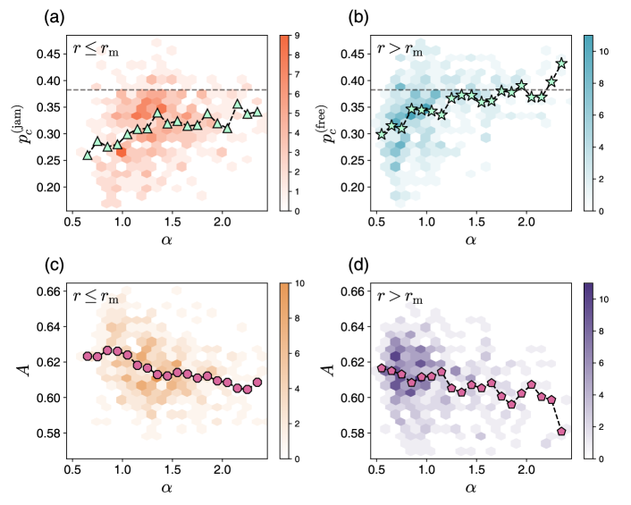
Figure 6: The relation of the long-rangeness exponent $\alpha$ with (a), (b) the threshold fraction $p_{c}$ and with (c), (d) the area $A$ under the curve, for the cases of (a), (c) $r\leq r_{\mathrm{m}}$ and (b), (d) $r>r_{\mathrm{m}}$. The hexagonal tiles are the density plots, and other green and purple symbols with interpolation lines are average values at $\alpha$. In the upper panels (a) and (b), a dashed line represents $p_{c}^{\rm(*)}$ of random percolation on the Chengdu road network.

In contrast with the observed results, one may expect the lower $\alpha$ for the case of $r\leq r_{m}$ than $r>r_{m}$ in the example of the rush hour, owing to the early formation of the congesting cluster, i.e., smaller $p_{c}^{\rm(jam)}$. We need to emphasize again that the traffic-smoothing roads are usually distributed outwards from the city center and most of the outskirt roads have long lengths [Figs. 2(c) and 2(d)], resulting in the inherently longer-range correlation within the collection of smoothing roads than the congested roads mainly emerging in the central area. Most of the traditional urban city is known to have a spatial center-periphery structure [28, 29]; the center area is a web-like structure with denser connections, while the roads in the periphery are less connected to each other but more connected to the center. To confirm the spatial structure of the traffic cluster, we assign the average rank of the occupation in ascending order to each road over the entire time course [Fig. 5(c)]. The low (high) average rank connotes the occupation priority in the traffic-jam (free-flow) percolation. As expected, the low-ranked (congested) roads are concentrated in the urban center mainly consisting of short roads. The high-ranked (smooth) roads are distributed in the vicinity of the urban boundaries consisting of long roads. Due to inherent features, we need to interpret the role of the exponent $\alpha$ separately for the traffic jam and the free flow, when introducing the real length.

The previous study has revealed the relationship between the critical point and an exponent that describes the extent of the long-range correlation, i.e., the decreasing behavior of the exponent as a function of the critical point [23]. In terms of the exponent $\alpha$ defined in a way opposite to the previous study, this should turn out to be an increasing behavior, and we observe this pattern as seen in Figs. 6(a) and 6(b). These observations allow us to guess the responsibility of the correlation for the early onset of the traffic clusters, although a rigorous theoretical approach is unlikely to be applied. The higher $p_{c}^{\rm(free)}$ than $p_{c}^{\rm(jam)}$ on average at the similar value of $\alpha$ may be caused by the network detail near the urban periphery and center. How do we interpret the relation between the exponent $\alpha$ and the threshold point $p_{c}$ phenomenologically? Let us take an example of traffic congestion. If one road is stuck, the adjacent roads could get stuck sequentially, and it goes on and on. Similar speeds spread across the road network from the seed road, such as in the contact process. The stronger correlation (small $\alpha$) precipitates a greater spread of similar traffic status than expected, naturally leading to easy formation of the traffic component (small $p_{c}$).

The long-range correlation can promote the growth of the giant component, as well as its early onset. We used the area $A$ under the curve again in Eq. (3). The area under the curve $A$ as a function of the long-rangeness exponent $\alpha$ is shown in Figs. 6(c) and 6(d), and $A$ is in the range of 0.56 to 0.67 in both cases of $r<r_{m}$ and $r>r_{m}$, which is quite large considering the small contribution of $\int_{0}^{p_{c}}{s\,dp}$. The decreasing behavior of $A$ as to $\alpha$ can assist our hypothesis that long-range correlation (small $\alpha$) induces the rapid growth of the giant component (large $A$) in general. The Pearson correlation coefficient is evaluated as $-0.32$ for $r\leq r_{m}$ and as $-0.22$ for $r>r_{m}$. The relations among small $p_{c}$, large $A$, and small $\alpha$ shown in Figs. 4 and 6 coincide with each other and give us a lesson: the correlation induces the early onset of the traffic cluster at a rapid growth rate, which brings us to observe a dominant traffic situation, traffic-jam or free-flow state.

4 Conclusions

As cities develop, urban transportation becomes increasingly complex. The variety and number of transportation services are growing, making it challenging to evaluate transportation phenomena using a single metric. For example, a city with significant traffic jams may recover quickly, while a city with generally smooth traffic flow may be vulnerable to minor congestion. Therefore, evaluating urban transportation, a complex system, requires comparing multiple indicators. Unlike previous research that focused solely on traffic jams or free-flow phenomena, our study simultaneously observes both traffic processes within the urban road network. We identify traffic jam (free flow) clusters by marking roads with bad (good) traffic conditions (Fig. 1). Traffic jam clusters form remarkably easily during rush hours, as the small $p_{c}$ indicates. This finding is consistent with previous studies, but our approach allows us to assess how easily and quickly congestion emerges through a comparison with $p_{c}$ of free-flow percolation. This is further clarified by the large value of the gap area $\Delta A$ during rush hour. Neither $p_{c}$ nor $\Delta A$ alone perfectly describes the consistent trends, but together they play a synergistic and complementary role in understanding traffic patterns (Fig. 3). Considering both traffic congestion and free flow using the two quantities $p_{c}$ and $\Delta A$ enriches the analysis of the urban transportation system. Additionally, we explored the weight-weight correlation and found that stronger correlations may drive the dominant traffic phenomenon (Figs. 5 and 6). These insights help to pinpoint specific areas for intervention to maintain the sustainability and safety of traffic flow.

Our method and findings offer practical applications to improve the reliability and safety of urban road networks. For example, percolation analysis can dynamically optimize traffic signal timings based on real-time conditions, reducing congestion and accidents. Emergency response systems can benefit from routing through less congested paths, ensuring faster response times. Urban planners can apply our insights to prioritize infrastructure development in critical, congestion-prone areas. Implementing congestion pricing and improving public transportation on high-risk routes can further alleviate traffic issues. Real-time traffic management systems can distribute vehicles more evenly, while predictive maintenance can keep roads in better condition, preventing congestion-related damage. Additionally, smart parking solutions can direct drivers to available spots in less congested locations, reducing unnecessary driving and enhancing overall traffic flow. These applications demonstrate the significant impact of our research on developing effective traffic management strategies and improving urban road safety in the near future.

While this study focused on the case of Chengdu, our approach can be extended to other cities given sufficient data. Chengdu’s road structure resembles a core-peripheral ring pattern, whereas some planned cities exhibit a more lattice-like structure. In a previous study [28], we revealed how road structure affects traveling patterns. Similarly, the road network topology could influence traffic percolation behavior and system resilience [30]. Beyond empirical investigations, a theoretical modeling approach can further enhance our understanding of traffic dynamics. Introducing traffic simulations on networked structures would allow us to control various conditions. Designing correlated percolation models to mimic traffic situations is an essential next step, which we leave for future work.

5 Acknowledgments

This work was supported by the National Research Foundation (NRF) of Korea through Grant Numbers. NRF-2023R1A2C1007523 (S.-W.S.), RS-2024-00341317 (M.J.L.) and NRF-2022R1A5A7033499 (M.L.). This work was also partly supported by the Institute of Information & communications Technology Planning & Evaluation (IITP) grant funded by the Korean government (MSIT) (No.RS-2022-00155885, Artificial Intelligence Convergence Innovation Human Resources Development (Hanyang University ERICA)). We also acknowledge the hospitality at APCTP where part of this work was done.

6 Supplemental Material

Appendix Note 1 Growth of traffic GCCs as the occupation fraction $p$

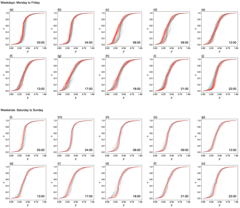
Figure S1: The relative size of the GCC, $s_{G}$, versus occupation fraction $p$ for (a-j) 32 weekdays, (l-u) 13 weekends at a given time. Each panel corresponds to a given time slot, and the traffic-jam and free-flow GCCs are represented by red and blue lines, respectively.

We obtain the relative size of the giant connected component curve as a function of the occupation fraction, which results in (two types of percolation)$\times(32\mathrm{\,weekdays\,or\,}13\mathrm{\,weekends})\times(\mathrm{ten\,time-slots})$ curves $s_{G}(p)$ for our analysis. Every single curve is plotted in Fig. S1. At a glance, almost all curves appear as increasing concave-down shapes. In shape, an early $p_{c}$ can ensure the early growth of $s$, resulting in a large area under the curve [Fig. 4 in the main text].

Appendix Note 2 Specifying percolation threshold $p_{c}$

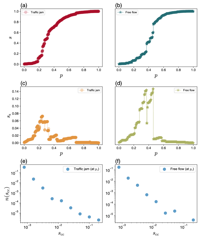
Figure S2: Results of (a, c, e) traffic-jam and (b, d, f) free-flow percolations on June 4, 2015, 08:00. The relative size $s$ of the GCC of (a) traffic jam and (b) free flow behaves with increasing concave-down form. (c, d) The relative size $s_{\mathrm{s}}$ of the SGCC can have multiple peaks. (e, f) The cluster size distribution $n(s_{\mathrm{cc}})$ at $p_{c}$ follows a power-law form.

In percolation theory, the critical point $p_{c}$ is the phase transition point where the size of the GCC emerges, scaling with the size of the system. At this moment, various scale-invariant phenomena are observed, e.g., the divergence of the second giant connected component (SGCC) with a power-law form. This scale-invariant divergence cannot be obtained in a finite system, so the peak position (instead of the divergence point) of the SGCC has helped to measure $p_{c}$. However, in real-world data, multiple peaks of the SGCC exist due to their unavoidable innate fluctuations as well as finiteness, making it challenging to define only one $p$ that gives a significant single peak of SGCC as shown in Fig. S2. Let us denote $s$ and $s_{s}$ as the relative sizes of the GCC and SGCC, respectively. In the traffic-jam case, it can be said that there is only one large peak of $s_{s}$, but two peaks having similar $s_{s}$ seem to exist in the free-flow case. Which of the two peaks will give the threshold points?

This observation drives us to define the threshold point in a more practical way confined to our traffic data. We impose the criteria in such a way that

$$p_{c}\equiv\arg\max_{p}s_{s}(p)\text{ only\,if }s(p)\leq 0.5.$$ (1)

The condition $s\leq 0.5$ is for ensuring that the GCC is not already significant when the $s_{s}$ peaks and resolves the vagueness like the abovementioned case in Fig. S2(d). Without this restriction, the pure maximum $s_{s}$ emerges at $p=0.458$. This $p$ gives the quite large value $s\approx 0.8$, and this large $s$ close to 1 does not describe the vicinity of the transition point. With the restriction $s\leq 0.5$ imposed, the first peak of $s_{s}$ at $p=0.370$ gives $s\approx 0.4$, which sounds more reasonable.

At the critical point, the cluster size distribution $n(s)$ follows the power-law form. We investigate the distribution $n(s)$ at the $p_{c}$ in Eq. (1). The distribution displayed in Figs. S2(e) and S2(f) follows a power-law form as expected.

Figure S4: Temporal behavior of the long-rangeness exponent $\alpha$ on (a) weekdays and (b) weekends. The small $r$ means $r\leq r_{\mathrm{m}}$ while the large $r$ means $r>r_{\mathrm{m}}$ with $r_{m}$ being the median. $\alpha$ for the large-$r$ case is lower than that for the small-$r$ case, on average. $\alpha$ for the small-$r$ case seems to decrease during rush hours on weekdays. The exponent for the large-$r$ case decreases until the evening rush hour. On weekends, the $\alpha$ of small $r$ increases after evening rush hour. The $\alpha$ of large $r$ seems to behave like the case of the weekdays.

References

- Wang et al. [2012] Pu Wang, Timothy Hunter, Alexandre M. Bayen, Katja Schechtner, and Marta C. González. Understanding road usage patterns in urban areas. Scientific reports, 2(1):1001, 2012.
- Hamedmoghadam et al. [2021] Homayoun Hamedmoghadam, Mahdi Jalili, Hai L Vu, and Lewi Stone. Percolation of heterogeneous flows uncovers the bottlenecks of infrastructure networks. Nature communications, 12(1):1254, 2021.
- Kim [2016] Byeongsun Kim. Exploring emergency areas for medical service using microscopic traffic simulation model. Spatial Information Research, 24:75–84, 2016.
- Sarkar et al. [2021] Trishna Sarkar, Debabrata Sarkar, and Prolay Mondal. Road network accessibility analysis using graph theory and gis technology: a study of the villages of english bazar block, india. Spatial Information Research, 29(3):405–415, 2021.
- Wen et al. [2024] Huiying Wen, Yichen Ye, and Lin Zhang. Optimizing road networks in underdeveloped regions for improving comprehensive efficiency integrated by accessibility, vulnerability and socioeconomic interaction. Reliability Engineering & System Safety, 243:109848, 2024.
- Kwon et al. [2023] Yungi Kwon, Jung-Hoon Jung, and Young-Ho Eom. Global efficiency and network structure of urban traffic flows: A percolation-based empirical analysis. Chaos: An Interdisciplinary Journal of Nonlinear Science, 33(11), 2023.
- Serok et al. [2023] Nimrod Serok, Shlomo Havlin, and Efrat Blumenfeld Lieberthal. Enhancing traffic flow efficiency through an innovative decentralized traffic control based on traffic bottlenecks, 2023.
- Chowdhury et al. [2000] Debashish Chowdhury, Ludger Santen, and Andreas Schadschneider. Statistical physics of vehicular traffic and some related systems. Physics Reports, 329(4-6):199–329, 2000.
- Lee and Kim [2011] Hyun Keun Lee and Beom Jun Kim. Dissolution of traffic jam via additional local interactions. Physica A: Statistical Mechanics and its Applications, 390(23):4555–4561, 2011. ISSN 0378-4371.
- Boccaletti et al. [2006] S. Boccaletti, V. Latora, Y. Moreno, M. Chavez, and D.-U. Hwang. Complex networks: Structure and dynamics. Physics Reports, 424(4):175–308, 2006. ISSN 0370-1573.
- Ganin et al. [2017] Alexander A Ganin, Maksim Kitsak, Dayton Marchese, Jeffrey M Keisler, Thomas Seager, and Igor Linkov. Resilience and efficiency in transportation networks. Science advances, 3(12):e1701079, 2017.
- Saberi et al. [2020] Meead Saberi, Homayoun Hamedmoghadam, Mudabber Ashfaq, Seyed Amir Hosseini, Ziyuan Gu, Sajjad Shafiei, Divya J Nair, Vinayak Dixit, Lauren Gardner, S Travis Waller, et al. A simple contagion process describes spreading of traffic jams in urban networks. Nature communications, 11(1):1616, 2020.
- Jung and Eom [2023] Jung-Hoon Jung and Young-Ho Eom. Empirical analysis of congestion spreading in seoul traffic network. Physical Review E, 108(5):054312, 2023.
- Helbing [2001] Dirk Helbing. Traffic and related self-driven many-particle systems. Reviews of modern physics, 73(4):1067, 2001.
- Daqing et al. [2014] Li Daqing, Jiang Yinan, Kang Rui, and Shlomo Havlin. Spatial correlation analysis of cascading failures: congestions and blackouts. Scientific reports, 4(1):5381, 2014.
- Wang et al. [2015] Feilong Wang, Daqing Li, Xiaoyun Xu, Ruoqian Wu, and Shlomo Havlin. Percolation properties in a traffic model. Europhysics Letters, 112(3):38001, 2015.
- Petri et al. [2013] Giovanni Petri, Paul Expert, Henrik J Jensen, and John W Polak. Entangled communities and spatial synchronization lead to criticality in urban traffic. Scientific reports, 3(1):1798, 2013.
- Ambühl et al. [2023] Lukas Ambühl, Monica Menendez, and Marta C González. Understanding congestion propagation by combining percolation theory with the macroscopic fundamental diagram. Communications Physics, 6(1):26, 2023.
- Li et al. [2015a] Daqing Li, Bowen Fu, Yunpeng Wang, Guangquan Lu, Yehiel Berezin, H Eugene Stanley, and Shlomo Havlin. Percolation transition in dynamical traffic network with evolving critical bottlenecks. Proceedings of the National Academy of Sciences, 112(3):669–672, 2015a.
- Zhang et al. [2019] Limiao Zhang, Guanwen Zeng, Daqing Li, Hai-Jun Huang, H Eugene Stanley, and Shlomo Havlin. Scale-free resilience of real traffic jams. Proceedings of the National Academy of Sciences, 116(18):8673–8678, 2019.
- Zeng et al. [2019] Guanwen Zeng, Daqing Li, Shengmin Guo, Liang Gao, Ziyou Gao, H Eugene Stanley, and Shlomo Havlin. Switch between critical percolation modes in city traffic dynamics. Proceedings of the National Academy of Sciences, 116(1):23–28, 2019.
- Zeng et al. [2020] Guanwen Zeng, Jianxi Gao, Louis Shekhtman, Shengmin Guo, Weifeng Lv, Jianjun Wu, Hao Liu, Orr Levy, Daqing Li, Ziyou Gao, et al. Multiple metastable network states in urban traffic. Proceedings of the National Academy of Sciences, 117(30):17528–17534, 2020.
- Prakash et al. [1992] Sona Prakash, Shlomo Havlin, Moshe Schwartz, and H Eugene Stanley. Structural and dynamical properties of long-range correlated percolation. Physical Review A, 46(4):R1724, 1992.
- Taillanter and Barthelemy [2021] Erwan Taillanter and Marc Barthelemy. Empirical evidence for a jamming transition in urban traffic. Journal of the Royal Society Interface, 18(182):20210391, 2021.
- Li et al. [2021] Ming Li, Run-Ran Liu, Linyuan Lü, Mao-Bin Hu, Shuqi Xu, and Yi-Cheng Zhang. Percolation on complex networks: Theory and application. Physics Reports, 907:1–68, 2021. ISSN 0370-1573. Percolation on complex networks: Theory and application.
- Guo et al. [2019] Feng Guo, Dongqing Zhang, Yucheng Dong, and Zhaoxia Guo. Urban link travel speed dataset from a megacity road network. Scientific data, 6(1):61, 2019.
- Li et al. [2015b] Daqing Li, Qiong Zhang, Enrico Zio, Shlomo Havlin, and Rui Kang. Network reliability analysis based on percolation theory. Reliability Engineering & System Safety, 142:556–562, 2015b. ISSN 0951-8320.
- Lee et al. [2023] Minjin Lee, SangHyun Cheon, Seung-Woo Son, Mi Jin Lee, and Sungmin Lee. Exploring the relationship between the spatial distribution of roads and universal pattern of travel-route efficiency in urban road networks. Chaos, Solitons & Fractals, 174:113770, 2023. ISSN 0960-0779.
- Levinson and El-Geneidy [2009] David Levinson and Ahmed El-Geneidy. The minimum circuity frontier and the journey to work. Regional science and urban economics, 39(6):732–738, 2009.
- Lu et al. [2024] Qing-Long Lu, Wenzhe Sun, Jiannan Dai, Jan-Dirk Schmöcker, and Constantinos Antoniou. Traffic resilience quantification based on macroscopic fundamental diagrams and analysis using topological attributes. Reliability Engineering & System Safety, 247:110095, 2024. ISSN 0951-8320.