Quantum Mpemba effects in many-body localization systems

Abstract

The nonequilibrium dynamics of quantum many-body systems have attracted growing attention due to various intriguing phenomena absent in equilibrium physics. One famous example is the quantum Mpemba effect, where the subsystem symmetry is restored faster under a symmetric quench from a more asymmetric initial state. The quantum Mpemba effect has been extensively studied in integrable and chaotic systems. In this Letter, we investigate symmetry restoration and quantum Mpemba effect in many-body localized systems with various initial states. We reveal that the symmetry can still be fully restored in many-body localization phases without approaching thermal equilibrium. Furthermore, we demonstrate that the presence of the quantum Mpemba effect is universal for any initial tilted product state, contrasting to the cases in the chaotic systems where the presence of the quantum Mpemba effect relies on the choice of initial states. We also provide a theoretical analysis of symmetry restoration and quantum Mpemba effects with the help of the effective model for many-body localization. This Letter not only sheds light on extending the quantum Mpemba effect to more non-equilibrium settings but also contributes to a deeper understanding of the many-body localization.

Introduction.— The nonequilibrium physics harbors various counterintuitive phenomena and has attracted increasing attention. One famous example is the Mpemba effect [1], namely, hot water freezes faster than cold water under identical conditions. This effect has been identified and investigated in various classical systems [2, 3, 4, 5, 6, 7, 8, 9, 10, 11, 12] and open quantum systems [13, 14, 15, 16, 17, 18, 19, 20, 21, 22, 23, 24, 25]. Recently, a quantum version of the Mpemba effect in isolated systems has been discussed [26] where the subsystem U(1) symmetry starting from a more asymmetric initial state can be restored faster than that from a more symmetric initial state under the quench of a symmetric Hamiltonian. This novel phenomenon is dubbed the quantum Mpemba effect (QME) and has been extensively investigated in integrable systems [27, 28, 29, 30, 31, 32], free dissipative systems [33, 34], chaotic systems [35, 36, 37], and trapped-ion experiments [38]. Besides, the QME has also been extended to the restoration of other symmetries, including the non-Abelian SU(2) symmetry [35] and the translation symmetry [39]. More importantly, the underlying mechanisms of QME in both integrable and chaotic systems have been established attributing to the distinct charge transport properties [31] and quantum thermalization speeds [35] associated with different initial states, respectively.

Many-body localization (MBL) phases [40, 41, 42, 43, 44] occur in one-dimensional isolated interacting systems in the presence of sufficiently strong disorders [45, 46] or quasiperiodic potentials [47]. In the MBL phase, the system violates the eigenstate thermalization hypothesis  [48, 49, 50, 51, 52] and exhibits various exotic behaviors, including the logarithmic spread of entanglement [53, 54, 55, 56, 57, 58, 59] and emergent local integrals of motion [60, 61]. The MBL Hamiltonian respects the U(1) symmetry, but the symmetry restoration and the QME in the quench under the MBL Hamiltonian have not been studied before. A natural question that arises is whether the U(1) symmetry can be restored in the MBL phase as the system fails to thermalize under MBL evolution. A companion further question is whether the QME exists in the MBL phase. More importantly, a theoretical understanding of the presence or absence of symmetry restoration and QME in the MBL phase is strongly required.

Table 1: Main results of symmetry restoration and QME in MBL and chaotic systems

Systems and initial states	Symmetry restoration	QME
MBL from any tilted product states &	finite-size symmetry	always present
chaotic system from tilted ferromagnetic states	broken crossover (see Fig. 3)
chaotic system from	fully restoration for any $\theta$ [62]	state-dependent [63]
other tilted product states

In this Letter, we investigate the U(1) symmetry restoration and the associated QME starting from various tilted product states in the thermal and MBL phases via adjusting the strength of disorder in the Hamiltonian. We find that the symmetry can be fully restored in the thermodynamic limit for both phases. In the thermal phase, the QME is present and absent for the tilted ferromagnetic state and tilted Néel state respectively, similar to that observed in U(1)-symmetric random circuits [35], which can be understood through the lens of quantum thermalization. In the MBL phase, the symmetry can also be fully restored, which presents a nontrivial example for the long-time evolved state that restores the symmetry but doesn’t reach thermal equilibrium. The associated symmetry restoration timescale is exponential in the system size. However, the emergence of the QME is universal in the MBL phase, independent of the initial tilted product state choices. These unexpected results in MBL systems indicate a distinct underlying mechanism as compared to integrable and chaotic systems.

To theoretically understand the mechanism behind symmetry restoration and QME in the MBL phase, we consider the corresponding effective model based on the emergent local integrals of motion [60, 61]. In the long time limit, the degrees of symmetry breaking can be analytically obtained. The results are the same for different initial tilted product states in MBL systems and are also consistent with the results from chaotic systems starting from initial tilted ferromagnetic states. However, the results in chaotic systems with other initial states show different patterns. Consequently, MBL quench from any tilted product states and chaotic quench from tilted ferromagnetic states share similar symmetry restoration behaviors including the presence of QME while QME might be absent in chaotic quench from other tilted product states. The main results are summarized in Table. 1. We also conduct a direct numerical simulation and observe the QME in the symmetry restoration dynamics under the quench of the MBL effective model.

Model and observables.— In this Letter, we consider the following one-dimensional interacting Aubry-André (AA) model [47, 64, 65, 66, 67, 68, 69, 70, 71, 72, 73] hosting the MBL transition,

$$H= - \sum_{i}(\sigma^{x}_{i}\sigma^{x}_{i+1}+\sigma^{y}_{i}\sigma^{y}_{i+1})+V\sum_{i}\sigma^{z}_{i}\sigma^{z}_{i+1}$$

$$+ \sum_{i}W_{i}\sigma^{z}_{i},$$

where $\sigma_{i}^{x,y,z}$ is the Pauli matrix at site $i$, $V$ is the strength of interaction and fixed to $\frac{1}{2}$ unless otherwise specified, $W_{i}=W\cos(2\pi\alpha i+\phi)$ is the quasiperiodic potential with strength $W$, $\alpha=\frac{\sqrt{5}+1}{2}$, and $\phi$ is the random phase to be averaged. We use the open boundary conditions throughout the work. There is a many-body localization transition from the thermal phase to the MBL phase in this model driven by the quasiperiodic potential strength $W$ with critical strength $W_{c}\approx 3.3$ . We have also investigated symmetry restoration and QME in the interacting model with random potentials [46, 45, 74], and the qualitative behaviors remain the same [62].

To quantify the degrees of symmetry breaking in subsystem $A$, we employ the entanglement asymmetry (EA) [26] which has been extensively studied as a symmetry broken measure in various physical contexts [75, 76, 77, 78, 79, 80, 81, 82]. This quantity is defined as

$$\Delta S_{A}=S(\rho_{A,Q})-S(\rho_{A}),$$ (2)

i.e., the difference of the von Neumann entropy between the reduced density matrix of subsystem $A$ chosen as the leftmost $N_{A}$ sites, $\rho_{A}$, and $\rho_{A,Q}=\sum_{q}\Pi_{q}\rho_{A}\Pi_{q}$ where $\Pi_{q}$ is the projector to the charge sector with $Q_{A}=\sum_{i\in A}\sigma_{i}^{z}=q$, namely, $\rho_{A,Q}$ only keeps the block diagonal elements of $\rho_{A}$. EA is non-negative by definition and only vanishes when $\rho_{A}$ is block diagonal for the subsystem charge sectors, i.e., the reduced density matrix $\rho_{A}$ is U(1) symmetric. Therefore, $\Delta S_{A}=0$ is a necessary and insufficient condition for thermal equilibrium. In the theoretical analysis, we utilize Rényi-2 EA $\Delta S^{(2)}_{A}$ by replacing von Neumann entropy with Rényi-2 entropy for simplicity, which shares qualitatively the same behaviors as $\Delta S_{A}$.

Setup.— The initial states are chosen as tilted product states. Two typical initial states include tilted ferromagnetic states (TFS) and tilted Néel states (TNS):

$$|\psi_{0}(\theta)\rangle=\left\{\begin{array}[]{lr}e^{-i\frac{\theta}{2}\sum_{j}\sigma_{j}^{y}}|0\rangle^{\otimes N},\ \ \ \ \ \ \text{TFS}&\\ e^{-i\frac{\theta}{2}\sum_{j}\sigma_{j}^{y}}|01\rangle^{\otimes N/2},\ \ \text{TNS}\end{array}\right.$$ (5)

where $N$ is the system size and $\theta$ is the tilt angle controlling the degree of the initial symmetry breaking. EA of these two types of initial states is $\Delta S_{A}=0$ when $\theta=0$ and increases with larger $\theta$ until it reaches the maximal value at $\theta=\frac{\pi}{2}$.

After choosing a specific initial state, the system evolves under the quench of the Hamiltonian given by Eq. (Quantum Mpemba effects in many-body localization systems). Consequently, the reduced density matrix of subsystem $A$ at time $t$ is $\rho_{A}(t)=\tr_{\bar{A}}(e^{-iHt}|\psi_{0}(\theta)\rangle\langle\psi_{0}(\theta)|e^{iHt})$ where $\bar{A}$ is the complementary subsystem to $A$. We calculate the EA dynamics of subsystem $A$ averaged over different random phases $\phi$ to investigate the symmetry restoration and the QME.

Numerical results.— We employ python packages TensorCircuit [83] and QuSpin [84, 85] to perform numerical simulations. The averaged EA dynamics with initial TFS and TNS are shown in Figs. 1 (a)(b) and (c)(d), respectively. The system size is $N=12$ and the subsystem $A$ consists of the leftmost $3$ sites. We note that the qualitative behaviors are consistent for different subsystem $A$ as long as $N_{A}<N/2$ and the subsystem symmetry in general can not be restored when $N_{A}$ is larger than half of the system [79].

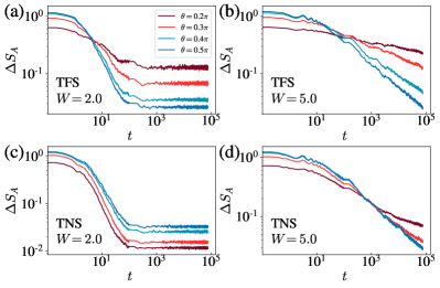
Figure 1: EA dynamics averaged over $100$ different random phases $\phi$ with $N=12$ and $N_{A}=3$. The initial state of (a) and (b) is chosen as TFS and the initial state of (c) and (d) is chosen as TNS. For TFS, the QME always occurs regardless of the choice of $W$. For TNS, the QME only occurs in the MBL phase with $W>W_{c}$.

In the thermal phase with quasiperiodic potential strength $W=2.0<W_{c}$, as shown in Figs. 1 (a) and (c), the QME is present and absent for initial TFS and TNS, respectively. The initial state dependence of the QME in chaotic systems has been observed in the U(1) random circuits [35, 36], which can be understood through the lens of quantum thermalization, i.e., the thermalization speed is slower in the charge sector of smaller Hilbert space. $\rho_{A}$ of the initial TFS and TNS both become more U(1) asymmetric with increasing tilt angle $\theta$. However, for $\rho_{A}$ of TFS, the weights of the smaller charge sectors decrease for larger tilt angle $\theta$, i.e., the more asymmetric initial state has a faster thermalization speed. Consequently, the QME is anticipated. On the contrary, for $\rho_{A}$ of TNS, the weights of the smaller charge sectors increase for larger tilt angle $\theta$, i.e., the more asymmetric initial state has a slower thermalization speed. Therefore, the EA with a more asymmetric initial state remains larger than that with a more symmetric initial state under the quench, and thus the QME is absent.

On the contrary, in the MBL phase with a strong quasiperiodic potential $W=5.0>W_{c}$, the QME always presents regardless of the initial states as shown in Figs. 1 (b) and (d). The symmetry restoration dynamics in the MBL phase are not only distinct from that observed in the thermal phase as discussed above but also show different late-time behaviors compared to that in integrable systems where symmetry cannot be restored for initial TNS [28]. This distinction further underscores the uniqueness and significance of investigating the symmetry restoration and QME in the MBL phase.

It is worth noting that the timescale of the QME (EA crossing between different tilt angles $\theta$) in the MBL phase increases exponentially with the subsystem size due to the logarithmic lightcone [53, 54, 55, 56, 57, 58] while the timescale of the QME in the integrable and chaotic systems is linear in the subsystem size [36, 35, 36]. The symmetry restoration has also been experimentally investigated in a disordered interacting system and the QME is not visible due to the constraint timescale reached [38]. See more numerical results and discussions in the SM [62]. Moreover, it is well-known that the system in the MBL phase keeps a memory of the initial state, e.g., the non-vanishing charge imbalance starting from a Néel state. In other words, quantities such as charge imbalance have the same order with increasing $\theta$ for the initial states and the late time states, contrary to the QME behaviors. The $\theta$ independent symmetry restoration and the order reversing for EA in QME investigated in this Letter is not contrary to this memory characteristic of the MBL phase as EA is a non-local observable and the initial information is encoded in the diagonal part of the disorder averaged late-time subsystem density matrix [62].

Figure 2: EA dynamics in the Anderson localization phase with $V=0$ and $W=2.0$ with initial (a) TFS and (b) TNS. Here, the system size is $N=80$, and the subsystem size is $N_{A}=10$.

In the absence of the interaction $V=0$, $W>2$ for the AA model gives Anderson localization phases. As shown in Fig. 2, the degrees of the symmetry breaking are frozen and the EA remains nearly the same as the initial value. Therefore, both symmetry restoration and QME are absent in the Anderson localization phase. As detailed in the SM [62], the results can also be understood through the effective model of MBL discussed below by setting the coupling $J=0$.

Theoretical analysis.— To analytically understand the distinct behaviors of the symmetry restoration in the MBL phase, we consider the completely diagonalized effective model [61, 60, 86, 87, 88, 89] for the MBL phase under a local unitary transformation

$$H_{\text{eff}}=\sum_{i}h_{i}\tau_{i}^{z}+\sum_{ij}J_{ij}\tau_{i}^{z}\tau_{j}^{z}+\cdots,$$ (6)

where $\tau_{i}^{z}=\sigma_{i}^{z}+\sum_{j,k}\sum_{\alpha,\beta=x,y,z}c^{\alpha,\beta}(i,j,k)\sigma^{\alpha}_{j}\sigma^{\beta}_{k}+\cdots$ are local integrals of motion with $c$ decaying exponentially with the distance between $i$ and $j,k$, $h_{i}$ is uniformly chosen from $[-h,h]$, and $J_{ij}=\tilde{J}_{ij}e^{-|i-j|/\xi}$ with $\tilde{J}_{ij}\in[-J,J]$ and $\xi$ being the localization length. In the following analysis, we further approximate the effective model in the MBL phase shown in Eq. (6) by replacing $\tau^{z}_{i}$ with $\sigma^{z}_{i}$ and neglect the higher-order terms.

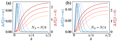
Figure 3: The Rényi-2 EA $\Delta S_{A}^{(2)}$ of the initial state (red) and in the long time limit (blue). $N=[32,64,128,256]$ becomes larger with darker color and $N_{A}=N/8,N/4$ for (a) and (b) respectively. As shown in (a) and (b), there exists a finite peak whose height is unchanged with the increases of system size $N$ [62] indicating a finite size crossover to persistent symmetry broken phase for small $\theta\sim\frac{1}{\sqrt{N}}$.

In the theoretical analysis, we focus on the Rényi-2 EA given by

$$\Delta S_{A}^{(2)}(t)=\log\frac{\tr\rho_{A}^{2}(t)}{\tr\rho_{A,Q}^{2}(t)}.$$ (7)

$\rho_{A}(t)$ and $\rho_{A,Q}(t)$ can both be decomposed into a complete Pauli operator string basis $P^{\bm{\mu}}=\sigma_{0}^{\mu_{0}}\sigma_{1}^{\mu_{1}}\cdots\sigma_{N_{A}-1}^{\mu_{N_{A}-1}}$ where $\sigma_{j}^{\mu_{j}}$ is the $\mu$-type operator on $j$-th site choosing from $\{I_{j},\sigma_{j}^{+},\sigma_{j}^{-},\sigma_{j}^{z}\}$, with upper/lowering operators $\sigma_{j}^{\pm}=\frac{\sigma_{j}^{x}\pm i\sigma_{j}^{y}}{\sqrt{2}}$ that breaks $U(1)$ symmetry [62]. Consequently,

$$\Delta S_{A}^{(2)}(t)=\log\frac{\sum_{\bm{\mu}}|\langle P^{\bm{\mu}}\rangle_{t}|^{2}}{\sum_{\bm{\mu},[P^{\bm{\mu}},Q_{A}]=0}|\langle P^{\bm{\mu}}\rangle_{t}|^{2}},$$ (8)

where the projections in $\rho_{A,Q}$ correspond to discarding the operator strings anti-commute with $Q_{A}$. Subsequently, the calculation for EA is equivalent to evaluating the expectation values of operator strings $P^{\mu}$. In the long time limit $t\to\infty$, we have

$$\Delta S^{(2)}_{A}(t\to\infty,\theta)$$ (9)

$$\approx\log(1+(\frac{1+\cos^{2}(\theta)}{2})^{N-2N_{A}}-(\frac{1+\cos^{2}(\theta)}{2})^{N-N_{A}}),$$

which can be further simplified as

$$\Delta S_{A}^{(2)}(t\to\infty,\theta)\approx\left\{\begin{array}[]{lr}\frac{N_{A}}{2}\theta^{2},\ \ \ \theta\to 0&\\ 0,\ \ \ \ \ \ \ \ \ \theta\to\pi/2.\end{array}\right.$$ (12)

The late-time EA behaviors with varying tilt angle $\theta$ encode the information of both symmetry restoration and QME. On the one hand, zero late-time EA in the thermodynamic limit indicates full symmetry restoration. On the other hand, the monotonic decreasing nature of late-time EA for a range of $\theta$ reflects the presence of QME in the middle times, as the order of EA with respect to $\theta$ is reversed compared to the initial monotonic increasing EA. As shown in Fig. 3, when $N_{A}<N/2$ and tilt angle $\theta$ is large, i.e., the initial state is more U(1) asymmetric, the late-time Rényi-2 EA approaches zero and thus the symmetry can be fully restored in the MBL phase. However, when the tilt angle $\theta$ is sufficiently small, i.e., the initial state is more U(1) symmetric, the late-time Rényi-2 EA is finite and the height of the peak shown in Fig. 3(a)(b) stays the same with increasing system size $N$ while the position of the peak scale with system size as $\theta\sim\frac{1}{\sqrt{N}}$, implying a finite-size crossover for persistent symmetry broken phases. Meanwhile, the late-time monotonic decreasing EA with respect to $\theta$ for $N_{A}<N/2$ indicates the emergence of QME. Notably, the late-time EA results for the effective MBL model are the same for different Hamiltonian parameters and different initial product states, and also quantitatively coincide with the late-time EA results in the quantum chaotic case from TFS [35].

Furthermore, we directly perform numerical simulation of the $\Delta S_{A}^{(2)}$ dynamics under the quench of the effective Hamiltonian shown in Eq. (6). As shown in Fig. 4, the theoretical values in the long time limit agree well with the numerical results, and the QME in the effective model is observed. Moreover, we find the dynamical behaviors are qualitatively consistent with the MBL model in Eq. (Quantum Mpemba effects in many-body localization systems).

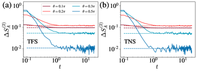
Figure 4: Rényi-2 EA dynamics $\Delta S_{A}^{(2)}(t)$ of the effective model in Eq. (6) with $h=10.0$, $J=10.0$ and $\xi=1.0$. The data is averaged over $100$ disorder realizations. We set $N=12$ and $N_{A}=3$. The initial states of (a) and (b) are the TFS and the TNS respectively. The solid (dashed) line represents the numerical (theoretical late-time) results.

Unlike quantum chaotic quench from TFS and MBL quench from any tilted product states, late-time EA after quantum chaotic quench from other tilted product states beyond ferromagnetic states show distinct behaviors – the symmetry can always be fully restored without finite-size symmetry breaking peak in small $\theta$ [62]. The similarity between MBL quench from any tilted product states with quantum chaotic quench from TFS as well as the difference between quantum chaotic quench from TFS and other tilted product states can be understood in a unified framework, where the key factor is the Hilbert space dimension accessible by the initial product state. In the effective MBL model cases and ferromagnetic initial states cases with charge conservation, the accessible Hilbert space dimensions are both $1$ while for other product states with a fixed ratio of charge under chaotic evolution, the accessible Hilbert space dimensions are exponential. Therefore, in the former case, the effective accessible Hilbert space dimension is still very restricted with small tilt angles $\theta$, rendering persistent symmetry broken in finite size. On the contrary, in the latter case, the exponential large Hilbert space dimension yields sufficient relaxation to equilibrium for all $\theta$. This framework is also compatible with the mechanism for QME in chaotic systems – small charge sectors are hard to thermalize with low equilibration speeds.

Conclusion and outlook.— In this Letter, we investigate the U(1) symmetry restoration in the many-body localization phase. The U(1) symmetry can be fully restored in the MBL phase in an exponential time scale even though MBL forbids thermalization. Interestingly, the presence of the QME is observed in the MBL phase regardless of the choice of the initial tilted product states, which is distinct from the cases in the integrable and chaotic systems. Theoretically, we obtain the analytical results of the entanglement asymmetry for the effective MBL model in the long time limit, which is shown to be independent of the initial product states and consistent with the numerical simulation. Moreover, when the system is finite in size, the late-time subsystem symmetry can not be fully restored and the EA is finite when the tilt angle $\theta$ is sufficiently small while the EA decays to zero when the tilt angle $\theta$ is large. Such late-time behaviors are reminiscent of chaotic quench from TFS, and the opposite monotonicity for EA with respect to $\theta$ between late time and early time supports the presence of the QME.

The mechanism behind the QME in the MBL phase is distinct from that in the integrable and chaotic systems, characterized by different QME timescales and initial state dependence. We have provided a theoretical analysis of the symmetry restoration in the MBL phase stabilized by the strong disorder with the help of the effective model. Besides the strong disorder MBL, other types of MBL such as non-Hermitian MBL [90, 91, 92, 93], MBL with dissipations [94, 95, 96], and the disorder-free Stark MBL [97, 98, 99, 100, 101, 102, 103] have also been extensively investigated. An interesting future direction is to study the symmetry restoration in these different MBL phases, which might deepen our understanding of the MBL.

Acknowledgement.— This work was supported in part by NSFC under Grant No. 12347107 (SL and HY), by MOSTC under Grant No. 2021YFA1400100 (HY), and by the Xplorer Prize through the New Cornerstone Science Foundation (HY). SY is supported by the National Natural Science Foundation of China (Grants No. 12075324 and No. 12222515) and the Science and Technology Projects in Guangdong Province (Grants No. 2021QN02X561).

Supplemental Material for “Quantum Mpemba effects in many-body localization systems”

I Numerical results for many-body localization with random potentials

Besides the many-body localization (MBL) model with quasiperiodic potential, we have also investigated the symmetry restoration and the quantum Mpemba effect (QME) for the MBL model with random potential [46, 45, 74], whose Hamiltonian is given by

$$H= - \sum_{i}(\sigma^{x}_{i}\sigma^{x}_{i+1}+\sigma^{y}_{i}\sigma^{y}_{i+1})+V\sum_{i}\sigma^{z}_{i}\sigma^{z}_{i+1}+\sum_{i}W_{i}\sigma^{z}_{i},$$ (S1)

where random potential $W_{i}\in[0,W]$ with uniform distribution and interaction strength $V$ is fixed to $1/2$. The critical strength of random potential for the many-body localization transition is $W_{c}\approx 9.0$ determined by the crossing of level spacing ratios with different system sizes, see more details in Sec. III.

I.1 Entanglement asymmetry dynamics

The entanglement asymmetry (EA) dynamics with different initial tilted product states and different $W$ are shown in Fig. S1. Similar to the case of the MBL model with quasiperiodic potential investigated in the main text, QMEs are present and absent with initial tilted ferromagnetic state (TFS) and tilted Néel state (TNS) respectively in the thermal phase while QMEs always exist regardless of the choice of the initial states in the MBL phase.

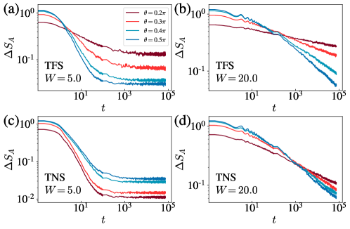
Figure S1: Entanglement asymmetry dynamics with random potential averaged over $100$ disorder realizations. We set $N=12$ and $N_{A}=3$. The initial state of (a) and (b) is TFS and the initial state of (c) and (d) is TNS. For TFS, the QME always occurs regardless of the choice of $W$. For TNS, the QME only occurs in the MBL phase with $W>W_{c}$.

I.2 Charge imbalance dynamics

The local information of the initial state remains in the system even after a long time evolution in the MBL phase due to the memory effects while the local observables become featureless in the thermal phase. For example, the charge imbalance of the initial Néel state [104, 105, 106, 107]

$$\text{CI}(t)=\frac{1}{N}\sum_{i=0}^{N-1}(-1)^{i}\langle\sigma^{z}_{i}\rangle_{t},$$ (S2)

can be utilized to detect the MBL phase. For the TNS investigated in this work with finite initial charge imbalance, we also calculate the charge imbalance dynamics. As shown in Fig. S2 with $N=12$ and $W=20.0$, the charge imbalance remains finite in the late time. Moreover, the order of the charge imbalance with the tilt angle $\theta$ is the same as that for initial states. These properties of local observables are distinct from non-local probs such as EA, which reverses the order with respect to $\theta$ during the quench and finally approaches zero without any memory on the initial EA values.

Figure S2: Charge imbalance dynamics with random potential averaged over $100$ disorder realizations. Here $N=12$ and $W=20.0>W_{c}$.

II Numerical results for power-law decaying XY interacting model with random disorder

The symmetry restoration for the power-law decaying XY interacting model in the presence of random disorder has been experimentally investigated [38]. The Hamiltonian is given by

$$H=\sum_{i>j}\frac{1}{2|i-j|^{\alpha}}(\sigma_{i}^{x}\sigma_{j}^{x}+\sigma_{i}^{y}\sigma_{j}^{y})+\sum_{i}h_{i}\sigma_{i}^{z},$$ (S3)

where $\alpha=1.0$ and $h_{i}\in[0,W]$. The crossing of EA, i.e., the QME, is not visible within the experimental time window in Ref. [38] when the disorder is sufficiently strong. We have also performed additional numerical simulations of the EA dynamics under the quench of the Hamiltonian shown in Eq. (S3) with strong disorder and open boundary conditions. Similar to the model discussed in the main text, the QME always occurs in the MBL phase with large $W$, as shown in Fig. S3. Therefore, the non-visible QME reported in Ref. [38] may be caused by the limited time window. The exponential timescale for the presence of QME in the MBL phase may strictly limit the experimental investigation.

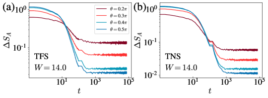
Figure S3: EA dynamics under evolution with Hamiltonian shown in Eq. (S3). The initial state is (a) TFS and (b) TNS. Here $N=12$, $N_{A}=3$ and $W=14.0$.

III Determining many-body localization transition via level spacing ratio

We calculate the level spacing ratio $r$ [108] in the half-filling charge sector to determine the critical $W_{c}$ of the many-body localization transition. The $n$-th level spacing ratio is defined as

$$r_{n}=\frac{\text{min}(\Delta_{n},\Delta_{n+1})}{\text{max}(\Delta_{n},\Delta_{n+1})},$$ (S4)

where $\Delta_{n}=E_{n+1}-E_{n}$ and $E_{n}$ is the $n$-th eigenenergy in ascending order. The level spacing ratio $r$ is the average of $r_{n}$ over different energy level $n$ and different disorder realizations.

The numerical results of the level spacing ratio with random potential are shown in Fig. S4 and the critical strength is $W_{c}\approx 9.0$. The numerical results of the level spacing ratio with quasiperiodic potential are shown in Fig. S5 and the critical strength is $W_{c}\approx 3.3$.

Figure S4: Level spacing ratio in the half-filling sector with random potential. Each data point is averaged over $2000-10000$ disorder realizations. The critical point is $W_{c}\approx 9.0$ determined by the crossing of the level spacing ratios with $N=14$ and $N=16$.

Figure S5: Level spacing ratio in the half-filling sector with quasiperiodic potential. Each data point is averaged over $2000-10000$ disorder realizations. The critical point is $W_{c}\approx 3.3$ determined by the crossing of the level spacing ratios with $N=14$ and $N=16$.

IV Effective model of many-body localization

To make the analytical analysis of the quantum Mpemba effect in the many-body localization phase trackable, we consider the effective Hamiltonian [61, 60, 86, 87, 88, 89] under a local transformation

$$H_{\text{eff}}=\sum_{i}h_{i}\tau_{i}^{z}+\sum_{ij}J_{ij}\tau_{i}^{z}\tau_{j}^{z},$$ (S5)

where $\tau_{i}^{z}=\sigma_{i}^{z}+\sum_{j,k}\sum_{\alpha,\beta=x,y,z}c^{\alpha,\beta}(i,j,k)\sigma^{\alpha}_{j}\sigma^{\beta}_{k}+\cdots$ are local integrals of motion with $c$ decaying exponentially with the distance between $i$ and $j,k$, $h_{i}\in[-h,h]$, and $J_{ij}=\tilde{J}_{ij}e^{-|i-j|/\xi}$ with $\tilde{J}_{ij}\in[-J,J]$ and $\xi$ being the localization length. We further approximate the effective MBL model by replacing $\tau_{i}^{z}$ with $\sigma_{i}^{z}$. In the following sections, we will show the analytical results of symmetry restoration in the Anderson and many-body localization phases based on this effective model.

V Analytical results of $\Delta S_{A}$ in the Anderson localization phase

Before discussing the symmetry restoration and the quantum Mpemba effect in the MBL phase in the following section with the help of the effective model shown in Eq. (S5), we first consider the entanglement asymmetry dynamics with $J=0$, corresponding to the Anderson localization. We choose the tilted ferromagnetic state as the initial state. The evolved state after time $t$

$$|\psi_{\theta}(t)\rangle = e^{-iH_{\text{eff}}t}(\cos(\theta/2)|0\rangle+\sin(\theta/2)|1\rangle)^{\otimes N}$$

$$= \prod_{j=0}^{N-1}(e^{-2ih_{j}t}\cos(\theta/2)|0\rangle+\sin(\theta/2)|1\rangle)_{j},$$

remains a product state, where we have discarded an irrelevant global phase factor. Consequently, $S_{A}=0$ and thus $\Delta S_{A}=S_{A,Q}$. The reduced density matrix of subsystem $A$ of size $N_{A}$ is

$$\rho_{A}(t) = \Tr_{\bar{A}}(|\psi_{\theta}(t)\rangle\langle\psi_{\theta}(t)|)$$

$$= |\psi_{\theta}(t)\rangle_{A}\langle\psi_{\theta}(t)|_{A}$$

$$= \left(\prod_{j=0}^{N_{A}-1}(e^{-2ih_{j}t}\cos(\theta/2)|0\rangle+\sin(\theta/2)|1\rangle)_{j}\right)\left(\prod_{j^{\prime}=0}^{N_{A}-1}(e^{+2ih_{j}t}\cos(\theta/2)\langle 0|+\sin(\theta/2)\langle 1|)_{j^{\prime}}\right),$$

and thus

$$\rho_{A,Q} = \sum_{q}(\Pi_{q}\rho_{A}\Pi_{q})$$

$$= \sum_{q}\cos^{2q}(\theta/2)\sin^{2(N_{A}-q)}(\theta/2)P_{q}O_{q}P^{\dagger}_{q},$$

where $q$ represents the charge in subsystem $A$, $O_{q}=O^{\prime}_{q}\oplus I_{q},$ with $O^{\prime}_{q}$ being a $C_{N_{A}}^{q}\times C_{N_{A}}^{q}$ matrix with all elements being $1$ and $I_{q}$ being a $(2^{N_{A}}-C_{N_{A}}^{q})\times(2^{N_{A}}-C_{N_{A}}^{q})$ identity matrix. We note that the order of the computational basis has been changed for simplicity. $P_{q}$ is the phase matrix of the $q$-th charge sector,

$$P_{q}=\left(\begin{array}[]{cccccc}e^{-2i\sum_{j\in q_{1}}h_{j}t}&&&&&\\ &e^{-2i\sum_{j\in q_{2}}h_{j}t}&&&&\\ &&\ddots&&&\\ &&&e^{-2i\sum_{j\in q_{C_{N_{A}}^{q}}}h_{j}t}&&\\ &&&&0&\\ &&&&&\ddots\\ \end{array}\right)$$ (S15)

where $q_{i}$ is the set of sites with bit $0$ in $i$-th bitstring with charge $q$ in subsystem $A$. Consequently,

$$\rho_{A,Q}(t) = (\sum_{q}P_{q})\rho_{A,Q}(0)(\sum_{q}P_{q})^{\dagger}$$

$$= P\rho_{A,Q}(0)P^{\dagger},$$

where $P$ is a unitary matrix. Therefore, $S_{A,Q}(t)=S_{A,Q}(0)$ and the entanglement asymmetry remains unchanged in the Anderson localization phase, consistent with the numerical results shown in Fig. 4 in the main text.

VI Analytical results in the many-body localization phase

VI.1 Connection between Rényi-2 entanglement asymmetry dynamics and operator spreading

To understand the symmetry restoration and quantum Mpemba effect in many-body localized systems analytically, we can utilize the operator spreading dynamics to quantify the entanglement asymmetry [36]. Following Refs. [109, 110, 36], we introduce a suitable basis for local Hilbert space:

$$\sigma_{i}^{\mu}=\{I_{i},\sigma^{+}_{i},\sigma^{-}_{i},\sigma_{i}^{z}\},$$ (S17)

where $\sigma_{i}^{\pm}=\frac{\sigma_{i}^{x}\pm i\sigma_{i}^{y}}{\sqrt{2}}$ and $\sigma^{x,y,z}_{i}$ are Pauli operators on $i$-th qubit. These operators are traceless and orthogonal under the Frobenius inner product

$$\frac{1}{2}\tr[(\sigma^{\mu}_{i})^{\dagger}\sigma^{\nu}_{j}]=\delta_{ij}\delta^{\mu\nu}.$$ (S18)

The operator string in subsystem $A$ of size $N_{A}$ is denoted as $P^{\bm{\mu}}=\sigma^{\mu_{0}}_{0}\sigma^{\mu_{1}}_{1}\dots\sigma^{\mu_{N_{A}-1}}_{N_{A}-1}$ and $\bm{\mu}=(\mu_{0},\mu_{1},\dots\mu_{N_{A}-1})$. The reduced density matrix $\rho_{A}$ can be decomposed to this operator string basis as

$$\rho_{A}(t)=\frac{1}{2^{N_{A}}}\sum_{\bm{\mu}}\langle(P^{\bm{\mu}})^{\dagger}\rangle_{t}P^{\bm{\mu}}=\frac{1}{2^{N_{A}}}(I+\sum_{\bm{\mu},\bm{\mu}\neq I}\langle(P^{\bm{\mu}})^{\dagger}\rangle_{t}P^{\bm{\mu}}).$$ (S19)

And thus the purity of $\rho_{A}(t)$ is

$$\tr\rho^{2}_{A}(t) = \frac{1}{4^{N_{A}}}\tr\left((I+\sum_{\bm{\mu},\bm{\mu}\neq I}\langle(P^{\bm{\mu}})^{\dagger}\rangle_{t}P^{\bm{\mu}})(I+\sum_{\bm{\nu},\bm{\nu}\neq I}\langle(P^{\bm{\nu}})^{\dagger}\rangle_{t}P^{\bm{\nu}})\right)$$

$$= \frac{1}{2^{N_{A}}}\left(1+\sum_{\bm{\mu},\bm{\mu}\neq I}|\langle P^{\bm{\mu}}\rangle_{t}|^{2}\right)$$

$$= \frac{1}{2^{N_{A}}}\sum_{\bm{\mu}}|\langle P^{\bm{\mu}}\rangle_{t}|^{2}.$$

For $\rho_{A,Q}(t)$, the operators which anti commute with $Q_{A}$ will be discarded because of $[\rho_{A,Q}(t),Q_{A}]=0$ and thus

$$\rho_{A,Q}(t)=\frac{1}{2^{N_{A}}}(I+\sum_{\bm{\mu},\bm{\mu}\neq I,[P^{\bm{\mu}},Q_{A}]=0}\langle(P^{\bm{\mu}})^{\dagger}\rangle_{t}P^{\bm{\mu}}).$$ (S21)

Therefore, the purity of $\rho_{A,Q}(t)$ is

$$\tr\rho^{2}_{A,Q}(t)=\frac{1}{2^{N_{A}}}(1+\sum_{\bm{\mu},\bm{\mu}\neq I,[P^{\bm{\mu}},Q_{A}]=0}|\langle P^{\bm{\mu}}\rangle_{t}|^{2})=\frac{1}{2^{N_{A}}}\sum_{\bm{\mu},[P^{\bm{\mu}},Q_{A}]=0}|\langle P^{\bm{\mu}}\rangle_{t}|^{2}.$$ (S22)

Consequently, the Rényi-2 entanglement asymmetry is

$$\Delta S_{A}^{(2)} = S_{2}(\rho_{A,Q})-S_{2}(\rho_{A})$$

$$= -\log(\tr\rho_{A,Q}^{2})+\log(\tr\rho_{A}^{2})$$

$$= \log\frac{\tr\rho_{A}^{2}}{\tr\rho_{A,Q}^{2}}$$

$$= \log\frac{\sum_{\bm{\mu}}|\langle P^{\bm{\mu}}\rangle_{t}|^{2}}{\sum_{\bm{\mu},[P^{\bm{\mu}},Q_{A}]=0}|\langle P^{\bm{\mu}}\rangle_{t}|^{2}}$$

$$= \log\frac{f(\theta,t)}{f^{c}(\theta,t)},$$

where

$$f(\theta,t) = \sum_{\bm{\mu}}|\langle P^{\bm{\mu}}\rangle_{t}|^{2},$$ (S24)

$$f^{c}(\theta,t) = \sum_{\bm{\mu},[P^{\bm{\mu}},Q_{A}]=0}|\langle P^{\bm{\mu}}\rangle_{t}|^{2},$$

and $\frac{1}{2^{N_{A}}}f(\theta,t)$ is the purity.Having established the connection between the Rényi-2 entanglement asymmetry and operator spreading, we then analytically evaluate the Rényi-2 entanglement asymmetry of different initial states with $t=0$ and the corresponding final steady states in the long time limit $t\rightarrow\infty$.

VI.2 Tilted ferromagnetic state

We first consider the case with the tilted ferromagnetic state as the initial state

$$|\psi_{\theta}\rangle=\prod_{j=0}^{N-1}e^{-i\frac{\theta}{2}\sigma^{y}_{j}}|0\rangle^{\otimes N}=(\cos(\theta/2)|0\rangle+\sin(\theta/2)|1\rangle)^{\otimes N}.$$ (S25)

The operator string with $k$ $\sigma^{+}$ operators, $l$ $\sigma^{-}$ operators and $m$ $\sigma^{z}$ is denoted as $P_{k,l,m}$. For simplicity, we assume

$$P_{k,l,m}=\sigma^{+}_{0}\dots\sigma^{+}_{k-1}\sigma^{-}_{k}\dots\sigma^{-}_{k+l-1}\sigma^{z}_{k+l}\dots\sigma^{z}_{k+l+m-1}I_{k+l+m}\dots I_{N_{A}-1}.$$ (S26)

We choose the computational basis and

$$b = 1_{0}\dots 1_{k-1}0_{k}\dots 0_{k+l-1}\{0,1\}^{N-k-l},$$ (S27)

$$\bar{b} = 0_{0}\dots 0_{k-1}1_{k}\dots 1_{k+l-1}b_{k+l}\dots b_{N-1}$$

are two bitstrings in an $N$-qubit system where bit $0$ corresponds to the presence of a charge. We use $n_{b}$ to represent the number of $1$ in the last $N-k-l$ bits of bitstring $b$. Therefore, the number of 1 in bitstrings $b$ and $\bar{b}$ are $n_{b}+k$ and $n_{b}+l$ respectively. We use $m_{b}$ to represent the number of 1 in $b_{k+l}\dots b_{k+l+m-1}$.

The expectation square of operator string $P_{k,l,m}$ is

$$|\langle\psi_{\theta}|P_{k,l,m}(t)|\psi_{\theta}\rangle|^{2}$$

$$= |\sum_{b}\cos^{2N-2n_{b}-k-l}(\theta/2)\sin^{2n_{b}+k+l}(\theta/2)\langle\bar{b}|e^{iH_{\text{eff}}t}P_{k,l,m}e^{-iH_{\text{eff}}t}|b\rangle|^{2}$$

$$= |\sum_{b}\cos^{2N-2n_{b}-k-l}(\theta/2)\sin^{2n_{b}+k+l}(\theta/2)e^{2i\sum_{i=0}^{k-1}h_{i}t}e^{-2i\sum_{i=k}^{k+l-1}h_{i}t}$$

$$e^{-2i\sum_{i=0}^{k-1}\sum_{j=k+l}^{N-1}J_{ij}(2b_{j}-1)t}e^{-2i\sum_{i=k}^{k+l-1}\sum_{j=k+l}^{N-1}J_{ij}(1-2b_{j})t}\langle\bar{b}|P_{k,l,m}|b\rangle|^{2}$$

$$= |\sum_{b}\cos^{2N-2n_{b}-k-l}(\theta/2)\sin^{2n_{b}+k+l}(\theta/2)e^{-2i\sum_{i=0}^{k-1}\sum_{j=k+l}^{N-1}J_{ij}(2b_{j}-1)t}e^{-2i\sum_{i=k}^{k+l-1}\sum_{j=k+l}^{N-1}J_{ij}(1-2b_{j})t}\langle\bar{b}|P_{k,l,m}|b\rangle|^{2},$$

where we have discarded the global phase factor.

VI.2.1 $\Delta S^{(2)}_{A}$ of the initial tilted ferromagnetic state

When $t=0$, i.e., the initial state,

$$|\langle\psi_{\theta}|P_{k,l,m}(t)|\psi_{\theta}\rangle|^{2} = \left(\sum_{b}\cos^{2N-2n_{b}-k-l}(\theta/2)\sin^{2n_{b}+k+l}(\theta/2)\langle\bar{b}|P_{k,l,m}|b\rangle\right)^{2}$$

$$= 2^{k+l}\left(\sum_{n_{b}=0}^{N-k-l}\cos^{2N-2n_{b}-k-l}(\theta/2)\sin^{2n_{b}+k+l}(\theta/2)(-1)^{m_{b}}\right)^{2}$$

$$= 2^{k+l}\sin^{2k+2l}(\theta/2)\cos^{2k+2l}(\theta/2)$$

$$\left(\sum_{n_{b}-m_{b}=0}^{N-k-l-m}\sum_{m_{b}=0}^{m}C_{m}^{m_{b}}(\cos^{2}(\theta/2))^{N-k-l-m-(n_{b}-m_{b})+m-m_{b}}(\theta/2)(\sin^{2}(\theta/2))^{n_{b}-m_{b}+m_{b}}(-1)^{m_{b}}\right)^{2}$$

$$= 2^{k+l}\sin^{2k+2l}(\theta/2)\cos^{2k+2l}(\theta/2)\left(\sum_{m_{b}=0}^{m}C_{m}^{m_{b}}(\cos^{2}(\theta/2))^{m-m_{b}}(-\sin^{2}(\theta/2))^{m_{b}}\right)^{2}$$

$$= 2^{k+l}\sin^{2k+2l}(\theta/2)\cos^{2k+2l}(\theta/2)(\cos^{2}(\theta/2)-\sin^{2}(\theta/2))^{2m}$$

$$= 2^{-k-l}\sin^{2k+2l}(\theta)\cos^{2m}(\theta).$$

Consequently,

$$f(\theta,0) = \sum_{P^{\bm{\mu}}}|\langle P^{\bm{\mu}}\rangle|^{2}$$

$$= \sum_{k+l=0}^{N_{A}}\sum_{l=0}^{k+l}\sum_{m=0}^{N_{A}-k-l}2^{-k-l}C_{N_{A}}^{k+l}C_{k+l}^{l}C_{N_{A}-k-l}^{m}\sin^{2k+2l}(\theta)\cos^{2m}(\theta)$$

$$= \sum_{k+l=0}^{N_{A}}\sum_{l=0}^{k+l}2^{-k-l}C_{N_{A}}^{k+l}C_{k+l}^{l}\sin^{2k+2l}(\theta)(1+\cos^{2}(\theta))^{N_{A}-k-l}$$

$$= \sum_{k+l=0}^{N_{A}}C_{N_{A}}^{k+l}\sin^{2k+2l}(\theta)(1+\cos^{2}(\theta))^{N_{A}-k-l}$$

$$= 2^{N_{A}},$$

and

$$f^{c}(\theta,0) = \sum_{P^{\bm{\mu}},[P^{\bm{\mu}},Q_{A}]=0}|\langle P^{\bm{\mu}}\rangle|^{2}$$

$$= \sum_{k=0}^{N_{A}/2}\sum_{m=0}^{N_{A}-2k}2^{-2k}C_{N_{A}}^{2k}C_{2k}^{k}C_{N_{A}-2k}^{m}\sin^{4k}(\theta)\cos^{2m}(\theta)$$

$$= \sum_{k=0}^{N_{A}/2}2^{-2k}C_{N_{A}}^{2k}C_{2k}^{k}\sin^{4k}(\theta)(1+\cos^{2}(\theta))^{N_{A}-2k}.$$

Therefore, the Rényi-2 entanglement entropy of the initial tilted ferromagnetic states is

$$\Delta S_{A}^{(2)}(t=0) = \log\frac{f(\theta,0)}{f^{c}(\theta,0)}$$

$$= -\log\sum_{k=0}^{N_{A}/2}2^{-2k-N_{A}}C_{N_{A}}^{2k}C_{2k}^{k}\sin^{4k}(\theta)(1+\cos^{2}(\theta))^{N_{A}-2k}$$

$$= -\log\left(2^{-N_{A}}(1+\cos^{2}(\theta))^{N_{A}}{}_{2}\mathcal{F}_{1}(\frac{1-N_{A}}{2},-\frac{N_{A}}{2},1,\frac{\sin^{4}(\theta)}{(1+\cos^{2}(\theta))^{2}})\right).$$ (S33)

where ${}_{2}\mathcal{F}_{1}(a,b,c,z)$ is hypergeometric function.

VI.2.2 $\Delta S^{(2)}_{A}$ of the steady state

Now, we calculate $\Delta S^{(2)}_{A}$ of the corresponding steady state of the tilted ferromagnetic state. For $P_{k,l,m}$ with $k=l=0$ and thus $[P_{k,l,m},H_{\text{eff}}]=0$,

$$|\langle\psi_{\theta}|P_{0,0,m}(t)|\psi_{\theta}\rangle|^{2}=|\langle\psi_{\theta}|P_{0,0,m}(0)|\psi_{\theta}\rangle|^{2}=\cos^{2m}(\theta).$$ (S34)

If $[P_{k,l,m},H_{\text{eff}}]\neq 0$, the prefactor of the $b-b^{\prime}$ off-diagonal term shown in Eq. (VI.2) is

$$\real(e^{-2i\sum_{i=0}^{k-1}\sum_{j=k+l}^{N-1}J_{ij}(2b_{j}-1)t}e^{-2i\sum_{i=k}^{k+l-1}\sum_{j=k+l}^{N-1}J_{ij}(1-2b_{j})t}$$ (S35)

$$\times e^{2i\sum_{i=0}^{k-1}\sum_{j=k+l}^{N-1}J_{ij}(2b^{\prime}_{j}-1)t}e^{2i\sum_{i=k}^{k+l-1}\sum_{j=k+l}^{N-1}J_{ij}(1-2b^{\prime}_{j})t})=\cos(\phi(J_{i,j},b,b^{\prime})t),$$

which is zero after averaging over different disorder realizations in the long time limit. Therefore,

$$|\langle\psi_{\theta}|P_{k,l,m}(t)|\psi_{\theta}\rangle|^{2} = \sum_{b}\cos^{4N-4n_{b}-2k-2l}(\theta/2)\sin^{4n_{b}+2k+2l}(\theta/2)|\langle\bar{b}|P_{k,l,m}|b\rangle|^{2}$$

$$= 2^{k+l}\sin^{2k+2l}(\theta/2)\cos^{2k+2l}(\theta/2)\sum_{n_{b}=0}^{N-k-l}C_{N-k-l}^{n_{b}}(\cos^{4}(\theta/2))^{N-k-l-n_{b}}(\sin^{4}(\theta/2))^{n_{b}}$$

$$= 2^{k+l}\sin^{2k+2l}(\theta/2)\cos^{2k+2l}(\theta/2)(\cos^{4}(\theta/2)+\sin^{4}(\theta/2))^{N-k-l},$$

Consequently,

$$f(\theta,t\to\infty) = \sum_{P^{\bm{\mu}},k+l>0}|\langle P^{\bm{\mu}}\rangle|^{2}+\sum_{P^{\bm{\mu}},k+l=0}|\langle P^{\bm{\mu}}\rangle|^{2}$$

$$= \sum_{k+l=1}^{N_{A}}\sum_{l=0}^{k+l}2^{N_{A}-k-l}2^{k+l}C_{N_{A}}^{k+l}C_{k+l}^{l}\sin^{2k+2l}(\theta/2)\cos^{2k+2l}(\theta/2)(\cos^{4}(\theta/2)+\sin^{4}(\theta/2))^{N-k-l}+\sum_{m=0}^{N_{A}}C_{N_{A}}^{m}\cos^{2m}(\theta)$$

$$= 2^{N_{A}}\sum_{k^{\prime}=1}^{N_{A}}\sum_{l=0}^{k^{\prime}}C_{N_{A}}^{k^{\prime}}C_{k^{\prime}}^{l}\sin^{2k^{\prime}}(\theta/2)\cos^{2k^{\prime}}(\theta/2)(\cos^{4}(\theta/2)+\sin^{4}(\theta/2))^{N-k^{\prime}}+(1+\cos^{2}(\theta))^{N_{A}}$$

$$= 2^{N_{A}}\sum_{k^{\prime}=1}^{N_{A}}2^{k^{\prime}}C_{N_{A}}^{k^{\prime}}\sin^{2k^{\prime}}(\theta/2)\cos^{2k^{\prime}}(\theta/2)(\cos^{4}(\theta/2)+\sin^{4}(\theta/2))^{N-k^{\prime}}+(1+\cos^{2}(\theta))^{N_{A}}$$

$$= 2^{N_{A}}\sum_{k^{\prime}=0}^{N_{A}}2^{k^{\prime}}C_{N_{A}}^{k^{\prime}}\sin^{2k^{\prime}}(\theta/2)\cos^{2k^{\prime}}(\theta/2)(\cos^{4}(\theta/2)+\sin^{4}(\theta/2))^{N-k^{\prime}}$$

$$-2^{N_{A}}(\cos^{4}(\theta/2)+\sin^{4}(\theta/2))^{N}+(1+\cos^{2}(\theta))^{N_{A}}$$

$$= 2^{N_{A}}((\cos^{4}(\theta/2)+\sin^{4}(\theta/2))^{N-N_{A}}-(\cos^{4}(\theta/2)+\sin^{4}(\theta/2))^{N})+(1+\cos^{2}(\theta))^{N_{A}}$$

$$= 2^{2N_{A}-N}(1+\cos^{2}(\theta))^{N-N_{A}}-2^{N_{A}-N}(1+\cos^{2}(\theta))^{N}+(1+\cos^{2}(\theta))^{N_{A}}$$

$$= 2^{N_{A}}\left(((\frac{1+\cos^{2}(\theta)}{2})^{N-N_{A}}-1)(1-(\frac{1+\cos^{2}(\theta)}{2})^{N_{A}})+1\right).$$

When $N_{A}=N$, $f(\theta,t\to\infty)=2^{N}$ and thus the purity $\frac{1}{2^{N}}f(\theta,t\to\infty)$ is $1$, consistent with the fact that the whole system is still a pure state. For the $f_{c}$,

$$f^{c}(\theta,t\to\infty) = \sum_{P^{\bm{\mu}},[P^{\bm{\mu}},Q_{A}]=0,k+l>0}|\langle P^{\bm{\mu}}\rangle|^{2}+(1+\cos^{2}(\theta))^{N_{A}}$$

$$= \sum_{2k=2}^{N_{A}}2^{N_{A}-2k}2^{2k}C_{N_{A}}^{2k}C_{2k}^{k}\sin^{4k}(\theta/2)\cos^{4k}(\theta/2)(\cos^{4}(\theta/2)+\sin^{4}(\theta/2))^{N-2k}+(1+\cos^{2}(\theta))^{N_{A}}$$

$$= 2^{N_{A}}\sum_{k=1}^{N_{A}/2}C_{N_{A}}^{2k}C_{2k}^{k}\sin^{4k}(\theta/2)\cos^{4k}(\theta/2)(\cos^{4}(\theta/2)+\sin^{4}(\theta/2))^{N-2k}+(1+\cos^{2}(\theta))^{N_{A}}$$

$$= 2^{N_{A}}\sum_{k=1}^{N_{A}/2}C_{N_{A}}^{2k}C_{2k}^{k}2^{-4k}\sin^{4k}(\theta)(\frac{1+\cos^{2}(\theta)}{2})^{N-2k}+(1+\cos^{2}(\theta))^{N_{A}}$$

$$= 2^{N_{A}}\left(\sum_{k=1}^{N_{A}/2}C_{N_{A}}^{2k}C_{2k}^{k}2^{-4k}\sin^{4k}(\theta)(\frac{1+\cos^{2}(\theta)}{2})^{N-2k}+(\frac{1+\cos^{2}(\theta)}{2})^{N_{A}}\right)$$

$$= 2^{N_{A}}(\frac{1+\cos^{2}(\theta)}{2})^{N_{A}}\left(\sum_{k=1}^{N_{A}/2}C_{N_{A}}^{2k}C_{2k}^{k}2^{-4k}\sin^{4k}(\theta)(\frac{1+\cos^{2}(\theta)}{2})^{N-N_{A}-2k}+1\right).$$

In the thermodynamic limit $N\to\infty$ and $N_{A}/N<1/2$,

$$\sum_{k=1}^{N_{A}/2}C_{N_{A}}^{2k}C_{2k}^{k}2^{-4k}\sin^{4k}(\theta)(\frac{1+\cos^{2}(\theta)}{2})^{N-N_{A}-2k} \leq \left(\sum_{k=1}^{N_{A}/2}C_{N_{A}}^{2k}C_{2k}^{k}2^{-4k}\sin^{4k}(\theta)\right)(\frac{1+\cos^{2}(\theta)}{2})^{N-2N_{A}}$$

$$\ll 1,$$

and

$$f^{c}(\theta,t\to\infty) \approx 2^{N_{A}}(\frac{1+\cos^{2}(\theta)}{2})^{N_{A}}.$$ (S40)

Therefore, the Rényi-2 entanglement asymmetry in the long time limit is

$$\Delta S_{A}^{(2)} \approx \log\frac{2^{N_{A}}\left(((\frac{1+\cos^{2}(\theta)}{2})^{N-N_{A}}-1)(1-(\frac{1+\cos^{2}(\theta)}{2})^{N_{A}})+1\right)}{2^{N_{A}}(\frac{1+\cos^{2}(\theta)}{2})^{N_{A}}}$$

$$= \log\left(1+(\frac{1+\cos^{2}(\theta)}{2})^{N-2N_{A}}-(\frac{1+\cos^{2}(\theta)}{2})^{N-N_{A}}\right).$$

The theoretical results of the Rényi-2 entanglement asymmetry of initial states and steady states are shown in Fig. 3 in the main text.

Now, we consider some limits. In the $\theta\to 0$ limit, $\frac{1+\cos^{2}(\theta)}{2}\approx 1-\frac{\theta^{2}}{2}$ and thus

$$\Delta S_{A}^{(2)}\approx\log(1+N_{A}\theta^{2}/)\approx\frac{N_{A}\theta^{2}}{2}.$$ (S42)

In the $\theta\to\pi/2$ limit, $\frac{1+\cos^{2}(\theta)}{2}\approx\frac{1+\delta\theta^{2}}{2}$ where $\delta\theta=\pi/2-\theta$ and thus

$$\Delta S_{A}^{(2)}\approx\log 1=0.$$ (S43)

Consequently, when $N_{A}/N<1/2$,

$$\Delta S_{A}^{(2)}(\theta)=\left\{\begin{aligned} \frac{N_{A}}{2}\theta^{2},\ \ \ \theta\to 0\\ 0,\ \ \ \ \theta\to\pi/2,\end{aligned}\right.$$ (S44)

which indicates the existence of the quantum Mpemba effect as the monotonic decreasing nature of late-time EA following the two limits.

VI.3 Tilted Néel state

Now, we consider the case with the tilted Néel state as the initial state

$$|\psi_{\theta}\rangle=\prod_{j=0}^{N-1}e^{-i\frac{\theta}{2}\sigma^{y}_{j}}(\sigma^{x}_{j})^{j}|0\rangle^{\otimes N}=(\cos(\theta/2)|0\rangle+\sin(\theta/2)|1\rangle)_{\text{even}}^{\otimes N/2}\otimes(-\sin(\theta/2)|0\rangle+\cos(\theta/2)|1\rangle)_{\text{odd}}^{\otimes N/2}.$$ (S45)

The operator string with $k^{e}$ $\sigma^{+}$, $l^{e}$ $\sigma^{-}$, $m^{e}$ $\sigma^{z}$ on even sites and $k^{o}$ $\sigma^{+}$, $l^{o}$ $\sigma^{-}$, $m^{o}$ $\sigma^{z}$ on odd sites is denoted as $P_{(k,l,m)^{e},(k,l,m)^{o}}$. For simplicity, we assume,

$$P_{(k,l,m)^{e},(k,l,m)^{o}}=P_{(k,l,m)^{e}}P_{(k,l,m)^{o}},$$ (S46)

where

$$P_{(k,l,m)^{e}} = \sigma^{+}_{0}\dots\sigma^{+}_{2k^{e}-2}\sigma^{-}_{2k^{e}}\dots\sigma^{-}_{2k^{e}+2l^{e}-2}\sigma^{z}_{2k^{e}+2l^{e}}\dots\sigma^{z}_{2k^{e}+2l^{e}+2m^{e}-2}I_{2k^{e}+2l^{e}+2m^{e}}\dots I_{N-2},$$ (S47)

$$P_{(k,l,m)^{o}} = \sigma^{+}_{1}\dots\sigma^{+}_{2k^{o}-1}\sigma^{-}_{2k^{o}+1}\dots\sigma^{-}_{2k^{o}+2l^{o}-1}\sigma^{z}_{2k^{o}+2l^{o}+1}\dots\sigma^{z}_{2k^{o}+2l^{o}+2m^{o}-1}I_{2k^{o}+2l^{o}+2m^{o}+1}\dots I_{N-1}.$$ (S48)

Suppose

$$b=b^{e}b^{o}=\left(1_{0}\dots 1_{2k^{e}-2}0_{2k^{e}}\dots 0_{2k^{e}+2l^{e}-2}\{0,1\}^{N/2-k^{e}-l^{e}}\right)\left(1_{1}\dots 1_{2k^{o}-1}0_{2k^{o}+1}\dots 0_{2k^{o}+2l^{o}-1}\{0,1\}^{N/2-k^{o}-l^{o}}\right)$$ (S49)

and

$$\bar{b}=\bar{b}^{e}\bar{b}^{o},$$ (S50)

with

$$\bar{b}^{e} = 0_{0}\dots 0_{2k^{e}-2}1_{2k^{e}}\dots 1_{2k^{e}+2l^{e}-2}b_{2k^{e}+2l^{e}}\dots b_{N-2},$$ (S51)

$$\bar{b}^{o} = 0_{1}\dots 0_{2k^{o}-1}1_{2k^{o}+1}\dots 1_{2k^{o}+2l^{o}-1}b_{2k^{o}+2l^{o}+1}\dots b_{N-1}.$$ (S52)

We use $n_{b}^{e(o)}$ to represent the number of $1$ in the last $N/2-k^{e(o)}-l^{e(o)}$ of $b^{e(o)}$ and $m_{b}^{e(o)}$ to represent the number of $1$ in the $b_{2k^{e}+2l^{e}}\dots b_{2k^{e}+2l^{e}+2m^{e}-2}$ $(b_{2k^{o}+2l^{o}+1}\dots b_{2k^{o}+2l^{o}+2m^{o}-1})$.

The expectation square of operator string $P_{(k,l,m)^{e},(k,l,m)^{o}}$ is

$$|\langle\psi_{\theta}|P_{(k,l,m)^{e},(k,l,m)^{o}}(t)|\psi_{\theta}\rangle|^{2}$$

$$= |\sum_{b}\cos^{(\frac{N}{2}-k^{e}-n_{b}^{e})+(k^{o}+n_{b}^{o})+(\frac{N}{2}-l^{e}-n_{b}^{e})+(l^{o}+n_{b}^{o})}(\theta/2)\sin^{(k^{e}+n_{b}^{e})+(\frac{N}{2}-k^{o}-n_{b}^{o})+(l^{e}+n_{b}^{e})+(\frac{N}{2}-l^{o}-n_{b}^{o})}(\theta/2)$$

$$(-1)^{(\frac{N}{2}-k^{o}-n_{b}^{o})+(\frac{N}{2}-l^{o}-n_{b}^{o})}R(t)\langle\bar{b}|P_{(k,l,m)^{e},(k,l,m)^{o}}|b\rangle|^{2},$$

where $R(t)$ is the phase factor.

VI.3.1 $\Delta S_{A}^{(2)}$ of the initial tilted Néel state

When $t=0$,

$$|\langle\psi_{\theta}|P_{(k,l,m)^{e},(k,l,m)^{o}}(t)|\psi_{\theta}\rangle|^{2} = (\sum_{b}\cos^{(\frac{N}{2}-k^{e}-n_{b}^{e})+(k^{o}+n_{b}^{o})+(\frac{N}{2}-l^{e}-n_{b}^{e})+(l^{o}+n_{b}^{o})}(\theta/2)$$

$$\sin^{(k^{e}+n_{b}^{e})+(\frac{N}{2}-k^{o}-n_{b}^{o})+(l^{e}+n_{b}^{e})+(\frac{N}{2}-l^{o}-n_{b}^{o})}(\theta/2)$$

$$(-1)^{(\frac{N}{2}-k^{o}-n_{b}^{o})+(\frac{N}{2}-l^{o}-n_{b}^{o})}\langle\bar{b}|P_{(k,l,m)^{e},(k,l,m)^{o}}|b\rangle)^{2}$$

$$= 2^{-k^{e}-l^{e}-k^{o}-l^{o}}\sin^{2k^{e}+2l^{e}+2k^{o}+2l^{o}}(\theta)\cos^{2m^{e}+2m^{o}}(\theta)$$

$$= 2^{-k-l}\sin^{2(k+l)}(\theta)\cos^{2m}(\theta),$$

which is the same as that with the tilted ferromagnetic state as shown in Eq. (VI.2.1). Moreover, due to Vandermonde’s identity, the Rényi-2 entanglement asymmetry obtained by summing the expectation square of operator strings is the same as that of the tilted ferromagnetic state.

VI.3.2 $\Delta S^{(2)}_{A}$ of the steady state

For $P_{(k,l,m)^{e},(k,l,m)^{o}}$ with $k^{e}=l^{e}=k^{o}=l^{o}=0$ and thus $[P_{(k,l,m)^{e},(k,l,m)^{o}},H_{\text{eff}}]=0$

$$|\langle\psi_{\theta}|P_{(k,l,m)^{e},(k,l,m)^{o}}(t)|\psi_{\theta}\rangle|^{2} = |\langle\psi_{\theta}|P_{(k,l,m)^{e},(k,l,m)^{o}}(0)|\psi_{\theta}\rangle|^{2}$$

$$= 2^{-k^{e}-l^{e}-k^{o}-l^{o}}\sin^{2k^{e}+2l^{e}+2k^{o}+2l^{o}}(\theta)\cos^{2m^{e}+2m^{o}}(\theta).$$

If $[P_{(k,l,m)^{e},(k,l,m)^{o}},H_{\text{eff}}]\neq 0$ , in the long time limit, all off-diagonal terms vanish after averaging over different disorder realizations and thus

$$|\langle\psi_{\theta}|P_{(k,l,m)^{e},(k,l,m)^{o}}(t)|\psi_{\theta}\rangle|^{2}$$

$$= \sum_{b}\cos^{2((\frac{N}{2}-k^{e}-n_{b}^{e})+(k^{o}+n_{b}^{o})+(\frac{N}{2}-l^{e}-n_{b}^{e})+(l^{o}+n_{b}^{o}))}(\theta/2)\sin^{2((k^{e}+n_{b}^{e})+(\frac{N}{2}-k^{o}-n_{b}^{o})+(l^{e}+n_{b}^{e})+(\frac{N}{2}-l^{o}-n_{b}^{o}))}(\theta/2)\langle\bar{b}|P_{(k,l,m)^{e},(k,l,m)^{o}}|b\rangle^{2}$$

$$= 2^{-k^{e}-l^{e}-k^{o}-l^{o}}\sin^{2(k^{e}+l^{e}+k^{o}+l^{o})}(\theta)(\sin^{4}(\theta/2)+\cos^{4}(\theta/2))^{N-k^{e}-l^{e}-k^{o}-l^{o}},$$

which is the same as that of the tilted ferromagnetic state as shown in Eq. (VI.2.2). Therefore, the late-time Rényi-2 entanglement asymmetry of the tilted Néel states is also the same as that of the tilted ferromagnetic state and thus the QME is anticipated, consistent with the numerical results shown in the main text.

VI.4 General tilted product state

Besides two typical initial states focused on in the main text, the analytical analysis above can be easily extended to the cases with other tilted product states. More importantly, the Rényi-2 entanglement asymmetry is the same and independent of the choice of initial tilted product states. Suppose there are $N_{0}$ 0-bits and $N_{1}$ 1-bits in the product state before tilted. In the analytical analysis above for the tilted Néel state, the bits on even sites are $0$ and thus $N_{0}=N_{e}=N/2$, and the bits on odd sites are $1$ and thus $N_{1}=N_{o}=N/2$. We can also define the string operator $P_{(k,l,m)^{0},(k,l,m)^{1}}$ similar to the case of tilted Néel state and the analytical results of Rényi-2 entanglement asymmetry can be obtained by replacing $(k,l,m)^{e}$ and $(k,l,m)^{o}$ with $(k,l,m)^{0}$ and $(k,l,m)^{1}$ respectively. Consequently, the Rényi-2 entanglement at $t=0$ and in the long time limit are both independent of the choice of the initial states. This initial state independence is significantly different from the cases in integrable and chaotic systems.

We now focus on the late-time density matrix structure of MBL evolution, which should be symmetric but not in thermal equilibrium. As mentioned in the main text, the MBL system keeps the memory of the local observable of the initial state in the time evolution. A natural question arises as what is the disorder averaged density matrix describing the system in the long time limit? We demonstrate the disorder averaged late-time state $\rho_{A}(t\rightarrow\infty)$ with the initial tilted ferromagnetic state and the extension to other initial states is straightforward. As shown in Eq. (S19), the reduced density matrix $\rho_{A}$ for each given disorder configuration can be decomposed into the operator string basis. Due to the random phase factor in $\langle P_{k,l,m}^{\dagger}\rangle$ as shown in Eq. (VI.2), only the operator string $P_{k,l,m}$ with $k=l=0$ has non-zero contribution with diagonal terms to the reduced density matrix $\rho_{A}$ after the disorder average. Because $P_{0,0,m}$ commute with the effective Hamiltonian, its expectation value, i.e., the diagonal term in $\rho_{A}(t)$, remains the same as that of the initial state. Consequently, the system with the initial tilted ferromagnetic state in the long time limit is described by

$$\rho_{A}(t\rightarrow\infty)=\begin{pmatrix}\cos^{2}(\theta/2)&0\\ 0&\sin^{2}(\theta/2)\end{pmatrix}^{\otimes N_{A}}.$$ (S57)

This result is consistent with the memory effect of local observable in the MBL phase and presents a natural setting where long-time evolved state restores the symmetry but not approaches thermal equilibrium.

VII Entanglement asymmetry in random unitary circuits with different initial states

We extend the analysis in our previous work [35] to give analytical late-time entanglement asymmetry results for different tilted product states beyond tilted ferromagnetic states in U(1)-symmetric random circuits, i.e. quantum chaotic systems with charge conservation.

We denote $\nu$ as the 1-doping level for a product state, i.e., the ratio of the number of qubits in $\ket{1}$ over the total qubits $N$. Thus, $\nu=0$ (or $\nu=1$) corresponds to the ferromagnetic state and $\nu=1/2$ corresponds to the Néel state. Suppose $N\nu$ is an integer, giving the total number of $1$ in the product states. If the initial state $\rho_{0}$ takes the form of the $Y$-tilted product state with $N\nu$ qubits originally in $\ket{1}$

$$e^{-\frac{i}{2}\sum_{j}\sigma^{y}_{j}\theta}\ket{0}^{\otimes N(1-\nu)}\otimes\ket{1}^{\otimes N\nu} =\left(\cos\frac{\theta}{2}\ket{0}+\sin\frac{\theta}{2}\ket{1}\right)^{\otimes N(1-\nu)}\left(-\sin\frac{\theta}{2}\ket{0}+\cos\frac{\theta}{2}\ket{1}\right)^{\otimes N\nu}$$ (S58)

$$=\sum_{b}\left(\cos\frac{\theta}{2}\right)^{N(1-\nu)-q_{0}(b)+q_{1}(b)}\left(\sin\frac{\theta}{2}\right)^{q_{0}(b)}\left(-\sin\frac{\theta}{2}\right)^{N\nu-q_{1}(b)}\ket{b},$$

where $b$ runs over all $01$-bit strings of length $N$. $q_{0}(b)$ and $q_{1}(b)$ count the number of $1$ in $b$ for the qubits originally in $\ket{0}$ and $\ket{1}$ in the untilted initial product state, respectively. Denote $\Pi_{q}$ as the projector onto the $q$-charge sector of the whole system. Then the weight of the initial state $\rho_{0}$ in the $q$-charge sector is

$$\tr(\rho_{0}\Pi_{q}) =\sum_{b}\left(\cos^{2}\frac{\theta}{2}\right)^{N(1-\nu)-q_{0}(b)+q_{1}(b)}\left(\sin^{2}\frac{\theta}{2}\right)^{q_{0}(b)+N\nu-q_{1}(b)}\bra{b}\Pi_{q}\ket{b}$$ (S59)

$$=\sum_{b}\left(\cos^{2}\frac{\theta}{2}\right)^{N(1-\nu)-(q_{0}(b)-q_{1}(b))}\left(\sin^{2}\frac{\theta}{2}\right)^{N\nu+(q_{0}(b)-q_{1}(b))}\delta_{q_{0}(b)+q_{1}(b),q}$$

$$=\sum_{q_{0}=0}^{q}C_{N(1-\nu)}^{q-q_{0}}C_{N\nu}^{q_{0}}\left(\cos^{2}\frac{\theta}{2}\right)^{N(1-\nu)-(q_{0}-q_{1})}\left(\sin^{2}\frac{\theta}{2}\right)^{N\nu+(q_{0}-q_{1})}.$$

One can check that the number of terms is consistent by using the Chu–Vandermonde identity of binomial coefficients

$$\sum_{q_{0}=0}^{q}C_{N(1-\nu)}^{q-q_{0}}C_{N\nu}^{q_{0}}=C_{N}^{q}.$$ (S60)

By the derivation in Ref. [35], the average purity of the reduced density matrix $\rho_{A}$ of the late-time evolved state on the subsystem of size $N_{A}$ can be expressed as

$$\mathbb{E}_{\mathbb{U}}[\tr(\rho_{A}^{2})] =\sum_{q\neq p}\frac{\tr(\rho_{0}\Pi_{q})\tr(\rho_{0}\Pi_{p})}{C_{N}^{q}C_{N}^{p}}\left[f(q,p,N_{A},N_{\bar{A}})+f(q,p,N_{\bar{A}},N_{A})\right]$$ (S61)

$$\quad+\sum_{q}\frac{\tr(\rho_{0}\Pi_{q})^{2}}{C_{N}^{q}(C_{N}^{q}+1)}\left[f(q,q,N_{A},N_{\bar{A}})+f(q,q,N_{\bar{A}},N_{A})\right],$$

where the $f$-factor is

$$f(q,p,N_{A},N_{\bar{A}})=\sum_{q^{\prime}=0}^{\min\{q,p\}}C_{N_{\bar{A}}}^{q-q^{\prime}}C_{N_{\bar{A}}}^{p-q^{\prime}}C_{N_{A}}^{q^{\prime}}.$$ (S62)

Similarly, the average purity of the pruned state $\rho_{A,Q}$ is

$$\mathbb{E}_{\mathbb{U}}[\tr(\rho_{A,Q}^{2})] =\sum_{q\neq p}\frac{\tr(\rho_{0}\Pi_{q})\tr(\rho_{0}\Pi_{p})}{C_{N}^{q}C_{N}^{p}}f(q,p,N_{A},N_{\bar{A}})$$ (S63)

$$\quad+\sum_{q}\frac{\tr(\rho_{0}\Pi_{q})^{2}}{C_{N}^{q}(C_{N}^{q}+1)}\left[f(q,q,N_{A},N_{\bar{A}})+f(q,q,N_{\bar{A}},N_{A})\right].$$

Based on the expressions above, one can compute the entanglement asymmetry efficiently by summing over certain products of binomial coefficients.

As shown in Fig. S6, we fix $N_{A}/N=1/3$ and compute the average Rényi-2 entanglement asymmetry $\mathbb{E}[\Delta S_{A}^{(2)}]$ for different system size $N$, tilt angle $\theta$, and $1$-doping level $\nu$. At $\nu=0$ where the initial state is a tilted ferromagnetic state, with increasing $N$, the curve of $\mathbb{E}[\Delta S_{A}^{(2)}]$ vs $\theta$ converges to a Gaussian-like peak with constant height and gradually leftward-shifted position of $1/\sqrt{N}$ scaling [35]. That is to say, for a largely tilted ferromagnetic initial state, the symmetry is restored easily and thoroughly while for a slightly tilted one, the symmetry cannot be restored prominently for a finite-size system in the long-time limit, which can be seen as an indicator of the quantum Mpemba effect.

By contrast, at $\nu>0$ where the initial state is still a tilted product state but with proportionable qubits in $\ket{0}$ and $\ket{1}$ ($\nu=1/2$ for the tilted Néel state), with increasing $N$, the overall magnitude of the curve of $\mathbb{E}[\Delta S_{A}^{(2)}]$ vs $\theta$ decays very fast and becomes featureless and flat at zero. More specifically, as shown by the fitting results in Fig. S7, the maximum of the curve decays exponentially with the system size $N$ for $\nu>0$ while is constant for $\nu=0$. In other words, the symmetry is restored for $\nu>0$ regardless of the values of the tilt angle $\theta$. This can be partially understood by the fact that the Hilbert space dimension for any charge sector corresponding to $\nu>0$ scales exponentially with $N$ ($C_{N}^{N\nu}$) while it is a constant $1$ for $\nu=0$, greatly limiting the occurrence of quantum thermalization.

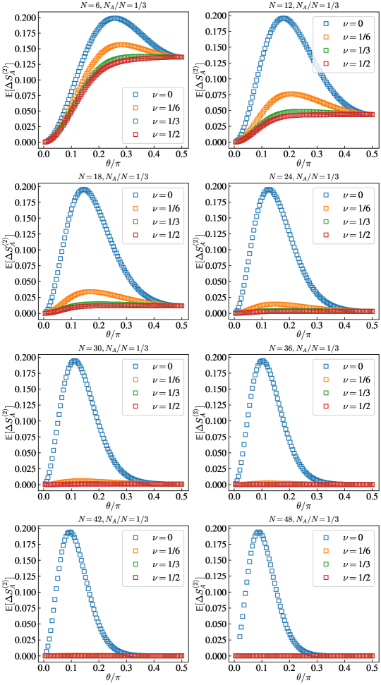
Figure S6: The average Rényi-2 entanglement entropy as a function of the tilt angle $\theta$ for product initial states with different $1$-doping level $\nu$ and different system sizes $N$ with $N_{A}/N=1/3$.

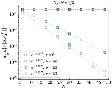
Figure S7: The maximum of the average Rényi-2 entanglement entropy (peak height) as a function of $N$ with $N_{A}/N=1/3$ for product initial states with different $1$-doping level $\nu$.