From Halos to Galaxies. X: Decoding Galaxy SEDs with Physical Priors and Accurate Star Formation History Reconstruction

Abstract

The spectral energy distribution (SED) of galaxies is essential for deriving fundamental properties like stellar mass and star formation history (SFH). However, conventional methods, including both parametric and non-parametric approaches, often fail to accurately recover the observed cosmic star formation rate (SFR) density due to oversimplified or unrealistic assumptions about SFH and their inability to account for the complex SFH variations across different galaxy populations. To address this issue, we introduce a novel approach that improves galaxy broad-band SED analysis by incorporating physical priors derived from hydrodynamical simulations. Tests using IllustrisTNG simulations demonstrate that our method can reliably determine galaxy physical properties from broad-band photometry, including stellar mass within 0.05 dex, current SFR within 0.3 dex, and fractional stellar formation time within 0.2 dex, with a negligible fraction of catastrophic failures. When applied to the SDSS main photometric galaxy sample with spectroscopic redshift, our estimates of stellar mass and SFR are consistent with the widely-used MPA-JHU and GSWLC catalogs. Notably, using the derived SFHs of individual SDSS galaxies, we estimate the cosmic SFR density and stellar mass density with remarkable consistency to direct observations up to $z\sim 6$. This marks the first time SFHs derived from SEDs can accurately match observations. Consequently, our method can reliably recover observed spectral indices such as $\rm D_{\rm n}(4000)$ and $\rm H\delta_{\rm A}$ by synthesizing the full spectra of galaxies using the estimated SFHs and metal enrichment histories, relying solely on broad-band photometry as input. Furthermore, this method is extremely computationally efficient compared to conventional approaches.

1 Introduction

The spectral energy distribution (SED) of galaxies encodes valuable information on a number of astrophysical processes of galaxy evolution, including gas inflow, star formation, gas outflow, and chemical enrichment. Extracting this information effectively from galaxy SEDs is a central challenge in understanding galaxy formation and evolution (see Conroy, 2013, for a review). Traditional approaches typically involve forward-modeling the synthesized SED and adjusting model parameters to fit the observed data of a galaxy.

Deriving accurate star formation history (SFH) is one of the holy grails in SED fitting. Currently, the most widely used tools for obtaining SFH through SED fitting are Bagpipes (Carnall et al., 2018, 2019) and Prospector (Johnson et al., 2021; Leja et al., 2019). Despite its utility, the SED alone often fails to tightly constrain SFHs due to degeneracies among the effects of different stellar ages, metallicities, and dust extinction (Faber, 1972; O’Connell, 1976; Worthey et al., 1994; Carnall et al., 2019; Papovich et al., 2001) and the outshining problem (i.e., young stars outshine their older counterparts, making it hard to constrain the old stellar populations from SEDs, Papovich et al., 2001). Observational limitations such as restricted wavelength coverage and low signal-to-noise ratios further complicate this issue.

Strong priors have been implemented on the SFHs to mitigate these challenges. Common approaches include parametric models like the exponential model $(\propto e^{-(t-t_{0})/\tau})$, which is also known as the $\tau$ model and was widely used, perhaps for being the result of the closed-box model in which the star formation rate (SFR) is proportional to the gas mass (Schmidt, 1959), which is assumed to be all in place at the beginning. This is not what happens to real galaxies, which start from small seeds and grow secularly by merging and gas accretion. Moreover, a single function is incapable of capturing features from recent starbursts and to cope with this, additional burst components were incorporated (Kauffmann et al., 2003; Lee et al., 2009). In an attempt to use more realistic SFHs, exponentially rising ($\propto e^{(t-t_{0})/\tau}$) and delayed-exponential ($\propto(t-t_{0})e^{-(t-t_{0})/\tau}$) were introduced (Maraston et al., 2010; Lee et al., 2010). Motivated by the coverage of observational parameter space of spatially resolved spectra from the Calar Alto Legacy Integral Field Area (CALIFA) survey (Sánchez et al., 2012), library of SFHs modeled as double-gaussian plus random burst was also applied (see Zibetti et al., 2017, 2020, as well as high redshift application in preparation). Motivated by the shape of the cosmic SFR density (Madau & Dickinson, 2014), the $\Gamma$ function was also used in the SED fits (Lu et al., 2015; Zhou et al., 2020); with others preferring the log-normal function or a double power-law (see Gladders et al., 2013; Abramson et al., 2016; Diemer et al., 2017; Carnall et al., 2018). Finally, to increase flexibility, the combination of different functions is sometimes also applied (e.g., Carnall et al., 2018; Han et al., 2023).

Clearly, there is no guarantee that galaxies have evolved following any of these simple analytical functions, that introduce arbitrary non-physical priors (Simha et al., 2014; Carnall et al., 2019). Consequently, models based on the non-parametric SFHs have also been employed (Cid Fernandes et al., 2005; Ocvirk et al., 2006; Leja et al., 2017; Iyer & Gawiser, 2017; Chauke et al., 2018; Iyer et al., 2019). Regarding the limited ability to constrain the detailed shape of star formation histories, these non-parametric methods adopted broad step functions with additional continuity requirement (Cappellari, 2012; Walcher et al., 2015; Leja et al., 2017, 2019). Although these non-parametric methods can successfully recover simple artificially input SFHs (Leja et al., 2019), realistic SFHs of actual galaxies are still challenging. Moreover, non-parametric methods suffer from various degeneracies, are computationally demanding and require high-quality data to constrain SFHs.

A promising solution to these limitations involves leveraging physical priors from realistic galaxy formation models. These models, including empirical models (e.g. Conroy & Wechsler, 2009; Moster et al., 2010; Yang et al., 2012; Behroozi et al., 2019; Chen et al., 2021), semi-analytic models (e.g. White & Frenk, 1991; Kauffmann et al., 1993; Somerville & Primack, 1999; Guo et al., 2011), and hydrodynamical simulations (e.g. Katz et al., 1992; Crain et al., 2009; Pillepich et al., 2018a; Schaye et al., 2015, 2023), should be realistic in the sense that they are capable of reproducing various distribution functions and scaling relations for observed galaxies. Using these models’ star formation and metal enrichment histories, it is possible to establish more physically grounded priors for inferring real galaxy histories from SEDs. Similar approaches have been put into practice in Pacifici et al. (2012), where they use a semi-analytic galaxy formation model as a prior to infer the physical properties from galaxy observables (see also Finlator et al., 2007; Pacifici et al., 2016). Recently, Zhou et al. (2022) incorporate the semi-analytic model of galaxy evolution processes, including inflow, outflow, star formation and chemical enrichment (Talbot & Arnett, 1971; Tinsley, 1974; Chiosi, 1980; Tinsley, 1980; Lacey & Fall, 1985; Bouché et al., 2010; Lilly et al., 2013; Dekel et al., 2013; Peng & Maiolino, 2014; Dekel & Mandelker, 2014; Dou et al., 2021; Wang & Lilly, 2021, 2022), into the modelling of galaxy spectra.

This work utilizes the SFHs and metal enrichment histories of realistic galaxies in state-of-the-art hydrodynamical simulations to infer the physical properties of observed galaxies from their broad-band photometry. We demonstrate that our method accurately recovers stellar mass, current SFR, and comprehensive SFHs of the testing galaxy sample. When applied to actual galaxies, our method can deliver realistic SFHs and metal enrichment histories that can not only reproduce the general trends including cosmic SFR density and cosmic stellar mass density, but also recover several observed spectral indices, despite relying solely on broad-band photometry.

The paper is structured as follows: The data and method are introduced in § 2 and § 3, respectively. The test and validation of our method are presented in § 4. Then we apply it to the observed galaxies and show the results in § 5. Finally, we present the summary in § 6. Throughout this paper, we adopt the initial mass function from Chabrier (2003) and the cosmology from Planck Collaboration et al. (2016), with $\Omega_{\rm m,0}=0.3075$, $\Omega_{\Lambda,0}=0.6910$, and $h=0.6774$.

2 Data

2.1 Simulation

The IllustrisTNG project encompasses a series of cosmological hydrodynamical simulations (Marinacci et al., 2018; Naiman et al., 2018; Nelson et al., 2018, 2019; Pillepich et al., 2018a, b; Springel et al., 2018), simulating the evolution of galaxies from $z\sim 127$ to $z=0$ with the moving-mesh code arepo (Springel, 2010) across three distinct volumes: $35\,h^{-1}\,\mathrm{Mpc}$ for TNG50, $75\,h^{-1}\,\mathrm{Mpc}$ for TNG100, and $205\,h^{-1}\,\mathrm{Mpc}$ for TNG300. Subgrid recipes are adjusted so that the stellar mass function, the stellar mass-black hole mass relation, the mass-size relation, the cosmic SFR density, the intragroup medium, the mass-metallicity relation and the galaxy quenching match the observational results under the resolution of TNG100. Therefore, we employ TNG100 in our study, which offers a mass resolution of $1.4\times 10^{6}\,h^{-1}\,\mathrm{M}_{\odot}$ for dark matter particles and $2.6\times 10^{5}\,h^{-1}\,\mathrm{M}_{\odot}$ for gas cells. This study focuses on galaxies above $10^{9}\,h^{-1}\,\mathrm{M}_{\odot}$, so that each galaxy is fine-sampled with more than 3800 stellar particles.

Dark matter halos within the simulation are identified using the friends-of-friends (FoF) algorithm (Davis et al., 1985). In each FoF halo, substructures are identified using the subfind algorithm (Springel et al., 2001; Dolag et al., 2009) using dark matter particles with gas and star particles attached. Each baryonic substructure is designated as a galaxy, and its dark matter counterpart as a subhalo. The subhalo with the minimal gravitational potential is defined as the central subhalo and the corresponding galaxy is defined as the central galaxy. Others are classified as satellites. The merger histories are tracked using the sublink algorithm (Rodriguez-Gomez et al., 2015), and the main progenitor of each subhalo is defined as the most massive one among all its progenitors in the branching point. (De Lucia & Blaizot, 2007).

Mock SDSS photometry for each galaxy is synthesized from the stellar particles’ mass, metallicity, and age, with dust attenuation modeled using the distribution of metal-enriched gas (see Nelson et al., 2018, for details). The stellar population synthesis is performed using the fsps code (Conroy et al., 2009; Conroy & Gunn, 2010; Johnson et al., 2022), incorporating Padova isochrones and the MILES stellar library (Marigo & Girardi, 2007; Marigo et al., 2008; Sánchez-Blázquez et al., 2006), with an initial mass function from Chabrier (2003).

2.2 Observational data

The observational dataset for this study is sourced from the Sloan Digital Sky Survey (SDSS) main galaxy sample of the seventh data release, comprising approximately 210,000 galaxies within the redshift range of $0.02<z<0.085$ (York et al., 2000; Abazajian et al., 2009). The detailed selection criteria can be found in Peng et al. (2010). Each galaxy has five broad-band photometric magnitudes ($u,g,r,i,z$) and a spectroscopic redshift. The rest-frame magnitudes are obtained by applying the K-correction procedure with the python package kcorrect (Blanton & Roweis, 2007). We also calculate the $V_{\rm max}$ factor (Schmidt, 1968) for each galaxy using the kcorrect package, assessing the maximum redshift at which it can be detected, given the survey’s magnitude limits and fiber collision corrections from the NYU-VAGC catalog (Blanton et al., 2005).

The galaxies are cross-matched with the MPA-JHU (Kauffmann et al., 2003; Brinchmann et al., 2004; Salim et al., 2007) and GSWLC (Salim et al., 2007, 2016, 2018), using unique ID tuple (MJD, PLATE, FIBERID). From the MPA-JHU catalog, we obtain two critical spectral indices, $\rm D_{n}(4000)$ and $\rm H\delta_{A}$, as well as estimates of stellar mass and SFRs. It is important to note that these spectral indices are adjusted for sky line contamination by fitting the continuum using the model outlined in Bruzual & Charlot (2003). It is also noteworthy that the spectral indices are only used for comparison in §§ 5.3 and not an input in the SED fitting procedure.

The estimation of stellar mass in the MPA-JHU catalog involves a two-part methodology: the central region covered by the fiber is evaluated using various spectral indices, while the outer region’s mass is derived from five broad-band magnitudes. SFRs in the MPA-JHU catalog are determined using $\rm H\alpha$ luminosity for star-forming galaxies, and the SFRs upper limits are provided by the $\rm D_{n}(4000)$ index for quiescent galaxies and those with active galactic nuclei. Adjustments are made to convert the initial mass function from Kroupa (2001) to that of Chabrier (2003), applying a conversion factor from Madau & Dickinson (2014) (-0.034 dex for stellar mass and -0.027 dex for SFR). In GSWLC, both the stellar mass and SFR for each galaxy are obtained by simultaneously fitting the multi-band photometry from IR to UV using the CIGALE code (Noll et al., 2009; Boquien et al., 2019) with the synthesis model from Bruzual & Charlot (2003) and the initial mass function in Chabrier (2003).

3 Method

We propose a novel method to infer the SFHs, metal enrichment histories, and stellar mass-to-light ratios of galaxies using broad-band photometry, with simulated galaxies from hydrodynamical galaxy formation simulations as a prior. To begin with, we consider the broad-band magnitudes and the corresponding colors for the $i$-th simulated galaxy as

$$\tilde{\mathbf{m}}_{i} =(\tilde{m}_{i,1},\tilde{m}_{i,2},...,\tilde{m}_{i,n})$$

$$\tilde{\mathbf{c}}_{i} =(\tilde{c}_{i,1},\tilde{c}_{i,2},...,\tilde{c}_{i,n-1}),~{}~{}~{}\tilde{c}_{i,j}\equiv\tilde{m}_{i,j+1}-\tilde{m}_{i,j}$$ (1)

and similarly for the $i$-th observed galaxy:

$$\mathbf{m}_{i} =(m_{i,1},m_{i,2},...,m_{i,n})$$

$$\mathbf{c}_{i} =(c_{i,1},c_{i,2},...,c_{i,n-1}),~{}~{}~{}c_{i,j}\equiv m_{i,j+1}-m_{i,j}.$$ (2)

We first consider the inference of the SFH of observed galaxies, as the metal enrichment history and the stellar mass-to-light ratio can be derived similarly. To proceed, we need to assume that the star formation histories and metallicities histories for real galaxies in our Universe are drawn from the same distributions as those of the simulated galaxies. This assumption is supported by the TNG100 simulation’s ability to replicate key observational statistics, including the stellar mass function (see Pillepich et al., 2018a), the magnitude-color joint distribution function (see Nelson et al., 2018), the cosmic SFR density (see Crain & van de Voort, 2023), the quiescent fraction of galaxies (see Donnari et al., 2021), and the star-forming main sequence (see Donnari et al., 2019). However, we emphasize that our method does not require the TNG100 simulation to be strictly correct, as in practice we use it as a set of template SFHs among which to choose the one that best reproduces the observables of individual galaxies. The likelihood model is then formulated as:

$$\mathcal{P}(\mathcal{H}\mid\mathbf{c}_{i})\propto\mathcal{P}(\mathcal{H})\times\mathcal{P}(\mathbf{c}_{i}\mid\mathcal{H})=\mathcal{P}(\tilde{\mathcal{H}})\times\mathcal{P}(\mathbf{c}_{i}\mid\tilde{\mathcal{H}}),$$

where $\mathcal{H}$ and $\tilde{\mathcal{H}}$ represent the SFHs of observed and simulated galaxies, respectively. Here $\mathbf{c}_{i}$ is the multi-band color of the $i$-th observed galaxy. We estimate the SFH for the $i$-th observed galaxy as:

$$\hat{\mathcal{H}}_{i}(t) =\frac{\sum_{j=1}^{N}w_{i,j}\tilde{\mathcal{H}}_{j}(t)}{\sum_{j=1}^{N}w_{i,j}}$$ (3)

$$w_{i,j} \propto\prod_{k=1}^{n-1}\frac{1}{\sigma_{k}}\exp\left(-\frac{1}{2}\frac{(c_{i,k}-\tilde{c}_{j,k})^{2}}{\sigma_{k}^{2}}\right)$$

where $N$ represents the number of simulated galaxies and $\sigma_{k}$ the uncertainty of the $k$-th color. Similar methods can be employed to estimate the metal enrichment history and the stellar mass-to-light ratio. A similar approach has been applied to strong emission lines to infer the abundances and electron temperatures in Hii regions (the counterpart method proposed by Pilyugin et al., 2012).

To assess the reliability of our estimates, we calculate the weighted standard deviation of the prior physical properties as the uncertainty, effectively treating this as the probability density function.

However, as TNG simulations may not perfectly represent the observed galaxies’ distribution, minor discrepancies may lead to biases in physical properties for outliers in the color space. To quantify this, we define a weighted distance metric:

$$\mathcal{D}_{i}=\frac{\sum_{j}w_{i,j}\sum_{k=1}^{n-1}\left(c_{i,k}-\tilde{c}_{j,k}\right)^{2}}{\sum_{j}w_{i,j}}$$ (4)

This parameter quantifies the weighted average distance between the $i$-th observed galaxy and the surrounding simulated galaxies in the color space. Galaxies with $\mathcal{D}_{i}\geq 0.19$ are considered poorly sampled and are excluded from further analysis, affecting approximately 5% of galaxies in our SDSS DR7 sample. This empirical threshold is chosen because it is the highest $\mathcal{D}_{i}$ in the self-consistency test, thus, it can somehow be used to describe the limitation of our method.

4 Testing on the IllustrisTNG simulation

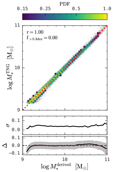
Figure 1: Comparison of estimated stellar mass using our method against actual values in TNG100. Individual galaxies are represented by gray dots, and the heatmap illustrates the normalized probability distribution. The one-to-one reference line is shown in a red dashed line. Spearman’s rank correlation coefficient ($r$) and the fraction of outliers ($f_{\rm>0.3dex}$) are presented in the top left corner. The lower two panels show the standard deviation and the systematic bias as a function of estimated stellar mass. The grey-shaded region in the bottom panel shows the median uncertainty. This figure demonstrates our method’s accuracy ($\approx 0.05$ dex) and negligible systematic bias in estimating stellar masses from broad-band optical photometry.

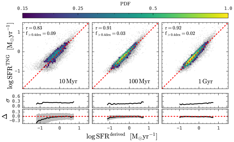
Figure 2: Similar to Fig. 1, this figure displays the estimation accuracy of SFRs over three timescales: 10Myr (left), 100Myr (middle), and 1Gyr (right). Gray dots represent individual star-forming galaxies in TNG100, and the heatmap illustrates the normalized probability distribution. This figure demonstrates our method’s effectiveness in recovering SFR with an accuracy of $\lesssim 0.3$ dex and negligible systematic bias.

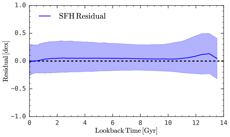
Figure 3: The distribution of SFH residuals (derived SFHs minus real SFHs in TNG100). The blue solid line shows the median residual, with the blue-shaded region denoting a 1-sigma distribution. This figure illustrates our method’s capability to estimate galaxy SFHs with about 0.1 dex error for the median and 0.3 dex error when considering the 1-sigma distribution.

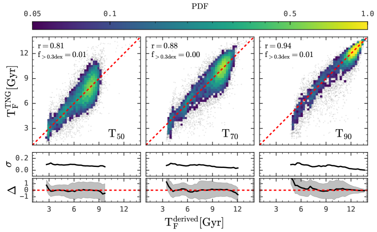
Figure 4: Similar to Fig. 1, this figure extends the analysis to the lookback time when 50% (left), 70% (middle), and 90% (right) of the stellar population has formed. Individual gray dots represent galaxies in TNG100, and the heatmap illustrates the normalized probability distribution. This figure illustrates our method’s capability to estimate typical galaxy formation times with a fractional standard deviation of around 30% and negligible systematic bias.

We first test the performance of our method on the simulated galaxies in the IllustrisTNG simulation before we apply it to the observational galaxy sample. For each simulated galaxy, it is possible to obtain its SFH, metal enrichment history, and stellar mass-to-light ratio from the stellar particles it contains. We then apply a self-consistency test with all other simulated galaxies as priors to estimate these properties for the $i$-th galaxy. The accuracy of our method was quantified by comparing these estimates to the properties derived directly from the galaxies’ stellar particles.

We first estimate the r-band mass-to-light ratio and derive the stellar mass. The results, shown in Fig. 1, indicate that our method reliably estimates stellar masses, with the majority of galaxies exhibiting less than 0.3 dex deviation from their true values, and a scatter of less than 0.05 dex. We also test another approach based on z-band mass-to-light ratio, which provides similar results.

Similarly, Fig. 2 illustrates the method’s robustness in accurately estimating the SFRs averaged over three different time scales, which correspond to different observation probes: 10Myr for indicators based on the $\rm H\alpha$ emission, 100Myr for indicators based on the UV luminosity or IR and FIR luminosities, and 1Gyr for indicators based on $\rm D_{n}(4000)$ index. Note that we only present the SFR estimates for galaxies that are classified as star-forming, defined as those with $\log\mathrm{SFR}>\log M_{*}\times 0.76-8.1$ (above the red dashed line in the right panels of Fig. 7). This threshold is derived by shifting the best-fit star-forming main sequence from Renzini & Peng (2015) downward by approximately 0.5 dex. Here one can see that the standard deviation is about $0.3$ dex for the SFR smoothed on these three timescales. Notably, the resolution limit of TNG100 ($\sim 10^{6}\rm M_{\odot}$ for baryonic mass) suggests a minimally detectable SFR of approximately $0.1\rm M_{\odot}/yr$ over a 10Myr time scale for particle-based methods.

Finally, Fig. 3 and Fig. 4 show the comparison of star formation histories. The SFHs are parametrized with the method described in Appendix A. From the SFH residual shown in Fig. 3, the SFHs of individual galaxies can be recovered within 0.1 dex when the median is considered, and within 0.3 dex error when 1-sigma distribution is considered. Here we also represent the SFH with the cosmic time that a certain fraction ($50\%$, $70\%$, and $90\%$) of stars have formed in Fig. 4. Again, it is evident that our method can recover the SFH for individual galaxies quite well with scatter below $\sim 0.2$ dex.

5 The application to SDSS

Following successful validation on the IllustrisTNG simulation, we apply our method to the SDSS main galaxy sample to infer stellar mass, current SFR, and SFH from broad-band photometry, utilizing the TNG100 galaxies as templates for mass-to-light ratio, SFH, and metal enrichment history.

5.1 Stellar mass and SFR

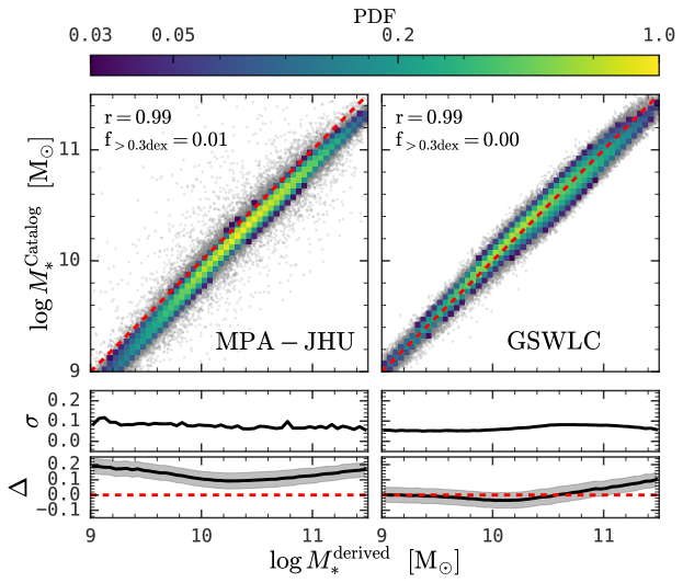
Figure 5: The top panels show the comparison of the stellar mass estimated by our method versus those in MPA-JHU (left; Kauffmann et al., 2003) and GSWLC (right; Salim et al., 2016). Individual galaxies in SDSS are represented by gray dots, and the heatmap illustrates the normalized probability distribution. The bottom panels show the standard deviations and mean differences as functions of estimated stellar mass. Our method aligns closely with GSWLC values and consistently shows an approximate 0.13 dex systematic increase over MPA-JHU estimates.

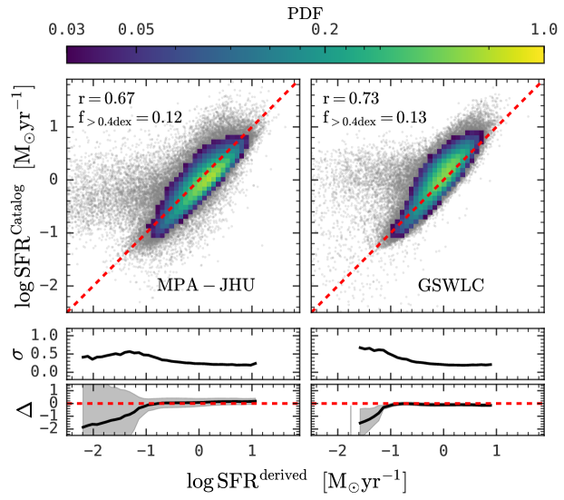
Figure 6: Similar to Fig. 5, focusing on the SFR for star-forming galaxies. Individual star-forming SDSS galaxies are represented by gray dots, and the heatmap illustrates the normalized probability distribution. Our estimates align well with MPA-JHU and GSWLC values above $0.1\rm M_{\odot}yr^{-1}$.

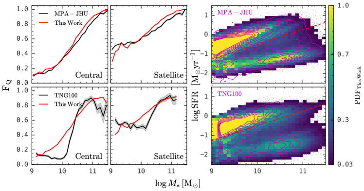
Figure 7: The left four panels show quiescent galaxies fraction as a function of stellar mass for central (left) and satellite (right) galaxies. The red solid lines are our estimates smoothed on 10 Myr (top) and 100 Myr (bottom), in comparison with the results from the MPA-JHU catalog (top) and the TNG100 simulation (bottom). The right two panels show the distribution of galaxies on the $\log M_{*}\rm-\log SFR$ plane. Individual galaxies are represented by gray dots, and the heatmap illustrates the normalized probability distribution. The red dashed line ($\log\mathrm{SFR}=0.76\times\log M_{*}-8.1$) separates the star-forming and quiescent galaxies. The magenta solid contour lines are for our results with the SFR smoothed on 10 Myr (top) and 100 Myr (bottom), and the color maps are for the MPA-JHU result and the TNG100 simulation, respectively. Our method’s results closely match the MPA-JHU observations in bi-modality and show distinct deviations from TNG100 predictions, reinforcing the effectiveness of using TNG100 as a prior without replicating simulation biases.

Fig. 5 shows the stellar mass recovered with our method in comparison with values in the MPA-JHU and GSWLC catalog. Note that the MPA-JHU catalog derives stellar mass from the spectral indices for the central part covered by the fiber and from the broad-band photometry for the outer part. Our result agrees with that of the MPA-JHU with the standard deviation $\lesssim 0.1$ dex, except that our stellar mass is systematically larger than theirs by about 0.13 dex. Note that we already corrected the difference caused by the initial mass function and cosmology. Such systematical difference is also reported by Salim et al. (2016), where they attribute it to the different parametric function forms for the SFH. From the right panels of Fig. 5, one can see that our result agrees with the GSWLC catalog (Salim et al., 2016) quite well with a standard deviation $\lesssim 0.1$ dex and negligible systematics, which suggests that the stellar mass in MPA-JHU is indeed biased by their non-physical priors of SFH. Moreover, it is noteworthy that the GSWLC catalog derives the stellar mass from the UV to the IR photometry, while we only use five optical broad-band photometry.

Fig. 6 shows the comparison of SFR for star-forming galaxies between our estimation and that of the MPA-JHU and GSWLC catalog. For this figure, the star-forming galaxies are selected following the color-magnitude diagram criteria from Baldry et al. (2004) since there is no real SFR in observation. We also test the results with different criteria, including the color-stellar mass diagram (Cui et al., 2024) and stellar mass - SFR diagram ($\log\mathrm{SFR}>\log M_{*}\times 0.76-0.81$, galaxies above the red dashed line in the upper right panel of Fig. 7). There are no noticeable changes among these different definitions. For passive galaxies, their SFRs in MPA-JHU and GSWLC have high uncertainties (Salim et al., 2016) and may even be upper limits, possibly due to the inaccurate photometry for GSWLC (Li et al., 2023) and uncertainty in the $\rm D_{n}4000-sSFR$ relation (Brinchmann et al., 2004). So these passive galaxies are not considered for comparison. Note that the star formation rate in the MPA-JHU catalog is calibrated with the $\rm H\alpha$ luminosity, which traces the star formation activity in the last 10Myr, and that of GSWLC is estimated by smoothing the inferred SFH on 100Myr. Thus, we choose to take the averaged SFR over 10Myr and 100Myr for a fair comparison with each catalog. Here one can see that, for galaxies with ${\rm SFR}>0.1\rm M_{\odot}/yr$, our method produces consistent results with MPA-JHU and GSWLC with the standard deviation about $0.2-0.5$ dex and negligible systematics. Finally, it should be emphasized that the GSWLC catalog uses additional information from the UV and IR emissions and MPA-JHU uses the $\rm H\alpha$ emission and $\rm D_{n}(4000)$ spectral index, while our method only uses five optical broad-band photometry. Still, we yield consistent results, indicating the superiority of our method.

We note that for some galaxies, our model systematically provides lower SFR estimates than those from MPA-JHU and GSWLC. Although the true SFRs are unknown, these galaxies are all classified as star-forming; therefore, the measurements from MPA-JHU and GSWLC, which utilize $\rm H\alpha$ emission and UV plus IR photometry respectively, should theoretically be more accurate. It is also interesting to note that this discrepancy is almost non-existent in the self-consistency test (Fig. 2), suggesting that the issue likely does not originate from the link between SEDs and SFH or our method itself. One possible explanation is the insufficient sampling of SFH space in the simulation. However, this problem does not significantly impact the results statistically, as the catastrophic failure rate is low (approximately 20%).

Before we step into the comparison of quiescent fraction and SFR bi-modality, several technical considerations should be mentioned. Firstly, we choose to compare with the MPA-JHU catalog rather than the GSWLC catalog, since the latter suffers from incompleteness due to the requirement of cross-matching with the UV and IR photometry catalog. Secondly, we note that TNG100 produces many quiescent galaxies with SFR equal to zero, which is not suitable for presentation, so we assign some small SFR to these galaxies for the sake of fair comparison with observational results. It is noteworthy that some work argues that the distribution of galaxies on the $\log M_{*}\rm-\log SFR$ plane is unimodal: a star-forming peak and an extended tail towards low SFR (see Renzini & Peng, 2015; Feldmann, 2017; Eales et al., 2017). Thirdly, the calculation of SFR from the amount of stellar particles formed in the last period suffers from the shot noise. We note that the baryon cell weighs about $10^{6}\rm M_{\odot}$ in TNG100, so the minimal SFR above zero in the last 10Myr will be $0.1\rm M_{\odot}/yr$, which corresponds to a specific SFR of $10^{-10}\rm yr^{-1}$ for a $10^{9}\rm M_{\odot}$ galaxy and, hence, it will affect the calculation of quiescent fraction. Therefore, we choose to smooth the SFR over 100Myr to minimize this effect when we compare our results with TNG100.

Fig. 7 shows the quiescent fraction for central and satellite galaxies, respectively, and the apparent bimodal distribution of galaxies on the $\log M_{*}\rm-\log SFR$ plane. Here we employ the group catalog in Yang et al. (2007) to classify central and satellite galaxies. Firstly, the quiescent fraction for central galaxies monotonically increases with stellar mass from about 10% at $10^{9}\rm M_{\odot}$ to almost 100% at $10^{11.5}\rm M_{\odot}$, which is a manifestation of mass quenching. As reported in Wang et al. (2023), a large portion of low- mass quiescent central galaxies are backsplash galaxies, which were previously satellite galaxies of other massive halos and got ejected out of their host halos. Secondly, the quiescent fraction of the central galaxies in TNG100 abruptly increase around $10^{10.2}\rm M_{\odot}$, which is absent in observational data. The sharp transition may result from the problematic AGN feedback interpretation in TNG (see Terrazas et al., 2020, for more information). In addition, the result obtained from our method is consistent with MPA-JHU and previous results (Baldry et al., 2006; Peng et al., 2010, 2012; Wetzel et al., 2013; Trussler et al., 2020; Gallazzi et al., 2021) while significantly differing from the TNG100 simulation, thus confirming the robustness of our approach in applying physical priors without duplicating simulation results. Thirdly, satellite galaxies are more quenched than central galaxies at a given stellar mass, since they are additionally subject to environmental effects. Finally, we found three components in the distribution of galaxies on the $\log M_{*}\rm-\log SFR$ plane: one star-forming main sequence, one massive quiescent component contributed by mass quenching, and one low-mass quiescent component from environmental quenching (see Renzini & Peng, 2015). One notable thing is that we can accurately reproduce the star-forming main sequence exhibited in the MPA-JHU catalog, which is derived from $\rm H\alpha$ luminosity, while our results are only based on five broad-band photometry.

5.2 Cosmic SFR density and stellar mass density

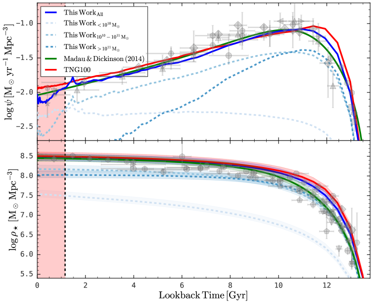
Figure 8: The upper panel depict the comparison of the cosmic SFR density, defined as the comoving SFR density as a function of lookback time. The gray symbols are the observational results from direct SFR density estimates at different redshifts (Sanders et al., 2003; Takeuchi et al., 2003; Wyder et al., 2005; Schiminovich et al., 2005; Dahlen et al., 2007; Reddy & Steidel, 2009; Robotham & Driver, 2011; Magnelli et al., 2011; Cucciati et al., 2012; Bouwens et al., 2012a, b; Schenker et al., 2013; Magnelli et al., 2013; Gruppioni et al., 2013; Madau & Dickinson, 2014), and the fitting line of these observational results are shown in green solid line (Madau & Dickinson, 2014). The result of the TNG100 simulation is shown in the red solid line and the result obtained with our method is shown in the blue solid line. The three blue dashed lines are the cosmic SFR density that end up in descendant galaxies with different stellar masses at $z\sim 0$. The lower panel shows the comparison of the cosmic stellar mass density, defined as the comoving stellar mass density as a function of lookback time. Solid lines are integrated from cosmic SFR density with a return factor of 0.41 (based on the Chabrier IMF). The error bands are based on return factors of 0.25 and 0.5. The gray symbols are the observational results integrated from stellar mass functions between $\rm 10^{8}M_{\odot}$ and $\rm 10^{13}M_{\odot}$ (Caputi et al., 2011; González et al., 2011; Santini et al., 2012; Ilbert et al., 2013; Muzzin et al., 2013; Duncan et al., 2014; Grazian et al., 2015; Caputi et al., 2015; Wright et al., 2018; Kikuchihara et al., 2020; McLeod et al., 2021; Thorne et al., 2021; Weaver et al., 2023). Our method effectively captures both the cosmic SFR density and cosmic stellar mass density, aligning closely with direct measurements and revealing detailed insights into galaxy evolution.

As demonstrated in § 3 and tested in § 4, our method is able to recover the star formation history of each galaxy from their broad-band photometry. By doing so for all galaxies in the SDSS main galaxy sample, the cosmic SFR density, i.e., the comoving SFR density as a function of redshift, can be recovered by aggregating individual SFHs of local galaxies and dividing it with the comoving volume occupied by these galaxies. This is known as the fossil record method and has been applied in many works (Heavens et al., 2004; Gallazzi et al., 2008; Madau & Dickinson, 2014; Carnall et al., 2019; Leja et al., 2019; Sánchez et al., 2019), which should have similar results to direct observation (Lilly et al., 1996; Madau et al., 1996) in principle. It is noteworthy that, since SDSS is a flux-limited sample, the comoving volume occupied by observed galaxies is dependent on the intrinsic luminosity, which is commonly refer to as $V_{\rm max}$ (Schmidt, 1968).

The top panel of Fig. 8 shows the cosmic SFR density reconstructed from the individual 100 bins SFH of local galaxies in blue solid line. For comparison, we also present the result from TNG100 in red solid line, the direct observational measurement results in gray symbols with the fitting function in green solid line (Sanders et al., 2003; Takeuchi et al., 2003; Wyder et al., 2005; Schiminovich et al., 2005; Dahlen et al., 2007; Reddy & Steidel, 2009; Robotham & Driver, 2011; Magnelli et al., 2011; Cucciati et al., 2012; Bouwens et al., 2012a, b; Schenker et al., 2013; Magnelli et al., 2013; Gruppioni et al., 2013; Madau & Dickinson, 2014). Here one can see that TNG100 slightly over-predicts the peak position by $\approx 1\rm Gyr$, while our method, although using TNG100 as a prior, is a better match to the observational result from direct measurements. It is noteworthy that our method outperforms several previous parametric and non-parametric SFH methods (see Carnall et al., 2019; Leja et al., 2019), which confirms the superiority of our method in delivering physical parameters from the multi-band photometry.

The three dashed lines in the top panel of Fig. 8 show the cosmic star formation histories contributed by $z\sim 0$ descendant galaxies with different stellar masses. For massive galaxies, although their assembly is relatively recent, most of their stars were already formed more than 10 Gyrs ago, which is known as the archaeology downsizing effect (Thomas et al., 2005; Nelan et al., 2005; Heavens et al., 2004; Jimenez et al., 2005; Neistein et al., 2006; Renzini, 2006). Meanwhile, stars formed in recent several Gyrs end up in low mass galaxies, which is expected since massive galaxies are quenched and stop producing new stars (see Fig. 7).

By integrating the cosmic SFR density and assuming a return factor of 0.41 from the Chabrier initial mass function, we also derive the cosmic stellar mass density in the bottom panel of Fig. 8. The results from TNG100 and (Madau & Dickinson, 2014) and TNG100 are also shown in green and red for comparison. Gray symbols are cosmic stellar mass density integrated from stellar mass function in the literature (Caputi et al., 2011; González et al., 2011; Santini et al., 2012; Ilbert et al., 2013; Muzzin et al., 2013; Duncan et al., 2014; Grazian et al., 2015; Caputi et al., 2015; Wright et al., 2018; Kikuchihara et al., 2020; McLeod et al., 2021; Thorne et al., 2021; Weaver et al., 2023). Our results agree with both (Madau & Dickinson, 2014) and stellar mass function results well, while TNG100 slightly exceeds most measurements about 10 Gyr ago. When categorizing galaxies into descendant stellar mass bins, we again see the archaeology downsizing effect: massive galaxies form their mass early and gradually cease star formation. In contrast, low-mass galaxies keep on creating new stars.

5.3 Reconstructing spectral indices

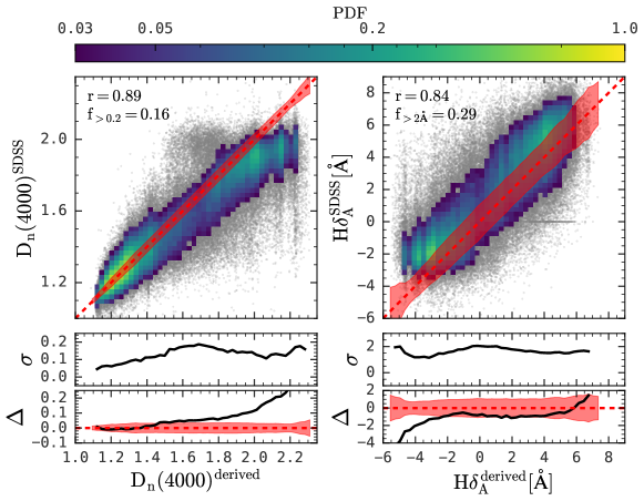
Figure 9: The top panels show the comparison between measured and reconstructed spectral indices, $\rm D_{n}(4000)$ (left) and $\rm H\delta_{A}$ (right) for the SDSS main galaxy sample. Individual galaxies are represented by gray dots, and the heatmap illustrates the normalized probability distribution. The bottom panels highlight the standard deviation and systematic bias relative to directly measured values. The red-shaded regions show the median observational errors. This figure shows that our reconstructed spectral indices resemble the directly measured values with strong correlations (Spearman’s coefficient $\approx 0.85$)

Previous studies found that the spectral indices of observed galaxies contain abundant information about the physical properties of galaxies, and these spectral indices are used to derive physical properties, such as stellar mass, SFH and stellar metallicity (Faber, 1972; Worthey & Ottaviani, 1997; Kauffmann et al., 2003; Gallazzi et al., 2005), and are incorporated into the full-spectrum fitting procedure to deliver more accurate property estimations. Thus, given the success of our method based on broad-band photometry, it is pertinent to investigate the extent to which the spectral indices of observed galaxies can be reconstructed. Here we focus on $\rm D_{n}(4000)$ and $\rm H\delta_{A}$. Here $\rm D_{n}(4000)$ quantifies the discontinuity around 4000Å, which comes from the absorption of ionized metals, and it is defined as the ratio of the average flux density in the band 3850-3950 and 4000-4100Å  (see Balogh et al., 1999; Kauffmann et al., 2003). $\rm D_{n}(4000)$ is profoundly dependent on the stellar age and stellar metallicity: older and more metal-rich galaxies exhibit higher $\rm D_{n}(4000)$. Particularly, $\rm D_{n}(4000)$ is sensitive to the median stellar age. $\rm H\delta_{A}$ quantifies the $\rm H\delta$ absorption lines (Worthey & Ottaviani, 1997), which are mainly contributed by late-B and early-F stars, and therefore, $\rm H\delta_{A}$ is a sensitive probe of star formation activities that occurred 0.1-1Gyr ago (Kauffmann et al., 2004). Notice that the $\rm D_{n}(4000)$ and $\rm H\delta_{A}$ distributions of TNG100 galaxies are similar to observation (Wu et al., 2018, 2021), indicating the SFH distribution in TNG is generally accurate. It is noteworthy that both spectral indices are not significantly affected by the presence of dust absorption (Kauffmann et al., 2003; MacArthur, 2005, also see the test in Appendix C), allowing for the safe exclusion of this effect in the forward synthesis of these two spectral indices.

Here is the procedure to reconstruct the spectral indices ($\rm D_{n}(4000)$ and $\rm H\delta_{A}$) from the broad-band photometry of observed SDSS galaxies. Firstly, we derive the SFH and the metal enrichment history of each observed galaxy from its broad-band photometry using our method (see § 3) with TNG100 as a physical prior. Secondly, we synthesize the full spectrum of each galaxy from its SFH and metal enrichment history using the fsps package adopting MILES stellar library, Padova isochrones, and Chabrier IMF. Finally, we measure the spectral indices following the procedure done for the observed spectrum.

Fig. 9 shows the comparison between the reconstructed and the observed spectral indices. It should be noted that we exclude galaxies with unreliable spectral index measurements, which includes galaxies whose measurement error in $\rm D_{n}(4000)$ is above 0.07 or whose measurement error in $\rm H\delta_{A}$ is above 2.5Å. This excludes 5% and 4% of SDSS galaxies, respectively. Here one can see that Spearman’s correlation coefficients for both indices are around 0.85, which means that about 85% of the variation for these two spectral indices can be captured by the optical broad-band photometry. Besides, the reconstructed spectral indices closely follow the observed values on the one-to-one line except for galaxies with high $\rm D_{n}(4000)$ and negative $\rm H\delta_{A}$, which are quenched galaxies and dominated by old stellar populations. We have inspected the result for star-forming galaxies (not shown here) and found that the systematic deviation becomes negligible.

Many previous studies have conducted similar tests on different SED fitting procedures. For instance, Chen et al. (2012) developed a method based on principal component analysis (PCA) and applied it to BOSS spectra. They were able to retrieve the $\rm D_{n}(4000)$ and $\rm H\delta_{A}$ indices for high redshift galaxies ($0.4<z<0.7$) with a precision comparable to our model, benefiting from the rich information available in the full spectra. In a related study, Nersesian et al. (2024) utilized the Prospector procedure on galaxies around $z\sim 1$ with the COSMOS2020 photometry. Their results, which involved comparisons with direct observations from the Large Early Galaxy Astrophysics Census (LEGA-C) survey (van der Wel et al., 2016, 2021), demonstrated that the recovered $\rm H\delta_{A}$ indices generally aligned with actual measurements, showing no significant systematic offsets. These findings are consistent with our results.

The success in reconstructing spectral indices has three implications. Firstly, our method can deliver physical SFHs and metal enrichment histories, so that the synthesized spectral indices resemble the results obtained from direct observation, even though we only use broad-band photometry. Secondly, much information provided by these two spectral indices is contained in broad-band photometry. Thirdly, the remaining $\approx 15\%$ variation contains additional information about the underlying interesting physical properties (Nersesian et al., 2024), whose extraction requires an extension of the current method to the full-spectrum situation. This could be explored in future work.

6 Summary

The spectral energy distributions (SEDs) of galaxies contain rich information about their evolutionary histories and have been routinely used to derive fundamental galaxy properties such as stellar mass, SFR, stellar age, and star formation history (SFH) through SED fitting techniques. However, SED fitting, especially when limited to broad-band photometry, may not be sufficient to tightly constrain the SFH and metal enrichment history. Consequently, conventional methods, both parametric and non-parametric, often fail to accurately recover the observed cosmic SFR density, due to strong degeneracy, and oversimplified and non-physical assumptions about SFHs that are unable to account for complex SFH variations across different galaxy populations.

To address this issue, this study introduces a novel method for estimating the physical properties of galaxies from their observed broad-band SEDs, utilizing hydrodynamical galaxy formation simulations as priors. We validated this method on simulated galaxies and subsequently applied it to observations. Our main findings are summarized as follows:

1. Testing on the TNG100 SDSS-mock with five-band photometry ($u,g,r,i,z$) including dust effects, our method accurately recovers the stellar mass, current SFR, and typical galaxy formation times from optical broad-band photometry. The standard deviations are around 0.05, 0.3, and 0.2 dex, respectively, and the systematic bias is negligible (see Fig. 1, 2, and 4).

2. When applied to observed SDSS galaxies using optical photometry ($u,g,r,i,z$) with spectroscopic redshift, our method consistently estimates stellar mass and SFRs that align with those in the MPA-JHU and GSWLC catalogs, showing a standard deviation of $\sim 0.1$ dex for stellar mass and $\sim 0.4$ dex for SFR (see Fig. 5 and 6).

3. Using the derived stellar mass and SFR from our method on a mass-completed sample in SDSS, the bimodal distribution of galaxies on the $\log M_{*}\rm-\log SFR$ plane (i.e., main sequence and passive sequence) and the quenched fraction for centrals and satellites all closely match those obtained from MPA-JHU results. Interestingly, despite employing SFHs from TNG100 as priors, the statistical properties of derived galaxy properties (such as the main sequence, quenched fraction, and environmental effects) are more aligned with MPA-JHU than TNG itself (see Fig. 7). For instance, the sharp quenching threshold around $\log M_{*}\sim 10.5$ in TNG100 (as shown in Fig. 7) is due to its implemented active galactic nucleus (AGN) feedback model. The quenched fractions derived from our method evidently have not been influenced by these specific quenching mechanisms in TNG.

4. Using the SFHs of individual SDSS galaxies derived from our method, we estimate the cosmic SFR density, and also the cosmic stellar mass density by integrating these SFHs. Both results show remarkable consistency with direct observational measurements up to $z\sim 6$. This is the first time that SFHs derived from SEDs accurately match direct observational measurements. We also find that the stellar populations of massive galaxies are already largely formed about 10 Gyrs ago, while recent star formation predominantly occurs in low-mass galaxies (see Fig. 8), consistent with the downsizing trend established in the literature.

5. From the estimated SFHs and metal enrichment histories of individual galaxies in SDSS, we synthesise two spectral indices, $\rm D_{n}(4000)$ and $\rm H\delta_{A}$. Our synthesized spectral indices closely match direct observational results. This validation supports the reliability of our derived star formation and metal enrichment histories, despite solely relying on broad-band photometry (see Fig. 9).

It is important to note that our method does not depend on simulations being considered “the truth” (e.g. TNG100). Unlike conventional parametric methods, simulations offer a large set of physically realistic SFH templates. As a result, our approach effectively excludes many physically unrealistic SFHs that are often included in conventional SED fitting methods, which might otherwise yield better fits due to strong degeneracies within the SED. This exclusion of physically unrealistic templates represents a significant advantage of our methodology.

Meanwhile, we must also emphasize that galaxies in the real universe may or may not follow every SFH provided by the simulations. And the relative fraction of certain galaxy populations that evolve according to a specific SFH may differ significantly from those predicted by the simulations. In fact, when applying our method to SDSS galaxies, as illustrated in Fig. 7, we successfully recovered the observed quench fraction and the detailed distribution of galaxies on the $\log M_{*}\rm-\log SFR$ plane, whereas TNG100 produced noticeably different results. The derived star formation rate density and stellar mass density from our method also show a better match with direct observations compared to TNG100.

Our method not only provides robust and accurate estimates of stellar population evolution, particularly galaxy SFHs, using only broad-band photometry but also demonstrates high efficiency. Our tests show that it can process the star formation and metal enrichment histories for one million galaxies in less than ten minutes using a single Intel-i5 core. These features make it an exceptionally promising tool for ongoing facilities like Euclid (Laureijs et al., 2011) and upcoming ones such as the CSST (Chinese Space Station Telescope, Zhan, 2011) and LSST (Large Synoptic Survey Telescope, Ivezić et al., 2019), which will deliver vast quantities of high-quality multi-band photometric data. Moreover, its outstanding computational efficiency allows for the application of pixel-to-pixel SED fittings to derive the resolved galaxy properties. In the future, we will use this method also for galaxy samples at high redshifts, using TNG templates at the corresponding cosmic times.

Data availability

The data underlying this article will be shared on reasonable request to the corresponding author.

Appendix A Parameterization of SFH

This appendix discusses our method for parameterizing SFHs of galaxies within the IllustrisTNG framework. Instead of relying solely on discrete snapshots, our approach integrates the formation times and initial masses of stellar particles over continuous periods to accurately reflect the galaxy’s current spectral energy distribution. This method accounts for the dynamic changes in stellar particle locations due to processes such as mergers and interactions.

We adopt a refined SFH binning algorithm adapted from Shamshiri et al. (2015), where we set the nearest bin to the present epoch ($z=0$) at $t_{0}=0.01$ Gyr. The bins increase exponentially back in time:

$$b^{0}t_{0},\,b^{0}t_{0},\,b^{1}t_{0},\,b^{1}t_{0},\,...,\,b^{n}t_{0},\,b^{n}t_{0}$$ (A1)

where $b$ is the scaling factor and $2(n+1)$ the total number of bins. The age of the universe, $T$, is thus:

$$T=\sum_{i=0}^{n}2b^{i}t_{0}=2\frac{b^{n+1}-1}{b-1}t_{0}$$ (A2)

Determining the values for $t_{0}$, $2(n+1)$, and $b$ allows us to define the time intervals for each bin accurately. We conduct a test to evaluate the efficacy of this algorithm in recovering the actual spectra of galaxies and to determine the optimal number of bins required for reconstruction. For this test, we perform a stellar population analysis on galaxies in TNG100 simulation using fsps and compare the spectra generated with different binning algorithms and bin numbers. Since our objective is to test the SFH, we only consider the continuum from the stellar component.

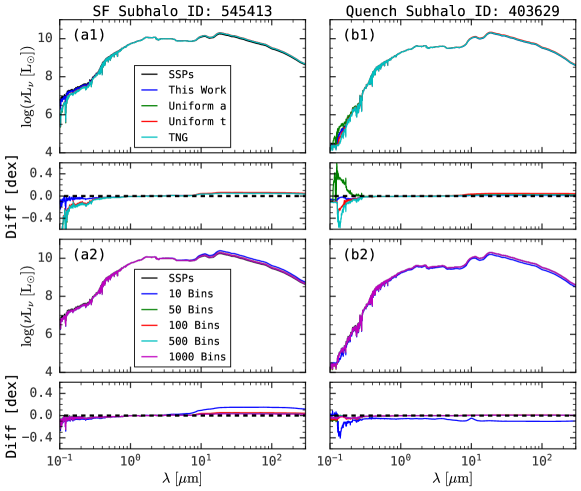
Figure 10: Spectra generated with fsps using various SFH binning algorithms and bin numbers are compared. Both star-forming and quenched galaxies are included, with Subhalo IDs 545413 and 403629, from left to right respectively. The spectra discrepancies between different methods and real spectra generated by combining stellar particles as single stellar populations are quantified in dex in the lower panels. The top two figures (a1, b1) present the comparison between different SFH binning algorithms with a fixed number of 100 bins. The blue lines correspond to spectra with the SFH binning algorithm employed in this study. The green and red lines represent spectra generated using uniform scale factors and a uniform time SFH binning algorithm, respectively. The cyan lines demonstrate the binning method that utilizes TNG snapshots as bin edges. The bottom figures (a2, b2) display the spectra with varying bin numbers using our method, ranging from 10 bins to 1000 bins. This figure illustrates that our method, utilizing 100 bins, effectively recovers UV to IR spectra with minimal bias (less than 0.1 dex).

As shown in Figure 10, we evaluate the SFH binning algorithms by comparing their ability to reconstruct the real spectra of a star-forming galaxy (Subhalo ID = 545413) and a quenched galaxy (Subhalo ID = 403629). The effectiveness of each method is measured by the accuracy with which it captures the spectral details

We first treat each stellar particle in the galaxy as a single stellar population and combine them to obtain the most accurate real spectra. We then evaluate different SFH binning methods in the upper panels of Figure 10(a1) and (b1) with 100 bins, including methods used in this study, bins with uniform scale factor a, and uniform time intervals. We also utilize TNG snapshots as bin edges (and add another bin edge at scale factor a = 0). Galaxies are then expressed as 100 single stellar populations formed in the middle of the bin.

For most galaxies, our SFH binning algorithm can recover the real spectra within 0.1 dex, while other binning methods can lead to significant bias to the real spectra in the short wavelength range. This is because our method can provide a much smaller bin size near z=0, where recent star formation can contribute significantly to UV spectra. We also investigate the influence of bin numbers for our method in Figure 10 (a2) and (b2), with bin numbers ranging from 10 to 1000. Our analysis confirms that using 100 bins optimally balances computational efficiency and the fidelity of spectral recovery within 0.1 dex. The results validate our algorithm’s capability to reconstruct detailed and accurate SFHs for galaxies, supporting its application in broader astrophysical studies.

Appendix B Validation of SFH-based Cosmic SFR Density

This appendix assesses the accuracy of deriving cosmic SFR density using the SFHs of galaxies (the fossil record method) from the IllustrisTNG simulation compared to direct snapshot-based methods.

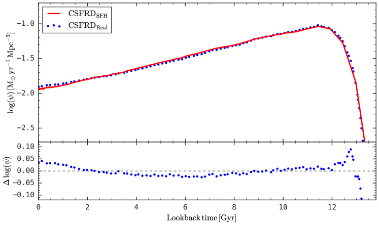
Figure 11: Comparison between SFH-based and direct measurement of cosmic SFR density in TNG100: In the upper panel, the red line shows the cosmic SFR density calculated as the sum of the SFHs of all TNG100 galaxies with a stellar mass more than $10^{9}\,h^{-1}\,\mathrm{M}_{\odot}$ at z=0, while the blue dots depict the direct measurements of SFRs from galaxies in each TNG100 snapshot. Differences are highlighted in the lower panel, showing minor discrepancies (less than 0.05 dex).

Cosmic SFR density is traditionally estimated from IR and UV luminosity functions representing direct observations across various epochs. The SFH-based approach applied in this work, aggregating historical star formation data from simulations, provides an alternative estimation method. The latter approach gives a smaller value than the former because of the contribution of intra-cluster light and small galaxies. Here we quantify the difference between these two approaches using TNG100 in Figure 11.

The upper panel shows the SFH-based SFR density (red line) against the directly measured ones from TNG100 snapshots (blue dots). The lower panel illustrates their differences, predominantly less than 0.05 dex, suggesting that our SFH-based method captures the cosmic SFR density with minimal bias, despite minor deviations in early epochs due to coarse temporal resolution in SFH sampling. This supports the robustness of using integrated SFH for cosmic SFR density estimation in cosmological studies.

Appendix C Evaluating Dust Attenuation on Spectral Indices

In this appendix, we investigate the effects of dust attenuation on spectral indices, which were not considered in our initial stellar population synthesis. We assess how dust impacts the indices $\rm D_{n}(4000)$ and $\rm H\delta_{A}$, which are critical for interpreting the age and activity of stellar populations.

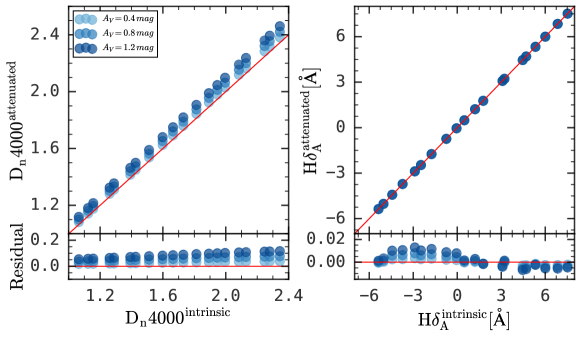
Figure 12: Impact of Dust Attenuation on Spectral Indices $\rm D_{n}(4000)$ and $\rm H\delta_{A}$: The upper panels compare intrinsic and dust-affected indices across 20 randomly selected TNG100 galaxies. Galaxies with different $A_{V}$ are indicated by different colors. The red solid lines are the one-to-one reference lines. The lower panels quantify the differences. These two spectral indices are insensitive to dust attenuation, with the largest changes being $\lesssim 0.15$ for $\rm D_{n}(4000)$ and $\lesssim 0.02$Å for $\rm H\delta_{A}$.

Using fsps, we generate mock spectra for a representative sample of TNG100 galaxies and apply the extinction law from Calzetti et al. (2000) to simulate dust effects. This process involves varying levels of attenuation ($A_{V}=0.4,0.8,1.2$ mag) to cover a broad range of realistic conditions (See Fig.8b in Salim & Narayanan, 2020). Our findings in Fig 12 confirm that both $\rm D_{n}(4000)$ and $\rm H\delta_{A}$ are relatively robust against dust, with only minor deviations observed even under significant dust presence. For $\rm D_{n}4000$, attenuation raises the value and this effect becomes stronger for higher intrinsic $\rm D_{n}4000$ galaxies. For $\rm H\delta_{A}$, there seems no clear trend. This reinforces the utility of these indices in dusty environments and aligns with findings from prior studies, such as those by Kauffmann et al. (2003), highlighting their reliability in diverse galactic conditions.

References

- Abazajian et al. (2009) Abazajian, K. N., Adelman-McCarthy, J. K., Agüeros, M. A., et al. 2009, ApJS, 182, 543, doi: 10.1088/0067-0049/182/2/543
- Abramson et al. (2016) Abramson, L. E., Gladders, M. D., Dressler, A., et al. 2016, ApJ, 832, 7, doi: 10.3847/0004-637X/832/1/7
- Astropy Collaboration et al. (2022) Astropy Collaboration, Price-Whelan, A. M., Lim, P. L., et al. 2022, ApJ, 935, 167, doi: 10.3847/1538-4357/ac7c74
- Baldry et al. (2006) Baldry, I. K., Balogh, M. L., Bower, R. G., et al. 2006, MNRAS, 373, 469, doi: 10.1111/j.1365-2966.2006.11081.x
- Baldry et al. (2004) Baldry, I. K., Glazebrook, K., Brinkmann, J., et al. 2004, ApJ, 600, 681, doi: 10.1086/380092
- Balogh et al. (1999) Balogh, M. L., Morris, S. L., Yee, H. K. C., Carlberg, R. G., & Ellingson, E. 1999, ApJ, 527, 54, doi: 10.1086/308056
- Barbary (2016) Barbary, K. 2016, extinction v0.3.0, Zenodo, doi: 10.5281/zenodo.804967
- Behroozi et al. (2019) Behroozi, P., Wechsler, R. H., Hearin, A. P., & Conroy, C. 2019, MNRAS, 488, 3143, doi: 10.1093/mnras/stz1182
- Blanton & Roweis (2007) Blanton, M. R., & Roweis, S. 2007, AJ, 133, 734, doi: 10.1086/510127
- Blanton et al. (2005) Blanton, M. R., Schlegel, D. J., Strauss, M. A., et al. 2005, AJ, 129, 2562, doi: 10.1086/429803
- Boquien et al. (2019) Boquien, M., Burgarella, D., Roehlly, Y., et al. 2019, A&A, 622, A103, doi: 10.1051/0004-6361/201834156
- Bouché et al. (2010) Bouché, N., Dekel, A., Genzel, R., et al. 2010, ApJ, 718, 1001, doi: 10.1088/0004-637X/718/2/1001
- Bouwens et al. (2012a) Bouwens, R. J., Illingworth, G. D., Oesch, P. A., et al. 2012a, ApJ, 754, 83, doi: 10.1088/0004-637X/754/2/83
- Bouwens et al. (2012b) —. 2012b, ApJ, 752, L5, doi: 10.1088/2041-8205/752/1/L5
- Brinchmann et al. (2004) Brinchmann, J., Charlot, S., White, S. D. M., et al. 2004, MNRAS, 351, 1151, doi: 10.1111/j.1365-2966.2004.07881.x
- Bruzual & Charlot (2003) Bruzual, G., & Charlot, S. 2003, MNRAS, 344, 1000, doi: 10.1046/j.1365-8711.2003.06897.x
- Calzetti et al. (2000) Calzetti, D., Armus, L., Bohlin, R. C., et al. 2000, ApJ, 533, 682, doi: 10.1086/308692
- Cappellari (2012) Cappellari, M. 2012, pPXF: Penalized Pixel-Fitting stellar kinematics extraction, Astrophysics Source Code Library, record ascl:1210.002
- Caputi et al. (2011) Caputi, K. I., Cirasuolo, M., Dunlop, J. S., et al. 2011, MNRAS, 413, 162, doi: 10.1111/j.1365-2966.2010.18118.x
- Caputi et al. (2015) Caputi, K. I., Ilbert, O., Laigle, C., et al. 2015, ApJ, 810, 73, doi: 10.1088/0004-637X/810/1/73
- Carnall et al. (2018) Carnall, A. C., McLure, R. J., Dunlop, J. S., & Davé, R. 2018, MNRAS, 480, 4379, doi: 10.1093/mnras/sty2169
- Carnall et al. (2019) Carnall, A. C., McLure, R. J., Dunlop, J. S., et al. 2019, MNRAS, 490, 417, doi: 10.1093/mnras/stz2544
- Chabrier (2003) Chabrier, G. 2003, PASP, 115, 763, doi: 10.1086/376392
- Chauke et al. (2018) Chauke, P., van der Wel, A., Pacifici, C., et al. 2018, ApJ, 861, 13, doi: 10.3847/1538-4357/aac324
- Chen et al. (2021) Chen, Y., Mo, H. J., Li, C., et al. 2021, MNRAS, 507, 2510, doi: 10.1093/mnras/stab2377
- Chen & Wang (2023) Chen, Y., & Wang, K. 2023, HIPP: HIgh-Performance Package for scientific computation, Astrophysics Source Code Library, record ascl:2301.030
- Chen et al. (2012) Chen, Y.-M., Kauffmann, G., Tremonti, C. A., et al. 2012, MNRAS, 421, 314, doi: 10.1111/j.1365-2966.2011.20306.x
- Chiosi (1980) Chiosi, C. 1980, A&A, 83, 206
- Cid Fernandes et al. (2005) Cid Fernandes, R., Mateus, A., Sodré, L., Stasińska, G., & Gomes, J. M. 2005, MNRAS, 358, 363, doi: 10.1111/j.1365-2966.2005.08752.x
- Collette et al. (2023) Collette, A., Kluyver, T., Caswell, T. A., et al. 2023, h5py/h5py: 3.8.0-aarch64-wheels, 3.8.0-aarch64-wheels, Zenodo, doi: 10.5281/zenodo.7568214
- Conroy (2013) Conroy, C. 2013, ARA&A, 51, 393, doi: 10.1146/annurev-astro-082812-141017
- Conroy & Gunn (2010) Conroy, C., & Gunn, J. E. 2010, ApJ, 712, 833, doi: 10.1088/0004-637X/712/2/833
- Conroy et al. (2009) Conroy, C., Gunn, J. E., & White, M. 2009, ApJ, 699, 486, doi: 10.1088/0004-637X/699/1/486
- Conroy & Wechsler (2009) Conroy, C., & Wechsler, R. H. 2009, ApJ, 696, 620, doi: 10.1088/0004-637X/696/1/620
- Crain & van de Voort (2023) Crain, R. A., & van de Voort, F. 2023, ARA&A, 61, 473, doi: 10.1146/annurev-astro-041923-043618
- Crain et al. (2009) Crain, R. A., Theuns, T., Dalla Vecchia, C., et al. 2009, MNRAS, 399, 1773, doi: 10.1111/j.1365-2966.2009.15402.x
- Cucciati et al. (2012) Cucciati, O., Tresse, L., Ilbert, O., et al. 2012, A&A, 539, A31, doi: 10.1051/0004-6361/201118010
- Cui et al. (2024) Cui, J., Gu, Q., & Shi, Y. 2024, MNRAS, 528, 2391, doi: 10.1093/mnras/stae156
- da Costa-Luis et al. (2024) da Costa-Luis, C., Larroque, S. K., Altendorf, K., et al. 2024, tqdm: A fast, Extensible Progress Bar for Python and CLI, v4.66.5, Zenodo, doi: 10.5281/zenodo.595120
- Dahlen et al. (2007) Dahlen, T., Mobasher, B., Dickinson, M., et al. 2007, ApJ, 654, 172, doi: 10.1086/508854
- Davis et al. (1985) Davis, M., Efstathiou, G., Frenk, C. S., & White, S. D. M. 1985, ApJ, 292, 371, doi: 10.1086/163168
- De Lucia & Blaizot (2007) De Lucia, G., & Blaizot, J. 2007, MNRAS, 375, 2, doi: 10.1111/j.1365-2966.2006.11287.x
- Dekel & Mandelker (2014) Dekel, A., & Mandelker, N. 2014, MNRAS, 444, 2071, doi: 10.1093/mnras/stu1427
- Dekel et al. (2013) Dekel, A., Zolotov, A., Tweed, D., et al. 2013, MNRAS, 435, 999, doi: 10.1093/mnras/stt1338
- Diemer et al. (2017) Diemer, B., Sparre, M., Abramson, L. E., & Torrey, P. 2017, ApJ, 839, 26, doi: 10.3847/1538-4357/aa68e5
- Dolag et al. (2009) Dolag, K., Borgani, S., Murante, G., & Springel, V. 2009, MNRAS, 399, 497, doi: 10.1111/j.1365-2966.2009.15034.x
- Donnari et al. (2021) Donnari, M., Pillepich, A., Nelson, D., et al. 2021, MNRAS, 506, 4760, doi: 10.1093/mnras/stab1950
- Donnari et al. (2019) —. 2019, MNRAS, 485, 4817, doi: 10.1093/mnras/stz712
- Dou et al. (2021) Dou, J., Peng, Y., Renzini, A., et al. 2021, ApJ, 915, 94, doi: 10.3847/1538-4357/abfaf7
- Duncan et al. (2014) Duncan, K., Conselice, C. J., Mortlock, A., et al. 2014, MNRAS, 444, 2960, doi: 10.1093/mnras/stu1622
- Eales et al. (2017) Eales, S., de Vis, P., Smith, M. W. L., et al. 2017, MNRAS, 465, 3125, doi: 10.1093/mnras/stw2875
- Faber (1972) Faber, S. M. 1972, A&A, 20, 361
- Feldmann (2017) Feldmann, R. 2017, MNRAS, 470, L59, doi: 10.1093/mnrasl/slx073
- Finlator et al. (2007) Finlator, K., Davé, R., & Oppenheimer, B. D. 2007, MNRAS, 376, 1861, doi: 10.1111/j.1365-2966.2007.11578.x
- Gallazzi et al. (2008) Gallazzi, A., Brinchmann, J., Charlot, S., & White, S. D. M. 2008, MNRAS, 383, 1439, doi: 10.1111/j.1365-2966.2007.12632.x
- Gallazzi et al. (2005) Gallazzi, A., Charlot, S., Brinchmann, J., White, S. D. M., & Tremonti, C. A. 2005, MNRAS, 362, 41, doi: 10.1111/j.1365-2966.2005.09321.x
- Gallazzi et al. (2021) Gallazzi, A. R., Pasquali, A., Zibetti, S., & Barbera, F. L. 2021, MNRAS, 502, 4457, doi: 10.1093/mnras/stab265
- Gladders et al. (2013) Gladders, M. D., Oemler, A., Dressler, A., et al. 2013, ApJ, 770, 64, doi: 10.1088/0004-637X/770/1/64
- González et al. (2011) González, V., Labbé, I., Bouwens, R. J., et al. 2011, ApJ, 735, L34, doi: 10.1088/2041-8205/735/2/L34
- Grazian et al. (2015) Grazian, A., Fontana, A., Santini, P., et al. 2015, A&A, 575, A96, doi: 10.1051/0004-6361/201424750
- Gruppioni et al. (2013) Gruppioni, C., Pozzi, F., Rodighiero, G., et al. 2013, MNRAS, 432, 23, doi: 10.1093/mnras/stt308
- Guo et al. (2011) Guo, Q., White, S., Boylan-Kolchin, M., et al. 2011, MNRAS, 413, 101, doi: 10.1111/j.1365-2966.2010.18114.x
- Han et al. (2023) Han, Y., Fan, L., Zheng, X. Z., Bai, J.-M., & Han, Z. 2023, ApJS, 269, 39, doi: 10.3847/1538-4365/acfc3a
- Harris et al. (2020) Harris, C. R., Millman, K. J., van der Walt, S. J., et al. 2020, Nature, 585, 357, doi: 10.1038/s41586-020-2649-2
- Heavens et al. (2004) Heavens, A., Panter, B., Jimenez, R., & Dunlop, J. 2004, Nature, 428, 625, doi: 10.1038/nature02474
- Hunter (2007) Hunter, J. D. 2007, Computing in Science and Engineering, 9, 90, doi: 10.1109/MCSE.2007.55
- Ilbert et al. (2013) Ilbert, O., McCracken, H. J., Le Fèvre, O., et al. 2013, A&A, 556, A55, doi: 10.1051/0004-6361/201321100
- Ivezić et al. (2019) Ivezić, Ž., Kahn, S. M., Tyson, J. A., et al. 2019, ApJ, 873, 111, doi: 10.3847/1538-4357/ab042c
- Iyer & Gawiser (2017) Iyer, K., & Gawiser, E. 2017, ApJ, 838, 127, doi: 10.3847/1538-4357/aa63f0
- Iyer et al. (2019) Iyer, K. G., Gawiser, E., Faber, S. M., et al. 2019, ApJ, 879, 116, doi: 10.3847/1538-4357/ab2052
- Jimenez et al. (2005) Jimenez, R., Panter, B., Heavens, A. F., & Verde, L. 2005, MNRAS, 356, 495, doi: 10.1111/j.1365-2966.2004.08469.x
- Johnson et al. (2022) Johnson, B., Foreman-Mackey, D., Sick, J., et al. 2022, dfm/python-fsps: python-fsps v0.4.2rc1, v0.4.2rc1, Zenodo, doi: 10.5281/zenodo.7113363
- Johnson et al. (2021) Johnson, B. D., Leja, J., Conroy, C., & Speagle, J. S. 2021, ApJS, 254, 22, doi: 10.3847/1538-4365/abef67
- Katz et al. (1992) Katz, N., Hernquist, L., & Weinberg, D. H. 1992, ApJ, 399, L109, doi: 10.1086/186619
- Kauffmann et al. (1993) Kauffmann, G., White, S. D. M., & Guiderdoni, B. 1993, MNRAS, 264, 201, doi: 10.1093/mnras/264.1.201
- Kauffmann et al. (2004) Kauffmann, G., White, S. D. M., Heckman, T. M., et al. 2004, MNRAS, 353, 713, doi: 10.1111/j.1365-2966.2004.08117.x
- Kauffmann et al. (2003) Kauffmann, G., Heckman, T. M., White, S. D. M., et al. 2003, MNRAS, 341, 33, doi: 10.1046/j.1365-8711.2003.06291.x
- Kikuchihara et al. (2020) Kikuchihara, S., Ouchi, M., Ono, Y., et al. 2020, ApJ, 893, 60, doi: 10.3847/1538-4357/ab7dbe
- Kroupa (2001) Kroupa, P. 2001, MNRAS, 322, 231, doi: 10.1046/j.1365-8711.2001.04022.x
- Lacey & Fall (1985) Lacey, C. G., & Fall, S. M. 1985, ApJ, 290, 154, doi: 10.1086/162970
- Lam et al. (2015) Lam, S. K., Pitrou, A., & Seibert, S. 2015, in Proc. Second Workshop on the LLVM Compiler Infrastructure in HPC, 1–6, doi: 10.1145/2833157.2833162
- Laureijs et al. (2011) Laureijs, R., Amiaux, J., Arduini, S., et al. 2011, arXiv e-prints, arXiv:1110.3193, doi: 10.48550/arXiv.1110.3193
- Lee et al. (2010) Lee, S.-K., Ferguson, H. C., Somerville, R. S., Wiklind, T., & Giavalisco, M. 2010, ApJ, 725, 1644, doi: 10.1088/0004-637X/725/2/1644
- Lee et al. (2009) Lee, S.-K., Idzi, R., Ferguson, H. C., et al. 2009, ApJS, 184, 100, doi: 10.1088/0067-0049/184/1/100
- Leja et al. (2019) Leja, J., Carnall, A. C., Johnson, B. D., Conroy, C., & Speagle, J. S. 2019, ApJ, 876, 3, doi: 10.3847/1538-4357/ab133c
- Leja et al. (2017) Leja, J., Johnson, B. D., Conroy, C., van Dokkum, P. G., & Byler, N. 2017, ApJ, 837, 170, doi: 10.3847/1538-4357/aa5ffe
- Li et al. (2023) Li, Y. A., Ho, L. C., Shangguan, J., Zhuang, M.-Y., & Li, R. 2023, ApJS, 267, 17, doi: 10.3847/1538-4365/acd4b5
- Lilly et al. (2013) Lilly, S. J., Carollo, C. M., Pipino, A., Renzini, A., & Peng, Y. 2013, ApJ, 772, 119, doi: 10.1088/0004-637X/772/2/119
- Lilly et al. (1996) Lilly, S. J., Le Fevre, O., Hammer, F., & Crampton, D. 1996, ApJ, 460, L1, doi: 10.1086/309975
- Lu et al. (2015) Lu, Z., Mo, H. J., Lu, Y., et al. 2015, MNRAS, 450, 1604, doi: 10.1093/mnras/stv667
- MacArthur (2005) MacArthur, L. A. 2005, ApJ, 623, 795, doi: 10.1086/428827
- Madau & Dickinson (2014) Madau, P., & Dickinson, M. 2014, ARA&A, 52, 415, doi: 10.1146/annurev-astro-081811-125615
- Madau et al. (1996) Madau, P., Ferguson, H. C., Dickinson, M. E., et al. 1996, MNRAS, 283, 1388, doi: 10.1093/mnras/283.4.1388
- Magnelli et al. (2011) Magnelli, B., Elbaz, D., Chary, R. R., et al. 2011, A&A, 528, A35, doi: 10.1051/0004-6361/200913941
- Magnelli et al. (2013) Magnelli, B., Popesso, P., Berta, S., et al. 2013, A&A, 553, A132, doi: 10.1051/0004-6361/201321371
- Maraston et al. (2010) Maraston, C., Pforr, J., Renzini, A., et al. 2010, MNRAS, 407, 830, doi: 10.1111/j.1365-2966.2010.16973.x
- Marigo & Girardi (2007) Marigo, P., & Girardi, L. 2007, A&A, 469, 239, doi: 10.1051/0004-6361:20066772
- Marigo et al. (2008) Marigo, P., Girardi, L., Bressan, A., et al. 2008, A&A, 482, 883, doi: 10.1051/0004-6361:20078467
- Marinacci et al. (2018) Marinacci, F., Vogelsberger, M., Pakmor, R., et al. 2018, MNRAS, 480, 5113, doi: 10.1093/mnras/sty2206
- McLeod et al. (2021) McLeod, D. J., McLure, R. J., Dunlop, J. S., et al. 2021, MNRAS, 503, 4413, doi: 10.1093/mnras/stab731
- Moster et al. (2010) Moster, B. P., Somerville, R. S., Maulbetsch, C., et al. 2010, ApJ, 710, 903, doi: 10.1088/0004-637X/710/2/903
- Muzzin et al. (2013) Muzzin, A., Marchesini, D., Stefanon, M., et al. 2013, ApJ, 777, 18, doi: 10.1088/0004-637X/777/1/18
- Naiman et al. (2018) Naiman, J. P., Pillepich, A., Springel, V., et al. 2018, MNRAS, 477, 1206, doi: 10.1093/mnras/sty618
- Neistein et al. (2006) Neistein, E., van den Bosch, F. C., & Dekel, A. 2006, MNRAS, 372, 933, doi: 10.1111/j.1365-2966.2006.10918.x
- Nelan et al. (2005) Nelan, J. E., Smith, R. J., Hudson, M. J., et al. 2005, ApJ, 632, 137, doi: 10.1086/431962
- Nelson et al. (2018) Nelson, D., Pillepich, A., Springel, V., et al. 2018, MNRAS, 475, 624, doi: 10.1093/mnras/stx3040
- Nelson et al. (2019) Nelson, D., Springel, V., Pillepich, A., et al. 2019, Computational Astrophysics and Cosmology, 6, 2, doi: 10.1186/s40668-019-0028-x
- Nersesian et al. (2024) Nersesian, A., van der Wel, A., Gallazzi, A., et al. 2024, A&A, 681, A94, doi: 10.1051/0004-6361/202346769
- Noll et al. (2009) Noll, S., Burgarella, D., Giovannoli, E., et al. 2009, A&A, 507, 1793, doi: 10.1051/0004-6361/200912497
- O’Connell (1976) O’Connell, R. W. 1976, ApJ, 206, 370, doi: 10.1086/154392
- Ocvirk et al. (2006) Ocvirk, P., Pichon, C., Lançon, A., & Thiébaut, E. 2006, MNRAS, 365, 46, doi: 10.1111/j.1365-2966.2005.09182.x
- Pacifici et al. (2012) Pacifici, C., Charlot, S., Blaizot, J., & Brinchmann, J. 2012, MNRAS, 421, 2002, doi: 10.1111/j.1365-2966.2012.20431.x
- Pacifici et al. (2016) Pacifici, C., Kassin, S. A., Weiner, B. J., et al. 2016, ApJ, 832, 79, doi: 10.3847/0004-637X/832/1/79
- Papovich et al. (2001) Papovich, C., Dickinson, M., & Ferguson, H. C. 2001, ApJ, 559, 620, doi: 10.1086/322412
- Peng et al. (2012) Peng, Y.-j., Lilly, S. J., Renzini, A., & Carollo, M. 2012, ApJ, 757, 4, doi: 10.1088/0004-637X/757/1/4
- Peng & Maiolino (2014) Peng, Y.-j., & Maiolino, R. 2014, MNRAS, 443, 3643, doi: 10.1093/mnras/stu1288
- Peng et al. (2010) Peng, Y.-j., Lilly, S. J., Kovač, K., et al. 2010, ApJ, 721, 193, doi: 10.1088/0004-637X/721/1/193
- Perez & Granger (2007) Perez, F., & Granger, B. E. 2007, Computing in Science and Engineering, 9, 21, doi: 10.1109/MCSE.2007.53
- Pillepich et al. (2018a) Pillepich, A., Nelson, D., Hernquist, L., et al. 2018a, MNRAS, 475, 648, doi: 10.1093/mnras/stx3112
- Pillepich et al. (2018b) Pillepich, A., Springel, V., Nelson, D., et al. 2018b, MNRAS, 473, 4077, doi: 10.1093/mnras/stx2656
- Pilyugin et al. (2012) Pilyugin, L. S., Grebel, E. K., & Mattsson, L. 2012, MNRAS, 424, 2316, doi: 10.1111/j.1365-2966.2012.21398.x
- Planck Collaboration et al. (2016) Planck Collaboration, Ade, P. A. R., Aghanim, N., et al. 2016, A&A, 594, A13, doi: 10.1051/0004-6361/201525830
- Reddy & Steidel (2009) Reddy, N. A., & Steidel, C. C. 2009, ApJ, 692, 778, doi: 10.1088/0004-637X/692/1/778
- Renzini (2006) Renzini, A. 2006, ARA&A, 44, 141, doi: 10.1146/annurev.astro.44.051905.092450
- Renzini & Peng (2015) Renzini, A., & Peng, Y.-j. 2015, ApJ, 801, L29, doi: 10.1088/2041-8205/801/2/L29
- Robotham & Driver (2011) Robotham, A. S. G., & Driver, S. P. 2011, MNRAS, 413, 2570, doi: 10.1111/j.1365-2966.2011.18327.x
- Rodriguez-Gomez et al. (2015) Rodriguez-Gomez, V., Genel, S., Vogelsberger, M., et al. 2015, MNRAS, 449, 49, doi: 10.1093/mnras/stv264
- Salim et al. (2018) Salim, S., Boquien, M., & Lee, J. C. 2018, ApJ, 859, 11, doi: 10.3847/1538-4357/aabf3c
- Salim & Narayanan (2020) Salim, S., & Narayanan, D. 2020, ARA&A, 58, 529, doi: 10.1146/annurev-astro-032620-021933
- Salim et al. (2007) Salim, S., Rich, R. M., Charlot, S., et al. 2007, ApJS, 173, 267, doi: 10.1086/519218
- Salim et al. (2016) Salim, S., Lee, J. C., Janowiecki, S., et al. 2016, ApJS, 227, 2, doi: 10.3847/0067-0049/227/1/2
- Sánchez et al. (2012) Sánchez, S. F., Kennicutt, R. C., Gil de Paz, A., et al. 2012, A&A, 538, A8, doi: 10.1051/0004-6361/201117353
- Sánchez et al. (2019) Sánchez, S. F., Avila-Reese, V., Rodríguez-Puebla, A., et al. 2019, MNRAS, 482, 1557, doi: 10.1093/mnras/sty2730
- Sánchez-Blázquez et al. (2006) Sánchez-Blázquez, P., Peletier, R. F., Jiménez-Vicente, J., et al. 2006, MNRAS, 371, 703, doi: 10.1111/j.1365-2966.2006.10699.x
- Sanders et al. (2003) Sanders, D. B., Mazzarella, J. M., Kim, D. C., Surace, J. A., & Soifer, B. T. 2003, AJ, 126, 1607, doi: 10.1086/376841
- Santini et al. (2012) Santini, P., Fontana, A., Grazian, A., et al. 2012, A&A, 538, A33, doi: 10.1051/0004-6361/201117513
- Schaye et al. (2015) Schaye, J., Crain, R. A., Bower, R. G., et al. 2015, MNRAS, 446, 521, doi: 10.1093/mnras/stu2058
- Schaye et al. (2023) Schaye, J., Kugel, R., Schaller, M., et al. 2023, MNRAS, 526, 4978, doi: 10.1093/mnras/stad2419
- Schenker et al. (2013) Schenker, M. A., Robertson, B. E., Ellis, R. S., et al. 2013, ApJ, 768, 196, doi: 10.1088/0004-637X/768/2/196
- Schiminovich et al. (2005) Schiminovich, D., Ilbert, O., Arnouts, S., et al. 2005, ApJ, 619, L47, doi: 10.1086/427077
- Schmidt (1959) Schmidt, M. 1959, ApJ, 129, 243, doi: 10.1086/146614
- Schmidt (1968) —. 1968, ApJ, 151, 393, doi: 10.1086/149446
- Shamshiri et al. (2015) Shamshiri, S., Thomas, P. A., Henriques, B. M., et al. 2015, MNRAS, 451, 2681, doi: 10.1093/mnras/stv883
- Simha et al. (2014) Simha, V., Weinberg, D. H., Conroy, C., et al. 2014, arXiv e-prints, arXiv:1404.0402, doi: 10.48550/arXiv.1404.0402
- Somerville & Primack (1999) Somerville, R. S., & Primack, J. R. 1999, MNRAS, 310, 1087, doi: 10.1046/j.1365-8711.1999.03032.x
- Springel (2010) Springel, V. 2010, MNRAS, 401, 791, doi: 10.1111/j.1365-2966.2009.15715.x
- Springel et al. (2001) Springel, V., White, S. D. M., Tormen, G., & Kauffmann, G. 2001, MNRAS, 328, 726, doi: 10.1046/j.1365-8711.2001.04912.x
- Springel et al. (2018) Springel, V., Pakmor, R., Pillepich, A., et al. 2018, MNRAS, 475, 676, doi: 10.1093/mnras/stx3304
- Takeuchi et al. (2003) Takeuchi, T. T., Yoshikawa, K., & Ishii, T. T. 2003, ApJ, 587, L89, doi: 10.1086/375181
- Talbot & Arnett (1971) Talbot, Raymond J., J., & Arnett, W. D. 1971, ApJ, 170, 409, doi: 10.1086/151228
- Terrazas et al. (2020) Terrazas, B. A., Bell, E. F., Pillepich, A., et al. 2020, MNRAS, 493, 1888, doi: 10.1093/mnras/staa374
- The pandas development Team (2024) The pandas development Team. 2024, pandas-dev/pandas: Pandas, v2.2.2, Zenodo, doi: 10.5281/zenodo.3509134
- Thomas et al. (2005) Thomas, D., Maraston, C., Bender, R., & Mendes de Oliveira, C. 2005, ApJ, 621, 673, doi: 10.1086/426932
- Thorne et al. (2021) Thorne, J. E., Robotham, A. S. G., Davies, L. J. M., et al. 2021, MNRAS, 505, 540, doi: 10.1093/mnras/stab1294
- Tinsley (1974) Tinsley, B. M. 1974, ApJ, 192, 629, doi: 10.1086/153099
- Tinsley (1980) —. 1980, Fund. Cosmic Phys., 5, 287, doi: 10.48550/arXiv.2203.02041
- Trussler et al. (2020) Trussler, J., Maiolino, R., Maraston, C., et al. 2020, MNRAS, 491, 5406, doi: 10.1093/mnras/stz3286
- van der Wel et al. (2016) van der Wel, A., Noeske, K., Bezanson, R., et al. 2016, ApJS, 223, 29, doi: 10.3847/0067-0049/223/2/29
- van der Wel et al. (2021) van der Wel, A., Bezanson, R., D’Eugenio, F., et al. 2021, ApJS, 256, 44, doi: 10.3847/1538-4365/ac1356
- Virtanen et al. (2020) Virtanen, P., Gommers, R., Oliphant, T. E., et al. 2020, Nature Methods, 17, 261, doi: 10.1038/s41592-019-0686-2
- Walcher et al. (2015) Walcher, C. J., Coelho, P. R. T., Gallazzi, A., et al. 2015, A&A, 582, A46, doi: 10.1051/0004-6361/201525924
- Wang & Lilly (2021) Wang, E., & Lilly, S. J. 2021, ApJ, 910, 137, doi: 10.3847/1538-4357/abe413
- Wang & Lilly (2022) —. 2022, ApJ, 929, 95, doi: 10.3847/1538-4357/ac5e31
- Wang et al. (2023) Wang, K., Peng, Y., & Chen, Y. 2023, MNRAS, 523, 1268, doi: 10.1093/mnras/stad1169
- Waskom (2021) Waskom, M. 2021, The Journal of Open Source Software, 6, 3021, doi: 10.21105/joss.03021
- Weaver et al. (2023) Weaver, J. R., Davidzon, I., Toft, S., et al. 2023, A&A, 677, A184, doi: 10.1051/0004-6361/202245581
- Wetzel et al. (2013) Wetzel, A. R., Tinker, J. L., Conroy, C., & van den Bosch, F. C. 2013, MNRAS, 432, 336, doi: 10.1093/mnras/stt469
- White & Frenk (1991) White, S. D. M., & Frenk, C. S. 1991, ApJ, 379, 52, doi: 10.1086/170483
- Worthey et al. (1994) Worthey, G., Faber, S. M., Gonzalez, J. J., & Burstein, D. 1994, ApJS, 94, 687, doi: 10.1086/192087
- Worthey & Ottaviani (1997) Worthey, G., & Ottaviani, D. L. 1997, ApJS, 111, 377, doi: 10.1086/313021
- Wright et al. (2018) Wright, A. H., Driver, S. P., & Robotham, A. S. G. 2018, MNRAS, 480, 3491, doi: 10.1093/mnras/sty2136
- Wu et al. (2018) Wu, P.-F., van der Wel, A., Gallazzi, A., et al. 2018, ApJ, 855, 85, doi: 10.3847/1538-4357/aab0a6
- Wu et al. (2021) Wu, P.-F., Nelson, D., van der Wel, A., et al. 2021, AJ, 162, 201, doi: 10.3847/1538-3881/ac20d6
- Wyder et al. (2005) Wyder, T. K., Treyer, M. A., Milliard, B., et al. 2005, ApJ, 619, L15, doi: 10.1086/424735
- Yang et al. (2007) Yang, X., Mo, H. J., van den Bosch, F. C., et al. 2007, ApJ, 671, 153, doi: 10.1086/522027
- Yang et al. (2012) Yang, X., Mo, H. J., van den Bosch, F. C., Zhang, Y., & Han, J. 2012, ApJ, 752, 41, doi: 10.1088/0004-637X/752/1/41
- York et al. (2000) York, D. G., Adelman, J., Anderson, John E., J., et al. 2000, AJ, 120, 1579, doi: 10.1086/301513
- Zhan (2011) Zhan, H. 2011, Scientia Sinica Physica, Mechanica & Astronomica, 41, 1441, doi: 10.1360/132011-961
- Zhou et al. (2022) Zhou, S., Merrifield, M., & Aragón-Salamanca, A. 2022, MNRAS, 513, 5446, doi: 10.1093/mnras/stac1279
- Zhou et al. (2020) Zhou, S., Mo, H. J., Li, C., Boquien, M., & Rossi, G. 2020, MNRAS, 497, 4753, doi: 10.1093/mnras/staa2337
- Zibetti et al. (2020) Zibetti, S., Gallazzi, A. R., Hirschmann, M., et al. 2020, MNRAS, 491, 3562, doi: 10.1093/mnras/stz3205
- Zibetti et al. (2017) Zibetti, S., Gallazzi, A. R., Ascasibar, Y., et al. 2017, MNRAS, 468, 1902, doi: 10.1093/mnras/stx251