Modernizing an Operational Real-time Tsunami Simulator to Support Diverse Hardware Platforms

Abstract

To issue early warnings and rapidly initiate disaster responses after tsunami damage, various tsunami inundation forecast systems have been deployed worldwide. Japan’s Cabinet Office operates a forecast system that utilizes supercomputers to perform tsunami propagation and inundation simulation in real time. Although this real-time approach is able to produce significantly more accurate forecasts than the conventional database-driven approach, its wider adoption was hindered because it was specifically developed for vector supercomputers. In this paper, we migrate the simulation code to modern CPUs and GPUs in a minimally invasive manner to reduce the testing and maintenance costs. A directive-based approach is employed to retain the structure of the original code while achieving performance portability, and hardware-specific optimizations including load balance improvement for GPUs are applied. The migrated code runs efficiently on recent CPUs, GPUs and vector processors: a six-hour tsunami simulation using over 47 million cells completes in less than 2.5 minutes on 32 Intel Sapphire Rapids CPUs and 1.5 minutes on 32 NVIDIA H100 GPUs. These results demonstrate that the code enables broader access to accurate tsunami inundation forecasts.

I Introduction

Throughout the history of humanity, tsunamis have been one of the deadliest natural disasters. The United Nations Office for Disaster Risk Reduction (UNDRR) reported in 2018 that between 1998 and 2017, tsunamis caused $251770$ human casualties and US$280 billion economic losses. To reduce the damage inflicted by tsunamis, various tsunami warning systems have been developed and deployed since the mid-20th century [1].

The approaches for tsunami inundation forecast are roughly categorized into two: (1) database-driven approach and (2) real-time forward approach. In the database-driven approach, a large number of tsunami scenarios are simulated in advance and their outcomes are stored in a database. Once an earthquake occurs, this database is queried to find the closest tsunami scenario. Although this approach is advantageous in terms of speed, it is fundamentally limited by the coverage of the tsunami scenario database and cannot offer accurate estimates for unanticipated earthquake scenarios. The real-time forward approach, on the other hand, starts a tsunami propagation and inundation simulation immediately after an earthquake occurs. This allows accurate simulation by incorporating the latest information such as topography, bathymetry, tidal conditions and coastal protection facilities. In the database-driven approach, the entire database needs to be rebuilt every time such simulation conditions change. The primary downside of the real-time forward approach is its computational cost, which usually requires the use of High-Performance Computing (HPC) systems.

We have developed the world’s first operational tsunami inundation forecast system based on the real-time forward approach [2, 3, 4]. This system achieves the so-called 10-10-10 (triple ten) challenge: it estimates the tsunami fault model in 10 minutes and subsequently completes a tsunami inundation and damage simulation in 10 minutes with a 10m-grid resolution. This is made possible by harnessing the computing power of NEC’s vector supercomputers such as SX-ACE [5] and SX-Aurora TSUBASA [6, 7, 8]. These supercomputers are well-known for their world-class memory access performance, which is vital for accelerating generally memory-bound tsunami simulations. The tsunami inundation forecast system is approved by the Meteorological Agency of Japan and provides forecasts to a few local governments including Kochi Prefecture. Furthermore, this forecast system has been integrated into the nationwide Disaster Information System (DIS) operated by the Cabinet Office of Japan since 2018. The nationwide system is deployed at computing centers at Tohoku University and Osaka University in Japan to enable geo-redundancy.

Although our system could potentially be spread out to local governments across Japan and even worldwide to help tackle tsunami disasters, widespread adoption has been challenging mainly due to its limited execution platforms. At the time when SX-ACE and SX-Aurora TSUBASA were released, they offered the world-highest memory bandwidth. It was thus a natural and optimal choice to target these systems. However, with the advent of High-Bandwidth Memory (HBM) [9], modern GPUs and CPUs now offer memory bandwidth in the order of TB/s, comparable to that of the SX systems. These processors are thus promising alternatives for running the tsunami inundation simulation code.

In this paper, we aim to migrate our tsunami propagation and inundation simulation code to CPUs and GPUs. Since the code is already deployed and used in a production system, a complete rewrite or significant refactoring would require extensive testing and verification as well as rework on the existing system. Moreover, implementing a variation for each target processor is infeasible due to high development and maintenance costs. Our unique challenge is thus to modernize the original code in a minimally invasive way into a performance-portable version that can run across multiple hardware platforms.

The contributions of this paper are summarized as follows:

• We migrate an operational, production-scale tsunami simulation code employed in a government disaster information system. Unlike most performance portability studies that rewrite or refactor large portions of the code, we aim to minimize source code modifications.

• We migrate a code specifically designed for long-vector architectures to recent GPUs and CPUs. These architectures significantly differ in various aspects such as the hierarchy of parallelism and degree of parallelism at each level. Combined with the irregular loop structure inherent to the code, this poses a significant challenge.

• We evaluate the performance of the migrated tsunami simulation code on multiple supercomputers equipped with recent CPUs, GPUs and vector processors. We conduct an extensive evaluation to quantify the benefit of our target-specific but non-intrusive performance optimizations.

The rest of this paper is structured as follows. Section II briefly describes the design of the original tsunami simulation code. Section III reviews recent studies on tsunami simulation. Section IV presents the migration process of the tsunami real-time simulator to CPUs and GPUs. Section V evaluates our simulator on multiple HPC systems. Section VI concludes this paper.

II Real-time Tsunami inundation model

In this section, we describe the basic design and implementation of the original tsunami simulation code named the Real-time Tsunami inundation (RTi) model. We first outline the underlying numerical model and then describe its implementation and parallelization for NEC SX-series supercomputers.

II-A Numerical model

The RTi model is based on the Tohoku University Numerical Analysis Model for Investigation of tsunamis (TUNAMI) [10, 11], which is a well-established tsunami model widely known in the research community and approved by the United Nations Educational, Scientific and Cultural Organization (UNESCO). TUNAMI encompasses several variations using different governing equations and coordinate systems. The RTi model uses the TUNAMI-N2 model, which specializes in near-field tsunamis and solves the two-dimensional non-linear shallow water equations in a Cartesian coordinate. In the following, the numerical model is briefly summarized. The equation of continuity is as follows:

$$\frac{\partial\eta}{\partial t}+\frac{\partial M}{\partial x}+\frac{\partial N}{\partial y} =0,$$ (1)

where $\eta$ is the vertical displacement of the water surface, i.e., water level, and $M$ and $N$ are the discharge fluxes in the x- and y-directions, respectively. The equation of motion is:

$$\frac{\partial M}{\partial t}+\frac{\partial}{\partial x}\left(\frac{M^{2}}{D}\right)+\frac{\partial}{\partial y}\left(\frac{MN}{D}\right)+gD\frac{\partial\eta}{\partial x}$$

$$+\frac{gn^{2}}{D^{7/3}}M\sqrt{M^{2}+N^{2}} =0,$$ (2)

$$\frac{\partial N}{\partial t}+\frac{\partial}{\partial x}\left(\frac{MN}{D}\right)+\frac{\partial}{\partial y}\left(\frac{N^{2}}{D}\right)+gD\frac{\partial\eta}{\partial y}$$

$$+\frac{gn^{2}}{D^{7/3}}N\sqrt{M^{2}+N^{2}} =0,$$ (3)

where $D$ is the total water depth, $g$ is the gravity constant and $n$ is Manning’s roughness coefficient. Note that $D=h+\eta$ where $h$ is the still water depth.

Equations (1) to (3) are solved using a leap-frog time-stepping scheme and staggered finite-difference grid. The code employs a nested grid system, in which multiple grids with different spatial resolutions are combined. The main reason for using a nested grid system is to cope with the multi-scale nature of tsunamis. Technically, the following Courant-Friedrichs-Lewy (CFL) condition must be met for numerical stability:

$$\frac{\Delta x}{\Delta t}\geq\sqrt{2gh_{\mathrm{max}}},$$ (4)

where $h_{\mathrm{max}}$ is the maximum still water depth. To keep $\Delta t$ constant, one can use a smaller $\Delta x$ in coastal regions and a larger $\Delta x$ in deep waters. In this paper, we use a refinement ratio of 3:1, i.e., the ratio between the spatial resolutions of the parent and child grid is 3:1. The nesting is inclusive, meaning that a child grid is always fully enclosed by its parent grid. Each grid level is composed of multiple rectangular grids (hereinafter referred to as blocks).

Figure 1 illustrates an example of a nested grid with three nest levels around Kochi Prefecture in Japan that faces the Pacific Ocean. In this illustration, darker shades of blue indicate deeper waters. It can be seen that the finer grid levels track the coastlines and avoid deeper water.

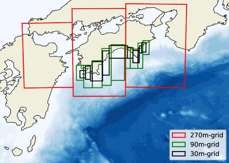
Figure 1: An example of three nested grid levels in the coast of Kochi Prefecture.

II-B Implementation

The RTi model was initially developed for the NEC SX-ACE system [4, 2], and later ported to the NEC SX-Aurora TSUBASA system [3] equipped with NEC Vector Engine (VE) processors [6, 7, 8]. The original code is implemented in Fortran 90 and parallelized using MPI only. NEC’s Fortran compiler is used to vectorize the code with the help of some vendor compiler directives to facilitate vectorization. Since neither intrinsics nor inline assembly is used, the code is functionally portable, but not necessarily performance-portable.

The domain decomposition is static and supplied via a configuration file by the user. One or more MPI ranks are assigned to each grid level. Each block in a grid level can be further decomposed into multiple ranks. In this case, one-dimensional domain decomposition is used. Although two-dimensional decomposition is preferable in terms of communication volume, it shortens the vectorized innermost loop. Since the vector register of a VE is 16384-wide and thus requires a long loop length for efficiency, one-dimensional decomposition is chosen over two-dimensional decomposition. Each rank is always assigned consecutive blocks. Further implementation details of the original code are described by its developers in their previous studies [3, 2].

III Related work

Tsunami-HySEA [12, 13, 14] is a state-of-the-art tsunami simulation code being developed at the University of Málaga that aims at realizing Faster Than Real Time (FTRT) tsunami simulation by utilizing GPUs. Tsunami-HySEA is developed in CUDA and uses MPI for multi-GPU parallelization. Similar to the code in this paper, Tsunami-HySEA also employs a nested grid system [12, 13] to reduce the computational load. The authors reported that an 8h-simulation of a tsunami hitting the Gulf of Cádiz with 5.5 million cells took 2.5 minutes to complete [15]. The code is highly tuned for NVIDIA GPUs, and takes advantage of features such as GPUDirect RDMA for inter-GPU communication, asynchronous CPU-GPU memory transfer and asynchronous file I/O.

TRITON-G [16] is another GPU-accelerated tsunami simulation code. The code is also developed in CUDA, and solves the non-linear spherical shallow water equations. Unlike the common nested grid system approach, this code adopts a quadtree-based approach for mesh refinement and Hilbert space-filling curve for load balancing. TRITON-G completed a 10-simulation covering a large portion of the Indian Ocean with approximately 33 million cells in under 10 using three NVIDIA Tesla P100 GPUs. This code was deployed as an operational model at the Regional Integrated Multi-Hazard Early Warning System for Africa and Asia (RIMES). In addition to Tsunami-HySEA and TRITON-G, a number of GPU-accelerated tsunami simulation codes have been developed in previous studies, most of which are implemented either in CUDA [17, 18] or CUDA Fortran [19].

JAGURS [20, 21] is a tsunami code originally based on the URSGA [22] hydrodynamic modeling tool. JAGURS significantly enhanced the scalability of URSGA by introducing a nested grid system and parallelizing the code using MPI and OpenMP. The performance of JAGURS was tested on the K computer, Japan’s former flagship supercomputer [21]. JAGURS was able to complete a 20s-simulation of a large-scale, high-resolution model consisting of 100 billion cells in 82s using the entire $82844$ nodes of the K computer. The model covered an area of 1000km $\times$ 780km and contained all of southwestern Japan. In addition, the authors also executed a 5h-simulation of a tsunami in the Nankai region of Japan with 680 million cells in 6625s using $8748$ nodes.

EasyWave [23, 24] is a simple tsunami simulation code that solves the linear long-wave theory equations in spherical coordinates. Since the nonlinear bottom friction is ignored, it is mainly intended for modeling far-field tsunamis. The code was originally developed as a sequential code and later ported to OpenMP, CUDA, OpenACC [23] and SYCL [24]. EasyWave does not employ MPI parallelism and thus does not scale out to multiple nodes, making it unsuitable for real-time tsunami simulation.

Although various tsunami simulation codes have been developed in the past, they are either optimized for a specific hardware platform  [15, 16, 17, 18, 19] or small-scale and simplified for performance analysis [24, 25]. To the best of our knowledge, this paper is the first work to present the migration process of a production-scale real-time tsunami simulation code to multiple hardware platforms.

IV Modernizing an operational tsunami simulator to support diverse hardware platforms

In this section, we first analyze the original code and then present our migration approach to support modern CPUs and GPUs. We further enhance the scalability of the migrated code by optimizing communication performance and improving load balance.

IV-A Analysis of the original RTi model

Figure 2 summarizes the subroutines called in the time integration loop. The time integration loop starts by solving Equation (1), which calculates the water level $\eta$ with the discharge fluxes $M$ and $N$. The obtained $\eta$ is sent from the child grid to the parent grid, and the boundary cells are exchanged between neighboring ranks in the same grid level. Then, Equations (2) and (3) are solved, which calculate the discharge fluxes, $M$ and $N$. Subsequently, the discharge fluxes are sent from the parent to the child grid, and the boundary cells are exchanged between neighbors. An iteration finishes by updating output data such as maximum water velocities, water levels and inundation depths, and swapping the double buffers. Out of the routines in Fig. 2, NLMASS (Equation 1) and NLMNT2 (Equations 2, 3) account for 60–70% of the runtime on an SX-Aurora TSUBASA system. Outside the time integration loop, there exist a number of routines including file I/O, initialization of data structures, fault model estimation and damage estimation. However, the total runtime of these routines is negligible compared to that of the time integration loop, and thus they are not the scope of this paper.

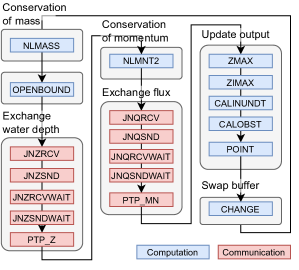
Figure 2: Overview of subroutines in the time integration loop.

Because of the employed finite-difference scheme, major computational kernels are two-dimensional stencil loops where each cell in a block can be updated independently. One key feature of this code is that a grid level is composed of many blocks of different sizes, and thus a loop that iterates over the blocks in a grid level exists.

Listing 1 shows the high-level structure of major loops, including the loop nests in the NLMASS and NLMNT2 routines. The outermost KK loop iterates over the blocks in a grid level. The inner I and J loops scan every cell in a single block. Although the code is designed in a configurable way such that the I and J loops can be either mapped to the y- or x-directions, in this paper we assume that the I and J loops iterate over the y- and x-directions of a block, respectively. There are no dependencies between the KK, J and I loops, and they can thus be executed in any order. There may be multiple J-I loop nests with different trip counts in a single KK loop.

Listing 1: Basic structure of major loops.

⬇

DO KK = BLK_PROC_ST, BLK_PROC_ED

! ...

DO J = JST_MN_X2(KK), JED_MN_X2(KK)

DO I = IST1_OWN(KK), IED2_OWN(KK)

! Update cell

END DO

END DO

! ...

END DO

It should be noted that the trip counts of the I and J loops depend on the loop index of the outer KK loop. This irregular loop structure cannot be simply collapsed using the collapse clause available in OpenACC and OpenMP, because the trip count of every nested loop to be collapsed needs to be predetermined and invariant. Furthermore, the trip count of the KK loops is short. For example, our dataset contains 60 blocks in total, which are distributed over multiple ranks. Thus, the KK loop alone does not provide enough parallelism for both GPUs and CPUs. The trip counts of both the J and I loops are in the order of $10000$.

Listing 2: Basic structure of major loops after migration.

⬇

!$omp parallel

DO KK = BLK_PROC_ST, BLK_PROC_ED

! ...

!$acc kernels async(MOD(KK,NSTREAMS))

!$acc loop collapse(2)

!$omp do

DO J = JST_MN_X2(KK), JED_MN_X2(KK)

!$omp simd

DO I = IST1_OWN(KK), IED2_OWN(KK)

! Update cell

END DO

!$omp end simd

END DO

!$omp end do nowait

!$acc end kernels

! ...

END DO

!$omp end parallel

!$acc wait

IV-B Migration of bottleneck routines

As described earlier, the code is already integrated into multiple tsunami early warning systems for providing tsunami inundation forecasts. Thus, rewriting a large portion of the codebase or porting the entire codebase to a different programming language or programming model is infeasible. We therefore aim to take a strategy that minimizes the code modifications.

The programming models we have considered are CUDA Fortran, OpenACC, OpenMP Target Offloading and Fortran Do Concurrent (DC). CUDA Fortran is a kernel-based programming model and requires considerable restructuring of the code; hence it is unsuitable for this migration. Fortran DC is promising [26, 27] since it is part of the Fortran 2008 language standard and thus can be used across CPUs and GPUs. However, it still requires modification of loops and even mixing OpenACC to obtain maximal performance [27]. Comparing the remaining two, recent studies agree that OpenACC generally outperforms OpenMP Target Offloading on NVIDIA GPUs due to compiler maturity [28, 29]. Thus, we decide to use OpenACC for GPUs. Although in principle OpenACC supports CPUs as well, a previous study [28] shows that it underperforms OpenMP by a large margin. Therefore, we use a combination of OpenACC for GPUs and OpenMP for CPUs in this paper.

Listing 2 shows the basic structure of loops after migrating to GPUs and CPUs. As the listing shows, there are no modifications except for the OpenACC and OpenMP directives, meeting the goal of retaining the original code structure.

On the GPU, the J and I loops are collapsed using the collapse clause and offloaded to the GPU. Even when the I and J loops are collapsed, they result in a total of less than $10^{6}$ iterations in most cases and cannot saturate the whole GPU. Furthermore, since a single kernel invocation finishes in approximately 50500 and kernel launches are synchronous by default in OpenACC, the kernel launch overhead becomes a non-negligible bottleneck. To hide the launch overhead, we take advantage of the async clause [30] in OpenACC. The async clause allows the host-side thread to continue execution, effectively hiding the kernel launch latency. In addition, the kernels are submitted to multiple asynchronous queues in a round-robin manner to increase the utilization of the GPU. Asynchronous queues are an abstraction of CUDA streams, and kernels submitted to different queues are asynchronously executed from one another. This takes advantage of the fact that different blocks can be independently updated.

The NLMNT2 routine requires additional work because it involves subroutine calls. The time derivative of discharge fluxes in the x- and y-directions for each cell are computed in routines XMMT and YMMT, which are invoked from the innermost loop body in NLMNT2. First, to compile these routines for the GPU, they are marked with acc routine directives as device functions. Second, scalar arguments are specified with the VALUE attribute to be passed by value. This is necessary because in Fortran, all arguments are passed by reference by default, and the compiler has to assume loop-carried dependence. Finally, we find that enabling Link Time Optimization (LTO) has a positive performance impact.

On the CPU, the J loop is mapped to threads and the I loop is mapped to vector lanes. To reduce the overhead of a parallel region, we enclose the entire loop nest with a parallel region. Furthermore, a nowait clause is added to the omp do directive to mitigate the overhead of implicit synchronization. Since the compiler fails to auto-vectorize the inner I loop in many cases, the I loop is explicitly vectorized by adding an omp simd directive. Similar to the GPU case, subroutine calls within the loop body become problematic since they prevent the compiler from vectorizing the loop. Thus, an attributes forceinline directive is added to the XMMT and YMMT routines to force them to be inlined in the loop body.

IV-C Communication optimization

On the GPU, only offloading the routines for computation in the time integration loop incurs expensive host-device memory copy for MPI communication. Thus, we utilize CUDA-aware MPI and GPUDirect RDMA (GDR) [31] to directly copy data between device memories and bypass the host. To enable the use of CUDA-aware MPI and GDR, we (1) place the MPI communication buffers on device memory, and (2) offload message packing and unpacking to the GPU.

IV-C1 Intra-grid exchange

Listing 3 shows a loop in the PTP_MN routine, which exchanges the discharge fluxes at the boundary cells between neighboring ranks in the same grid level. This specific loop nest packs the boundaries of two arrays VAL1 and VAL2 into a single communication buffer, BUF_SND1. Clearly, the loop-carried dependence on the buffer offset (ICNT) inhibits parallelization.

Listing 3: A loop in PTP_MN before optimization.

⬇

DO J = SFTN(6), SFTN(7)

DO I = SFTN(2), SFTN(3)

ICNT = ICNT + 1

BUF_SND1(ICNT) = VAL1(I,J,1)

BUF_SND1(ICNT+JNUM) = VAL1(I,J,2)

BUF_SND1(ICNT+2*JNUM) = VAL2(I,J)

END DO

END DO

Listing 4 shows the same loop after optimization. Since the trip counts of both I and J loops can be pre-determined, we calculate the buffer offset from the loop indices of the two loops. The two loops are collapsed using a collapse clause and offloaded to the GPU as a single kernel. A similar optimization is applied to the PTP_Z routine as well.

Listing 4: A loop in PTP_MN after optimization.

⬇

!$acc kernels

!$acc loop collapse(2) independent

DO J = SFTN(6), SFTN(7)

DO I = SFTN(2), SFTN(3)

ICNT = (I- SFTN(2) + 1) + (J - SFTN(6)) * (SFTN(3) - SFTN(2) + 1)

BUF_SND1(ICNT) = VAL1(I,J,1)

BUF_SND1(ICNT+JNUM) = VAL1(I,J,2)

BUF_SND1(ICNT+2*JNUM) = VAL2(I,J)

END DO

END DO

!$acc end kernels

IV-C2 Inter-grid exchange

Listing 5 shows an excerpt from the JNZSND routine. This routine sends the water levels at the boundary cells of a child grid to its parent grid. Because each rank may have multiple blocks and a child block can have multiple parent blocks, each rank may need to send multiple boundary regions to multiple receiver ranks. In this routine, the outer NN1 loop iterates over the receiver ranks, and the inner NN2 loop iterates over the boundaries of multiple blocks. The JNZ_SND and JNZ_SND_NO arrays hold information such as the receiver of the boundary and the two-dimensional range of the boundary. The JJ loop scans the cells of a boundary and reduces the resolution by averaging the water levels in a 3$\times$3 cell. The average water level is then written to BUFS, the MPI communication buffer. ICNT_WK keeps track of the current offset in the communication buffer.

Listing 5: A loop in JNZSND before optimization.

⬇

DO NN1 = 1, NUM_JNZ_SND_SZ ! iterate over receivers

ICNT_WK = 0

DO NN2 = 1, JNZ_SND_SZ(3,NN1) ! iterate over boundaries

NPCNT = JNZ_SND_NO(NN2,NN1)

IF(JNZ_SND(2,NPCNT)==1.OR.JNZ_SND(2,NPCNT)==2)THEN

JSL = JNZ_SND(7,NPCNT)

JEL = JNZ_SND(8,NPCNT)

JJS = JNZ_SND(4,NPCNT) - 3

IIS = JNZ_SND(3,NPCNT)

...

DO JJ=JSL,JEL

JJS = JJS + 3

SUMZ = 0.0

DO J=JJS,JJS+2 ! calculate average

DO I=IIS,IIS+2

SUMZ = SUMZ + ZZ(I,J,2)

END DO

END DO

ZZZ = SUMZ * (1.0/9.0)

ICNT_WK = ICNT_WK + 1

BUFS(ICNT_WK,NN1) = ZZZ

END DO

ELSE IF

...

END IF

END DO

END DO

Evidently, the incremental update of the offset ICNT_WK introduces a loop-carried dependence and prevents parallelization. In contrast to the intra-grid neighbor exchange routines, ICNT_WK cannot be computed from just the loop indices because the sizes of the boundaries are irregular. Instead, we pre-compute a table that contains the size of each boundary region and its offset in the communication buffer, taking advantage of the fact that the grid organization and domain decomposition are fixed during runtime. Listing 6 shows the JNZSND routine after optimization. JNZ_BUFS_OFS holds the pre-computed offsets. The offset of the NN2-th boundary sent to rank NN1 is obtained by JNZ_BUFS_OFS(NN2,NN1). Using this pre-computed offset table, all boundary cells can be copied to the communication buffer in parallel. We also insert acc loop gang and vector directives so that a thread block is assigned to each boundary and a thread is assigned to each cell within the boundary.

The JNZ_RCVWAIT routine for unpacking the water depth at the receiver rank is also optimized using a pre-computed offset table. The JNQ_SND and JNQ_RCVWAIT routines for exchanging the discharge fluxes are also optimized in a similar manner.

Listing 6: A loop in JNZSND after optimization.

⬇

DO NN1 = 1, NUM_JNZ_SND_SZ

!$acc kernels default(present) async

!$acc loop gang independent

DO NN2 = 1, JNZ_SND_SZ(3,NN1)

NPCNT = JNZ_SND_NO(NN2,NN1)

IF(JNZ_SND(2,NPCNT)==1.OR.JNZ_SND(2,NPCNT)==2)THEN

...

!$acc loop vector independent

DO JJ=JSL,JEL

JJS = JJS + 3

SUMZ = 0.0

!$acc loop seq collapse(2)

DO J=JJS,JJS+2

DO I=IIS,IIS+2

SUMZ = SUMZ + ZZ(I,J,2)

END DO

END DO

ZZZ = SUMZ * (1.0/9.0)

BUFS(JNZ_BUFS_OFS(NN2,NN1)+JJ-JSL+1,NN1) = ZZZ

END DO

ELSE IF

! ...

END IF

END DO

!$acc end kernels

END DO

!$acc wait

IV-D Load-balancing improvement

The original domain decomposition algorithm equalizes the total number of cells assigned to each rank [2]. However, since our code launches a kernel for each block, a non-negligible cost is incurred for each block. This is apparent in Fig. 3, which shows the runtime breakdown when executing the simulation on 16 ranks on an NVIDIA A100 system. The breakdown clearly shows a severe load imbalance, where on some of the ranks such as ranks 6 and 16, the NLMASS and NLMNT2 routines take a considerably longer time than on the other ranks.

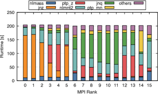
Figure 3: Breakdown of runtime before adjusting the work imbalance.

Figure 4 shows the number of cells and the number of blocks assigned to each rank. Although ranks 3 to 15 have roughly equal numbers of cells, ranks 6 and 15 have more than 16 blocks assigned. This clearly shows that assigning too many blocks to a single rank increases its runtime and potentially causes load imbalance. Note that ranks 0 to 2 are assigned to grid levels 1 to 3, respectively, and thus have fewer cells. This is because of the limitation of the original code that does not allow assigning multiple grid levels to a single rank.

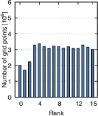
(a) Number of cells

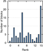
(b) Number of blocks

Figure 4: Domain decomposition before optimization.

To alleviate this load imbalance, we consider two methods in this paper. In the first method, we modify the code to launch a single kernel regardless of the number of blocks assigned to a rank. In the second method, we quantify the per-block cost and use it to optimize the domain decomposition. Each method is described in detail in the following sections.

IV-D1 Merging multiple kernels

The basic idea of this method is to collapse the outer two loops. The main reason that the outermost loop and the inner loops cannot be trivially collapsed is that the trip counts of the inner I and J loops depend on the KK loop. Listing 7 shows the basic loop structure after outer loops. Our idea is to calculate the maximum trip count of the J loop and “pad” the iteration space in the J-dimension. In this way, the trip count of the J loop becomes invariant, and thus the KK and J loops can be collapsed using a collapse clause. We then explicitly assign the collapsed KK-J loop and I loop to gangs and vectors, respectively (thread blocks and threads in NVIDIA terminology). In the case where the outer KK loop contains multiple J-I loops, loop fission is first applied to split the KK loop into multiple loops.

Listing 7: Basic structure of major loops after collapsing outer loops.

⬇

JSZ = MAXVAL(JED_MN_X2 - JST_MN_X2)

!$acc parallel

!$acc loop collapse(2) gang

!$omp parallel do

DO KK = BLK_PROC_ST, BLK_PROC_ED

DO J = JST_MN_X2(KK), JST_MN_X2(KK) + JSZ

IF (J > JED_MN_X2(KK)) CYCLE

!$acc loop vector

!$omp simd

DO I = IST1_OWN(KK), IED2_OWN(KK)

! Update cell

END DO

!$omp end simd

END DO

END DO

!$omp end parallel do

!$acc end parallel loop

IV-D2 Tuning the domain decomposition

In this method, we first construct an empirical performance model of the computationally intensive routine and use it to adjust the domain decomposition. We first implement a microbenchmark to measure the runtime of the most time-consuming NLMNT2 routine. The benchmark repeatedly calls the NLMNT2 routine for a given block and measures the runtime. Kernels are launched asynchronously on multiple streams as described in Section IV-B. Figure 5 plots the runtime of NLMNT2 for a given block with respect to its number of cells. The runtime clearly exhibits a linear trend and can be fitted by a linear function $y=1.09\cdot 10^{-4}x+46.2$ with a high $R^{2}$ score of 0.942.

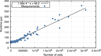
Figure 5: Runtime of NLMNT2 routine with respect to the number of cells of a block.

Since each rank has one or more blocks, we estimate the runtime of a rank as the total runtime of all blocks in a rank. We model the runtime of rank as follows:

$$T=\sum_{i=1}^{n}{1.09\cdot 10^{-4}b_{i}+46.2}\,[\unit{}],$$ (5)

where $n$ is the total number of blocks and $b_{i}$ is the number of cells in the $i$-th block. Figure 6 compares the actual and predicted runtime of the NLMNT2 routine using this performance model. Although the prediction accuracy is generally high, interestingly, the actual runtime is consistently shorter than the predicted runtime. This is likely due to a better overlap between different blocks.

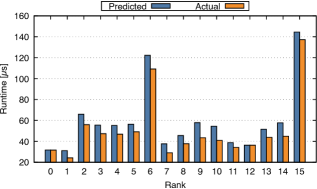
Figure 6: Runtime of NLMNT2 routine predicted with the performance model.

We now use this performance model to optimize the domain decomposition such that the estimated runtime of the NLMNT2 routine is equalized among ranks. Since each rank needs to be assigned consecutive blocks, we assume “separators” between ranks as illustrated in Fig. 7 and optimize the positions of the separators. Algorithm 1 shows the heuristic algorithm. The algorithm is based on the hill climbing method, and iteratively improves the positions of the separators, i.e., domain decomposition. In each iteration, one separator is randomly chosen and moved to a random position between the preceding and succeeding separators. The new position is accepted if the score function improves; otherwise, the separator is restored to its previous position. This procedure is repeatedly executed for a fixed number of iterations.

Figure 7: Overview of domain decomposition tuning.

Result: List of separator positions

1 Randomly initialize positions of all separators;

2 for number of iterations do

3       Randomly select a separator;

4       Move the separator to a random position between the preceding and succeeding separators;

5       Compute score using the performance model;

6       if score does not improve then

7             Restore the position of the separator;

8            

9      

Algorithm 1 Algorithm for optimization the domain decomposition.

Two score functions, which are the variance of the predicted runtime and maximum predicted runtime, are used. This is because if the maximum runtime is used, the score changes only if the separator adjacent to the rank with the highest predicted runtime is moved. Thus, the optimization stagnates if only the maximum runtime is used. Contrastingly, the variance of runtime always changes if the runtime of any rank changes. Minimizing the variance, however, does not necessarily result in minimizing the maximum runtime. Thus, we combine the two score functions to accelerate the optimization: in the first phase, the variance of the predicted runtime is used, and in the second phase, the maximum predicted runtime is used.

Figure 8 shows the runtime breakdown after optimizing the domain decomposition. Clearly, the load balance is significantly improved, and the synchronization wait time in the communication routines such as JNQ and PTP_Z is reduced. As a result, the maximum runtime of the NLMNT2 routine is reduced from 99 to 54, and the total runtime is reduced from 200 down to 126. Figure 9 shows the domain decomposition after optimization. It can be seen that the number of cells is no longer balanced across ranks, but the maximum number of blocks is significantly reduced. Since ranks 6 and 16 still have more blocks assigned compared to the other ranks, the number of cells is smaller in order to offset for the larger number of blocks.

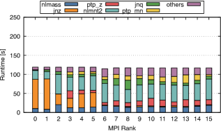
Figure 8: Breakdown of runtime after adjusting the load imbalance.

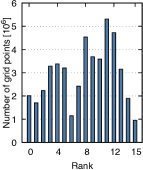
(a) Number of cells

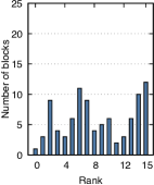
(b) Number of blocks

Figure 9: Domain decomposition after optimization.

V Performance evaluation

In this section, we evaluate the performance of the migrated tsunami simulation code. We first quantify the performance benefit of each optimization, and then compare the performance of our code on multiple HPC systems using VE, CPU, and GPU.

V-A Evaluation environments

In this evaluation, we use a model designed to provide tsunami inundation forecasts for Kochi Prefecture in Japan. Kochi Prefecture is located at the Pacific coast of Japan and close to the Nankai Trough, which is the source of Nankai megathrust earthquakes that have caused devastating damages through history. Table I shows the organization of the grids in the Kochi model. The model covers an area of 1025km$\times$1287km including the coastline of Kochi. The spatial resolution $\Delta x$ of the finest grid is 10m and the $\Delta x$ of the coarsest grid is $\qty{10}{m}\cdot 3^{4}=\qty{810}{m}$. The time resolution $\Delta t$ is 0.2s across all grid levels.

Table II summarizes the four HPC systems used in this evaluation: AOBA-S [32] at Tohoku University, SQUID [33] at Osaka University, and Pegasus [34] at University of Tsukuba. AOBA-S is an SX-Aurora TSUBASA system using the third-generation Vector Engine processors. SQUID consists of several node types. We used the CPU nodes equipped with IceLake-generation Intel CPUs and the GPU nodes equipped with NVIDIA A100 SXM4 GPUs. Pegasus is a supercomputer equipped with NVIDIA H100 PCIe GPUs.

TABLE I: Grid organization of the Kochi model.

Grid level	$\Delta x$	# of blocks	# of cells
1	810	1	$2012940$
2	270	3	$1703484$
3	90	9	$2230056$
4	30	11	$9863424$
5	10	60	$31401540$
Total		84	$47211444$

TABLE II: HPC systems used for evaluation.

	AOBA-S [32]	SQUID [33] (GPU node)	SQUID (CPU node)	Pegasus [34]
CPU	AMD EPYC 7763	Intel Xeon Platinum 8368 $\times$2	Intel Xeon Platinum 8368 $\times$2	Intel Xeon Platinum 8468 $\times$1
Memory	DDR4 256GB	DDR4 512GB	DDR4 256GB	DDR5 128GB
Accelerator	NEC Vector Engine Type 30A $\times$8	NVIDIA A100 (SXM4) $\times$8	N/A	NVIDIA H100 (PCIe) $\times$1
Interconnect	InfiniBand NDR200 $\times$2	InfiniBand HDR100 $\times$4	InfiniBand HDR200 $\times$1	InfiniBand NDR200 $\times$1
Compilers	NEC Fortran 5.2.0	NVIDIA HPC SDK 22.11	Intel oneAPI 2023.2.4	NVIDIA HPC SDK 24.1
				Intel oneAPI 2023.0.0

V-B Asynchronous and concurrent kernel launch

To quantify the performance benefit of the asynchronous and concurrent kernel launch method employed in our code, we vary the number of asynchronous queues and measure the performance of the NLMNT2 routine. Figure 10 shows the runtime of the NLMNT2 routine normalized by its runtime when launching the kernels synchronously. When the number of asynchronous queues is one, i.e., the kernels are launched asynchronously but not concurrently, the speedup over synchronous launch ranges from 1.3$\times$ to 2.0$\times$. The speedup is achieved by hiding the kernel launch latency and primarily depends on the number of blocks assigned to the rank because it is proportional to the number of kernel launches.

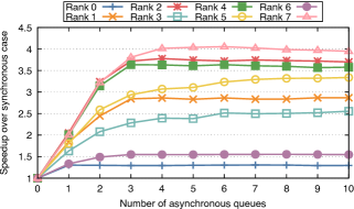
Figure 10: Runtime of NLMNT2 routine with respect to the number of asynchronous queues on NVIDIA A100.

The speedup improves with the number of asynchronous queues and saturates at four queues. The maximum speedup ranges from 1.3$\times$ to 4.0$\times$ depending on the rank. This indicates that the GPU is saturated when kernels are submitted concurrently to four queues.

To verify that the hardware utilization improves with the number of asynchronous queues, we measured the GPU and memory utilization using the NVIDIA Management Library (NVML). The definitions of these metrics are as follows:

GPU utilization

Fraction of time where one or more kernels were running on the GPU.

Memory utilization

Fraction of time where the device memory was accessed.

We also tried NVIDIA Nsight Compute but found out that profiling a range including many small and short kernel launches leads to inaccuracies.

Figure 11 shows the utilization rates with respect to the number of queues. Figure 11(a) shows that the GPU is left idle when kernels are synchronously launched. The idle time is significantly reduced when kernels are asynchronously launched. Note that the GPU utilization only reflects whether a kernel is being executed on the GPU, and does not reflect the resource utilization of individual kernels. Figure 11(b) shows that the memory utilization gradually increases with the number of asynchronous queues, and saturates at four queues. This aligns with the saturation of speedup observed in Fig. 10. Based on these results, we set the number of asynchronous queues to four in the following evaluation experiments.

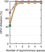
(a) GPU

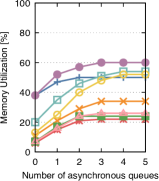
(b) Memory

Figure 11: GPU and memory utilization measured using NVML (legend is identical to that of Fig. 10).

V-C Load-balancing methods

We evaluate the effectiveness of the two methods for improving load balance by comparing the runtime of the NLMNT2 routine before and after improving the load balance. Figure 12 shows the runtime of the NLMNT2 routine on each rank. As the figure shows, both methods are able to improve the load imbalance significantly. The maximum runtime of the NLMNT2 routine in the baseline code is 139. This is reduced down to 56 when collapsing the outer loops, and to 73 when using the optimized domain decomposition. At first sight, the first option seems to be a better choice. However, collapsing the outer loops actually degrades performance on CPUs as shown in Fig. 13. This is because on a GPU, the performance gain thanks to collapsing the outer loops outweighs the extra cost incurred by padding the iteration space, but on a CPU, the load balance is already good in the baseline case and thus collapsing the outer loop only causes a negative impact on the performance.

Of course, one could use the loop collapsed version on GPUs and the baseline version on CPUs and VEs. However, this conflicts with the goal of having a single codebase for all platforms. Therefore, we use the second domain decomposition method in the following evaluation.

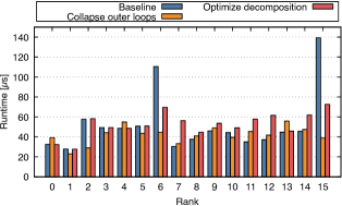
Figure 12: Runtime of NLMNT2 routine before and after improving the load balance on NVIDIA A100.

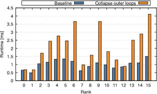
Figure 13: Runtime of NLMNT2 routine before and after improving the load balance on Intel Xeon Platinum 8468.

V-D Communication optimization

To assess the impact of the intra- and inter-grid communication routine optimization, we compare a naive implementation and the GPU-offloaded implementation of the communication routines. Figure 16 shows the runtime of a six-hour tsunami simulation using the Kochi model on SQUID (GPU). The naive implementation copies the boundary cells between the GPU and CPU before and after communication. Offloading the message packing and unpacking to the GPU and utilizing GDR greatly improves the runtime by a factor of 2.96$\times$ and 1.09$\times$ on 8 and 16 ranks, respectively. This is because the latency of host-device memory copies is eliminated and the frequency of host-device synchronization is reduced. On 32 ranks, however, the runtime increases by 1.41$\times$ due to low inter-GPU communication performance.

After tweaking various parameters in UCX [35], a low-level communication library used by Open MPI, we found that the default message size threshold for switching from eager to rendezvous protocol was suboptimal. This issue was resolved by enabling a UCX parameter UCX_PROTO_ENABLE, which activates a new mechanism for automatically selecting the optimal protocol. In addition, we restricted the InfiniBand NIC used by each GPU using the UCX_NET_DEVICES parameter to reduce the GPU-NIC communication latency. Since a SQUID GPU node has four NICs and eight GPUs distributed over four PCIe switches, we configured UCX such that each GPU uses the NIC connected to the same PCIe switch as the GPU. As a result of tuning UCX, the total runtime improved by 1.27$\times$ on 16 ranks and 1.62$\times$ on 32 ranks.

Figure 16 shows the simulation runtime on Pegasus (GPU). On Pegasus, utilizing GDR results in a speedup ranging from 2.95–3.23$\times$, larger than that on SQUID. This is because the bottleneck routines (NLMNT2 and NLMASS) run faster on the H100 GPU than on the A100 GPU, and thus communication tends to become a bottleneck as the number of GPUs scales out. On Pegasus, UCX tuning is not required because UCX_PROTO_ENABLE is enabled by default due to a newer UCX version. In addition, GPU-NIC affinity is also not needed because each compute node is equipped with one GPU and one NIC.

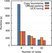
.5 .5

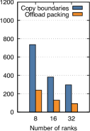
Figure 14: SQUID (GPU)

Figure 15: Pegasus (GPU)

Figure 16: Impact of communication routine optimization on the simulation runtime.

V-E Comparison across hardware platforms

Figure 17 compares the runtime for completing a six-hour tsunami simulation using the Kochi model on SQUID, AOBA-S and Pegasus. To make a fair comparison, we fix the number of CPUs or GPUs and compare the runtime. The MPI process count is tuned for each system, that is, one process per socket on SQUID (CPU) and four processes per socket on Pegasus (CPU). On SQUID (GPU) and Pegasus (GPU), one process is launched per GPU.

When using four sockets, AOBA-S marks 640, which marginally fails to achieve the 10 deadline. SQUID (CPU) and Pegasus (CPU) achieve 1636 and 1476, respectively, both being twice as slow as AOBA-S. This is due to the excellent memory bandwidth of the VE processor used in AOBA-S. The GPU version cannot be run because efficiently sharing a single GPU by multiple processes requires Multi-Instance GPU (MIG) or Multi-Process Service (MPS), both of which are unavailable on Pegasus and SQUID.

When using eight sockets, all of AOBA-S, SQUID (GPU) and Pegasus (GPU) complete within 600, successfully meeting the 10-10-10 challenge. Pegasus (GPU) is the fastest, followed by AOBA-S and then SQUID (GPU). This order is consistent with the order of effective memory bandwidth of the processors used in these systems. With 16 sockets, SQUID (CPU) and Pegasus (CPU) exhibit a super-linear speedup, and the performance difference between the CPU-based systems and the rest becomes smaller. This is due to the large L3 cache size where the working set can fit on L3 cache as the number of sockets increases. In fact, the L3 cache miss rate measured using the LIKWID [36] profiling tool on 8, 16 and 32 ranks is 33%, 14%, 3%, respectively. With 32 sockets, the runtime is less than 3 on all systems, and just 82 on Pegasus (GPU). At this scale, the cache hit rate is high on all systems, making the code cache bandwidth-bound.

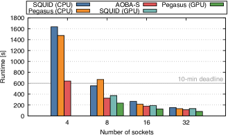
Figure 17: Runtime of a six-hour tsunami simulation using the Kochi model on different HPC systems.

VI Conclusions & Future Work

In this paper, we migrated the RTi model, a production-scale tsunami propagation and inundation simulation code specifically designed for vector processors, to the latest CPUs and GPUs. The migration is conducted in a minimally invasive manner, i.e., retaining the original loop structures and minimizing the amount of code modifications, to reduce the testing and maintenance costs. A combination of directive-based programming models and target-specific optimizations including load balance improvement for GPUs are applied to achieve this goal successfully. We demonstrated that the migrated code runs efficiently on recent CPUs, GPUs and vector processors. A six-hour tsunami simulation using over 47 million cells completes in less than 2.5 minutes on 32 Intel Sapphire Rapids CPUs and 1.5 minutes on 32 NVIDIA H100 GPUs. These results demonstrate that the code enables broader access to accurate tsunami inundation forecasts in the future.

The load balancing method presented in this paper could be applied to other large-scale codes, especially multi-block structured simulation codes that follow a similar parallelization strategy. The key idea of our method is to model the kernel runtime including the GPU offloading overhead, and use the performance model to optimize the domain decomposition with a local search. We hope to extend this methodology to different domain decomposition schemes and computational kernels.

References

- [1] E. Bernard and V. Titov, “Evolution of tsunami warning systems and products,” Philosophical Transactions of the Royal Society A: Mathematical, Physical and Engineering Sciences, vol. 373, no. 2053, 2015.
- [2] T. Inoue, T. Abe, S. Koshimura, A. Musa, Y. Murashima, and H. Kobayashi, “Development and validation of a tsunami numerical model with the polygonally nested grid system and its MPI-parallelization for real-time tsunami inundation forecast on a regional scale,” Journal of Disaster Research, vol. 14, no. 3, pp. 416–434, 2019.
- [3] A. Musa, T. Abe, T. Kishitani, T. Inoue, M. Sato, K. Komatsu, Y. Murashima, S. Koshimura, and H. Kobayashi, “Performance Evaluation of Tsunami Inundation Simulation on SX-Aurora TSUBASA,” in 19th International Conference on Computational Science, vol. 11537 LNCS, 2019, pp. 363–376.
- [4] A. Musa, O. Watanabe, H. Matsuoka, H. Hokari, T. Inoue, Y. Murashima, Y. Ohta, R. Hino, S. Koshimura, and H. Kobayashi, “Real-time tsunami inundation forecast system for tsunami disaster prevention and mitigation,” Journal of Supercomputing, vol. 74, no. 7, pp. 3093–3113, 2018.
- [5] R. Egawa, K. Komatsu, S. Momose, Y. Isobe, A. Musa, H. Takizawa, and H. Kobayashi, “Potential of a modern vector supercomputer for practical applications: performance evaluation of SX-ACE,” Journal of Supercomputing, vol. 73, no. 9, pp. 3948–3976, 2017.
- [6] K. Komatsu, S. Momose, Y. Isobe, O. Watanabe, A. Musa, M. Yokokawa, T. Aoyama, M. Sato, and H. Kobayashi, “Performance evaluation of a vector supercomputer SX-aurora TSUBASA,” in Proceedings - International Conference for High Performance Computing, Networking, Storage, and Analysis, SC 2018. IEEE, 2018, pp. 685–696.
- [7] R. Egawa, S. Fujimoto, T. Yamashita, D. Sasaki, Y. Isobe, Y. Shimomura, and H. Takizawa, “Exploiting the Potentials of the Second Generation SX-Aurora TSUBASA,” in Proceedings of PMBS 2020: Performance Modeling, Benchmarking and Simulation of High Performance Computer Systems, vol. 2, 2020, pp. 39–49.
- [8] K. Takahashi, S. Fujimoto, S. Nagase, Y. Isobe, Y. Shimomura, R. Egawa, and H. Takizawa, “Performance Evaluation of a Next-Generation SX-Aurora TSUBASA Vector Supercomputer,” in 38th International Conference on High Performance Computing (ISC High Performance 2023), 2023, pp. 359–378.
- [9] H. Jun, J. Cho, K. Lee, H. Y. Son, K. Kim, H. Jin, and K. Kim, “HBM (High bandwidth memory) DRAM technology and architecture,” 2017 IEEE 9th International Memory Workshop, IMW 2017, pp. 1–4, 2017.
- [10] C. Goto, Y. Ogawa, N. Shuto, and F. Imamura, “Numerical method of tsunami simulation with the leap-frog scheme,” IUGG/IOC TIME Project Intergovernmental Oceanographic Commission of UNESCO, Manuals and Guides, vol. 35, pp. 1–126, 1997.
- [11] F. Imamura, A. C. Yalçiner, and G. Ozyurt, “Tsunami modelling manual,” Tsunami Modelling Manual, no. April, p. 58, 2006.
- [12] J. Macías, A. Mercado, J. M. González-Vida, S. Ortega, and M. J. Castro, “Comparison and Computational Performance of Tsunami-HySEA and MOST Models for LANTEX 2013 Scenario: Impact Assessment on Puerto Rico Coasts,” Pure and Applied Geophysics, vol. 173, no. 12, pp. 3973–3997, 2016.
- [13] J. Macías, M. J. Castro, S. Ortega, C. Escalante, and J. M. González-Vida, “Performance Benchmarking of Tsunami-HySEA Model for NTHMP’s Inundation Mapping Activities,” Pure and Applied Geophysics, vol. 174, no. 8, pp. 3147–3183, 2017.
- [14] J. Macías, M. J. Castro, S. Ortega, and J. M. González-Vida, “Performance assessment of Tsunami-HySEA model for NTHMP tsunami currents benchmarking. Field cases,” Ocean Modelling, vol. 152, no. August 2019, p. 101645, 2020.
- [15] B. Gaite, J. Macías, J. V. Cantavella, C. Sánchez-Linares, C. González, and L. C. Puertas, “Analysis of Faster-Than-Real-Time (FTRT) Tsunami Simulations for the Spanish Tsunami Warning System for the Atlantic,” GeoHazards, vol. 3, no. 3, pp. 371–394, 2022.
- [16] M. A. Acuña and T. Aoki, “Tree-based mesh-refinement GPU-accelerated tsunami simulator for real-time operation,” Natural Hazards and Earth System Sciences, vol. 18, no. 9, pp. 2561–2602, 2018.
- [17] S. Koshimura, K. Katsuki, and Y. Shigeto, “Reatl-time tsunami simulation using GPU,” Journal of Japan Society of Civil Engineers, Ser. B2 (Coastal Engineering), vol. 66, no. 1, pp. 191–195, 2010.
- [18] M. T. Satria, B. Huang, T. J. Hsieh, Y. L. Chang, and W. Y. Liang, “GPU acceleration of tsunami propagation model,” IEEE Journal of Selected Topics in Applied Earth Observations and Remote Sensing, vol. 5, no. 3, pp. 1014–1023, 2012.
- [19] Y. Yuan, F. Shi, J. T. Kirby, and F. Yu, “FUNWAVE-GPU: Multiple-GPU Acceleration of a Boussinesq-Type Wave Model,” Journal of Advances in Modeling Earth Systems, vol. 12, no. 5, 2020.
- [20] T. Baba, N. Takahashi, Y. Kaneda, Y. Inazawa, and M. Kikkojin, “Tsunami inundation modeling of the 2011 Tohoku earthquake using three-dimensional building data for Sendai, Miyagi prefecture, Japan,” Advances in Natural and Technological Hazards Research, vol. 35, pp. 89–98, 2014.
- [21] T. Baba, K. Ando, D. Matsuoka, M. Hyodo, T. Hori, N. Takahashi, R. Obayashi, Y. Imato, D. Kitamura, H. Uehara, T. Kato, and R. Saka, “Large-scale, high-speed tsunami prediction for the Great Nankai Trough Earthquake on the K computer,” International Journal of High Performance Computing Applications, vol. 30, no. 1, pp. 71–84, 2016.
- [22] J. D. Jakeman, O. M. Nielsen, K. V. Putten, R. Mleczko, D. Burbidge, and N. Horspool, “Towards spatially distributed quantitative assessment of tsunami inundation models,” Ocean Dynamics, vol. 60, no. 5, pp. 1115–1138, 2010.
- [23] S. Christgau, J. Spazier, B. Schnor, M. Hammitzsch, A. Babeyko, and J. Wachter, “A comparison of CUDA and OpenACC: Accelerating the Tsunami Simulation EasyWave,” in 27th International Conference on Architecture of Computing Systems Workshops (ARCS 2014), 2014.
- [24] S. Christgau and T. Steinke, “Porting a Legacy CUDA Stencil Code to oneAPI,” in 34th International Parallel and Distributed Processing Symposium Workshops (IPDPSW 2020), 2020, pp. 359–367.
- [25] M. Büttner, C. Alt, T. Kenter, and H. Köstler, “Enabling Performance Portability for Shallow Water Equations on CPUs , GPUs , and FPGAs with SYCL,” in Platform for Advanced Scientific Computing Conference (PASC ’24). Association for Computing Machinery, 2024.
- [26] M. Alkan, B. Q. Pham, J. R. Hammond, and M. S. Gordon, “Enabling Fortran Standard Parallelism in GAMESS for Accelerated Quantum Chemistry Calculations,” Journal of Chemical Theory and Computation, vol. 19, no. 13, pp. 3798–3805, 2023.
- [27] R. M. Caplan, M. M. Stulajter, and J. A. Linker, “Acceleration of a production Solar MHD code with Fortran standard parallelism: From OpenACC to ’do concurrent’,” International Parallel and Distributed Processing Symposium Workshops (IPDPSW 2023), pp. 582–590, 2023.
- [28] T. Deakin, A. Poenaru, T. Lin, and S. McIntosh-Smith, “Tracking Performance Portability on the Yellow Brick Road to Exascale,” in P3HPC 2020: International Workshop on Performance, Portability and Productivity in HPC, 2020.
- [29] H. Brunst, S. Chandrasekaran, F. Ciorba, N. Hagerty, R. Henschel, G. Juckeland, and J. Li, “First Experiences in Performance Benchmarking with the New SPEChpc 2021 Suites,” in 22nd international Symposium on Cluster, Cloud and Internet Computing (CCGrid 2022), 2022.
- [30] S. Chandrasekaran and G. Juckeland, OpenACC for Programmers: Concepts and Strategies, 1st ed. Addison-Wesley Professional, 2017.
- [31] S. Potluri, K. Hamidouche, A. Venkatesh, D. Bureddy, and D. K. Panda, “Efficient inter-Node MPI communication using GPUDirect RDMA for InfiniBand clusters with NVIDIA GPUs,” International Conference on Parallel Processing, pp. 80–89, 2013.
- [32] H. Takizawa, K. Takahashi, Y. Shimomura, R. Egawa, K. Oizumi, S. Ono, T. Yamashita, and A. Saito, “AOBA: The Most Powerful Vector Supercomputer in the World,” in Sustained Simulation Performance 2022, 2024, pp. 71–81.
- [33] S. Date, Y. Kido, Y. Katsuura, Y. Teramae, and S. Kigoshi, “Supercomputer for Quest to Unsolved Interdisciplinary Datascience (SQUID) and its Five Challenges,” in Sustained Simulation Performance 2021, 2023, pp. 1–19.
- [34] Center for Computational Sciences, “Pegasus – Big memory supercomputer.” [Online]. Available: https://www.ccs.tsukuba.ac.jp/eng/supercomputers/#Pegasus
- [35] P. Shamis, M. G. Venkata, M. G. Lopez, M. B. Baker, O. Hernandez, Y. Itigin, M. Dubman, G. Shainer, R. L. Graham, L. Liss, Y. Shahar, S. Potluri, D. Rossetti, D. Becker, D. Poole, C. Lamb, S. Kumar, C. Stunkel, G. Bosilca, and A. Bouteiller, “UCX: An Open Source Framework for HPC Network APIs and Beyond,” in 23rd Annual Symposium on High-Performance Interconnects (HOTI 2015). IEEE, 2015, pp. 40–43.
- [36] J. Treibig, G. Hager, and G. Wellein, “LIKWID: A Lightweight Performance-Oriented Tool Suite for x86 Multicore Environments,” in 39th International Conference on Parallel Processing Workshops, sep 2010, pp. 207–216.