Dynamics of gauged Q-balls in three spatial dimensions
Abstract
We investigate the dynamics of gauged Q-balls using fully three-dimensional numerical simulations. We consider two different scenarios: first, the classical stability of gauged Q-balls with respect to generic three-dimensional perturbations, and second, the behaviour of gauged Q-balls during head-on and off-axis collisions at relativistic velocities. With regards to stability, we find that there exist gauged Q-ball configurations which are classically stable in both logarithmic and polynomial scalar field models. With regards to relativistic collisions, we find that the dynamics can depend on many different parameters such as the collision velocity, relative phase, relative charge, and impact parameter of the colliding Q-balls.
I Introduction
Q-balls are non-topological solitons that arise in scalar field theories admitting a symmetry and a non-linear attractive potential. First described by Coleman [1, *Coleman1986], they have garnered significant attention in recent years due to their potential relevance to early-Universe cosmology (where they may act as dark matter candidates [3, 4]) and in condensed matter experiments (where they serve as relativistic analogues to various condensed matter solitons [5, 6]). Q-balls also hold considerable theoretical interest as smooth, classical field configurations which constitute a rudimentary model of a particle.
An extension to the basic Q-ball theory can be made through the introduction of a gauge field. This gives rise to so-called gauged Q-balls which couple to the electromagnetic field and carry an electric charge [7]. While gauged Q-balls share some similarities with ordinary (non-gauged) Q-balls, the additional electromagnetic coupling can also lead to several distinct features. For example, it may place restrictions on their allowable size and charge [8, 9], change their dynamical behaviour [10, 11], and even give rise to new types of solutions in the model (such as shell-shaped structures [12, 8, 13]). It has also been speculated that the repulsive Coulomb force arising from a gauged Q-ball might serve as a destabilizing mechanism which eventually destroys it [14]. This is an important issue because one should expect gauged Q-balls to be robust against generic perturbations in order to be considered viable physical objects. However, the stability analysis of these objects is challenging because the application of standard methods for establishing classical stability (such as linear perturbation analyses or known stability theorems) are hindered by the presence of the gauge field. In particular, it is known that gauged Q-balls can be classically stable against spherically-symmetric and axially-symmetric perturbations [14, 10], but the case of general three-dimensional perturbations has yet to be explored.
In the present work, we address this problem of gauged Q-ball stability by performing fully non-linear numerical evolutions of the equations of motion in three spatial dimensions. For gauged Q-balls in both logarithmic and polynomial scalar field models, we find numerical evidence for solutions which are classically stable against generic three-dimensional perturbations over long dynamical timescales. In these cases, we find that the stable gauged Q-balls respond to the perturbations by oscillating continuously or weakly radiating before evolving toward a state that is close to the initial configuration. In other cases, we also observe examples of unstable configurations which are eventually destroyed by the perturbations (for instance, by fragmentation into smaller gauged Q-balls). Our results are found to be generally consistent with previous numerical work on gauged Q-ball stability under spherical and axial symmetry assumptions [14, 10]. Motivated by the very recent analysis of [15], we also investigate the case of the polynomial scalar field potential at small gauge coupling and find a new result for the instability transition point in comparison to what was reported in [10].
Another question we explore relates to the behaviour of gauged Q-balls during relativistic collisions. In [11], it was shown that gauged Q-balls can exhibit a range of remarkable interaction phenomena such as mergers, fragmentation, charge transfer, charge annihilation, Q-ring formation, and radiation production. However, these results have also been limited by the assumption of axial symmetry. It is worthwhile to ask whether any of these phenomena are peculiar to axial symmetry or whether they also extend to a more realistic three-dimensional setting. Moreover, it is interesting to ask how the dynamics may change during gauged Q-ball collisions with non-zero impact parameter (a scenario which was not accessible under previous symmetry assumptions). In the present work, we address these questions by considering both head-on and off-axis collisions of gauged Q-balls in three spatial dimensions.
This paper is organized as follows: in Sec. II, we present the basic equations of the theory. In Sec. III, we describe our numerical implementation of the evolution equations along with our initial data procedure. In Sec. IV, we present our main numerical results. In Sec. V, we provide some concluding remarks.
Throughout this work, we employ units where . For brevity, we interchangeably use the terms “Q-ball” and “gauged Q-ball” when the distinction between the gauged and non-gauged solutions is made obvious by context.
II Equations of Motion
The theory of gauged Q-balls can be described by the Lagrangian density
| (1) |
Here, is the complex scalar field, is the gauge field, is the gauge covariant derivative with coupling constant , is the electromagnetic field tensor, and is the scalar potential. The equations of motion for the theory take the form
| (2) | ||||
| (3) |
where
| (4) |
is the Noether current density. Consistent with previous work [10, 11], we consider two forms for the scalar field potential:
| (5) | ||||
| (6) |
where , , , , and are real, positive parameters. Additionally, we employ the Minkowski line element,
| (7) |
and fix the gauge with the Lorenz condition,
| (8) |
in order to write the equations of motion (2)–(3) in a form which is suitable for numerical evolution (see App. A). In addition to these equations, solutions in the theory (1) must also satisfy the constraints
| (9) | ||||
| (10) |
Here, and represent the components of the electric and magnetic field vectors, respectively, which are determined from the electromagnetic field tensor, . Solutions in the theory (1) are expected to satisfy (9)–(10) everywhere in the solution domain. The amount by which these constraints are violated therefore provides a relative measure of the error in the numerical evolution; this issue will be discussed in further detail below.
III Numerical Implementation
As stated previously, we use a numerical framework to study the dynamics of the model in three spatial dimensions. Here we provide the details of this approach.
III.1 Initial Data
In order to generate initial data which describes gauged Q-balls, we begin by making a spherically-symmetric ansatz for the fields,
| (11) | ||||
| (12) | ||||
| (13) |
With this ansatz, the equations of motion reduce to a system of two coupled differential equations,
| (14) | ||||
| (15) |
where we have defined . To find gauged Q-ball solutions which are smooth with finite energy, we impose the boundary conditions:
| (16) | ||||
| (17) |
Together, the differential system (14)–(17) is akin to an eigenvalue problem for the parameter . As described in [10], we use a numerical shooting technique to solve this system for and to a good approximation. The resultant solutions provide the spherically-symmetric profile functions for gauged Q-balls at a given value of .
To initialize the fields in three dimensions, it is necessary to compute the values of the spherical functions and at arbitrary points in space using the coordinate system defined by (7). For this purpose, we apply fourth-order Neville interpolation [16] to the numerical profiles of and and set the values of and using the ansatz (11)–(13). With this procedure, it is straightforward to construct the initial data for a single stationary gauged Q-ball which is centered at the origin. This is the form of initial data we use to study gauged Q-ball stability.
When studying relativistic collisions of gauged Q-balls, the previously-described procedure must be adjusted. The main difference comes from the need to initialize a binary configuration of Q-balls which are Lorentz-boosted at a relativistic velocity (where is the speed of light in our units). In this case, an initial displacement from the origin is chosen for each Q-ball and the Neville interpolation procedure is performed separately about the center point for each soliton. Each gauged Q-ball is then given a Lorentz boost in a direction parallel to the -axis and toward the origin. Finally, the fields of each gauged Q-ball are superposed to complete the initial data specification.
As discussed in [11], some care must be taken when implementing the above procedure for binary gauged Q-balls. In particular, if the Q-balls in the binary are not sufficiently separated at the initial time, the long-range behaviour of the gauge field can lead to unphysical violations of the constraint equation (9). These arise due to the influence of the gauge field from one Q-ball on the scalar field of the other. In an ideal case, one could avoid this problem by picking a sufficiently large separation distance so that these influences are negligible. However, this proves to be impractical for our numerical simulations because large initial separation distances incur a greater computational cost. Instead, we address this problem by implementing an FAS multigrid algorithm with fourth-order defect correction [17] to re-solve the constraint equation (9) at the initial time for general superpositions of gauged Q-balls (see also [18]). This provides an order-of-magnitude reduction in the constraint violation associated with our binary initial data.
III.2 Diagnostic Quantities
Here we describe a number of diagnostic quantities which can be used to assess the numerical results. Foremost among these are the total energy and total Noether charge which are conserved in the continuum limit. For the theory described by (1), the energy-momentum tensor takes the form
| (18) |
Using (18), we define the total energy contained in the system as . Likewise, the total Noether charge can be computed from the current density (4) as . In all simulations discussed below, these quantities are monitored to ensure that they do not deviate from their initial values by more than .
In order to investigate the dynamical stability of gauged Q-balls, it is necessary to introduce small perturbations into the system. For this purpose, we incorporate an auxiliary scalar field into the theory (1) which serves as a diagnostic tool. The modified Lagrangian density of the theory takes the following form:
| (19) |
Here, is a massless real scalar field which couples to the complex Q-ball field via the interaction potential . As discussed in [10], the auxiliary field can act as an external perturbing agent if the initial data and interaction potential are chosen so that exerts a small, temporary influence on . In particular, if is chosen to take the form of an aspherical pulse which implodes onto a stationary gauged Q-ball at the origin, the interaction governed by is expected to excite all underlying modes of the configuration. If the configuration is stable, we expect the oscillations of these modes to remain bounded and the Q-ball to stay intact. However, if the configuration is unstable, we expect that one or more modes will grow exponentially, eventually bringing about the destruction of the gauged Q-ball in some manner (for example, via fragmentation or dispersal of the fields). In this way, we can probe the stability properties of gauged Q-balls by observing their interaction with the auxiliary field .
Here, we choose the scalar interaction potential in (19) to take the form
| (20) |
and initialize the perturbing field according to
| (21) |
where
| (22) |
In the above, , , , , , , , and are real, positive parameters which determine the initial profile of . In particular, if is large, then (21) resembles a shell-like concentration of the field which approximately vanishes in the vicinity of the Q-ball at . This shell can be made to implode upon the origin at some time by setting
| (23) |
The form of the interaction potential (20) means that, after implosion, will propagate out toward infinity at late times, leaving no significant remnant near the origin. Thus, represents a time-dependent perturbation whose influence on the Q-ball field can be directly controlled via the parameter in (21) (or similarly, via in (20)).
While the auxiliary field serves as a convenient diagnostic tool for our purposes, we emphasize that it is by no means the only form of perturbation which exists in the system. In particular, our finite-difference approach for solving the equations of motion (to be described below) inherently introduces small-scale errors into our simulations which also act as perturbations. However, given the nature of the finite difference scheme we use, as well as the typical numerical resolution we adopt, this type of perturbation is typically very small; this can make it difficult to definitively assess the stability of the Q-ball unless the simulation timescale is very long. By introducing the field in (19), we gain an additional level of control over the perturbative dynamics of the system beyond what is possible in the original (unmodified) theory (1).
III.3 Evolution Scheme
To solve the equations of motion of the system in three spatial dimensions, we use a fourth-order finite-difference scheme implemented using the Finite Difference Toolkit (FD) [19]. A fourth-order classic Runge-Kutta method [16] is used for the time integration. Additionally, a sixth-order Kreiss-Oliger dissipation operator is added to the equations of motion in order to reduce deleterious effects of grid-scale solution components arising from the finite-difference computations. We also utilize a modified Berger-Oliger adaptive mesh refinement (AMR) algorithm [20] in order to tailor the numerical resolution of our simulations according to local truncation error estimates.
As in [11], we find it advantageous when solving the equations of motion to invoke a change of coordinates according to
| (24) | ||||
| (25) | ||||
| (26) |
where and are positive, real parameters. With the transformations defined by (24)–(26), the simulation domain can be approximately compactified at large coordinate values while retaining coordinates near the origin that are close to their untransformed values. This transformation is advantageous for two reasons. First, it allows us to observe the dynamics in scenarios where appreciable field content may propagate swiftly away from the origin and reach large coordinate distances. Second, it greatly simplifies the process of setting appropriate boundary conditions for the problem. In particular, our fourth-order finite-difference scheme requires a spatial stencil which spans at least five grid points in each spatial dimension (or seven grid points when applying sixth-order Kreiss-Oliger dissipation). While this is straightforward to implement in the interior of the domain, the boundary regions (and surrounding area) require a meticulous treatment in terms of fourth-order backwards and forwards difference operators. However, with the coordinate transformations defined by (24)–(26), the simulation domain can be made large enough so that Dirichlet conditions can be imposed as a reasonable approximation at the physical boundaries and at boundary-adjacent points. This greatly reduces the complexity of the implementation.
For all results presented in this work, we set a base-level grid resolution of points and utilize up to 8 levels of additional mesh refinement with a refinement ratio of 2:1. We select a Courant factor of and choose , in the transformations (24)–(26). When investigating the stability of gauged Q-balls, we use a domain , corresponding to to a physical domain given by approximately . When investigating relativistic collisions of gauged Q-balls, we use a domain with , corresponding to approximately . In both cases, the Dirichlet boundary conditions imposed during the evolution are sampled from the grid function values at the initial time. We have also verified that these boundary conditions do not introduce any significant errors which propagate inward and pollute the interior solution.
IV Numerical Results
Here we present results from our numerical evolutions of the gauged Q-ball system. As stated above, we consider two forms for the scalar potential (logarithmic (5) and polynomial (6)) and set and following previous work [10, 11]. Due to the large computational cost associated with fully three-dimensional evolutions, we restrict our analysis to a few values of gauge couplings . In particular, for the logarithmic potential in (5), we examine , while for the polynomial potential in (6), we examine (which is near the maximum allowable value for our choice of the potential parameters [21]) and . To illustrate some of the salient dynamics in these models, we will use three specific gauged Q-ball configurations which are listed in Table 1.
| Configuration | Potential | Stable? | ||||||
|---|---|---|---|---|---|---|---|---|
| A | Logarithmic | Yes | ||||||
| B | Logarithmic | 3.078 | 260.3 | No | ||||
| C | Polynomial | Yes |
While all calculations in this section are performed using the compactified coordinates defined by (24)–(26), we will hereafter present all results using the original coordinates defined by the line element (7). This is done mainly for ease of interpretation.
IV.1 Stability
For the purposes of this work, we define the stability of a gauged Q-ball configuration in terms of its response to small dynamical perturbations. Specifically, we consider a configuration to be stable if physical quantities influenced by the perturbation—such as the field maxima—remain bounded in time (aside from small numerical drifts which may arise due to the long timescales used in our simulations). Unstable configurations, on the other hand, are those for which some component of the fields may grow continuously in response to the perturbation until the initial Q-ball is destroyed.
As mentioned previously, we use an auxiliary real massless scalar field as an external perturbing agent. The field takes the form of an imploding pulse which is slightly aspherical and off-center from the origin at the initial time. This choice ensures that the gauged Q-ball (which is initially centered at the origin) will experience a generic three-dimensional perturbation which is likely to excite all underlying modes of the solution. After the field explodes through the origin, the subsequent behaviour of the Q-ball can be observed. To make an assessment of stability, we compute the maximal value of over the entire numerical domain. If this maximal value (which is presumed to be attained near the Q-ball center) oscillates continuously near the initial value in response to the perturbation, we conclude that the configuration is stable. We also visualize the fields in 3D to observe whether there is any change in shape or behaviour. If the field maximum or shape of the Q-ball significantly and permanently deviates from the initial configuration (such as by breaking apart into smaller structures), we conclude that the configuration is unstable.
To begin the analysis, we use the shooting procedure described in Sec. III.1 to obtain gauged Q-ball solutions for the potentials (5) and (6). The space of solutions for the logarithmic potential (5) with is depicted in Fig. 1. In the figure, each dot represents one distinct gauged Q-ball configuration which is found via the shooting procedure. For each of these configurations, we evolve the system twice to assess its stability. First, the evolution is performed with the auxiliary field acting as an perturbing agent; for this we set in (20) and in (21) so that the field has a material impact on the evolution of the Q-ball field . Second, we perform the same evolution with so that and do not interact. In this case, the gauged Q-ball is subject only to the small perturbations arising from the truncation error of the scheme or other numerical sources (such as those associated with the AMR algorithm [22]). For both of these evolutions, we evolve the system until at least which typically corresponds to internal oscillations of the Q-ball. The outcome of the evolution is then classified depending on whether an instability is observed. In Fig. 1, the stable configurations are marked by black solid circles while the unstable configurations are marked by red solid and open circles.
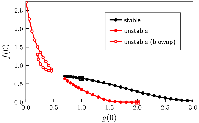
By looking at Fig. 1, one can observe several interesting features. The first is the existence of both stable and unstable branches in the space of gauged Q-ball solutions. By direct comparison with previous work, one can see that the regions of stability and instability correspond exactly with what has been found for axisymmetric perturbations (c.f. Fig. 3 of [10]). This suggests that three-dimensional perturbations do not excite any additional unstable modes for gauged Q-balls with in the logarithmic model. The appearance of a stable branch also addresses the general question of gauged Q-ball stability which was originally posed in [14] (namely, whether the Coulomb force will eventually destroy any gauged Q-ball when symmetry assumptions are relaxed). This reaffirms the possibility of gauged Q-balls as viable physical objects in realistic three-dimensional settings.
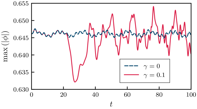
Let us discuss in further detail the behaviour of these stable configurations. As previously stated, we perturb each configuration in two ways: first, by the implosion of the field , and second, by truncation errors. In both cases, we find that the Q-balls respond to the perturbations by oscillating continuously around the equilibrium configurations. An illustration of this behaviour is given in Fig. 2. Initially, the gauged Q-ball remains at the origin and is perturbed only by truncation error. At , the field suddenly implodes through the origin. For the case where , this pulse interacts with the Q-ball and induces relatively large oscillations in the scalar field modulus which slightly distort the Q-ball profile. Additionally, the asymmetry of the imploding pulse imparts a small momentum “kick” to the Q-ball which sets it drifting away from the origin very slowly. However, for the case of , the imploding pulse has no effect on the Q-ball and it remains stationary. By continuing the evolution until , we observe that these general behaviours continue indefinitely—there is no significant change to the oscillatory pattern in either case. We therefore conclude that the corresponding solutions are stable.
Turning next to the unstable configurations in Fig. 1, we observe two disconnected branches with distinct behaviour. On the leftmost branch in the figure (labelled “blowup” and marked by red open circles), we find that the evolutions quickly become singular as the scalar field grows without bound in response to the perturbations. As described in [10], this behaviour can reasonably be attributed to the potential (5) being unbounded from below. In particular, it may become energetically favourable for the scalar field modulus to increase as the perturbations drive the field to a state of minimal . However, since there is no lower bound on for large , the energy density can become locally negative and the growth can continue indefinitely in a runaway effect. Since the resulting configurations do not retain any resemblance to the initial Q-ball, we classify them as unstable. We note that similar behaviour has also been observed in other Q-ball models which can attain negative energy densities [23, 24].
On the rightmost unstable branch of Fig. 1 (marked by red solid circles), we observe that the gauged Q-balls are quickly destroyed in response to the perturbations and can evolve in several ways. The most common outcome is the fragmentation of the original Q-ball into several smaller components. As an illustrative example, we plot in Fig. 3 the evolution of a gauged Q-ball which corresponds to configuration B in Table 1. This configuration is noteworthy in that it represents a shell-like concentration of the fields (a “gauged Q-shell” [13]) at the initial time. As the evolution proceeds, we observe that the Q-shell eventually breaks apart into six main components which travel coincident with the coordinate axes. We note that this instability, along with every other instability on the unstable branches of Fig. 1, can manifest quickly even without the influence of the perturbing field (i.e., with ). However, the specific manner in which the Q-ball breaks apart will depend on the configuration under study.
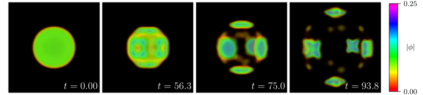
One notable feature of the evolution depicted in Fig. 3 is the absence of any ring-like structures (“gauged Q-rings”) after the Q-shell has broken apart. For the equivalent evolution in axisymmetry (see Fig. 7 of [10]), it has been reported that this particular configuration can result in the formation of gauged Q-rings which survive for some time. However, the absence of such structures in Fig. 3 suggests that the creation of Q-rings may be suppressed in full 3D. While we have still observed the formation of rings in other cases, we find that they are rare and usually break apart into smaller gauged Q-balls shortly after they appear. This indicates that long-lived gauged Q-rings may be considerably less common in three spatial dimensions (at least, for the type of evolutions and perturbations described here).
Next, we consider gauged Q-ball stability for the polynomial potential (6) with . Once again, we begin the analysis by applying the shooting procedure of Sec. III.1 to find gauged Q-ball configurations in the model. The space of solutions for this case is shown in Fig. 4. As stated previously, the choice is near the maximum allowable for the polynomial potential and no gauged Q-balls can be found with [21]. This significantly limits the range of possible solutions at large gauge coupling. Similar to the case of the logarithmic model, we evolve each configuration in Fig. 4 twice (once with and once with ) up to at least in order to assess the stability. Notably, we find no evidence for configurations which are unstable with respect to three-dimensional perturbations. This agrees with what has previously been reported for the equivalent evolutions in axisymmetry [10].
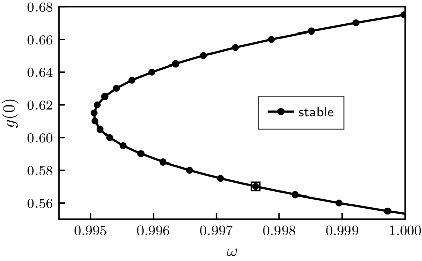
To conclude this section, let us examine the stability of gauged Q-balls for the polynomial potential (6) with . In this case, the gauge coupling is much smaller than what has been considered above and the space of possible solutions is correspondingly larger. We previously examined this scenario in axisymmetry [10] and found that the transition points between stability and instability in the solution space match closely with the transition points predicted for non-gauged Q-balls with . However, it was also noted that some solutions near the transition point exhibit “large oscillations in the Q-ball interior which significantly disrupt the shape of the configuration but do not cause the Q-ball to immediately break apart”. Since these solutions could not definitively be said to retain their initial shape, they were classified as unstable. Moreover, the recent results of [15] suggest a discrepancy between the transition point predicted by analytical calculations and the transition point identified numerically in [10]. Motivated by these factors, we now revisit this scenario and examine the same phenomenon using our fully three-dimensional code.
In Fig. 5, we plot the space of solutions for gauged Q-balls in the polynomial model (6) with . The curve can be broken down into three branches: an upper unstable branch I, a stable branch II, and a lower unstable branch III. Notably, the lower part of branch II and all of branch III are characterized by scalar field profiles which are step function-like and resemble the thin-wall Q-balls [25]. Once again, we perturb each configuration twice by setting and . Any gauged Q-balls which are clearly destroyed in response to either perturbation are classified as unstable while those which oscillate weakly or return toward the original configuration are classified as stable. For the solutions along branch I, we also observe that the Q-balls appear to collapse into solutions which lie along the stable branch II; we also classify these as unstable, though we comment that this behaviour makes it somewhat difficult to precisely identify the onset of instability. The salient feature of Fig. 5 in comparison to Fig. 12 of [10] is the different location for the transition point between branches II and III of the figure. In particular, this transition point is found to occur at a larger value of in three spatial dimensions and the “large oscillations” observed in axisymmetry are altogether absent. To verify this claim further, we have evolved the configurations with in Fig. 5 up to at least . Since the 3D simulations are expected to fully capture all unstable modes which would arise under axisymmetry assumptions, we conclude that this is a distinct result from what was reported in [10].
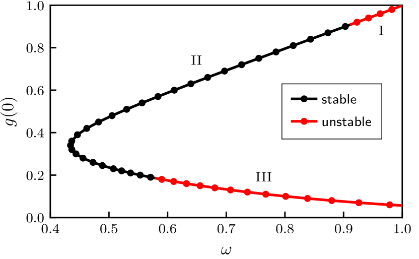
The origin of the “large oscillations” observed in axisymmetry is therefore puzzling, though it might reasonably be attributed to the unique numerical challenge of evolving the gauged Q-balls which lie along the lower part of branch II and branch III. In particular, the large thin-wall shape of these solutions results in sharp field gradients arising near the edge of the Q-ball. This can make it difficult to smoothly resolve the Q-ball boundary unless significant computational resources are expended. At the same time, we find that the instabilities of the Q-balls along this branch may only definitively manifest after several thousand time steps. This contrasts what is observed for other unstable gauged Q-balls in the logarithmic and polynomial models where the instabilities become obvious rather quickly. Together, these factors might result in the accumulation of numerical errors at late times which obscure the stability picture. For example, the oscillations observed in axisymmetry might possibly be due to a “de-phasing” of the periodic parts (real and imaginary) of the complex scalar field which eventually build up and disfigure the Q-ball profile. However, the fourth-order finite-difference scheme used in the present work is of a higher accuracy than the second-order method used in [10], so this may explain why such numerical artefacts are not observed here. Alternatively, the oscillations observed in axisymmetry may arise due to the different boundary conditions used or due to problems with the regularity of the evolved fields along the axis of symmetry at late times. In any case, the results of Fig. 5 suggest that the location of the instability threshold for these gauged Q-balls does not correspond so nearly with the prediction made by the stability criterion [26]. This contrasts what was previously reported in [10] but appears to agree with recent analytical findings [15].
IV.2 Collisions
We now consider relativistic collisions of gauged Q-balls in three spatial dimensions. To construct the binary system, we use the procedure described in Sec. III.1. The Q-balls are initialized at with initial velocities in the range . Additionally, we define the impact parameter as the linear distance between the center of the each Q-ball in the plane perpendicular to the initial motion. In our evolutions, we also test the effects of the relative phase difference and the relative sign of the Noether charge on the outcome of the collision. The phase difference is defined through a modification of the basic Q-ball ansatz (11),
| (27) |
By adjusting for one Q-ball in the binary, a relative difference in phase can be introduced into the system. This phase difference is preserved until the moment of impact for collisions of Q-balls with identical . Additionally, adjusting the parameter (while also taking in (12)) for one Q-ball in the binary can flip the overall sign of its Noether charge . In this manner, the dynamics of Q-ball/anti-Q-ball collisions can be investigated.
For all results presented below, we restrict our analysis to collisions involving configurations A and C in Table 1. Since configuration A is identical to configuration LogC in [11], and since configuration C is identical to configuration PolyB in [11], this enables a direct comparison between the collision dynamics in axisymmetry and the equivalent dynamics in three spatial dimensions. To facilitate this comparison, we have performed a number of head-on collision simulations of gauged Q-balls in 3D; we find the dynamics of these collisions to be broadly consistent with the axisymmetric case. In the discussion below, we will briefly review these results before turning to collision scenarios with non-zero impact parameter (which are unique to 3D).
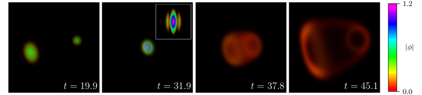
We first discuss the effects of the initial velocity on the outcome of head-on collisions with equal charge. For both A and C in Table 1, we find that the Coulomb repulsion of the gauged Q-balls can prevent any significant overlap of their respective scalar field content at low collision velocities. Instead, the Q-balls travel toward each other, reach a turning point of vanishing speed and then propagate back toward the boundaries. This occurs for for configuration A and for configuration C. At higher velocities, the gauged Q-balls are able to overcome their mutual repulsion and can behave in several different ways. For configuration A, we find that the outcome is typically a fragmentation of the gauged Q-balls into several smaller components. In most cases, a significant fraction of each original Q-ball continues to travel along the -axis after the collision. This is usually accompanied by the formation of smaller field remnants which are left behind near the origin and may travel away in different directions. For the case of configuration C, we find that the equivalent collisions result in the merger of the gauged Q-balls along with the emission of significant field content in the form of outgoing waves. At the highest collision velocities (e.g., for configuration A and configuration C), an increasing fraction of the field content travels parallel to the -axis after the collision. As illustrated in Fig. 6, this is accompanied by the development of a destructive interference pattern in at the moment of impact as well as the formation of gauged Q-rings in the case of configuration A.
We now turn to head-on collisions of gauged Q-ball with phase differences and opposite charges. It is well-known that the introduction of a phase difference can induce charge transfer between colliding Q-balls [27]. Here we observe similar behaviour using as a sample value. As in [11], we find that the gauged Q-balls created during the charge transfer process will often fragment into smaller Q-balls or even create transient Q-rings. In the case of configuration C, we also find some examples where the gauged Q-balls created during the collision will almost completely dissipate. However, the rate of charge transfer is found to decrease as in both cases. For head-on collisions with opposite charges, we find that the Coulomb force (which is now attractive) can accelerate the gauged Q-balls prior to the moment of impact. After the collision, the total Noether charge in the system is reduced as the Q-balls have partially annihilated. This process can create smaller Q-ball remnants which lag the main Q-balls (which are now highly perturbed) and propagate along or away from the -axis. It can also produce a wake of scalar radiation or a quasispherical pulse of electromagnetic radiation which emanates from the origin. In general, we find that the amount of charge which is annihilated depends on the collision velocity, with the least amount of annihilation occurring at the largest velocities.
While the above results are broadly consistent with the equivalent calculations in axisymmetry [11], we comment here on some subtle differences. One main difference relates to the behaviour of any gauged Q-rings which are created during the collisions. In axisymmetry, Q-rings were found to be a rather common outcome of intermediate- and high-velocity collisions that resulted in gauged Q-ball fragmentation. In these cases, the rings tended to propagate some distance away from the origin before collapsing back onto the axis of symmetry at late times (though this final fate could not be confirmed in all cases). While we have still observed the formation of gauged Q-rings in our fully three-dimensional simulations, we find that they tend to quickly break apart into a number of spherical gauged Q-balls in the majority of cases. It is only in rare circumstances (such as the scenario depicted in Fig. 6) where we have observed that the Q-rings can survive long enough to reach a radius which is many times greater than the size of the original Q-ball. This reaffirms our comments in Sec. IV.1 that Q-ring formation, while not explicitly forbidden, may be a rare phenomenon in the absence of symmetry restrictions.
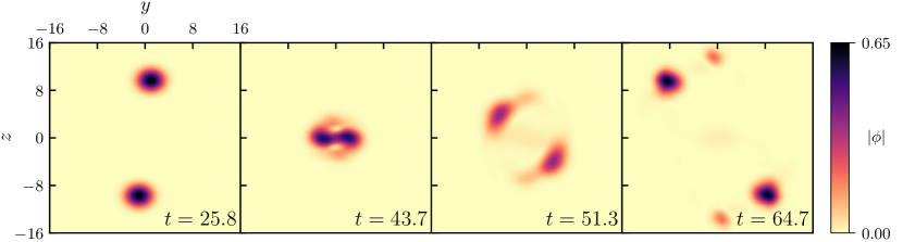
Having discussed the dynamics of head-on collisions, we now focus on the case where the impact parameter is non-zero. Since these “off-axis” collisions are obviously forbidden in axisymmetry, they represent a novel dynamical scenario which has not been explored in the previous studies. We begin by considering off-axis collisions of equal-charge gauged Q-balls. In this case, we find that a common outcome is the “deflection” of the gauged Q-balls due to the influence of the repulsive gauge field. This can result in the Q-balls following a discernible curved trajectory which makes an angle with the -axis at late times. The exact value of for a given collision can depend on several factors such as the initial velocity and the impact parameter . For equal-charge collisions, we find that is generally maximized when and are small (in fact, one could interpret the repulsive scenario discussed above for head-on collisions with equal charge and low velocity as a case of maximal deflection where ). However, when is sufficiently large and is not larger than the approximate Q-ball width, the scalar fields from each Q-ball can “graze” each other during the collision. In this case, the end result may be a fragmentation or merger of the gauged Q-balls. In Fig. 7, we plot a “grazing” collision of configuration A from Table 1 with equal charge, velocity , phase difference , and impact parameter . The gauged Q-balls collide at with a majority of the field content emerging at an angle with respect to the -axis. We also observe that the initial gauged Q-balls have partially fragmented into smaller objects which travel close to the -axis. Repeating the calculation shown in Fig. 7 for a variety of choices of and , we find that the outcomes are broadly consistent with what has been described above, though the deflection angles and fragmentation products may differ depending on the specific collision parameters.
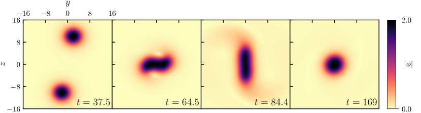
In Fig. 8, we plot a collision involving configuration C from Table 1 with equal charge, velocity , phase difference , and impact parameter . In contrast to what is shown in Fig. 7 for configuration A, here we see that the end result is a merger of the original gauged Q-balls. During the merger process, a significant amount of field content is radiated away toward the boundaries in the form of aspherical waves. By (the last panel in the figure), the merged configuration has settled down into a single gauged Q-ball centered at the origin which remains slightly perturbed. The properties of this final merged state turn out to be similar in some ways to the properties of configuration C before the collision. For example, the scalar field attains a value of at the origin by while the oscillation frequency (which we determine by tracking the real part of the scalar field during the collision) is found to be in the merged state. This result might be expected for gauged Q-balls with in the potential (6) since the space of possible solutions is extremely small (see Fig. 4). For configuration C, we find that mergers are a common outcome for moderate values of the collision velocity and impact parameter. At larger values of and , the gauged Q-balls can avoid the merged state through (for example) deflection of the fields.
It is worthwhile to discuss the final state of Fig. 8 in greater detail. Due to the off-axis motion of the binary, the total angular momentum of the system is non-zero at the initial time. It is plausible that some of this angular momentum may be retained by the merged configuration at late times, potentially representing an object analogous to a spinning Q-ball [28, 29]. At a visual level, the elongated and “rotating” appearance of in the second and third panel of Fig. 8 may also seem to support this idea. However, there are several reasons why the final merged state is unlikely to represent a configuration of this type. First, we observe that the gauged Q-ball very quickly returns to a near-spherical shape by through the emission of significant field content toward the boundaries. However, field configurations with angular momentum are not expected to be spherically-symmetric and may also be characterized by the presence of nodes away from the center [28]. Second, we have explicitly computed the angular momentum tensor,
| (28) |
and found that the -component of the angular momentum, , is almost totally radiated away from the origin by . Since the angular momentum of a spinning Q-ball (at least, in the non-gauged case) is expected to be an integer multiple of the Noether charge , we conclude that mergers of this type are unlikely to represent the usual spinning structures. At the same time, we cannot rule out the possibility that some small amount of angular momentum will still be retained in the merged state even at later times. If so, the configuration might be analogous to the “slowly rotating” Q-balls recently proposed in [30].
Next we turn to off-axis collisions of gauged Q-balls with opposite charges. Unlike the repulsive behaviour seen for the equivalent collisions with equal charge, here we observe that the Q-balls experience an attractive acceleration which curves their trajectories toward the origin. If the impact parameter and initial velocity are sufficiently large, the Q-balls may pass by one another without any significant interaction between their respective scalar fields. This is similar to the “deflection” described above for the equal-charge collisions, though now the deflection occurs in the opposite direction (i.e., toward the other Q-ball in the binary rather than away from it). If the impact parameter is small, the Q-balls will generally experience a “grazing” collision which can result in several possible outcomes. Most commonly, the gauged Q-balls will partially annihilate and fragment into a number of smaller components (for the case of configuration A) or radiate a portion of the field content toward the boundaries (for the case of configuration C); this is similar to their behaviour during head-on collisions. In Fig. 9, we plot the Noether charge density for a grazing collision involving configuration A from Table 1 with initial velocity , phase difference , and impact parameter . During the collision, the Q-balls complete a partial orbit around each other before escaping along a trajectory which is roughly perpendicular to their initial motion. A number of positively- and negatively-charged remnants are also created during the collision in the vicinity of the origin. By , approximately half of the total charge in the system has been annihilated. The acceleration and annihilation of charges during this process can also result in the production of an electromagnetic radiation pulse. In Fig. 10, we plot the energy contained in the electromagnetic field,
| (29) |
where and are the electric and magnetic field vectors, respectively. By comparing Fig. 9 and Fig. 10, we can see that a pulse of outgoing energy is created in the electromagnetic field which does not correspond to any significant amount of charge. We interpret this as representing electromagnetic radiation. We find the production of electromagnetic radiation to be a general phenomenon associated with gauged Q-ball/anti-Q-ball collisions, though the exact amount of radiation produced may depend on both the motion of the charges and the total amount of annihilation which occurs in the system.


To conclude this section, let us comment briefly on the off-axis collision of gauged Q-balls with a phase difference of . Similar to the case of head-on collisions, we find that the introduction of a relative phase difference can result in the transfer of charge between the colliding Q-balls. When the impact parameter is non-zero, the dynamics of this charge transfer can be altered in minor ways. For example, the charge transfer may occur asymmetrically such that the resulting Q-balls are left travelling at an angle relative to their initial motion; this angle can depend on both the collision velocity and the impact parameter. As the impact parameter is further increased, the amount of charge transfer appears to be reduced due to the smaller surface of contact between the colliding Q-balls. Otherwise, the charge transfer during off-axis collisions can generally be said to resemble the results for head-on collisions (including phenomena such as fragmentation or dissipation of the resulting Q-balls).
V Conclusion
In this work, we have studied the dynamical behaviour of gauged Q-balls using fully three-dimensional numerical evolutions. First, we investigated the classical stability of gauged Q-balls with respect to generic three-dimensional perturbations. Second, we explored the dynamics of gauged Q-balls during head-on and off-axis collisions at relativistic velocities.
With regards to stability, we have found numerical evidence for gauged Q-balls which remain stable against generic perturbations over long dynamical timescales. To reach this conclusion, we have perturbed the Q-balls in two different ways: through the inherent numerical error of our finite-difference implementation and through the interaction of an auxiliary scalar field which acts as a perturbing agent. Testing configurations in the logarithmic model, we have found evidence for both stable and unstable branches in the solution space. The solutions on the stable branch tend to respond to the perturbations by oscillating continuously near the initial configuration. The solutions on the unstable branch are found to break apart in various ways (usually into a number of smaller gauged Q-balls). We have also tested configurations in the sixth-order polynomial scalar field model, finding no evidence of unstable configurations for our choice of the model parameters with . Finally, we have revisited the case of in the polynomial model and found a new result for the transition point between stability and instability in the solution space. This result differs from what was found in [10] but appears to be in agreement with recent analytical findings [15].
With regards to relativistic collisions of gauged Q-balls, we have tested the effect of the initial velocity, relative phase, relative charge, and impact parameter on the outcome of the collision. For the case of head-on collisions, we have found that the dynamics in three spatial dimensions are broadly consistent with previous results reported under axisymmetry assumptions [11]. For the case of off-axis collisions, we have found that the impact parameter can play a significant role in modifying the collision outcome. For example, the gauged Q-balls can experience attractive or repulsive “deflections” from their initial trajectories depending on their relative charges, velocities, and the collision impact parameter. In other cases, the Q-balls may experience “grazing” collisions which can modify the dynamics during Q-ball fragmentation and mergers. Aside from these differences, the main phenomena associated with these collisions (such as charge transfer, annihilation, and radiation production) are found to be similar to the head-on case.
The results of this work are significant for several reasons. First, they address the general question of gauged Q-ball classical stability which was originally raised in [14]. Second, they provide new insights into the time-dependent behaviour of gauged Q-balls in realistic three-dimensional settings. Together, these results may be relevant for future studies of Q-balls in various physical contexts (such as in early-Universe cosmology). At the same time, we hope that this work may inspire further numerical explorations of related soliton models such as Proca Q-balls [31], spinning Q-balls [28, 29, 30], and charge-swapping Q-balls [32, 33, 34].
Acknowledgements.
This work was supported by the Natural Sciences and Engineering Research Council of Canada. Computing resources were provided by the Digital Research Alliance of Canada and the University of British Columbia.Appendix A Evolution Equations in Three Spatial Dimensions
When expressed using the coordinates defined by (7), the evolution equations for the system (2)–(3) take on the following form:
| (30) | ||||
| (31) | ||||
| (32) | ||||
| (33) | ||||
| (34) | ||||
| (35) |
Here, the subscripts correspond to the spacetime coordinates while the subscripts denote the real and imaginary parts of the scalar field, respectively. In deriving (30)–(35), we have invoked the Lorenz gauge condition (8) as a means to simplify the equations. After applying the coordinate transformations (24)–(26), we solve these equations using the fourth-order finite-difference scheme described in Sec. III.3 together with the initial data procedure of Sec. III.1.
Appendix B Code Validation
In order to assess the validity of our code, we have performed a series of numerical tests of convergence. In these tests, we use generic Gaussian-like initial data which approximately satisfies the constraint equations (9)–(10) at the initial time. We evolve the data on a uniform grid at various resolutions and compute the convergence factor as
| (36) |
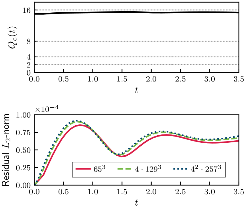
Here, represents the spacing between grid points, represents the solution computed with grid spacing , and denotes the -norm. For a finite-difference scheme with accuracy, one expects to find as [35]. We therefore expect to observe for the fourth-order finite-difference scheme described in Sec. III.3. In the top panel of Fig. 11, we plot the results of this test for the real part of the scalar field, , computed in the polynomial model (6) with , , and . Using grid resolutions of , , and to compute in (36), we find that the implementation is convergent to approximately fourth-order, as we expect. In addition to , we have also repeated this test for all other evolved quantities in the equations of motion (30)–(35). We find similar fourth-order behaviour in each case.
As a secondary test, we have performed an independent residual evaluation [35] to verify that our numerical solution reasonably approximates the continuum solution of the problem. In this test, the solution obtained using our fourth-order finite-difference scheme is substituted into a separate second-order centered discretization of the equations of motion (30)–(35). If the residuals of the these equations converge away at second-order in the grid spacing (corresponding to rescaling by factors of four), we conclude that the original finite-difference scheme has been correctly implemented. The results of this test are shown in the bottom panel of Fig. 11. Once again, we use grid resolutions of , , and and pick equation (30) as a representative example. In the figure, we observe the expected converge of the residual at second-order; the residuals for the other evolution equations (31)–(35) are found to behave in a similar way. This provides an additional check of the validity of our implementation.
References
- Coleman [1985] S. Coleman, Nucl. Phys. B262, 263 (1985).
- Coleman [1986] S. Coleman, Nucl. Phys. B269, 744 (1986).
- Kusenko and Shaposhnikov [1998] A. Kusenko and M. Shaposhnikov, Phys. Lett. B 418, 46 (1998).
- Kusenko and Steinhardt [2001] A. Kusenko and P. J. Steinhardt, Phys. Rev. Lett. 87, 141301 (2001).
- Enqvist and Laine [2003] K. Enqvist and M. Laine, J. Cosmol. Astropart. Phys. 08 (2003), 003.
- Bunkov and Volovik [2007] Y. M. Bunkov and G. E. Volovik, Phys. Rev. Lett. 98, 265302 (2007).
- Lee et al. [1989] K. Lee, J. A. Stein-Schabes, R. Watkins, and L. M. Widrow, Phys. Rev. D 39, 1665 (1989).
- Tamaki and Sakai [2014] T. Tamaki and N. Sakai, Phys. Rev. D 90, 085022 (2014).
- Gulamov et al. [2015] I. E. Gulamov, E. Y. Nugaev, A. G. Panin, and M. N. Smolyakov, Phys. Rev. D 92, 045011 (2015).
- Kinach and Choptuik [2023] M. P. Kinach and M. W. Choptuik, Phys. Rev. D 107, 035022 (2023).
- Kinach and Choptuik [2024] M. P. Kinach and M. W. Choptuik, Phys. Rev. D 110, 015012 (2024).
- Arodź and Lis [2009] H. Arodź and J. Lis, Phys. Rev. D 79, 045002 (2009).
- Heeck et al. [2021a] J. Heeck, A. Rajaraman, and C. B. Verhaaren, Phys. Rev. D 104, 016030 (2021a).
- Panin and Smolyakov [2017] A. G. Panin and M. N. Smolyakov, Phys. Rev. D 95, 065006 (2017).
- [15] A. Rajaraman, arXiv:2406.02817 [hep-th] .
- Press et al. [2007] W. H. Press, S. A. Teukolsky, W. T. Vetterling, and B. P. Flannery, Numerical Recipes: The Art of Scientific Computing, 3rd ed. (Cambridge University Press, Cambridge, England, 2007).
- Trottenberg et al. [2000] U. Trottenberg, C. W. Oosterlee, and A. Schüller, Multigrid, 1st ed. (Academic Press, San Diego, CA, United States, 2000).
- York Jr. and Piran [1982] J. W. York Jr. and T. Piran, in Spacetime and Geometry: The Alfred Schild Lectures, edited by R. A. Matzner and L. C. Shepley (University of Texas Press, Austin, TX, United States, 1982).
- Akbarian Kaljahi [2015] A. Akbarian Kaljahi, Numerical Studies in Gravitational Collapse, Ph.D. thesis, University of British Columbia (2015).
- Pretorius and Choptuik [2006] F. Pretorius and M. W. Choptuik, J. Comput. Phys. 218, 246 (2006).
- Loginov and Gauzshtein [2020] A. Y. Loginov and V. V. Gauzshtein, Phys. Rev. D 102, 025010 (2020).
- Radia et al. [2022] M. Radia, U. Sperhake, A. Drew, K. Clough, P. Figueras, E. A. Lim, J. L. Ripley, J. C. Aurrekoetxea, T. França, and T. Helfer, Class. Quantum Grav. 39, 135006 (2022).
- Anderson and Derrick [1970] D. L. T. Anderson and G. H. Derrick, J. Math. Phys. 11, 1336 (1970).
- Panin and Smolyakov [2019] A. G. Panin and M. N. Smolyakov, Eur. Phys. J. C 79, 150 (2019).
- Heeck et al. [2021b] J. Heeck, A. Rajaraman, R. Riley, and C. B. Verhaaren, Phys. Rev. D 103, 045008 (2021b).
- Correia and Schmidt [2001] F. P. Correia and M. Schmidt, Eur. Phys. J. C 21, 181 (2001).
- Battye and Sutcliffe [2000] R. A. Battye and P. M. Sutcliffe, Nucl. Phys. B590, 329 (2000).
- Volkov and Wöhnert [2002] M. S. Volkov and E. Wöhnert, Phys. Rev. D 66, 085003 (2002).
- Campanelli and Ruggieri [2009] L. Campanelli and M. Ruggieri, Phys. Rev. D 80, 036006 (2009).
- Almumin et al. [2024] Y. Almumin, J. Heeck, A. Rajaraman, and C. B. Verhaaren, Eur. Phys. J. C 84, 364 (2024).
- Heeck et al. [2021c] J. Heeck, A. Rajaraman, R. Riley, and C. B. Verhaaren, J. High Energy Phys. 10 (2021), 103.
- Copeland et al. [2014] E. J. Copeland, P. M. Saffin, and S.-Y. Zhou, Phys. Rev. Lett. 113, 231603 (2014).
- Xie et al. [2021] Q.-X. Xie, P. M. Saffin, and S.-Y. Zhou, J. High Energy Phys. 07 (2021), 062.
- Hou et al. [2022] S.-Y. Hou, P. M. Saffin, Q.-X. Xie, and S.-Y. Zhou, J. High Energy Phys. 07 (2022), 060.
- Choptuik [2006] M. Choptuik, Lectures for VII Mexican School on Gravitation and Mathematical Physics, http://laplace.physics.ubc.ca/People/matt/Teaching/06Mexico/mexico06.pdf (2006).