Variant Specific Treatment Effects with Applications in Vaccine Studies
Abstract.
Pathogens usually exist in heterogeneous variants, like subtypes and strains. Quantifying treatment effects on the different variants is important for guiding prevention policies and treatment development. Here we ground analyses of variant-specific effects on a formal framework for causal inference. This allows us to clarify the interpretation of existing methods and define new estimands. Unlike most of the existing literature, we explicitly consider the (realistic) setting with interference in the target population: even if individuals can be sensibly perceived as iid in randomized trial data, there will often be interference in the target population where treatments, like vaccines, are rolled out. Thus, one of our contributions is to derive explicit conditions guaranteeing that commonly reported vaccine efficacy parameters quantify well-defined causal effects, also in the presence of interference. Furthermore, our results give alternative justifications for reporting estimands on the relative, rather than absolute, scale. We illustrate the findings with an analysis of a large HIV1 vaccine trial, where there is interest in distinguishing vaccine effects on viruses with different genome sequences.
Keywords: Competing variants; Sieve effect; Interference.
1. Introduction
Infectious diseases are severe threats to human health, and vaccination is one of the most successful strategies for preventing them. However, a characteristic of infectious agents is their heterogeneity and rapid change. One example is HIV (Gaschen et al., 2002; Barouch, 2008; Johnston & Fauci, 2008), which exists in two main types, both of which have different variants. The heterogeneity is a challenge for the development of treatments, such as vaccines, because the treatment effect often depends on the characteristics of the circulating strain of a pathogen, and the presence of strains varies over time. For example, many vaccines are designed to target particular genetic sequences. These vaccines might offer less protection towards, say, evolving pathogens with different sequences in the target regions.
To describe existing strategies for quantifying treatment effects on heterogeneous variants, consider first a randomized controlled trial (RCT) where participants are assigned to vaccine or placebo treatment. Suppose that pathogens from infected individuals in each arm were recorded (Rolland et al., 2011; Hertz et al., 2016; Ouattara et al., 2020), and the recordings showed that the genetic sequences of the infected individuals in the vaccine arm differed from those in the placebo arm. Such differences have been attributed to heterogeneity in the effects of the vaccine on different variants, called ”sieve effects” (not to be confused with sieve estimators). This heuristic approach might be used as a test of a null hypothesis of equality of effects across variants, see Appendix A. Nevertheless, this approach does not adequately quantify the protective effect of the treatment on the different variants, which arguably is of primary interest for decision-makers.
Alternatively, there exist statistical ”sieve” methods for differentiating treatment effects against different variants of a pathogen (Gilbert et al., 1998; Gilbert, 2001; Gilbert et al., 2008; Sun et al., 2009; Juraska & Gilbert, 2013; Benkeser et al., 2019; Yang et al., 2022). This literature builds on results from competing events in survival analysis (Gilbert, 2000): individuals are considered to be at risk of experiencing an infection with different ”competing” variants over time. These sieve analysis methods have, for example, been applied to study effects of vaccination against HIV (Rolland et al., 2012, 2011; Zolla-Pazner et al., 2014; Hertz et al., 2016), malaria (Neafsey et al., 2015; Ouattara et al., 2020) and SARS-CoV-2 (Rolland & Gilbert, 2021).
The sieve methods that consider parameters on the cumulative incidence scale (Gilbert, 2001; Gilbert et al., 2001, 2008; Sun et al., 2009; Rolland et al., 2012; Zolla-Pazner et al., 2014; Neafsey et al., 2015; Benkeser et al., 2019, 2020; Yang et al., 2022), can be endowed with a causal interpretation as total effects in iid settings (Robins & Greenland, 1992; Young et al., 2020). Nevertheless, the relevance of these parameters requires more justification in infectious disease settings, even in a blinded randomized trial with perfect adherence. Unlike the study of non-communicable diseases, the cumulative incidence of each strain often varies due to differences in the number of infected and immune individuals across the strains (Garnett et al., 1996). Furthermore, the prevalence of the strains changes rapidly over time. To guide practice, e.g., large scale vaccination programs, estimands should sensibly reflect, or be insensitive to, such changes. Finally, interference between units might be a small problem in a perfectly executed trial examining a vaccine that is not yet available for public use; the interactions between the trial participants will often be negligible, which seems to be the justification for the use of iid assumptions in major vaccine trials. Nevertheless, interference will most likely be a concern if a vaccine is rolled out in a larger target population. Thus, to make the trial results relevant to the future decision setting, we need to argue that the parameters estimated under iid assumptions from the trial quantify the effects of interest in the relevant target population.
In this article, we develop causal methodology for quantifying vaccine efficacy against different disease-causing variants. Using explicit causal theory and assumptions, we clarify when we can make meaning to statements such as the treatment has the same effect on different variants. Our results also resolve concerns regarding interference, which threatens the generalization of the trial results to the target population. We achieve this by considering parameters that are defined by conditioning or intervening on (a possibly unmeasured) exposure status. We further elaborate on the implications of interference in Appendix B.
In practice, results of vaccine trials are usually presented on the relative scale. Yet, absolute effects are arguably more relevant to practical decision-making in many settings (VanderWeele & Knol, 2014). Indeed, claims favoring the relative scale, such as the stronger heterogeneity of the risk difference, have been suggested to have inadequate evidence (Poole et al., 2015). Our results can serve as justification for the relative measures, supporting claims made in the literature (Tsiatis & Davidian, 2022; Huang et al., 2023); in infectious disease settings, we show that measures on the relative scale can be identified under assumptions that do not allow identification of measures on the additive scale. The relative measures will also have certain stability properties. Furthermore, we show that identification formulas of different causal effects on the relative scale are equal under explicit assumptions, whereas the corresponding effects on the additive scale are generally different. To fix ideas, consider a running example on HIV vaccination.
1.1. The ALVAC/AIDSVAX vaccine against HIV
The efficacy of the ALVAC/
AIDSVAX vaccine was assessed in the RV144 RCT (NCT00223080, Rerks-Ngarm et al. (2009)). Data were collected from 16,395 healthy men and women, aged between 18 and 30 years in Thailand, initiated in October 2003. Treatment recipients were tested for HIV1 infection and viremia at the end of the vaccination period, 6 months from baseline, and then every 6 months in the following 3 years. Individuals were followed until the onset of the infection or the end of the follow-up period. While the vaccine showed evidence for the prevention of the HIV1 infection with a vaccine efficacy of 31.2% (95% CI: 1.1%, 52.1%) in the modified intention-to-treat sample, the effect of the vaccine waned over time and, therefore was not granted licensure by the FDA.
Rolland et al. (2012) conducted a sub-analysis based on the genome sequences of 110 individuals and found that, depending on the match and the mismatch of the vaccine at the amino acid positions 169 and 181 respectively, of the HIV-1 envelope variable 2, the vaccine efficacy increased to 48% (95% CI: 18%, 66%) against viruses matched to the vaccine at position 169, and to 78% (95% CI: 35%, 93%) against viruses mismatched to the vaccine at position 181. This difference compared to the overall vaccine efficacy of 31.2% suggests the appearance of a sieve effect (Gilbert et al., 1998). However, we cannot immediately interpret these differences as being causal effects. For example, the observed differences in rates may be confounded by factors such as the number of previous infections, like-with-like mixing, or changes in public policy. Another issue is interference, which is likely to be present in a setting where the vaccine is broadly available.
2. Data Structure and preliminary assumptions
Consider data from a study where individuals were randomly assigned to treatment or placebo, denoted by or , respectively. Suppose that the individuals were drawn from a much larger super-population, such that interference between trial participants is negligible. Thus, we assume that individuals are iid in the experiment (but not necessarily in the target population), which is also an implicit default assumption in classical vaccine trials (Chang et al., 1997; Whitney et al., 2003; Buchbinder et al., 2008), see Appendix B for more details. To avoid clutter, we hereby omit the subscript on the random variables. Moreover, let denote the vector of measured baseline covariates. Our effect of interest is the effect of the treatment, possibly conditional on or under interventions on exposure. Thus, we intentionally distinguish between the terms treatment () and exposure to a variant , where encodes no exposure (), exposure to variant 1 (), exposure to variant 2 (), and denotes exposure to both variants during the follow-up period (e.g., 42 months). The causal estimands we will consider can be identified in a setting with more than two variants, but for notational simplicity, we consider only variant 1 and variant 2. The following assumption will be used in the first parts of the manuscript:
Assumption 1 (Unique exposure).
Assumption 1 states that exposure to both variants is a probability zero event, which implies that exposure to each variant is mutually exclusive. The plausibility of Assumption 1 depends on the context: when studying diseases with low prevalence and correspondingly low exposure rates, exposure to multiple variants in a given time interval will have a probability (close to) zero. Such an argument will justify the preliminary assumption of mutual exclusivity of exposures. Let denote the outcome of interest, say severe infection, where the encoding corresponds to the definition of : 0 is no infection, 1 is infection by variant 1, and 2 is infection by variant 2 by the end of the follow-up period. In the case of the event , we assume that only one of the outcomes can occur. Under Assumption 1, the mechanism of determining which of the three outcomes, , are realized when is left undefined.
In Section 6, we discuss the time-to-event setting when these variables are taken to be time-dependent, which also allows us to assess exposure to multiple variants over time. Consideration of the time-to-event setting requires more involved notation, which we introduce when needed.
3. Time-fixed estimands
| Notation | Name | Identification Assumptions | Estimand | Identifying formula |
| Average treatment effect ratio | 3 | |||
| Relative causal effect conditional on exposure | 1, 2, 3, 4, 5 | |||
| Time-fixed estimands | ||||
| Contrast conditional on specific exposure | 1, 3, 4, 5, 6 | |||
| Contrast conditional on exposure | 1, 3, 4 | |||
| Effect with intervened exposure | 1, 4, 5, S3, S5 | |||
| Effect of exposure under treatment | 1, 4, 5, S1, S2 | |||
| Time-to-event estimands | ||||
| Time-to-event contrast conditional on exposure | 1, 7, 8a | |||
| Challenge subtype effect | 7, 8, 9, 10, 11 | |||
Our aim is to quantify the effect of treatment , say a vaccine, on the risk of developing the outcome , encoding infection by different variants. One motivation is that such estimands can inform us about the differential effects on the different variants, which, in turn, can guide future vaccine policies and development. However, there are various ways of defining such effects, and these definitions have different practical implications. To clarify these differences, we will explicitly define effects in a formal causal framework, assuming that the data were generated according to a finest fully randomized causally interpretable structured tree graph (FFRCISTG) model (Robins, 1986; Richardson & Robins, 2013), which is a strictly weaker causal model compared to the non-parametric structural equation model with independent errors (NPSEM-IE) (Pearl, 2009). Let superscripts denote potential outcome variables. In particular, if the value of treatment is fixed to , then the potential outcome of the variable is denoted by . Equivalently, denotes the outcome of an individual, if possibly contrary to fact, they had been assigned to exposure , for .
We first define a conventional estimand used in trials for assessing the effect of the vaccine on the specific outcome, that is the (relative) average treatment effect ().
Definition 1 (Average treatment effect).
The relative vaccine efficacy is conventionally reported as in vaccine trials. While the is identifiable with iid assumptions from standard RCT data, the , estimated from a conventional vaccine trial, cannot be interpreted as an average effect in a target population where there is interference. This is a problem because, in many infectious disease settings, there will be interference as treatments of one individual can affect the outcomes of others, e.g., through herd immunity. This fact is rarely discussed in vaccine trials but poses a problem for the policy relevance of the parameters.
To address the challenges in interpreting the population-level , we will define new estimands that are insensitive to interference by conditioning or intervening on exposure to variants. The rationale is that interference in vaccine settings is mediated through exposure status: when it is known that an individual is exposed to an infectious agent, their outcome is independent of the vaccine or infectious status of other individuals. Informally, we have an iid data structure conditional on, or under interventions on, exposure, even in the target population where the vaccine is rolled out. We further consider inference on these effects, even if the exposure status of an individual is unmeasured.
3.1. Estimands conditional on exposure
Consider first the effect on the individuals who would be exposed to variant regardless of treatment.
Definition 2 (Principal stratum effect of the always-exposed).
This is a causal effect, in the sense that it contrasts average outcomes under different treatments in the same subpopulation of individuals. However, the subpopulation is defined by counterfactual exposures under two different treatment assignments. Even in a hypothetical trial, such as a challenge trial, where the investigator observes the exposure status of the participants, the conditioning set cannot be identified without relying on additional untestable assumptions. Suppose, however, that the treatment does not affect the exposure (Stensrud & Smith, 2023), which is plausible in successfully blinded randomized experiments:
Assumption 2 (No effect on exposure).
It follows from Assumption 2 that . Therefore, the causal contrast in Definition 2 can be defined on the population of individuals who were observed to be exposed, as . Assumption 2 is analogous to assumptions imposed by, e.g., Greenwood & Yule (1915) and Halloran et al. (2010), positing that the exposure to the infectious agent should be the same for individuals, regardless of their inoculation status. Despite being of importance (Stensrud et al., 2024; Obolski et al., 2024), Assumption 2 is often only implicitly supposed in practical studies (Walsh et al., 2024).
Assumption 2 motivates the relative casual effect conditional on exposure (relative ), similarly to Stensrud & Smith (2023), but here we generalize this contrast to the multiple variant setting.
Definition 3 (Variant specific relative ).
Remark 1.
The ratio between relative for quantifies heterogeneity:
Definition 4 (Contrast conditional on subtype-specific exposure).
The is a measure of the relative effect of the treatment on the outcome, among those who were exposed to the specific subtype corresponding to the outcome. The contrast compares protection against variant 1 relative to variant 2, by examining those who were exposed to variants 1 and 2, respectively. This also means that the compares two relative s that are defined in distinct populations: those who were exposed to variant 1 vs those who were exposed to variant 2. The individuals exposed to variants 1 and 2 might have different characteristics, complicating the interpretation of the , as we discuss in more detail in Section 5.
Consider a different estimand, where we instead condition on :
Definition 5 (Contrast conditional on exposure).
Analogous to the , the measures the relative effect of the treatment on the two competing variants. However, the contrast is now defined among the exposed, without specifying the exact variant. If Assumption 2 holds, then the two conditioning sets are equal, allowing for a causal interpretation of the contrast. Even under a less restrictive assumption than Assumption 2, , the has a causal interpretation as a contrast of outcomes in the same population of individuals.
3.2. Estimands under interventions on exposure
Causal effects on different variants can also be defined via interventions on both the treatment and the exposure, i.e., with respect to the potential outcome . These effects correspond to contrasts identified in a challenge trial (Lambkin-Williams et al., 2018), where participants are exposed to the infectious pathogens in a controlled manner. Because we will consider these estimands conditional on baseline covariates , we will first include in the definitions.
Definition 6 (Effect with intervened exposure).
The , and the compare relative effect in the treated versus the untreated. We could also define a comparative estimand with respect to outcomes in the treated only:
Definition 7 (Effect of exposure under treatment).
When we generically discuss and , we will omit the argument whenever it is implied by the context.
The various definitions of the causal contrasts illustrate that there is no unique way of quantifying heterogeneous (sieve) effects. Instead, investigators should ask themselves, what is the relevant definition of heterogeneity in their context, and choose the effect measure accordingly, as we further discuss in Subsection 5. Furthermore, the investigators need to evaluate the assumptions needed to identify and estimate the estimands, as we described next (see also Table 1 for an overview).
4. Identification of the causal estimands
4.1. Identification of the
We first consider sufficient assumptions for the identification of the . We invoke conventional exchangeability, positivity, and consistency assumptions, which can be ensured by design in a classical RCT.
Assumption 3.
-
3a
Exchangeability:
-
3b
Positivity:
-
3c
Consistency:
While Assumption 3 is sufficient to identify the average treatment effect, , from the observed data, the relative of variants 1 and 2 require conditioning on exposure . If the exposure status of individuals is known, the can be expressed as a functional of the observed variables under Assumptions 1, 2 and 3. However, except for challenge trials, exposure status is usually unobserved in experiments. To identify the , we will introduce an additional assumption of exposure necessity.
Assumption 4 (Exposure necessity).
Assumption 4 guarantees that those who were not exposed to the infectious agent, will not develop either of the outcomes. In the running example on HIV, this means that individuals who were not exposed to either the matched or the unmatched variant, did not develop HIV infection. Because we consider different variants, we invoke an assumption guaranteeing that infection by either variant can only occur if individuals are exposed to that variant.
Assumption 5 (No cross-infectivity).
Assumption 5 allows the identification of the relative :
4.2. Identification of the and the
It follows from Proposition 1 that, under Assumptions 1-5, the and the can be identified
| (1) |
given that and . The proof of Proposition 1 and all the following identification proofs are given in Appendices C.1-C.12.
If the relative is identified for each , then the and the are identified. However, and the can also be identified under weaker assumptions, as presented next.
4.3. Relaxation of the identification conditions of the and the
Assumption 3 is standard in the causal inference literature and would hold by design in a randomized experiment with iid data. Here we will consider relaxations of Assumptions 2, 4, and 5. These relaxations will allow identification of the and the , even if the is unidentified.
4.3.1. No effect on exposure
Assumption 2 requires that . Consider the following weaker assumption:
Assumption 6 (No relative effect on exposure).
Assumption 6 states that the relative ratio between the exposures to variant 1 and variant 2 does not change with the assigned treatment. Under Assumption 3, Assumption 6 can be equivalently formulated as
In particular, Assumption 6 does not require successful blinding as, e.g., assumed by Stensrud & Smith (2023). Successful blinding is likely to be broken, e.g., when individuals more carefully adhere to protective behaviors under no treatment compared to vaccine assignment. The relaxed assumption would allow for such behaviors so long as the relative risk of exposure is constant across the two variants. This assumption could be plausible, e.g., when unvaccinated individuals reduce their number of social contacts and are careful about social distancing. Then the assigned treatment might influence the overall exposure levels, but likely not the ratio between the two variants.
4.3.2. Exposure necessity and No cross infectivity
Assumptions 4 and 5 guarantee that
where . Thus, Assumption 4 ensures that the identification formula for the defined in Table 1 not only identifies the ratio of the two s, but it is interpretable as the ratio of the expected potential outcomes, conditional on the non-zero status of the exposure.
If Assumption 5 further holds, then the same identification formula can be used to identify the ratio of the conditional outcomes under intervention conditional on the specific exposure that corresponds to the outcome.
4.4. Interpretation and identification of the and the
The and the require interventions on exposure, unlike the and the . Because the exposure in the and the is controlled, the ratio is insensitive to exposure patterns in the observed population. Therefore the estimated quantities can directly be generalized from a trial to the target population, as opposed to the conventional vaccine effect measures, that suffer from the confounding by the different interference structures. Both the and the can be identified in a challenge trial (Lambkin-Williams et al., 2018), where the exposure of the individuals to the infectious agents is controlled by the investigators. In practice, it is difficult to conduct such trials because of ethical considerations. Thus we focus on identifying the and the from standard RCT data which requires stronger assumptions. Sufficient conditions and identifying formulas are listed in Table 1, and these assumptions are described in more detail in Appendix E. Furthermore, we give results on and marginalized over in Appendices C.10 and C.12.
5. On the choice of estimand
The is identifiable from standard RCT data, without further assumptions, but its relevance to the target population is often questionable due to interference. The , , , and are defined by conditioning or intervening on the exposure of individuals (See Appendix B for details). Thus, these estimands are insensitive to interference in the target population. However, these four estimands have different interpretations and require additional assumptions for identification. Here we suggest more details on the choice of estimand, which is context-dependent.
5.1. and
The quantifies the ratio of relative treatment effect on each of the two competing variants ( vs ). In the context of the HIV1 example of Subsection 1.1, the compares the risk of infection with the matched variant () and the unmatched variant (), among those who were exposed to the matched () and the unmatched () variants, respectively. However, in general, would not necessarily mean that the vaccine has a more beneficial effect against one variant than the other because the conditioning sets differ; the individuals in the numerators and denominators might have different characteristics, which affect the risk of infection. Yet, we can conclude that the effect in the subpopulation of the exposed, , is different from the effect among the other subpopulation, .
In other words, the is not necessarily a causal effect, in the sense that it is defined by contrasting potential outcomes in different subpopulations, characterized by and . Assumption 2 ensures that . Assumption 1 states that being exposed to both of the variants has probability zero, hence there exists no subpopulation for which the four conditioning sets used in the are identical.
The is relevant when investigators are interested in whether the vaccine effects differ across subgroups of individuals, described by those exposed to exactly one of the two variants. In our running example on HIV, the identifying assumptions of the seem to be plausible. The short duration and the low prevalence of HIV justifies Assumption 1. Assumption 3 holds by design. Assumptions 4 and 5 are expected to hold, as without being in contact with the infectious agent, HIV cannot be developed, and the variant of exposure determines the type of outcome. The plausibility of Assumption 6 in RCTs even if blinding is broken is discussed in Subsection 4.3.1.
Unlike the , the is defined conditional on any exposure . This ensures that the numerator and denominator have the same conditioning sets. To fix ideas about the interpretation of the , consider the HIV1 trial, where the is the contrast of relative risks of infection with the two variants ( vs ) among those who were exposed to either variant . Under Assumption 5, individuals who developed outcome among the exposed () were exposed to variant . Indeed, Assumption 5 guarantees that the identification formulas for the and the are identical. The identifying assumptions for the are a strict superset of the ones that are sufficient for the identification of the .
Both the and the are estimands conditional on exposure, in the sense that they are defined in the subset of individuals who would be exposed in a given trial. This subset is context-dependent: it is possible that different people with different characteristics would be exposed at other times and locations. The context-dependence might threaten the generalizability of the and from the trial to the larger target population; the and would be equivalent in the target population if the characteristics of exposed individuals are exchangeable in the trial data and the target population.
In contrast, the and the are defined via an intervention on the exposure, that does not depend on the environment in which these estimands are estimated. However, the and the require stronger identification conditions compared to the and the , and their interpretations are different as well, which we discuss in the next subsections.
5.2.
To illustrate the relevance of the , consider two competing HIV1 variants that are present at distinct locations at a particular point in time. Suppose also that individuals at the two locations have different distributions of baseline covariates . In the future, however, it is likely that the variants will spread to different areas. A decision maker is interested in whether the vaccine effect differs across variants, potentially conditional on . The will give a concrete answer to this question.
The HIV1 example is not contrived, as different variants of various infectious agents are often present at different locations. For example, Castillo et al. (2020) discussed the geographical distribution of the variants of the SARS-CoV-2 in Chile. They found two regions where the proportion of variants was dominated by variant S, while in the rest of the regions, the most prevalent one was variant G. In the case of two available vaccines, with the possibly qualitatively different s with respect to these two variants, e.g., could have guided the distribution of these two hypothetical vaccines.
5.3.
Unlike the other estimands introduced so far, the only quantifies outcomes in vaccinated individuals (). Thus, the is particularly relevant when the vaccinated group is of special interest, like in settings where vaccination is compulsory. For example, yellow fever vaccination is required for visa applications to various countries.
The identification assumptions for both the and the require the measurement of baseline variables to adjust for unmeasured confounding between exposure (), treatment (), and outcome (). However, under certain assumptions (Assumptions 1, 4-6, S5 and with ), the can also be identified by the conventionally reported vaccine estimand, as defined in Equation (1). The could be identified with the same functional under Assumptions 1, 4-6, S1, S7 and with , see Appendix E.
Our considerations illustrate that the estimands have different interpretations and require different assumptions. We have given explicit assumptions ensuring that these (relative) estimands equal a conventional relative estimand. Had we considered estimands on the additive scale, then the same equalities would not in general hold, see Appendix J.
6. Time-to-event estimands
Many RCTs and observational studies produce longitudinal data, where events are recorded over time. Here we present time-to-event estimands and further extend the results from Section 4. The extensions are non-trivial, particularly because we need to consider (unmeasured) exposures and outcomes that vary over time.
6.1. Preliminaries
Let denote whether the individual was exposed to variant at time . In contrast, let indicate whether an individual has experienced the outcome by time , that is if the event has occurred at time or at any time , for . In particular, the exposure can change from time to . For example, an individual can be exposed to variant 1 at time , and then be exposed to variant 2, or be unexposed, at time , for . We also consider the further (and simpler) generalization to handle censoring in Appendix F. As we study the time to the first event in each individual, we arbitrarily set future exposures to zero after an event has occurred: formally for all .
Consistent with the conventional causal inference literature (Robins, 1997; Hernan & Robins, 2023), consider discrete time intervals , and the random variables indexed with negative subscripts are considered to be equal to 0. The history of the random variables, through the current interval , are denoted by an overline, for example, .
Let denote the common causes of the outcomes and the exposures, let denote the common cause of the outcomes only, and let denote the common cause of the exposures, as illustrated by the Single World Intervention Graph (SWIG) (Richardson & Robins, 2013) in Figure 1. Here, , and might be unmeasured.
To motivate the extension to multiple exposures over time, consider the HIV1 example and suppose that at time sufficient contact for infection was made between a susceptible () individual and someone infected by the matched variant (), e.g. needle sharing during injection drug use (Patel et al., 2014). It is plausible that a second sufficient contact follows at time , with someone who is infected by the unmatched strain ().
6.2. Challenge subtype effect
The challenge subtype effect quantifies the differential effect of the vaccine on the two competing variants in a setting where the exposure is administered at a particular time:
Definition 8 (Challenge subtype effect).
for all
The is insensitive to interference by, e.g., mixing patterns, as it is defined under (time-varying) interventions on exposure, . We also consider an additional time-to-event estimand in Appendix G, which can be conceptualized as a straight-forward extension of the time-fixed estimand to the time-to-event data.
7. Time-to-event identification
Consider the following assumptions, which generalize Assumption 3 and hold by design in a properly executed randomized trial.
Assumption 7.
-
7a
TTE Exchangeability:
-
7b
TTE Positivity:
-
7c
TTE Consistency:
Assumption 8 (TTE exposure necessity).
-
8a
-
8b
Under Assumption 8b, the history of non-exposure until time is independent of the outcome at time , given the exposure at time , the history of no outcome until time and the value of the possibly unmeasured variables and .
Assumption 9 (TTE no cross-infectivity).
Furthermore, consider the following assumption that describes how exposures to different variants are related.
Assumption 10 (Exposure ratio of the exposed).
for all , and , with being constant across the values and .
Assumption 10 guarantees that, among those exposed to any of the variants, the ratio of probabilities of being exposed to variant 1 and variant 2 is constant in and . For example, let the variables and represent age and urban vs non-urban residency respectively, both of which can be associated with the social activity of an individual. Suppose that socially active people have a higher chance of exposure compared to those who limit social interactions. Then we assume that both the socially active and inactive have the same relative rate of being exposed to variant 1 and variant 2. However, we do allow that the relative prevalence of the two variants might change over time and, thus, we also allow that the relative exposure ratios change with , see the Single World Intervention Graph (SWIG) in Figure 1 as an example, consistent with Assumptions 7-10. Assumption 10 can fail if either and are associated with geographical regions where variants appear with different prevalence (Castillo et al., 2020).
Proposition 3 gives an identification formula of the based on factual variables. However, and capture all common causes of the time-variant outcomes and exposures or outcomes only, that may, e.g., include social activity, age, sex, general health status, socio-economic status, and genetic factors. All of these factors are usually impossible to measure in an RCT. To identify the population , without measuring and , consider the following assumption.
Assumption 11 (Scaled new infection).
for all , and , where we define whenever
.
Assumption 11 is encoding a particular heterogeneity in infectivity on the ratio scale. This assumption will be plausible if the infectious pathways are similar for the two variants across all the subpopulations defined by the different values of and . A falsification test of Assumption 11, based on the observed subset of and , is presented in Appendix H.2.
Remark 4.
Assumption 11 can equivalently be formulated such that the conditioning set includes the history of the outcome variable under interventions and , until time ,
for all , and . Under the FFRCISTG model, factorizing according to the SWIG in Figure 1, Assumption 11 can be rewritten using minimal labeling as
The next corollary and proposition give convenient identification results for .
Using the equality between the marginal and the conditional s the marginal can be identified as a function of observed variables.
7.1. On testing of a null effect
Consider the sharp null hypothesis that the vaccine has the same effect on developing the two types of outcomes at time , under controlled exposure conditions:
| (3) | ||||||
Alternatively, consider the stronger sharp null hypothesis
| (4) |
Suppose that an individual had their first exposure at time . Suppose that this exposure led to infection with variant . Then, implies that, exposure to variant would lead to infection with variant . It is easy to show that
implies . The distinction between and can be illustrated by an individual with characteristics:
This individual is doomed if exposed to variant 1, but immune to variant 2, consistent with but not . Under Assumption 11, the potential outcome probabilities under different treatment interventions are related:
Proposition 5 (Proportionality under the null).
A practical implication of Proposition 5 is that by assuming proportional potential outcomes amongst the untreated, and Assumptions 7-10, under the null hypothesis , is identified as
| (5) |
Under the strong null hypothesis , we have that Assumption 11 holds, with the particular value of .
Lemma 1.
8. Testing and estimation
8.1. Time-fixed estimation
The identifying formulas in Table 1 are all ratios of estimable conditional probabilities. Denote the estimators for conditional probabilities and by and , respectively. Furthermore, let and be the estimators of and for all and , respectively. Suppose first that we have unbiased estimators of these quantities, for example, empirical means of indicator functions. Then, under Assumptions 3 the can be estimated by
However, the -s cannot be calculated in most practical settings because is unobserved. If we further impose Assumptions 4-6, then
is an asymptotically unbiased estimator of the . Estimators for the causal estimands in Table 1 follow analogously, and the corresponding estimators of the are denoted as and respectively. Estimated confidence intervals for the , the , and the are can, e.g., be derived using the log-normal approximation discussed by Katz et al. (1978), and for the the confidence intervals are calculated based on the work of Nelson (1972).
8.2. Time-to-event estimation
The identification formula of the marginal in Proposition 4 is a functional of two time-varying hazard ratios, one for each variant. These hazard ratios can, e.g., be estimated semi-parametrically using Cox regression (Cox, 1972), or non-parametrically by sample means of the event rates among the at risk population, see Appendix H for details.
Assumption 11 imposes strong proportionality conditions, conditional on the unobserved variables and . Let us consider a subset of these two variables denoted as , that is observed by the investigators. Then under Assumptions 7-11,
for all . This equality can, e.g., be tested by inverting confidence intervals of the corresponding coefficients in two Cox proportional hazard models fitted to estimate the cause-specific hazards of outcomes with variant 1 and 2, respectively. Details are provided in Appendix H.2. The use of different estimators of the is further illustrated in Appendix H.1.
9. Effects of the ALVAC/AIDSVAX vaccine on HIV1 variants
We use publicly available data from Benkeser & Hejazi (2017) based on the RV144 trial that studied the effect of the ALVAC/AIDSVAX vaccine on the risk of HIV1 infection (Rerks-Ngarm et al., 2009), as described in Subsection 1.1. For data privacy reasons, our individual-level dataset is synthetically constructed to mimic the outcomes in the original trial (Benkeser & Hejazi, 2017). Participants received placebo () or active vaccine (). The outcome of interest is the presence of HIV infection matched () or mismatched () to the vaccine at the amino acid position 169. We also had access to categorical baseline covariates encoding year of the enrollment, sex, age, risk profile. In our analysis, we assumed uninformative censoring (Assumption S9, see Appendix F).
9.1. Time-fixed estimates
We estimated the to be ( CI: ) based on Method C described by Katz et al. (1978). Under the identification assumptions of the (Assumptions 1, 4, 5,S3, and S5), which we suppose to hold conditional on the baseline covariate risk profile, the is identified by the same functional as the in the High risk and Non-high risk populations. The corresponding estimates are ( CI: ) and ( CI: ), respectively. We estimated effects under alternative assumptions in Appendix E.4.
9.2. Time-to-event estimates
Based on the developments in Section 8, we estimated the marginal using two marginal Cox models, for the two subtypes respectively, where individuals were censored when they either experienced infection with the competing subtype or early drop-out (Young et al., 2020). That is,
where denotes the potential outcomes under no censoring, see for more details Appendix F. Under this model, the identification formula of the simplifies to , which was estimated to be , where the 95% confidence interval was estimated by non-parametric Bootstrap in 10,000 samples. Homogeneity in effects across strains corresponds to . Thus, we conclude that there is heterogeneity, i.e., variant-specific effects.
We also used the conventional Nelson-Aalen estimator (Aalen, 1978) to non-parametrically estimate the cumulative hazards of being infected with each variant. We can use these estimates to test a modified null hypothesis, as formally defined in Appendix H.2. The ratio of the cumulative hazards is estimated to be 0.230 (95% CI: [0, 0.613]), and 0.427 (95% CI: [0.000, 0.876]) in the first and the second half of the trial, respectively.
9.3. Remark on rare events
The estimated in a time-fixed setting is , and the estimated via Cox regression is , for all , while the cumulative hazard using the non-parametric Nelson-Aalen estimator at the end of the follow-up period is estimated to be . The similarity between the estimates is expected because of the small number of events; when events are rare, it is well-known that the hazard ratio approximates the risk ratio (Symons & Moore, 2002). For the details of alternative estimators of the sieve effect when events are rare, see Appendix H.3.
10. Discussion
We have formally defined various causal estimands that are relevant in studies of subtype-specific outcomes. Under explicit assumptions, we showed that the estimands can be identified by simple functionals in conventional RCTs. These formalizations clarify the interpretation of commonly estimated vaccine parameters used in large-scale randomized trials. It is practically important that our results can justify the use of conventional relative vaccine estimands, calculated under iid assumptions from RCT data, even if there is interference in the target populations. While we have given sufficient conditions for the identification of various estimands, alternative identification strategies might also be useful and plausible in certain settings. In future research, we will particularly study (sharp) bounds, i.e., partial identification under weaker identifiability assumptions.
References
- noa (2023) (2023). Volume 28, Number 3 | HIV Surveillance | Reports | Resource Library | HIV/AIDS | CDC.
- Aalen (1978) Aalen, O. (1978). Nonparametric Inference for a Family of Counting Processes. The Annals of Statistics 6, 701–726.
- Aronow (2012) Aronow, P. M. (2012). A General Method for Detecting Interference Between Units in Randomized Experiments. Sociological Methods & Research 41, 3–16.
- Barouch (2008) Barouch, D. H. (2008). Challenges in the development of an HIV-1 vaccine. Nature 455, 613–619.
- Benkeser et al. (2019) Benkeser, D., Gilbert, P. B., Carone, M. (2019). Estimating and Testing Vaccine Sieve Effects Using Machine Learning. Journal of the American Statistical Association 114, 1038–1049.
- Benkeser & Hejazi (2017) Benkeser, D., Hejazi, N. (2017). benkeser/survtmle: survtmle – first CRAN release.
- Benkeser et al. (2020) Benkeser, D., Juraska, M., Gilbert, P. B. (2020). Assessing trends in vaccine efficacy by pathogen genetic distance. Journal De La Societe Francaise De Statistique (2009) 161, 164–175.
- Buchbinder et al. (2008) Buchbinder, S. P., Mehrotra, D. V., Duerr, A. et al. (2008). Efficacy assessment of a cell-mediated immunity HIV-1 vaccine (the Step Study): a double-blind, randomised, placebo-controlled, test-of-concept trial. Lancet 372, 1881–1893.
- Castillo et al. (2020) Castillo, A. E., Parra, B., Tapia, P. et al. (2020). Geographical Distribution of Genetic Variants and Lineages of SARS-CoV-2 in Chile. Frontiers in Public Health 8, 562615.
- Chang et al. (1997) Chang, M.-H., Chen, C.-J., Lai, M.-S. et al. (1997). Universal Hepatitis B Vaccination in Taiwan and the Incidence of Hepatocellular Carcinoma in Children. New England Journal of Medicine 336, 1855–1859.
- Cox (1972) Cox, D. R. (1972). Regression Models and Life-Tables. Journal of the Royal Statistical Society. Series B (Methodological) 34, 187–220.
- Garnett et al. (1996) Garnett, G. P., Hughes, J. P., Anderson, R. M. et al. (1996). Sexual Mixing Patterns of Patients Attending Sexually Transmitted Diseases Clinics. Sexually Transmitted Diseases 23, 248–257.
- Gaschen et al. (2002) Gaschen, B., Taylor, J., Yusim, K. et al. (2002). Diversity Considerations in HIV-1 Vaccine Selection. Science 296, 2354–2360.
- Gilbert et al. (2001) Gilbert, P., Self, S., Rao, M. et al. (2001). Sieve analysis: methods for assessing from vaccine trial data how vaccine efficacy varies with genotypic and phenotypic pathogen variation. Journal of Clinical Epidemiology 54, 68–85.
- Gilbert (2000) Gilbert, P. B. (2000). Comparison of competing risks failure time methods and time-independent methods for assessing strain variations in vaccine protection. Statistics in Medicine 19, 3065–3086.
- Gilbert (2001) Gilbert, P. B. (2001). Interpretability and robustness of sieve analysis models for assessing HIV strain variations in vaccine efficacy. Statistics in Medicine 20, 263–279.
- Gilbert et al. (2008) Gilbert, P. B., McKeague, I. W., Sun, Y. (2008). The 2-sample problem for failure rates depending on a continuous mark: an application to vaccine efficacy. Biostatistics (Oxford, England) 9, 263–276.
- Gilbert et al. (1998) Gilbert, P. B., Self, S. G., Ashby, M. A. (1998). Statistical Methods for Assessing Differential Vaccine Protection Against Human Immunodeficiency Virus Types. Biometrics 54, 799–814.
- Greenwood & Yule (1915) Greenwood, Yule, G. U. (1915). The Statistics of Anti-Typhoid and Anti-Cholera Inoculations, and the Interpretation of Such Statistics in General. Proceedings of the Royal Society of Medicine 8, 113–194.
- Halloran et al. (2010) Halloran, M. E., Longini, I. M., Struchiner, C. J. (2010). Design and Analysis of Vaccine Studies. Statistics for Biology and Health. New York, NY: Springer New York.
- Hayes et al. (2000) Hayes, R. J., Alexander, N. D., Bennett, S. et al. (2000). Design and analysis issues in cluster-randomized trials of interventions against infectious diseases. Statistical Methods in Medical Research 9, 95–116.
- Hernan & Robins (2023) Hernan, M. A., Robins, J. M. (2023). Causal Inference: What If. CRC Press.
- Hertz et al. (2016) Hertz, T., Logan, M. G., Rolland, M. et al. (2016). A study of vaccine-induced immune pressure on breakthrough infections in the Phambili phase 2b HIV-1 vaccine efficacy trial. Vaccine 34, 5792–5801.
- Hu et al. (2022) Hu, Y., Li, S., Wager, S. (2022). Average direct and indirect causal effects under interference. Biometrika 109, 1165–1172.
- Huang et al. (2023) Huang, T.-J., Luedtke, A., THE AMP INVESTIGATOR GROUP (2023). Improved efficiency for cross-arm comparisons via platform designs. Biostatistics 24, 1106–1124.
- Johnston & Fauci (2008) Johnston, M. I., Fauci, A. S. (2008). An HIV Vaccine — Challenges and Prospects. New England Journal of Medicine 359, 888–890.
- Juraska & Gilbert (2013) Juraska, M., Gilbert, P. B. (2013). Mark-specific hazard ratio model with multivariate continuous marks: an application to vaccine efficacy. Biometrics 69, 328–337.
- Katz et al. (1978) Katz, D., Baptista, J., Azen, S. P. et al. (1978). Obtaining Confidence Intervals for the Risk Ratio in Cohort Studies. Biometrics 34, 469–474.
- Lambkin-Williams et al. (2018) Lambkin-Williams, R., Noulin, N., Mann, A. et al. (2018). The human viral challenge model: accelerating the evaluation of respiratory antivirals, vaccines and novel diagnostics. Respiratory Research 19, 123.
- Longini Jr. et al. (2002) Longini Jr., I. M., Halloran, M. E., Nizam, A. (2002). Model-based estimation of vaccine effects from community vaccine trials. Statistics in Medicine 21, 481–495.
- Neafsey et al. (2015) Neafsey, D. E., Juraska, M., Bedford, T. et al. (2015). Genetic Diversity and Protective Efficacy of the RTS,S/AS01 Malaria Vaccine. New England Journal of Medicine 373, 2025–2037.
- Nelson (1972) Nelson, W. (1972). Statistical Methods for the Ratio of Two Multinomial Proportions. The American Statistician 26, 22–27.
- Obolski et al. (2024) Obolski, U., Stensrud, M. J., Nevo, D. (2024). A call for blinding assessments in dengue vaccine trials. The Lancet Infectious Diseases 24, e10.
- Ouattara et al. (2020) Ouattara, A., Niangaly, A., Adams, M. et al. (2020). Epitope-based sieve analysis of plasmodium falciparum sequences from a fmp2.1/as02a vaccine trial is consistent with differential vaccine efficacy against immunologically relevant ama1 variants. Vaccine 38, 5700–5706.
- Patel et al. (2014) Patel, P., Borkowf, C. B., Brooks, J. T. et al. (2014). Estimating per-act HIV transmission risk: a systematic review. AIDS 28, 1509–1519.
- Pearl (2009) Pearl, J. (2009). Causality. Cambridge University Press.
- Poole et al. (2015) Poole, C., Shrier, I., VanderWeele, T. J. (2015). Is the Risk Difference Really a More Heterogeneous Measure? Epidemiology 26, 714.
- Rerks-Ngarm et al. (2009) Rerks-Ngarm, S., Pitisuttithum, P., Nitayaphan, S. et al. (2009). Vaccination with ALVAC and AIDSVAX to Prevent HIV-1 Infection in Thailand. New England Journal of Medicine 361, 2209–2220.
- Richardson & Robins (2013) Richardson, T. S., Robins, J. M. (2013). Single world intervention graphs (SWIGs): A unification of the counterfactual and graphical approaches to causality. Center for the Statistics and the Social Sciences, University of Washington Series. Working Paper 128, 2013.
- Robins (1986) Robins, J. (1986). A new approach to causal inference in mortality studies with a sustained exposure period—application to control of the healthy worker survivor effect. Mathematical modelling 7, 1393–1512.
- Robins (1997) Robins, J. M. (1997). Causal Inference from Complex Longitudinal Data. In Latent Variable Modeling and Applications to Causality, M. Berkane, ed. New York, NY: Springer.
- Robins & Greenland (1992) Robins, J. M., Greenland, S. (1992). Identifiability and Exchangeability for Direct and Indirect Effects. Epidemiology 3, 143–155.
- Rolland et al. (2012) Rolland, M., Edlefsen, P. T., Larsen, B. B. et al. (2012). Increased HIV-1 vaccine efficacy against viruses with genetic signatures in Env V2. Nature 490, 417–420.
- Rolland & Gilbert (2021) Rolland, M., Gilbert, P. B. (2021). Sieve analysis to understand how SARS-CoV-2 diversity can impact vaccine protection. PLOS Pathogens 17, e1009406.
- Rolland et al. (2011) Rolland, M., Tovanabutra, S., deCamp, A. C. et al. (2011). Genetic impact of vaccination on breakthrough HIV-1 sequences from the STEP trial. Nature Medicine 17, 366–371.
- Rosenbaum (2007) Rosenbaum, P. R. (2007). Interference between Units in Randomized Experiments. Journal of the American Statistical Association 102, 191–200.
- Stensrud et al. (2024) Stensrud, M. J., Nevo, D., Obolski, U. (2024). Distinguishing Immunologic and Behavioral Effects of Vaccination. Epidemiology 35, 154.
- Stensrud & Smith (2023) Stensrud, M. J., Smith, L. (2023). Identification of Vaccine Effects When Exposure Status Is Unknown. Epidemiology 34, 216–224.
- Sun et al. (2009) Sun, Y., Gilbert, P. B., McKeague, I. W. (2009). Proportional Hazards Models with Continuous Marks. The Annals of Statistics 37, 394–426.
- Symons & Moore (2002) Symons, M. J., Moore, D. T. (2002). Hazard rate ratio and prospective epidemiological studies. Journal of Clinical Epidemiology 55, 893–899.
- Sävje et al. (2021) Sävje, F., Aronow, P. M., Hudgens, M. G. (2021). Average treatment effects in the presence of unknown interference. The Annals of Statistics 49, 673–701.
- Tsiatis & Davidian (2022) Tsiatis, A. A., Davidian, M. (2022). Estimating vaccine efficacy over time after a randomized study is unblinded. Biometrics 78, 825–838.
- VanderWeele & Knol (2014) VanderWeele, T. J., Knol, M. J. (2014). A Tutorial on Interaction. Epidemiologic Methods 3.
- Walsh et al. (2024) Walsh, M.-C. R., Alam, M. S., Pierce, K. K. et al. (2024). Safety and durable immunogenicity of the TV005 tetravalent dengue vaccine, across serotypes and age groups, in dengue-endemic Bangladesh: a randomised, controlled trial. The Lancet Infectious Diseases 24, 150–160.
- Whitney et al. (2003) Whitney, C. G., Farley, M. M., Hadler, J. et al. (2003). Decline in Invasive Pneumococcal Disease after the Introduction of Protein–Polysaccharide Conjugate Vaccine. New England Journal of Medicine 348, 1737–1746.
- Yang et al. (2022) Yang, G., Balzer, L. B., Benkeser, D. (2022). Causal inference methods for vaccine sieve analysis with effect modification. Statistics in Medicine 41, 1513–1524.
- Young et al. (2020) Young, J. G., Stensrud, M. J., Tchetgen Tchetgen, E. J. et al. (2020). A causal framework for classical statistical estimands in failure‐time settings with competing events. Statistics in Medicine 39, 1199–1236.
- Zolla-Pazner et al. (2014) Zolla-Pazner, S., Edlefsen, P. T., Rolland, M. et al. (2014). Vaccine-induced Human Antibodies Specific for the Third Variable Region of HIV-1 gp120 Impose Immune Pressure on Infecting Viruses. eBioMedicine 1, 37–45.
Online Appendix
A. Concordance between notions of sieve effects
Assume that data were collected from a randomized clinical trial. Specifically, if an individual was affected by any outcome, , then the genetic distance from the infectious variant to the vaccine insert , was recorded.
Suppose that the outcome was classified as matched, , if the distance from the vaccine insert was less than a threshold value . Based on this threshold value, the distance variable can be dichotomized to , and the one-to-one relationship between the outcome and the discrete distance can be established as .
Using a statistical sieve effect approach (Gilbert et al., 1998; Gilbert, 2001; Gilbert et al., 2008; Sun et al., 2009; Juraska & Gilbert, 2013; Benkeser et al., 2019, 2020; Yang et al., 2022), see for example Table 1, the effect of the vaccine on the two variants would be contrasted, for instance by calculating the respective relative risks from a trial where is randomly assigned. That is,
The ratios of the dichotomized distances are contrasted between the treatment and the control arms, that is
In our setting, by definition, and there is a bijective map between these two contrasts.
B. Interference and vaccine trials
The assumption of no interference is often invoked in vaccine trials.
No interference implies that the potential outcomes of individuals are independent of the treatment received by other trial participants. More explicitly, for all and , where are the treatment assignments of all but the -th individual. The recurring reasoning in vaccine trials is that the infectious contacts made between the trial participants are negligible. Therefore the treatment of individual does not affect the outcome for any . This allows us to write , where . Following this argument, suppose that a vaccine trial is analyzed with conventional frequentist (superpopulation) methods under iid assumptions, in particular, no interference. Then we can interpret the results as valid for a hypothetical population where the no interference assumption holds, for example, a superpopulation of individuals that, say, are sparsely embedded in a larger population so that they do not interact.
Yet, decision-makers will frequently use the trial results to inform policies in populations where there is interference. In realistic target populations, the treatment assignments of one unit can affect outcomes of other units, often referred to as a spillover effect, or in the setting of vaccines against infectious diseases, as, e.g., herd immunity. It follows that, in this target population, the potential outcome is no longer well-defined because of interference; the assumption does not hold for every and , thus the potential outcomes cannot be defined at individual level interventions only. Thus, even if individuals are iid in an experiment, the use of conventional iid methods will not necessarily target estimands that are of broader policy interest.
A potential solution could be defining the causal effects in terms of interventions on the whole study population, for example as . However, identification and estimation of this quantity would not be possible from the conventional trial data, without imposing strong assumptions about the interference structure.
To consider another solution, suppose that the treatment assignment of units affects other units’ outcomes mediated through exposure. In specific, the single directed causal path between
and is . This structure is plausible when considering communicable infectious diseases, which precisely can spread from infectious to susceptible subjects. This is, e.g., reflected in conventional infectious disease models, although we emphasize that our causal structure is less restrictive than, say, SIR or SIER models.
By conditioning or intervening on the value of exposure to the infectious agent, there will be no dependence between the treatment of individual and outcome of individual . That is, for all and , such that for all , . Thus, when we condition or intervene on exposure, we can assume no interference between the potential outcomes of individuals in the realistic target population. This is one rationale for considering our target estimands that are explicitly defined with respect to exposure status.
Our work contributes to the existing rich literature on the statistical issue of interference (Rosenbaum, 2007; Aronow, 2012; Sävje et al., 2021; Hu et al., 2022). While some of these works study specifically vaccine effects as well (Hayes et al., 2000; Longini Jr. et al., 2002), we do not impose constraints on the interference structure, or consider special types of randomized designs. Our results are valid under the usual frequentist superpopulation framework, without considering design based inference, where the estimands are explicit functions of randomization probabilities.
C. Proofs
C.1. Proof of Proposition 1
C.2. Proof of Proposition 2
C.3. Proof of identification
C.4. Proof of Proposition 3
Proof.
First note that for all and
where for the second line we used laws of probability and Assumption 8a in both lines two and three. In the fourth line, we used Assumption 7a, while in the fifth line, we used Assumptions 7b and 7c. The sixth line follows from Assumptions 8b, and the last line follows from Assumption 7.
Then for a given level of treatment
where in the second line we used Assumption 7a, and in the third line Assumptions 7b and 7c. The fourth line follows from the laws of probability and Assumption 9. The fifth line is by the laws of probability and that . The sixth line follows using cancellation and from as well as that by the irreversibility of the outcome. The seventh line follows from the laws of probability and . The last two lines follow from Assumption 10 and cancellation of identical terms.
Finally, by dividing the expressions corresponding to with the one corresponding to we have the stated result, as cancels out. ∎
C.5. Proof of Corollary 1
Proof.
By the first part of the proof in C.4 for any and
Then the in the sub-population defined by and is Then
where the second equality follows from Assumption 11. Then the claim follows from cancellations of equal terms.
For marginal we can proceed analogously.
where the first equality is from the laws of probability and the second follows by the first half of Appendix C.4. The result follows trivially by cancellations of equal terms. ∎
C.6. Proof of Proposition 4
C.7. Proof of Proposition 5
Proof.
As it is a sharp null hypothesis, equality among the probability of the intervened outcomes holds in the subpopulations characterized by the patient characteristics and . That is
implying
By identical derivation as in the first half of the proof of Proposition 3 it follows that
Assuming that the proportionality holds independent of and for , it is implied that the ratio for the treated is also independent of and . It further means that this ratio for the two hazards for is equal to , that is .
C.8. Proof of Lemma 1
Proof.
Under the strong null hypothesis, the two probabilities of the outcome with respect to the two levels of exposures and in the subpopulations characterized by and are equal.
for Then,
where both lines follow from exposure necessity. Therefore by analogous rewriting
for all and . ∎
C.9. Proof of Proposition 6
C.10. Proof of Proposition 7
C.11. Proof of Proposition 8
Proof.
∎
C.12. Proof of Proposition 9
C.13. Proof of Proposition 10
C.14. Proof of Proposition 11
D. Simulation studies
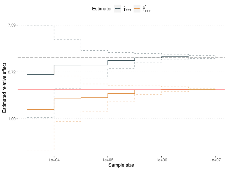
This section will illustrate the performance of the proposed estimator under different sample sizes in simulated examples. The simulations also illustrate the behaviour of the estimator in certain special cases where identifying assumptions are violated.
D.1. Data-generation
In the first scenario, the data is generated from a setting where Assumptions 1, 2, 4, and 5 hold. Let us consider individual-level data generating as follows
| (7) | |||
Let the probability of the outcome be determined by
| (8) |
where the treatment term is included in the model for the probability of the outcome in a separate logistic sigmoid function, to guarantee that the treatment has a multiplicative effect on the probability of developing the outcome.
If , then the vaccine effect is identical for both variants, hence we expect the estimate of the to be 1. In the following assume that
and .
D.2. Estiamtion of the under Assumptions 2-5
See Figure 3
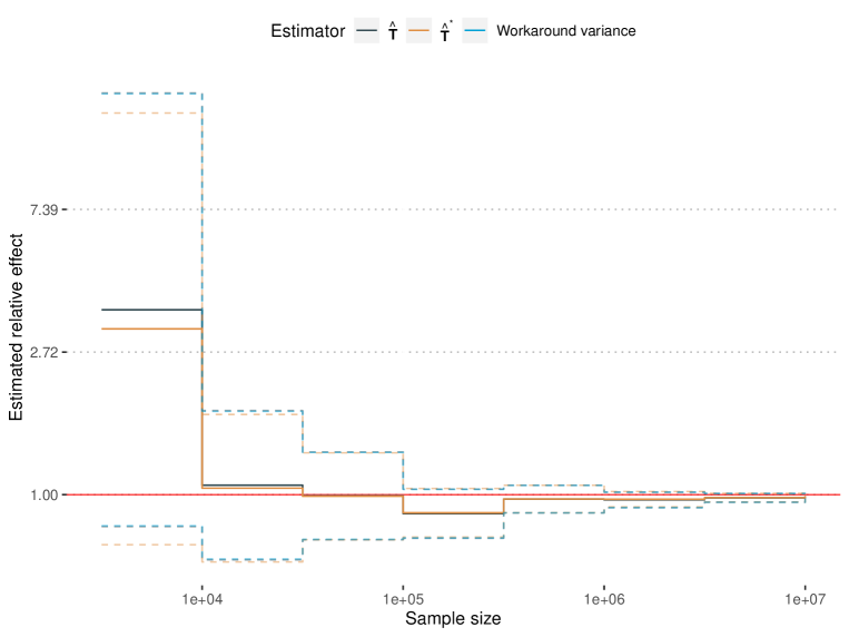
D.3. Estimation of under relaxed Assumption 2
While the data-generating process (see Equations 7) was designed to adhere to the assumption of no effect on exposure, as it was shown in Section 4, it is not a necessary condition for the identification of the , it can be relaxed to Assumption 6 instead. Thus, let us assume that
| (9) |
and leave the other elements of the data-generating mechanism unchanged.
In Figure 4, we can see that even though the estimator converges to the true contrast conditional on specific exposure, the variance increases, regardless of whether the exposure status information was used or not.
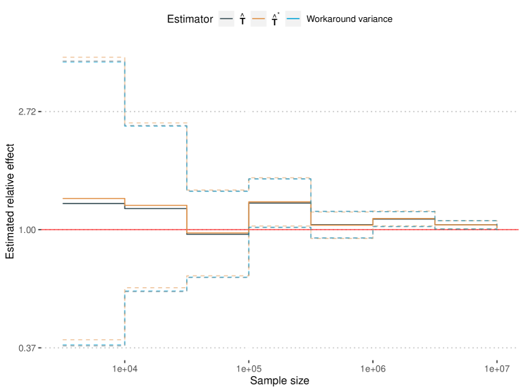
D.4. Estimation of when Assumption 6 fails
Consider the setting where neither Assumption 2 nor 6 holds. Then the formula used for the estimation of the can no longer guarantee identification. However, under the standard identifiability Assumptions 3, the estimator still identifies the ratio between the two vaccine effect estimands. Let us assume that
| (10) |
thus, the the relative exposure probabilities between the two variants, change with the treatment assignment.
In Figure 5, the estimator conditional on the exposure status converges to the true ratio between the vaccine effects for the two variants. In contrast, using the estimator based on the observed data, it converges to the ratio of the relative exposure that depends on the treatment assignments (). Thus if we were to make an assumption about this ratio, such as that it is constrained between given bounds, we could use our estimator, without conditioning on the exposure, to derive statements; such as hypothesis tests about the .
D.5. Estimation of the under Assumption S2
Consider the same data generation Equations (7) and (8). Modify the distribution of such that it satisfies Assumption S2, namely
| (11) |
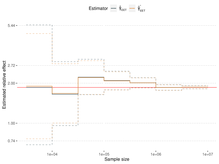
Regardless of whether we condition on the exposure status, both estimators converge to the true , with the increasing sample size, even though there are no constraints on the exposure status of the untreated, see Figure 6. Informally, since the estimators are based on the data obtained from the treated individuals, knowledge of exposures of the untreated should not change our estimates in the treated. The true is calculated based on the function for defined in Equation (8). Then the individual level is
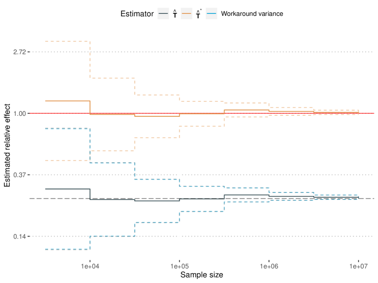
D.6. Estimation of the when Assumption S2 fails
Assume that S2 fails, and the two variants are present with different incidence rates among the population.
| (12) |
The estimator conditional on exposure status converges to the true , while it seems that the estimators based on the observed data are the systematically scaled version of that, see Figure 7. This scaling factor exactly corresponds to the unobserved ratio of exposure among the treated , that is now based on Equation 12 . If conditional exposure probabilities are unknown, then can be obtained through the assumptions discussed in Appendix E. Then after the successful estimation of this ratio, we can scale our estimator, to derive the desired ratio for the .
E. Identification assumptions and identifying functions for the and the
E.1. Effect of exposure under treatment
Assumption S1.
-
S1a
Exposure exchangeability:
-
S1b
Exposure positivity:
-
S1c
Exposure consistency:
If then and if and then .
Assumption S1a requires the measurement of common causes of the outcome and the exposure, hence imposing stronger restrictions on the data-generating mechanism, than the usual exchangeability, that is Assumption 3a. Similarly, the positivity and consistency are adjusted for the measurement of the baseline variables.
These identification assumptions are similar to the ones considered in the Appendix of Stensrud & Smith (2023) for the identification of the controlled direct effect (CDE). However, since the is the contrast of two potential outcomes in which the treatment was intervened as , Assumption S1 is defined for those variables.
Proposition 6.
See Appendix C.9 for a proof.
If the baseline covariates confounding the outcome and the are measured, then the first term in the identification formula can be straightforwardly approximated. However, estimating the second term requires the measurement of exposure, which is often not the case. Therefore to be able to identify the conditional on , if exposures remain unmeasured, further assumptions are required.
Assumption S2 (Equal exposure of the treated).
Assumption S2 is significantly stronger than Assumptions 2 and 6. While previously we only required some level of correspondence between the probabilities under the different levels of treatment assignments, Assumption S2 requires that treated individuals are exposed to both of the competing variants at the same rate. Alternatively, Assumption S2 can be experimentally assessed, by measuring the prevalence of the two competing variants, and assuming homogeneous mixing, investigators could potentially derive that the exposure probability of the treated is equal for the two variants. However, to deduce that this holds for the treated from separately collected observed data, we would need to modify our previous Assumption 6.
Assumption S3 (A conditional version of no effect on exposure ratios).
Under Assumption S3, if the observed data satisfies , then it can be concluded that Assumption S2 holds, and hence the conditional can be identified.
Lastly, data extracted from the untreated population could be used to estimate the ratio between exposure probabilities. Under the Assumptions 4 and 5, the equality holds:
Then, invoking Assumptions S1 and S3, the right-hand side is equal to
However, the ratio between and
is unknown. Thus we have to make an assumption about its value (potentially being equal to 1), to be able to estimate the conditional from the observed data.
Remark 6.
For the stronger identification assumptions to hold, Assumptions S1, values of the baseline covariates must be conditioned on. Consequently, the is expressed conditional on these baseline covariates. However, if we further assume proportionality between the potential outcomes that hold constant across the strata of , the marginal can be expressed in a simple form. We will state the assumption formally, and then provide some explanation and the identification result for the marginal .
Assumption S4.
for all .
Assumption S4 requires that under a given level of treatment and intervention on exposure, the probability of developing the outcome from variant 1, is proportional to the probability of developing the outcome from variant 2, such that the ratio between the two does not depend on the baseline covariates . Assumption S4 does not mean sieve effect or the absence of it, as it imposes no constraints on the value of . However, note that if , then the for all .
Proposition 7 (Identification of the marginal ).
The proof is provided in Appendix C.10.
E.2. Effect with intervened exposure
First, the modified identification assumptions are presented, and then the identification formula is stated.
Assumption S5.
-
S5a
Generalised exposure exchangeability:
-
S5b
Generalised exposure positivity:
-
S5c
Generalised exposure consistency:
If then and if and then .
Assumption S5a is an extension of Assumption S1a, as it requires conditional exchangeability for the untreated as well.
Similarly, the following two assumptions extend S1b and S1c for too.
Positing the stronger Assumption S5, instead of 3, and if Assumptions S3, 4, and 5 holds, we can identify the conditional effect with intervened exposure.
Proposition 8.
Remark 7.
Assumption S4 can be extended to hold for as well. Under this extension, the marginal can be identified as the fraction of conditional probabilities of the observed variables.
Assumption S6.
for all and .
Assumption S6 in itself does not imply a sieve effect either, as no constraints are applied to the relationship between and . If it is further set that , then , hence there is no (sub)population level sieve effect.
Proof is provided in Appendix C.12
E.3. Connection between and
As presented in the previous subsections, the exposure ratio of the untreated can be identified from the observed data, as long as the infectivity rate is known. Then under Assumption S3, and using Proposition 6, the conditional can be identified as
That is equal to the identification formula for the conditional under Assumptions 4, 5, S3 and S5, re-scaled by the infectivity rates of the untreated. Hence by using the notation
for the infectivity rate of the untreated, the connection between the conditional and the conditional can be summarised as
The and the can be equated under the following assumption:
Assumption S7 (Equal infectivity of the untreated).
E.4. Data example of the and the
Suppose that the identification conditions in Assumption S1 hold, conditional on the baseline variable risk profile. Thus we partition the population into High risk and Non-high risk individuals. The estimated s were ( CI: ) and ( CI: ) respectively.
However, as shown in Appendix E.1, we can replace Assumption S2, which in this setting is implausible, with Assumption S3. Then the is identified by the identification functional of the . Thus, the estimated s, and correspondingly the estimated s, for the High risk and Non-high risk are ( CI: ) and ( CI: ), respectively.
There is a qualitative difference between the two sets of estimates, in the sense that the first estimates of the show a stronger protective effect against the unmatched strain (variant 2), while the second estimates show a stronger effect against the matched strain (variant 1). Based on knowledge of vaccine mechanisms the latter is more reasonable.
Nevertheless, both estimators are designed to estimate the heterogeneity of the vaccine effect among the treated.
Here we articulate an assumption for the value of the untreated infectivity rate, to connect the and the .
Assumption S8 (Equal infectivity of the untreated).
F. Identification when individuals are lost to follow-up
Our results can be extended to a setting where individuals are possibly censored due to loss of follow-up. To ensure the identifiability of the , it must be assumed that individuals are censored independent of their counterfactual outcomes. Formally, in addition to the censoring adjusted versions of Assumptions 1, 2, 4, and 5, the following must hold.
Assumption S9 (Independent censoring).
-
S9a
-
S9b
-
S9c
Assumption S10 (Negligible multiple exposure under censoring).
Assumption S11 (No effect on exposure under censoring).
Assumption S12 (Exposure necessity under censoring).
Assumption S13 (No cross-infectivity under censoring).
Assumption S9 guarantees that the censoring event and the outcome are independent, that there is uncensored data from all levels of the treatment and the outcome, and that the observed data can be interpreted as the counterfactual outcome. Under these assumptions, the for the uncensored is identified.
Proposition 10 (Contrast conditional on specific exposure under censoring).
See Appendix C.13 for a proof.
Extension to to time-to-event settings follows analogously, see for example the appendix of Stensrud & Smith (2023).
G. Time-to-event
Following the structure introduced in Stensrud & Smith (2023), denote with and whether an individual has experienced the event by time , and being exposed to variant first, by time respectively. Hence once someone is exposed to variant , we will assume that the exposure to this given variant persists, while exposure to the competing variant is prohibited in the future. In this setting, we will define the time-to-event contrast conditional on specific exposure.
Definition 9 (Time-to-event contrast conditional on exposure).
with and .
The compares the effect of the vaccine on variant 1 and variant 2 respectively, at time among the individuals who were exposed. It is a causal estimand in the sense that the comparison is made within the same subpopulations. The following proposition ensures identification:
The proof is provided in Appendix C.14. The time-to-event is expressed as a ratio of ratios using the cumulative incidences of variant 1 and 2 respectively. Both of them can be calculated as a function of observed variables, without the measurement of common causes either between the exposure variables or the outcome variables .
H. Comments on estimation
H.1. Estimation of the
In the data example in Section 2, two regression models were fitted to estimate the hazards, for variants 1 and 2 respectively. For each of these models, outcomes corresponding to the competing variants are censoring events, as they are making the future counterfactual outcome of interest under treatment unknown (Young et al., 2020). Hence, for model 1 of variant 1, individuals who developed outcomes due to variant 2 before the end of the follow-up period, are censored at the date of the observation of this event, and correspondingly for model 2 of variant 2, individuals with observed values of are censored. Then applying the semi-parametric Cox regression, the can be expressed as the ratio of the estimated coefficients using models 1 and 2 for the two variants. The estimated coefficients are independent of time, hence the will be constant over time.
H.2. Testing Assumption 11
Assumption 11 is restrictive. However, we can construct tests to falsify this assumption even if and are not (entirely) observed: suppose that there are some observed baseline variables , such that . Then by Assumption 11, and by marginalizing over the variables , it follows that
| (13) |
By marginalizing over the same set of variables in Assumption 10 and following an argument identical to the second half of the proof of Proposition 3 (see Appendix C.4), except the modification of the conditioning set from to , Equation (13) can be rewritten to the form
The ratio of is constant across the values . Therefore, for
| (14) |
For example, by Cox regression, Equation (14) can be tested by the equality between the coefficients corresponding to in the two models of the two variants.
Assumption 11 corresponds to the null
However, is only a subset of the unobserved variables and , thus the constant proportionality assumption may hold for , but it can fail to be satisfied in a smaller sub-population defined by and , thus testing based on the subset may not be consistent.
H.3. Methods for rare events
Compared to the Cox regression model, an alternative approach for estimating the probabilities for all and are non-parametric sample means, and then we can calculate the based on this estimates. However, of the 15,955 observations, the outcome that is matched to the vaccine is developed in 86 (0.54%) cases, while the mismatched outcome is developed in 24 cases (0.15%), making them rare events. Due to the rarity of these events, the normal approximation of the estimated hazard is flawed, and consequently, the Wald-type confidence intervals of the hazards at the 6-monthly follow-ups are considerably small and invalid.
To leverage more of the observations in our estimation, the cumulative hazards were estimated instead of the hazards at times , using the conventional Nelson-Aalen (Aalen, 1978) estimator for the two models when the outcome is due to variants 1 and 2 respectively. Then the corresponding estimators are not for estimating the value of the at times , but the cumulative hazards up until the final time point. The cumulative hazard estimates were used to test a modified null hypothesis , defined as a composite between the being equal to one, and proportionality assumption on the hazards of the competing variants. Formally,
| (15) |
The proportionality assumption on the hazards is defined as an equal proportional change of the hazard ratio between the vaccine and the placebo-treated, with respect to the two strains, over time, that is
| (16) | ||||
for all . Under , the ratio of the cumulative hazards is equal to one. To increase the number of events at each time step, we combined observations from the first three visits and the observations from the last three. Then the ratios for the two periods, with Bonferroni adjusted confidence intervals are 0.23 (95% CI: 0.000, 0.613), and 0.427 (95% CI: 0.000, 0.876) respectively. Hence, under Assumptions 7-11 the null hypothesis (see Equation 15) can be rejected. However, the null requires that for all , and proportionality between the hazards, defined in Equation LABEL:EQ:_equal_vaccine_waning. Thus, even if is rejected, we cannot conclude that sieve effect is implied. Regardless, under the assumption of no sieve effect (), the ratio of the cumulative hazards must be equal to 1 in the first period, as then the ratio of cumulative hazards is equivalent to the hazard ratio. However, the same problem arises when Wald-type confidence intervals are used for rare events.
As shown in the previous paragraph, both the semi-parametric and the non-parametric approach face problems in approximation of the variance, due to the low number of uncensored events. However, when events are rare, the time-fixed and time-varying estimators will be similar. Many vaccine trials that concern infectious diseases, such as HIV, include a small proportion of events, and this implies that the vaccine effect on the competing variants can be approximated by the estimands introduced in Section 3. In the context of rare diseases, we recommend using the introduced time-fixed estimands, namely the , , and . Although Assumption 1 might be considered restrictive, the probability of multiple infectious contacts occurring over the course of the trial is negligible for diseases with low prevalence. As an illustrative example, let us denote the number of contacts that can potentially lead to infection with , for example in the case of HIV, needle sharing, or sexual contact, and let us denote with the relative prevalence of infectious individuals in the population. Then the probability of making more than infectious contact is . The relative prevalence of HIV in the US was approximately 0.36% (noa, 2023), of which a considerable amount of individuals were untransmittable, making this an over-approximation of the relative prevalence of the potentially infectious. Considering , is also an overestimation, as having more than 2 sexual partners was considered a high-risk behaviour by Rolland et al. (2012). Then the multi-exposure probability is which can be regarded as negligible, making the time-fixed estimates suitable tools for assessing the differential effect of the vaccine in the two variants.
I. Derivation of the variance and confidence intervals
If the exposure status is observed, then the can be identified from the observed data as
As the ratio of the probabilities are conditional on and respectively, they are independent. Hence the log-transformed version of this estimand can be approximated as the sum of independent normally distributed random variables. Then the ”True” variance can be derived according to Katz et al. (1978).
However, when is concealed, independence no longer holds. Regardless of this dependence between
| and |
the respective variances of the two relative risks can be derived under the log approximation and the variance of the log-transformed estimator be defined as the sum of the two. Due to the possible dependence between the two relative risks, this is an overestimation of the variance, leading to conservative confidence intervals. However, the simulation study in Appendix D shows that the loss in power endured by ignoring the correlation is negligible.
Finally, in the conditioning set could be extended , therefore the formula for is defined as
What can be noted now, is that the middle term is jointly independent of the other two, while and have a known correlation of . Thus the variance for
can be derived using Method C from Katz et al. (1978), while the variance for
follows from Katz et al. (1978) and the formula . Lastly, as these log-transformed expressions are independent, the variance can be defined as the sum of them.
The is identified using the baseline variable and data of the treated individuals only. Hence the number of cases can no longer be modeled as two independent Binomial distributions, therefore the previous method described by Katz et al. (1978) cannot be applied. Instead, we model the estimator of the as a ratio of the proportions sampled from a trinomial distribution, as by Assumption 1, . Then we can use the conservative asymptotic confidence intervals for this ratio, following the approach of Nelson (1972).
Let us denote the observed number of individuals who developed variants 1 and 2 with and respectively. Then, the two-sided confidence interval for the estimator of the is defined as
for the upper and the lower limits respectively. denotes quantile of the F-distribution with and degrees of freedom.
J. Ratio of the absolute s
Stensrud & Smith (2023) derived sharp bounds for the absolute causal effect conditional on exposure in the single variant setting. Those bounds can be equivalently used when the two competing variants are present, using Assumptions 1-5. Then the absolute ratio () is partially identified by the bounds, when
and
equivalently
The implication of these bounds is that point identification of the absolute ratio is only possible when
that can only hold, given that probabilities are bounded between and , when
Derivation of the vaccine efficacy ratio according to the definition, follows similarly, after rewriting as
Arguments for the other estimands defined in the manuscript follow analogously.