Better Gaussian Mechanism using Correlated Noise
Abstract
We present a simple variant of the Gaussian mechanism for answering differentially private queries when the sensitivity space has a certain common structure. Our motivating problem is the fundamental task of answering counting queries under the add/remove neighboring relation. The standard Gaussian mechanism solves this task by adding noise distributed as a Gaussian with variance scaled by independently to each count. We show that adding a random variable distributed as a Gaussian with variance scaled by to all counts allows us to reduce the variance of the independent Gaussian noise samples to scale only with . The total noise added to each counting query follows a Gaussian distribution with standard deviation scaled by rather than . The central idea of our mechanism is simple and the technique is flexible. We show that applying our technique to another problem gives similar improvements over the standard Gaussian mechanism.
1 Introduction
The Gaussian mechanism is one of the most important tools in differential privacy. In its most basic form, the mechanism first computes the answer to real-valued queries. The output is then perturbed by adding noise sampled from a zero-mean Gaussian distribution independently to the answer of each query. The magnitude of the Gaussian noise required to satisfy differential privacy depends on the desired privacy parameters and the sensitivity of the queries. The mechanism is used as a key subroutine in a long list of more complicated differential privacy mechanisms such as DP-SGD [ACG+16] and the Census TopDown Algorithm [AAC+22] to name just two examples (The TopDown Algorithm uses the discrete variant of the mechanism [CKS20]).
The Gaussian mechanism was introduced in some of the earliest work on differential privacy [DMNS06, DKM+06]. Since then the mechanism has been subject to a lot of study due to its importance. Notable results include a tight analysis under approximate differential privacy [BW18] as well as other definitions of differential privacy [BS16, Mir17, DRS22]. An adjacent line of work has improved the analysis of mechanisms where Gaussian noise is a key element. Recent results include an exact analysis of the Gaussian Sparse Histogram Mechanism [WKZK24] and development of numerical tools that allow for tighter privacy accounting used for DP-SGD [SMM19, KJH20, KJPH21, ZDW22]. These results give stronger privacy guarantees for various settings which leads to an improved privacy-utility trade-off. Improving the Gaussian mechanism and its variants by even small constant factors can have a significant impact on downstream applications. One notable such example is the accuracy of models trained with DP-SGD which can vary significantly based on the amount of noise (see e.g. [DBH+22, Figure 1]).
As mentioned above, the standard Gaussian mechanism privately releases queries by adding noise with magnitude scaled to the sensitivity. The sensitivity is defined as the biggest distance in the norm between the query outputs for any pair of neighboring datasets. If we have no guarantees on the norm of the query outputs we can clip data points before adding noise. This is common practice for several tasks such as approximating gradients for private machine learning (e.g. [ACG+16, KMS+21]) and mean estimation (e.g. [BDKU20, HLY21, ALNP24]). The Gaussian mechanism can be applied to many settings because we only need to bound the sensitivity to privately release an estimate to any real-value queries. However, in some cases we can achieve better error guarantees by utilizing the structure of the queries.
In this work we focus on settings where we want to estimate the sum of all data points in a dataset. We refer to the set of all possible differences between the non-private sum for neighboring dataset as the sensitivity space. We utilize a simple structure of the sensitivity space present for certain queries. Our technique reduces the magnitude of noise for such queries over the standard Gaussian mechanism that only considers the maximum norm of the sensitivity space. The structure we consider most naturally occurs under the add/remove neighboring relation. Before presenting our technique it is worth comparing the Gaussian mechanism under the add/remove and replacement neighboring relations for a query where the structure we utilize is not present. For many tasks, the sensitivity under the replacement neighboring relation is twice that of the add/remove relation. For example, if we clip the norm of data points in to some value the sensitivity is clearly under the add/remove relation. But the sensitivity is under replacement because we can replace any vector where with .
In contrast to the example above, consider the task of answering counting queries.
Here each data point is in .
The distance between neighboring datasets under add/remove is maximized when adding or removing the vector of all ones (which we denote ).
Under the replacement neighboring relation the distance is maximized by replacing any data point with one that disagrees on all coordinates.
In both cases the sensitivity is .
The standard Gaussian mechanism therefore adds noise with the same magnitude under either neighboring relation.
Our main result is to show that adding the same sample from a Gaussian distribution to all counts allows us to reduce the magnitude of the independent noise added to each query under the add/remove neighboring relation.
Theorem 10 (simplified).
Let be the answer to counting queries on dataset .
Define random variables such that , , and for any .
Then the mechanism that outputs has the same differential privacy guarantees under the add/remove neighboring relation as the mechanism that outputs .
The value of depends on the desired privacy guarantees. For simplicity of presentation we assume here that . The error of each counting query in our mechanism depends on the sum of two zero-mean Gaussian noise samples. The error is distributed as and as such the standard deviation of our mechanism is while the standard deviation for the standard Gaussian mechanism is . Note that in general we cannot hope to add Gaussian noise under add/remove for any query with less than half the magnitude required under replacement. The group privacy property of differential privacy allows us to use any mechanism designed for add/remove under the replacement relation (see e.g. [DRS22, BS16]). Our mechanism adds near-optimal Gaussian noise even for a more restrictive setting which we discuss in Section 4.1.
Many data analysis tasks depend on the size of the input dataset . However, since the size of neighboring datasets differ by under the add/remove neighboring relation we cannot release the exact size under differential privacy. This is often disregarded as a technical detail because we can estimate the size of the dataset using additional privacy budget. Some private algorithms explicitly assume that we have access to either an estimate or a bound of (see e.g. [DL09, NTZ16]). Other mechanisms implicitly rely on an estimate of the dataset size such as some versions of DP-SGD ([ACG+16]) since gradients are usually normalized based on the expected batch size which is a function of . Our mechanism also relies on an estimate of the dataset size but we do not assume that an estimate is known. We instead use part of our privacy budget to compute an estimate. There is a trade-off between the accuracy of this estimate and the error for each query which we discuss in Section 3.1. If we have access to an estimate of the dataset size we can reduce the magnitude of noise added to each query from to .
Our mechanism is simple and it is likely to be easily implementable in libraries that already support the standard Gaussian mechanism. We argue that simplicity is a desirable feature of practical differential private mechanisms. In many cases (e.g. the 2020 US Census [AAC+22]) the privately released data will be used by data analysts who might not be familiar with the theory behind differential privacy. Simple mechanisms make it easier to communicate how the data was protected and take the effect of introduced noise into account in the analysis. Furthermore, it is well known that implementations of even basic concepts and mechanisms from differential privacy requires care to avoid privacy issues (See e.g. [Mir12, CSVW22, HDH+22]). We discuss some considerations for implementation at the end of Section 3. We believe that our technique has the potential to improve mechanisms for other settings apart from counting queries. In Section 4 we adapt our core idea to a setting where we add noise with a smaller magnitude than the standard Gaussian mechanism under both the add/remove and replacement neighboring relations. We conclude our paper by discussing related work in Section 5 and potential future directions in Section 6.
2 Preliminaries
Setup of this paper. The Gaussian mechanism is used to privately estimate any real-valued function of a dataset . We focus on settings where a dataset consists of data points where and we want to estimate the sum of all data points . Throughout this paper we write to denote the set for any , we denote by the dimensional vector where all entries equal some value , and we write to denote the identity matrix.
Differential Privacy. Differential privacy [DMNS06] is a statistical property of a randomized mechanism. Intuitively, a randomized mechanism satisfies differential privacy if the output distribution of the mechanism is not affected significantly by any individual. The notion of a pair of neighboring datasets, denoted as , is used to model the impact of any one individual’s data. The two most commonly used definitions are the add/remove and replacement variants where one neighboring dataset is obtained from the other by adding, removing, or replacing any data point, respectively. We consider both definitions in this paper but focus mainly on the add/remove neighboring relation.
We present our mechanism in terms of Gaussian differential privacy (-GDP) [DRS22]. Informally, an algorithm satisfies -GDP if the output distributions for any neighboring datasets are at least as similar as two Gaussian distributions. This is more precisely defined in Definition 1.
Definition 1 (Gaussian differential privacy [DRS22, Definition 4]).
For any randomized mechanism satisfying -GDP it holds for all neighboring datasets that
Here denotes a trade-off function for two distributions and defined on the same space. The trade-off function gives a lower bound on the type 2 error achievable for any level of type 1 error. For more technical details on trade-off functions and -differential privacy we refer to Definitions 2 and 3 of [DRS22].
Note that our results do not rely on Gaussian differential privacy and can be easily translated to other popular definitions of differential privacy by replacing with an appropriate value.
Remark.
The sensitivity of a function is a restriction on the difference in output for any pair of neighboring datasets. The sensitivity of a function as defined below is a bound on the distance between the output for any pair of neighboring datasets. The sensitivity space is the set of all possible differences between outputs for neighboring datasets.
Definition 2 ( sensitivity).
The sensitivity of a function is
where denotes the norm of any .
Definition 3 (Sensitivity space).
The sensitivity space of a function is the set
The magnitude of noise added by the Gaussian mechanism scales linearly in the sensitivity and a value based on the desired privacy guarantees. Lemma 4 gives the privacy guarantees of the Gaussian mechanism. We refer to this variant as the standard Gaussian mechanism.
Lemma 4 (The Gaussian mechanism [DRS22]).
Let be a function with sensitivity . Then the mechanism that outputs where satisfies -GDP.
The last tool we need from the differential privacy literature is the fact that the privacy guarantees of a mechanism are never negatively affected by post-processing.
Lemma 5 (Post-processing [DRS22, Proposition 4]).
Let denote any mechanism satisfying -GDP. Then for any (randomized) function the composed mechanism also satisfies -GDP.
3 Algorithm
In this section we present our main contribution. The pseudo-code for our mechanism is in Algorithm 1. Throughout the section we present multiple representations of our mechanism. Each of these representations has its benefits. The error guarantees are trivial to analyze in one representation while the privacy guarantees are easier to analyze in another.
The motivating problem of our work is the differentially private release of counting queries. However, we present our mechanism in the more general setting of answering queries with a real value from the interval . That is, a dataset consists of data points such that . A pair of datasets, , are neighboring if we can obtain from by either adding or removing one data point. As such, we either have that (1) and or (2) and .
The core idea of our mechanism is to take advantage of the structure of this sensitivity space. The sensitivity of is . However, notice that the vector always has distance at most to either or (recall that denotes the dimensional vector where all coordinates are ). Our mechanism spends part of the privacy budget on adding noise along . The idea is to hide the difference between , , and . This allows us to add noise with smaller magnitude to each query. A visualization of the geometric intuition behind this idea for is shown in Figure 1.

Lemma 6.
Algorithm 1 estimates each query with error distributed as .
Proof.
It remains for us to prove the privacy guarantees of Algorithm 1. We first introduce another mechanism. We use a simple injective function to map each data point of to a point in . We then release an estimate of the sum of all data points in this new representation under -GDP using the standard Gaussian mechanism. Finally, we prove that the output distribution of Algorithm 1 is equivalent to post-processing the output of this new mechanism for a fixed parameter.
We construct from a new dataset of data points where . For each and we define and we let for some parameter . Finally, we define as the function that computes the sum of all data points in this new representation such that . The following two lemmas show that we can estimate under -GDP using the standard Gaussian mechanism.
Lemma 7.
The sensitivity of is .
Proof.
Fix any pair of neighboring datasets and let denote the data point that is either added to or removed from to obtain . It is easy to see that . By the definition of we have that is in the interval and . As such, it clearly holds that . ∎
Lemma 8.
The mechanism that outputs where satisfies -GDP.
Next, we show that Algorithm 1 and the mechanism from Lemma 8 are equivalent under post-processing when setting . Since post-processing does not affect the privacy guarantees, it follows directly from Lemma 8 and 9 that Algorithm 1 satisfies -GDP.
Lemma 9.
Proof.
By definition of the function we have that for all and . Let denote the output of . Then for we estimate the ’th value of as . Since we have that and are both distributed as . We can estimate the final entry of as . Both and are distributed as . Since the random variables of all these estimates are independent is distributed as .
Similarly, if denotes the output of we can estimate and using the inverse of . We estimate as and estimate the ’th entry of as . As such, is distributed as where is the correlated noise added to all entries. ∎
We are now ready to summarize the properties of our mechanism.
Theorem 10.
Let denote the sum of the rows in a dataset . The mechanism that outputs and where and satisfies -GDP under the add/remove neighboring relation. The error of each query is distributed as a zero-mean Gaussian with standard deviation .
Algorithm 1 relies on independent samples from Gaussian distributions. Alternatively, we can view the mechanism as outputting an estimate of and by sampling a dimensional multivariate Gaussian distribution. The entries of the covariance matrix contain one of distinct values depending on (1) whether or not it is on the diagonal and (2) whether or not it is in the final row or column. This representation might be useful for analysts for estimating the effect of noise.
Corollary 11.
Let , , and be defined as in Theorem 10 except that . Then the mechanism that outputs where satisfies -GDP under the add/remove neighboring relation where the covariance matrix has the following structure
Note for practitioners
In this section we have presented multiple representations of our mechanism. In Lemma 9 we showed that Algorithm 1 is equivalent to applying the standard Gaussian mechanism using a different representation of the dataset which we denote . However, both of these mechanisms are defined for arbitrary real-valued input and output, and as such any implementation of either representation must be an approximation of the idealized algorithm.
Real values are often approximated in computers using floating-point representation and it is well-known that naive implementations can break the formal privacy guarantees [Mir12]. Additive noise mechanisms such as the Laplace mechanism [DMNS06] and the Gaussian mechanism [DKM+06] are typically defined as releasing the sum of a non-private query output and a sample from a distribution. This can be problematic if the mechanism is implemented using floating-point arithmetics because the output domains can differ between neighboring datasets (see [HDH+22, Theorem 2]). [HDH+22] present a technique for mitigating this issue for mechanisms that add a single noisy value to the true output.
However, in line 1 of Algorithm 1 we add two noise samples to the query output which likely causes similar issues if floating-point representations are used. To the best of our knowledge, it has not been studied whether implementations of mechanisms that rely on elliptical Gaussian noise suffer from floating-point vulnerabilities. As such, implementing the version of our mechanism from Lemma 8 might be preferred for production code. The values of and can then be estimated using post-processing as described in the proof of Lemma 9. For counting queries and other discrete input we can also use the discrete Gaussian mechanism [CKS20] to estimate , although we might need to change the value of slightly when is not an integer. In Section 3.1 we discuss the effect of changing .
3.1 More accurate estimate of the dataset size
Our mechanism outputs estimates of both and the size of the dataset . So far we have ignored the accuracy of the estimate for . However, some tasks require an accurate estimate or . Here we discuss how we can release a more accurate estimate of and reduce the correlated noise by increasing the magnitude of the independent noise added to each query.
An alternative way of viewing our mechanism is that instead of estimating the value of each query independently we privately estimate the difference between and for each . We can estimate this value more accurately because has sensitivity but only has sensitivity . Given an estimate of we can then recover an estimate of . Let , denote the output of Algorithm 1. If we subtract from all outputs we find that is an estimate of the difference between and and is our estimate of . The value of itself has a sensitivity of . If we computed a new estimate for for each dimension the error would match the standard Gaussian mechanism. The advantage of our approach is that we can reuse the same private estimate of for all queries.
It is easy to see that the error for the ’th query using this representation depends on our estimates of both and . We can balance the amount of noise for each estimate which is reflected in the parameter in the representation of from earlier in this section. The magnitude of noise we use to estimate the value of is times larger than the noise for estimating .
From Lemma 8 we know that satisfies -GDP where and . Let and . Then the variance of our estimate of , , is . If we estimate as the variance of this estimate is . Notice that the dependence of for the value of is . Since the value of is minimized at which is the value we use in Lemma 9 and for Algorithm 1.
Figure 2 shows the effect of varying when . As stated above the total variance of each query is minimized for . However, the accuracy of our estimate of improves as increases. The plot shows that we can get a much more accurate estimate of while still outperforming the standard Gaussian mechanism in terms of the total variance. Even if we set such that we get an estimate of with variance only the variance for each query is which is roughly half when compared with for the standard Gaussian mechanism. The optimal choice of depends on the use case.

In this subsection we discussed the trade-off between the private estimate for the size of the input dataset and the error of each query. Throughout this paper we have assumed that we are not given an estimate of and we explicitly use part of our privacy budget to find such an estimate. However, sometimes we can assume that we have access to an estimate. This is for example the case if the mechanism is used as a subroutine in a bigger system where we already estimated the dataset size. In such cases, we are not required to spend part of our privacy budget on finding a new estimate.
Lemma 12.
Let denote the sum of the rows in a dataset . Assume that we have access to an estimate of the dataset size which we denote . Then the mechanism that outputs where satisfies -GDP under the add/remove neighboring relation.
Proof.
It follows from Lemma 4 because the sensitivity of is . ∎
4 Other settings
In the previous section we presented a simple technique for added elliptical noise for the fundamental task of privately answering queries from under the add/remove neighboring relation. This problem setting was the primary motivation for our work. However, we believe that our technique has the potential to improve the accuracy of differential private mechanisms for other settings as well. To justify this claim we consider an extension of the setting from the previous section. We improve the variance compared to the standard Gaussian mechanism for this problem under both the add/remove and the replacement neighboring relation. We end the section by comparing our technique with a recent result from related work. In Section 6 we discuss potential future extensions.
We consider a setting where a dataset consists of data points where . The input is restricted such that each data point has non-zero entries in only a single row. As such we have that . This kind of simple hierarchical data is is relevant if we are answering queries and the outputs are grouped based on some property of the data points. Two such examples would be to group users based on location or time when their data was reported. We first consider how the standard Gaussian mechanism estimates under either neighboring relation.
Lemma 13.
The mechanism that adds noise independently to each entry of distributed as satisfies -GDP under the add/remove neighboring relation. The same mechanism satisfies -GDP under the replacement neighboring relation when the noise is distributed as .
Proof.
Since the sensitivity of is clearly under the add/remove neighboring relation. Under the replacement neighboring relation and differs in at most entries by at most and as such . The privacy guarantees then follow from Lemma 4. ∎
Next, we consider how to adapt our mechanism to this setting. The main idea of Algorithm 1 is to add the same noise sample to all queries. This allows us to reduce the magnitude of the independent noise samples for each query when the sensitivity is concentrated along as shown for in Figure 1. That is not the case in this setting. Instead we sample correlated noise for each row. We also release an estimate of the number of data points with non-zero entries for each row instead of releasing an estimate of . The pseudo-code is shown in Algorithm 2.
Lemma 14.
Algorithm 2 satisfies -GDP.
Proof.
In the case of the add/remove relation and only differ in one row. Algorithm 2 essentially runs Algorithm 1 independently for each row. The privacy guarantees follow from the same proof as Lemma 9.
We prove that the privacy guarantees are correct under replacement using an alternative representation of similar to Lemma 8 for the setting of Section 3. Define such that if . By definition of the problem setup we have for all but one row for each . For the row where we define , and . We define the function .
Let denote the data point we replace with to obtains and fix the row such that . We have two cases to consider. (1) If the non-zero entries of are also in row (that is, ) then and differ by at most for each and all other entries of are unchanged. As such . (2) If the non-zero entries of are in another row the entries of and differ only in these two rows. In this case we have that .
As such, the sensitivity of under the replacement neighboring relation is and we can release under -GDP by adding noise from independently to each entry. The proof that Algorithm 2 is equivalent to post-processing the above mechanism follows the steps of the proof for Lemma 9 applied to each row for . ∎
For certain tasks we want an accurate estimate of the number of data points in each row. We can get a better estimate of the count for data points in each row () under the add/remove neighboring relation by balancing the different sources of noise similar to Section 3.1.
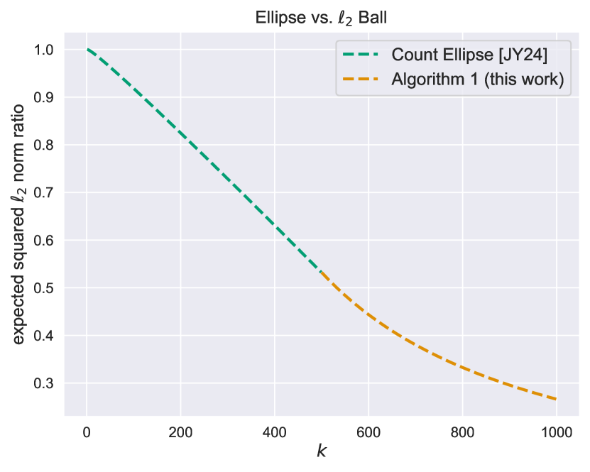
4.1 Bounded density
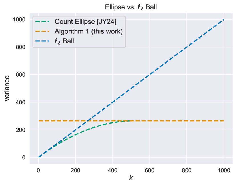
Here we consider a setting where each data point contributes to a bounded number of queries. This setting was recently studied by [JY24]. They gave efficient constructions for adding elliptical Gaussian noise for two classes of linear queries. The relevant query for this paper is the Count problem, which is equivalent to the setting from Section 3 with the additional constraint that each data point has at most non-zero entries. Similar to our mechanism they add additional noise along . They give closed-form solutions for the shape of the optimal ellipse minimizing expected squared norm. However, their result only applies when . The setting we considered in Section 3 corresponds to the case where . A natural question is whether the error can be improved for the range . It turns out that there is almost no room for improvement. In fact, our mechanism is almost optimal for any . The difference between the variance of our mechanism and the optimal ellipse of [JY24] with parameter is less than for any .
In Figure 3 we recreated a plot from Figure 1 of [JY24]. They plot the error relative to the standard Gaussian mechanism. The improvement increases with , but their mechanism is undefined for . We extended the line with our mechanism for showing the improvement for all values of . We also all three mechanisms without normalizing the variance. From the plot it is clear that their mechanism should be used for small while our mechanism is preferred for any . As a small note we point out that their mechanism does not include an estimate of the dataset size. The optimal ellipse might differ slightly if we want to return an estimate of similar to Algorithm 1.
5 Related work
The Gaussian mechanism satisfies several definitions of differential privacy. Tight bounds are known for -DP [BW18], -RDP [Mir17], -zCDP [BS16], and -GDP [DRS22]. Our privacy guarantees follow from a reduction to the standard Gaussian mechanism. As such, our results apply to any of the above definitions of differential privacy. We choose to present our mechanism in terms of -GDP because this definition exactly describes the privacy guarantees of the Gaussian mechanism. For all problems we consider in this paper our privacy guarantees for worst-case pairs of neighboring datasets exactly match those of the standard Gaussian mechanism. In technical terms, this means that there exist pairs of neighboring datasets for which the privacy loss random variable of our mechanism is distributed as . That is also the case for the standard Gaussian mechanism. We refer to [Ste22, Proposition 3] for a discussion of the privacy loss distribution of additive Gaussian noise.
[SU16] gave a lower bound on the sample complexity for answering counting queries under -differential privacy. They show that the Gaussian mechanism has asymptotical optimal error under reasonable assumptions on . The input domain in their paper is rather than . They consider the replacement neighboring relation and in that setting the counting query problem is equivalent for the two domains. It is easy to translate any estimate from one domain to the other using a simple post-processing step assuming that should be mapped . In contrast, the problem differs between the two domains under the add/remove neighboring relation. We cannot directly translate an estimate from one domain to the other using post-processing since the size of datasets is not fixed. However, the representation of the problem in the domain plays a key role in the privacy proof for our mechanism.
The mechanism we present in this paper adds unbiased correlated Gaussian noise designed to fit the structure of the queries. Adapting Gaussian noise to the shape of the sensitivity space is not a novel concept. We refer to mechanisms that add (possibly correlated) unbiased noise as general Gaussian mechanisms. [NTZ16] gave an algorithm for answering any set of linear queries under approximate differential privacy. Linear queries are a broad class of queries that includes all problems considered in this paper. They give an algorithm for choosing the shape of Gaussian noise for any linear queries by fitting an ellipse to the convex hull of the sensitivity space. [NT24] considered the problem of mean estimation under the replacement neighborhood when data points are from some bounded domain. They show that the general Gaussian mechanism achieves near-optimal error among all unbiased mechanisms for a broad class of error measures. However, their algorithm for computing the shape of noise for arbitrary queries can be inefficient.
In contrast to the general results of [NTZ16, NT24], we only consider a subset of linear queries whose sensitivity space has a certain structure. This allows us to tailor our mechanism specifically towards that structure. Concurrent with our work, [JY24] gave efficient constructions for adding elliptical Gaussian noise to two types of linear queries. They present closed-form solutions for the shape of the optimal ellipse for the Count and Vote queries. Most relevant to this paper is the Count problem which we discuss in more detail in Section 4.1. They consider the problem where entries are in rather than . Note that the problem for those settings are equivalent as we can simply scale the input by a factor of .
A recent result by [KSW24] improved the constant for private mean estimation under the add/remove neighboring relation. Their technique also includes an estimate of and an embedding of the sum in a space using an additional dimension. However, their setting differs significantly from ours and they only consider one-dimensional data making our results incomparable.
Our mechanism relies on an intermediate representation of the query outputs which can be privately estimated using the standard Gaussian mechanism. An estimate of the original queries can then be recovered using post-processing. This technique is similar to the matrix mechanism [LMH+15] used for optimizing the error of differentially private linear queries. The mechanism works by factorizing a query matrix into two new matrices. The first matrix is then applied to the input dataset and either the standard Laplace or Gaussian mechanism is used to privately release the output. The other matrix is then used to recover an estimate of the original query matrix. The technique has been used to improve mechanisms in various settings such as computing prefix sums (e.g. [HUU23, MRT22, LUZ24]).
[LT23] gave an -differentially private mechanism for releasing a Misra-Gries sketch. At a high level, their mechanism is very similar to ours. They exploit the structure of the sensitivity space of the Misra-Gries sketch and add much less noise compared to standard techniques that scale the noise by the or sensitivity. They add the same noise sample to all counters in the sketch to handle a special case where all counters differ by between some pairs of neighboring datasets. This allows them to reduce the magnitude of noise for each counter significantly because Misra-Gries sketches for neighboring datasets only differ by in a single counter except for this special case. They present some intuition behind the privacy guarantees in the technical overview of their paper using a representation similar to the one we use in Lemma 8. However, the structure of the sensitivity space for the queries we consider is different than the structure for the Misra-Gries sketch.
6 Conclusion and future work
In this paper we presented a simple variant of the general Gaussian mechanism for the fundamental task of answering independent queries in under the add/remove neighboring relation. In Section 4 we extended our mechanism to a setting where queries are divided into groups that form a partition of all queries and each data point only contributes to a single group. The general idea of our work is to take advantage of the hierarchical structure of these queries. Adding the same noise sample to all queries in a group allows us to reduce the noise added independently to each query. We believe this technique can be used to design differentially private mechanisms for other problems with similar structures. For example, we could consider settings where the groups of queries overlap instead of forming a partition. Alternatively, data points might contribute to a bounded number of groups instead of only one. In such settings we might need to increase the magnitude of correlated noise. Another interesting avenue to explore is whether correlated noise can improve constants for the Gaussian Sparse Histogram Mechanism [WKZK24]. We presented our work as a variant of the Gaussian mechanism, but a similar idea can be applied to other mechanisms such as the Laplace mechanism for pure differential privacy.
Acknowledgments
We thank Joel Daniel Andersson and other members of the Providentia project at University of Copenhagen for helpful discussions. We thank anonymous reviewers for suggestions that helped improve the paper.
References
- [AAC+22] John M. Abowd, Robert Ashmead, Ryan Cumings-Menon, Simson L. Garfinkel, Micah Heineck, Christine Heiss, Robert Johns, Daniel Kifer, Philip Leclerc, Ashwin Machanavajjhala, Brett Moran, William Sexton, Matthew Spence, and Pavel Zhuravlev. The 2020 census disclosure avoidance system topdown algorithm. Harvard Data Science Review, 2, 2022.
- [ACG+16] Martín Abadi, Andy Chu, Ian J. Goodfellow, H. Brendan McMahan, Ilya Mironov, Kunal Talwar, and Li Zhang. Deep learning with differential privacy. In CCS, pages 308–318. ACM, 2016.
- [ALNP24] Martin Aumüller, Christian Janos Lebeda, Boel Nelson, and Rasmus Pagh. PLAN: variance-aware private mean estimation. Proc. Priv. Enhancing Technol., 2024(3):606–625, 2024.
- [BDKU20] Sourav Biswas, Yihe Dong, Gautam Kamath, and Jonathan Ullman. CoinPress: Practical Private Mean and Covariance Estimation. Advances in Neural Information Processing Systems, 33:14475–14485, 2020.
- [BS16] Mark Bun and Thomas Steinke. Concentrated differential privacy: Simplifications, extensions, and lower bounds. In Theory of Cryptography Conference, pages 635–658. Springer, 2016.
- [BW18] Borja Balle and Yu-Xiang Wang. Improving the gaussian mechanism for differential privacy: Analytical calibration and optimal denoising. In ICML, volume 80 of Proceedings of Machine Learning Research, pages 403–412. PMLR, 2018.
- [CKS20] Clément L. Canonne, Gautam Kamath, and Thomas Steinke. The discrete gaussian for differential privacy. In Advances in Neural Information Processing Systems 33: Annual Conference on Neural Information Processing Systems 2020, NeurIPS 2020, December 6-12, 2020, virtual, 2020.
- [CSVW22] Sílvia Casacuberta, Michael Shoemate, Salil P. Vadhan, and Connor Wagaman. Widespread underestimation of sensitivity in differentially private libraries and how to fix it. In Proceedings of the 2022 ACM SIGSAC Conference on Computer and Communications Security, CCS 2022, Los Angeles, CA, USA, November 7-11, 2022, pages 471–484. ACM, 2022.
- [DBH+22] Soham De, Leonard Berrada, Jamie Hayes, Samuel L Smith, and Borja Balle. Unlocking high-accuracy differentially private image classification through scale. arXiv preprint arXiv:2204.13650, 2022.
- [DKM+06] Cynthia Dwork, Krishnaram Kenthapadi, Frank McSherry, Ilya Mironov, and Moni Naor. Our data, ourselves: Privacy via distributed noise generation. In Advances in Cryptology - EUROCRYPT 2006, 25th Annual International Conference on the Theory and Applications of Cryptographic Techniques, St. Petersburg, Russia, May 28 - June 1, 2006, Proceedings, volume 4004 of Lecture Notes in Computer Science, pages 486–503. Springer, 2006.
- [DL09] Cynthia Dwork and Jing Lei. Differential privacy and robust statistics. In Proceedings of the 41st Annual ACM Symposium on Theory of Computing, STOC 2009, Bethesda, MD, USA, May 31 - June 2, 2009, pages 371–380. ACM, 2009.
- [DMNS06] Cynthia Dwork, Frank McSherry, Kobbi Nissim, and Adam D. Smith. Calibrating noise to sensitivity in private data analysis. In Theory of Cryptography, Third Theory of Cryptography Conference, TCC 2006, New York, NY, USA, March 4-7, 2006, Proceedings, volume 3876 of Lecture Notes in Computer Science, pages 265–284. Springer, 2006.
- [DRS22] Jinshuo Dong, Aaron Roth, and Weijie J Su. Gaussian differential privacy. Journal of the Royal Statistical Society: Series B (Statistical Methodology), 84(1):3–37, 2022.
- [HDH+22] Samuel Haney, Damien Desfontaines, Luke Hartman, Ruchit Shrestha, and Michael Hay. Precision-based attacks and interval refining: how to break, then fix, differential privacy on finite computers. CoRR, abs/2207.13793, 2022.
- [HLY21] Ziyue Huang, Yuting Liang, and Ke Yi. Instance-optimal Mean Estimation Under Differential Privacy. Advances in Neural Information Processing Systems, 34:25993–26004, 2021.
- [HUU23] Monika Henzinger, Jalaj Upadhyay, and Sarvagya Upadhyay. Almost tight error bounds on differentially private continual counting. In Proceedings of the 2023 ACM-SIAM Symposium on Discrete Algorithms, SODA 2023, Florence, Italy, January 22-25, 2023, pages 5003–5039. SIAM, 2023.
- [JY24] Matthew Joseph and Alexander Yu. Some constructions of private, efficient, and optimal k-norm and elliptic gaussian noise. In The Thirty Seventh Annual Conference on Learning Theory, June 30 - July 3, 2023, Edmonton, Canada, volume 247 of Proceedings of Machine Learning Research, pages 2723–2766. PMLR, 2024.
- [KJH20] Antti Koskela, Joonas Jälkö, and Antti Honkela. Computing tight differential privacy guarantees using fft. In Proceedings of the Twenty Third International Conference on Artificial Intelligence and Statistics, volume 108 of Proceedings of Machine Learning Research, pages 2560–2569. PMLR, 26–28 Aug 2020.
- [KJPH21] Antti Koskela, Joonas Jälkö, Lukas Prediger, and Antti Honkela. Tight differential privacy for discrete-valued mechanisms and for the subsampled gaussian mechanism using FFT. In AISTATS, volume 130 of Proceedings of Machine Learning Research, pages 3358–3366. PMLR, 2021.
- [KMS+21] Peter Kairouz, Brendan McMahan, Shuang Song, Om Thakkar, Abhradeep Thakurta, and Zheng Xu. Practical and private (deep) learning without sampling or shuffling. In Proceedings of the 38th International Conference on Machine Learning, ICML 2021, 18-24 July 2021, Virtual Event, volume 139 of Proceedings of Machine Learning Research, pages 5213–5225. PMLR, 2021.
- [KSW24] Alex Kulesza, Ananda Theertha Suresh, and Yuyan Wang. Mean estimation in the add-remove model of differential privacy. In Forty-first International Conference on Machine Learning, 2024.
- [LMH+15] Chao Li, Gerome Miklau, Michael Hay, Andrew McGregor, and Vibhor Rastogi. The matrix mechanism: optimizing linear counting queries under differential privacy. VLDB J., 24(6):757–781, 2015.
- [LT23] Christian Janos Lebeda and Jakub Tetek. Better differentially private approximate histograms and heavy hitters using the misra-gries sketch. In Proceedings of the 42nd ACM SIGMOD-SIGACT-SIGAI Symposium on Principles of Database Systems, PODS 2023, Seattle, WA, USA, June 18-23, 2023, pages 79–88. ACM, 2023.
- [LUZ24] Jingcheng Liu, Jalaj Upadhyay, and Zongrui Zou. Optimality of matrix mechanism on -metric. CoRR, abs/2406.02140, 2024.
- [Mir12] Ilya Mironov. On significance of the least significant bits for differential privacy. In Proceedings of the 2012 ACM Conference on Computer and Communications Security, CCS ’12, page 650–661, New York, NY, USA, 2012. Association for Computing Machinery.
- [Mir17] Ilya Mironov. Rényi differential privacy. In 2017 IEEE 30th computer security foundations symposium (CSF), pages 263–275. IEEE, 2017.
- [MRT22] Brendan McMahan, Keith Rush, and Abhradeep Guha Thakurta. Private online prefix sums via optimal matrix factorizations. CoRR, abs/2202.08312, 2022.
- [NT24] Aleksandar Nikolov and Haohua Tang. General gaussian noise mechanisms and their optimality for unbiased mean estimation. In 15th Innovations in Theoretical Computer Science Conference, ITCS 2024, January 30 to February 2, 2024, Berkeley, CA, USA, volume 287 of LIPIcs, pages 85:1–85:23. Schloss Dagstuhl - Leibniz-Zentrum für Informatik, 2024.
- [NTZ16] Aleksandar Nikolov, Kunal Talwar, and Li Zhang. The geometry of differential privacy: The small database and approximate cases. SIAM Journal on Computing, 45(2):575–616, 2016.
- [SMM19] David M. Sommer, Sebastian Meiser, and Esfandiar Mohammadi. Privacy loss classes: The central limit theorem in differential privacy. Proc. Priv. Enhancing Technol., 2019(2):245–269, 2019.
- [Ste22] Thomas Steinke. Composition of differential privacy & privacy amplification by subsampling. arXiv preprint arXiv:2210.00597, 2022.
- [SU16] Thomas Steinke and Jonathan R. Ullman. Between pure and approximate differential privacy. J. Priv. Confidentiality, 7(2), 2016.
- [WKZK24] Arjun Wilkins, Daniel Kifer, Danfeng Zhang, and Brian Karrer. Exact privacy analysis of the gaussian sparse histogram mechanism. Journal of Privacy and Confidentiality, 14(1), Feb. 2024.
- [ZDW22] Yuqing Zhu, Jinshuo Dong, and Yu-Xiang Wang. Optimal accounting of differential privacy via characteristic function. In Proceedings of The 25th International Conference on Artificial Intelligence and Statistics, volume 151 of Proceedings of Machine Learning Research, pages 4782–4817. PMLR, 28–30 Mar 2022.