Analytic solutions for the motion of spinning particles near brane-world black hole

Yunlong Liu Department of Physics, South China University of Technology, Guangzhou 510641, China โ€ƒโ€ƒ Xiangdong Zhang111Corresponding author. scxdzhang@scut.edu.cn Department of Physics, South China University of Technology, Guangzhou 510641, China
Abstract

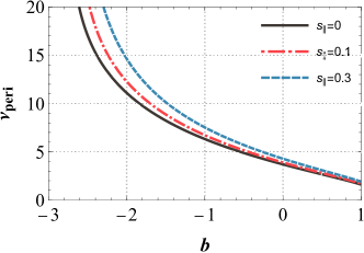
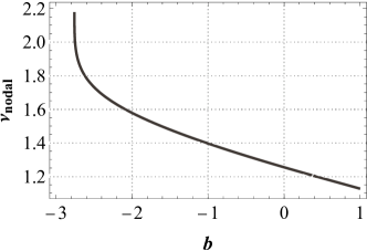
The general motion of spinning test particles to the leading order approximation of spin in the brane-world spacetime is investigated. Analytical integrations for the equations of motion and linear shifts in orbital frequency are obtained. As a result, we found that both the nodal precession and the periastron precession become larger when the tidal charge $b$ of brane-world spacetime becomes smaller. For the periastron precession, the effect is further amplified as the spin increases. Our work can potentially be applied to the study of gravitational waveforms of Extreme Mass Ratio Inspirals with spin in brane-world spacetime.

I Introduction

It has been nearly 10 years since LIGO first directly detected gravitational waves(GWs) [1], ground-based GW detection technology has been continuously updated and iterated, and the number of observed events has steadily increased [2, 3, 4]. More notably, space-based GW detectors such as LISA [5], Taiji [7, 6], and TianQin [8] are also being developed intensively. These detectors can extend the sensitivity range to lower frequencies. It means that they could observe a special class of binary systems known as Extreme Mass Ratio Inspirals (EMRIs) [9] that describe a system where a small secondary object orbits a supermassive primary one. Analyzing the GW signals from EMRIs allows us to explore the nature of compact objects at the center of galaxies as well as to test the General relativity(GR) [10].

Modeling the gravitational waveforms of EMRIs typically involves expansion in the mass ratio. In the leading order, adiabatic methods for EMRIs encodes the spiral inward of the secondary object that caused by GW fluxes along with the geodesic [11, 12], while the first post-adiabatic order includes conservative self-force effects and the spin of the test body [13]. These post-adiabatic effects, particularly the spin of the test particle, have a crucial impact on the data analysis and modeling of gravitational waveforms [14, 15]. To further explore the dynamics of EMRI systems with spins, there are primarily two approaches: the post-Newtonian(PN) approximation schemes [16, 17, 18, 19, 20, 21, 22] and effective-one-body(EOB) schemes [23, 24, 25]. At the same time, many papers have studied the effects of spin on physics such as the innermost stable orbits(ISO) [26], collisional Penrose processes [27], black hole accretors [28], gravitational waveforms [29]. However, since test bodyโ€™s spin couples to the curvature of that spacetime, we need to consider the spin-curvature force and must be modeled carefully in order to accurately characterize the motion of bodies orbiting black holes. In order to have a better understanding on these important issues. Recently, an analytic solution for the motion of spinning particles to leading order in spin in the static and spherically symmetric spacetimes has been provided in [30] along [31, 33, 32]. As a result, they obtain the bound orbits in Schwarzschild space-time by expressing the solution in the form of Jacobi elliptic functions.

On the other hand, to unify gravity with other fundamental forces, an elegant scheme is the extra dimensions theory, such as the Kaluza-Klein (KK) model[34, 35] and the later the string/M-theory, both hypothesize the existence of extra dimensions at the Planck scale, which are currently difficult to detect with experiments. Differently, as an effective four-dimensional version of high-dimensional string theory, the brane-world model[36, 37] posits that our physical universe is embedded in a higher-dimensional spacetime (bulk), with standard model matter and fields trapped on the brane. Interestingly, a black hole solution can be obtained in the brane-world model [38], characterized by the tidal charge $b$. This in turn provides a framework to study the physical effects caused by extra dimensions [41, 42, 40, 39].

Given the above motivation and considering the importance of analytic solutions. In this paper, we aimed to generalize the analytic solutions obtained in [30] to brane-world spacetime and discusses the physical consequence of the tilde charge parameter $b$.

The structure of this article is as follows: In Sec. II, the background spacetime is introduced and the corresponding equations of motion are provided. Sec. III introduces parallel transport of spin and provides the evolution of spin components. In Sec. III, the Kepler-parameter expressions of energy, angular momentum, and the roots of radial velocity are given. Sec. V and VI respectively presented analytic results of motion and linear shifts in orbital frequencies. Finally, in sec. VII, some conclusions and corresponding discussions are provided. Through out the paper, the geometrized units with $G=c=1$ and the metric signature ($-+++$) are used.

II Equations of motion

II.1 Brane-world background

The field equations on the bulk(5 dimensions) and the reduced equations of motions on brane(4 dimensions) is given respectively as [36]

$\displaystyle G^{(5)}_{AB}$ $\displaystyle=$ $\displaystyle-\tilde{\Lambda}g^{(5)}_{AB}+\tilde{\kappa}^{2}T^{(5)}_{AB},$ (1)
$\displaystyle G_{\mu\nu}$ $\displaystyle=$ $\displaystyle-\Lambda g_{\mu\nu}+\kappa^{2}T_{\mu\nu}+\tilde{\kappa}^{4}\mathcal{S}_{\mu\nu}-\mathcal{T}_{\mu\nu},$ (2)

where $\tilde{\Lambda}$ is the 5-dimensional negative cosmological constant, $T^{(5)}_{AB}$ represents 5-dimensional energy-momentum, and $\tilde{\kappa}^{2}=8\pi/\tilde{M}_{p}^{3}$ with $\tilde{M}_{p}$ being 5-dimensional Planck mass in the bulk. Meanwhile, $\kappa^{2}=8\pi/M_{p}^{2}=\lambda\tilde{\kappa}^{4}/6$ and $\Lambda=\tilde{\kappa}^{2}(\tilde{\Lambda}+\tilde{\kappa}^{2}\lambda^{2})/2$ where $\Lambda$, $M_{p}$ and $\lambda$ represent the cosmological constants, effective Planck mass and brane tension in the brane, respectively. Here, we just consider the case where $\tilde{\Lambda}=-\tilde{\kappa}^{2}\lambda^{2}$. $T_{\mu\nu}$ and $\mathcal{S}_{\mu\nu}$ are the energy momentum and its quadratic parts, separately. Moreover, $\mathcal{T}_{\mu\nu}$ is the projected Weyl tensor on the brane [36].

We usually assume that there is no exchange of energy-momentum between the bulk and brane in order to obtain conservation equations [37] as

$\displaystyle\nabla^{\nu}T_{\mu\nu}=-2T^{(5)}_{AB}n^{A}g^{B}_{\mu}=0,$ (3)

where $\nabla_{\nu}$ is the covariant derivative on the brane. This means that, we can naturally use the โ€œdynamical equationโ€ of spin particles with only changing the background metric in the brane-world.

On the other hand, we have

$\displaystyle\nabla^{\nu}\mathcal{T}_{\mu\nu}=\tilde{\kappa}^{4}\nabla^{\nu}\mathcal{S}_{\mu\nu}.$ (4)

For test bodies, in the low-energy approximation [36, 37], we assume that the quadratic energy-momentum tensor $\mathcal{S}_{\mu\nu}$ has a negligible impact on the background spacetime. It leads to $\nabla^{\nu}\mathcal{T}_{\mu\nu}\approx 0$. Hence, We can apply the conclusion of [38] and obtain the metric of the brane-world [38]:

dโ€‹s2=โˆ’fโ€‹[r]โ€‹dโ€‹t2+1fโ€‹[r]โ€‹dโ€‹r2+r2โ€‹(dโ€‹ฮธ2+sin2โกฮธโ€‹dโ€‹ฯ•2),๐‘‘superscript๐‘ 2๐‘“delimited-[]๐‘Ÿ๐‘‘superscript๐‘ก21๐‘“delimited-[]๐‘Ÿ๐‘‘superscript๐‘Ÿ2superscript๐‘Ÿ2๐‘‘superscript๐œƒ2superscript2๐œƒ๐‘‘superscriptitalic-ฯ•2\displaystyle ds^{2}=-f[r]dt^{2}+\frac{1}{f[r]}dr^{2}+r^{2}\left(d\theta^{2}+\sin^{2}\theta d\phi^{2}\right), (5)

where,$f[r]=1-2M/r+M^{2}b/r^{2}$. Here, $M$ is the mass of the black hole, and $b$ is the tidal charge parameter arising from the bulk Weyl field. When $f[r]=0$ , corresponding to two horizons of the black hole:

$$r_{n}=M\left(1-\sqrt{1-b}\right),\quad r_{p}=M\left(1+\sqrt{1-b}\right),$$ (6)

where, the range of $b$ is constrained as $b\leq 1$.

II.2 Leading order in small spin

In curved spacetime, any distribution of mass or other properties will cause the particle to move away from the geodesic. For a spinning test body, in brane world spacetime, the motion can be described by the famous Mathissionโ€“Papapetrouโ€“Dixon (MPD) equations as [43, 44, 45]:

$\displaystyle\frac{DP^{\mu}}{d\tau}$ $\displaystyle=$ $\displaystyle-\frac{1}{2}R^{\mu}{}_{\nu\alpha\beta}\dot{x}^{\nu}S^{\alpha\beta},$ (7)
$\displaystyle\frac{DS^{\mu\nu}}{d\tau}$ $\displaystyle=$ $\displaystyle P^{\mu}\dot{x}^{\nu}-P^{\nu}\dot{x}^{\mu},$ (8)

where $\dot{x}^{\mu}=dx^{\mu}/dt$, $P^{\mu}$ and $S^{\mu\nu}$ respectively represent tangent vector to the worldline of test particle, 4-momentum and the spin angular momentum tensor.

The MPD equations is not sufficient for the evolution of all degrees of freedom. Hence, spin supplementary condition (SSC) should be required. We commonly adopt the form proposed by Tulczyjew-Dixon (TD) [46, 44], given by $S^{\mu\nu}P_{\nu}=0$. With this condition, the four-velocity $\dot{x}^{\mu}$ and the four-momentum $P^{\mu}$ are not parallel. However, if we consider only the linear order of spin, we can obtain:

$\displaystyle-P_{\mu}\dot{x}^{\mu}$ $\displaystyle=$ $\displaystyle m+\mathcal{O}[S^{2}],$ (9)
$\displaystyle P^{\mu}$ $\displaystyle=$ $\displaystyle m\dot{x}^{\mu}+\mathcal{O}[S^{2}].$ (10)

Here, $m$ represents the mass of the spinning test body. Similarly, the spin tensor is antisymmetric, and approximately expressed as:

Sฮฑโ€‹ฮฒ=mโ€‹ฯตฮฑโ€‹ฮฒโ€‹ฮผโ€‹ฮฝโ€‹xห™ฮผโ€‹sฮฝ+๐’ชโ€‹[S2],superscript๐‘†๐›ผ๐›ฝ๐‘šsuperscriptitalic-ฯต๐›ผ๐›ฝ๐œ‡๐œˆsubscriptห™๐‘ฅ๐œ‡subscript๐‘ ๐œˆ๐’ชdelimited-[]superscript๐‘†2\displaystyle S^{\alpha\beta}=m\epsilon^{\alpha\beta\mu\nu}\dot{x}_{\mu}s_{\nu}+\mathcal{O}[S^{2}], (11)

where sฮฝsuperscript๐‘ ๐œˆs^{\nu} is the specific spin vector. Meanwhile, the TD condition transforms into sฮฝโ€‹xห™ฮฝ=0superscript๐‘ ๐œˆsubscriptห™๐‘ฅ๐œˆ0s^{\nu}\dot{x}_{\nu}=0. This implies that sฮฝsuperscript๐‘ ๐œˆs^{\nu} is a spatial vector.

Finally, the MPD equations of motion can be reformulated as:

$\displaystyle\frac{D^{2}x^{\mu}}{d\tau^{2}}$ $\displaystyle=$ โˆ’12โ€‹Rฮผโ€‹ฯตฮฑโ€‹ฮฒฮฝโ€‹ฮฑโ€‹ฮฒโ€‹xห™ฮฝฮปโ€‹ฯƒโ€‹xห™ฮปโ€‹sฯƒ,12superscript๐‘…๐œ‡subscriptsuperscriptitalic-ฯต๐›ผ๐›ฝ๐œˆ๐›ผ๐›ฝsubscriptsuperscriptห™๐‘ฅ๐œˆ๐œ†๐œŽsuperscriptห™๐‘ฅ๐œ†superscript๐‘ ๐œŽ\displaystyle-\frac{1}{2}R^{\mu}{}_{\nu\alpha\beta}\epsilon^{\alpha\beta}{}_{\lambda\sigma}\dot{x}^{\nu}\dot{x}^{\lambda}s^{\sigma}, (12)
Dโ€‹sฮผdโ€‹ฯ„๐ทsuperscript๐‘ ๐œ‡๐‘‘๐œ\displaystyle\frac{Ds^{\mu}}{d\tau} $\displaystyle=$ $\displaystyle 0.$ (13)

It can be seen that at the linear order, the spin vector undergoes parallel transport along the world line.

II.3 Equations of motion

In spherically symmetric spacetime, there exist Killing vector fields

$\displaystyle\xi_{(t)\mu}$ $\displaystyle=$ $\displaystyle\{1,0,0,0\},$ (14)
$\displaystyle\xi_{(x)\mu}$ $\displaystyle=$ $\displaystyle\{0,0,-\sin\phi,-\cos\phi\cot\theta\},$ (15)
$\displaystyle\xi_{(y)\mu}$ $\displaystyle=$ $\displaystyle\{0,0,\cos\phi,-\sin\phi\cot\theta\},$ (16)
$\displaystyle\xi_{(z)\mu}$ $\displaystyle=$ $\displaystyle\{0,0,0,1\}.$ (17)

These Killing vector fields correspond to time translations and spatial rotations, respectively.

Correspondingly, the conserved quantity for motion with the given Killing vector field in the brane-world spacetime reads

$\displaystyle C_{(\xi)}=P^{\mu}\xi_{\mu}-\xi_{\rho;\sigma}S^{\rho\sigma}/2.$ (18)

Using the Killing vector fields, the energy and angular momentum of a test particle can be described as:

$\displaystyle\mathcal{E}$ $\displaystyle=$ fโ€‹tห™+12โ€‹r2โ€‹sinโกฮธโ€‹(sฯ•โ€‹ฮธห™โˆ’sฮธโ€‹ฯ•ห™)โ€‹fโ€ฒโ€‹[r],๐‘“ห™๐‘ก12superscript๐‘Ÿ2๐œƒsuperscript๐‘ italic-ฯ•ห™๐œƒsuperscript๐‘ ๐œƒห™italic-ฯ•superscript๐‘“โ€ฒdelimited-[]๐‘Ÿ\displaystyle f\dot{t}+\frac{1}{2}r^{2}\sin\theta\left(s^{\phi}\dot{\theta}-s^{\theta}\dot{\phi}\right)f^{\prime}[r], (19)
$\displaystyle\mathcal{J}_{x}$ $\displaystyle=$ r2โ€‹(โˆ’ฯ•ห™โ€‹cosโกฮธโ€‹cosโกฯ•โ€‹sinโกฮธโˆ’ฮธห™โ€‹sinโกฯ•)+cosโกฯ•โ€‹sinโกฮธโ€‹(rห™โ€‹stโˆ’tห™โ€‹sr)superscript๐‘Ÿ2ห™italic-ฯ•๐œƒitalic-ฯ•๐œƒห™๐œƒitalic-ฯ•italic-ฯ•๐œƒห™๐‘Ÿsuperscript๐‘ ๐‘กห™๐‘กsuperscript๐‘ ๐‘Ÿ\displaystyle r^{2}\left(-\dot{\phi}\cos\theta\cos\phi\sin\theta-\dot{\theta}\sin\phi\right)+\cos\phi\sin\theta\left(\dot{r}s^{t}-\dot{t}s^{r}\right) (20)
+rโ€‹fโ€‹[r]โ€‹(cosโกฮธโ€‹cosโกฯ•โ€‹(ฮธห™โ€‹stโ€‹โˆ’โ€‹tห™โ€‹sฮธ)+sinโกฮธโ€‹sinโกฯ•โ€‹(โˆ’โ€‹ฯ•ห™โ€‹st+tห™โ€‹sฯ•)),๐‘Ÿ๐‘“delimited-[]๐‘Ÿ๐œƒitalic-ฯ•ห™๐œƒsuperscript๐‘ ๐‘กโˆ’ห™๐‘กsuperscript๐‘ ๐œƒ๐œƒitalic-ฯ•โˆ’ห™italic-ฯ•superscript๐‘ ๐‘กห™๐‘กsuperscript๐‘ italic-ฯ•\displaystyle+rf[r]\left(\cos\theta\cos\phi\left(\dot{\theta}s^{t}โˆ’\dot{t}s^{\theta}\right)+\sin\theta\sin\phi\left(โˆ’\dot{\phi}s^{t}+\dot{t}s^{\phi}\right)\right),
$\displaystyle\mathcal{J}_{y}$ $\displaystyle=$ r2โ€‹(ฮธห™โ€‹cosโกฯ•โˆ’ฯ•ห™โ€‹cosโกฮธโ€‹sinโกฮธโ€‹sinโกฯ•)+sinโกฮธโ€‹sinโกฯ•โ€‹(rห™โ€‹stโˆ’tห™โ€‹sr)superscript๐‘Ÿ2ห™๐œƒitalic-ฯ•ห™italic-ฯ•๐œƒ๐œƒitalic-ฯ•๐œƒitalic-ฯ•ห™๐‘Ÿsuperscript๐‘ ๐‘กห™๐‘กsuperscript๐‘ ๐‘Ÿ\displaystyle r^{2}\left(\dot{\theta}\cos\phi-\dot{\phi}\cos\theta\sin\theta\sin\phi\right)+\sin\theta\sin\phi\left(\dot{r}s^{t}-\dot{t}s^{r}\right) (21)
+rโ€‹fโ€‹[r]โ€‹(cosโกฮธโ€‹sinโกฯ•โ€‹(ฮธห™โ€‹stโˆ’tห™โ€‹sฮธ)+cosโกฯ•โ€‹sinโกฮธโ€‹(ฯ•ห™โ€‹stโˆ’tห™โ€‹sฯ•)),๐‘Ÿ๐‘“delimited-[]๐‘Ÿ๐œƒitalic-ฯ•ห™๐œƒsuperscript๐‘ ๐‘กห™๐‘กsuperscript๐‘ ๐œƒitalic-ฯ•๐œƒห™italic-ฯ•superscript๐‘ ๐‘กห™๐‘กsuperscript๐‘ italic-ฯ•\displaystyle+rf[r]\left(\cos\theta\sin\phi\left(\dot{\theta}s^{t}-\dot{t}s^{\theta}\right)+\cos\phi\sin\theta\left(\dot{\phi}s^{t}-\dot{t}s^{\phi}\right)\right),
$\displaystyle\mathcal{J}_{z}$ $\displaystyle=$ r2โ€‹sin2โกฮธ+cosโกฮธโ€‹(rห™โ€‹stโˆ’tห™โ€‹s1)+rโ€‹fโ€‹[r]โ€‹sinโกฮธโ€‹(โˆ’ฮธห™โ€‹st+tห™โ€‹sฮธ).superscript๐‘Ÿ2superscript2๐œƒ๐œƒห™๐‘Ÿsuperscript๐‘ ๐‘กห™๐‘กsuperscript๐‘ 1๐‘Ÿ๐‘“delimited-[]๐‘Ÿ๐œƒห™๐œƒsuperscript๐‘ ๐‘กห™๐‘กsuperscript๐‘ ๐œƒ\displaystyle r^{2}\sin^{2}\theta+\cos\theta\left(\dot{r}s^{t}-\dot{t}s^{1}\right)+rf[r]\sin\theta\left(-\dot{\theta}s^{t}+\dot{t}s^{\theta}\right). (22)

Here, $\mathcal{E}$, $\mathcal{J}_{x}$, $\mathcal{J}_{y}$, and $\mathcal{J}_{z}$ are all normalized by the test particleโ€™s mass $m$. We can always reselect the aligned coordinate system such that the angular momenta $\mathcal{J}_{x}=0$, $\mathcal{J}_{y}=0$, and $\mathcal{J}_{z}=\mathcal{J}$. Then, we assume the $\theta$ satisfies $\theta=\pi/2+\delta\theta$. Substituting into Eqs. (20)-(21) and expanding in terms of $\delta\theta$, we obtain

$\displaystyle\mathcal{J}_{x}$ $\displaystyle=$ โˆ’sinโกฯ•โ€‹(ฮดโ€‹ฮธห™โ€‹r2+rโ€‹fโ€‹[r]โ€‹(ฯ•ห™โ€‹stโˆ’tห™โ€‹sฯ•))+cosโกฯ•โ€‹(rห™โ€‹stโˆ’tห™โ€‹sr+ฯ•ห™โ€‹r2โ€‹ฮดโ€‹ฮธ),italic-ฯ•ห™๐›ฟ๐œƒsuperscript๐‘Ÿ2๐‘Ÿ๐‘“delimited-[]๐‘Ÿห™italic-ฯ•superscript๐‘ ๐‘กห™๐‘กsuperscript๐‘ italic-ฯ•italic-ฯ•ห™๐‘Ÿsuperscript๐‘ ๐‘กห™๐‘กsuperscript๐‘ ๐‘Ÿห™italic-ฯ•superscript๐‘Ÿ2๐›ฟ๐œƒ\displaystyle-\sin\phi\left(\dot{\delta\theta}r^{2}+rf[r]\left(\dot{\phi}s^{t}-\dot{t}s^{\phi}\right)\right)+\cos\phi\left(\dot{r}s^{t}-\dot{t}s^{r}+\dot{\phi}r^{2}\delta\theta\right), (23)
$\displaystyle\mathcal{J}_{y}$ $\displaystyle=$ cosโกฯ•โ€‹(ฮดโ€‹ฮธห™โ€‹r2+rโ€‹fโ€‹[r]โ€‹(ฯ•ห™โ€‹stโˆ’tห™โ€‹sฯ•))+sinโกฯ•โ€‹(rห™โ€‹stโˆ’tห™โ€‹sr+ฯ•ห™โ€‹r2โ€‹ฮดโ€‹ฮธ).italic-ฯ•ห™๐›ฟ๐œƒsuperscript๐‘Ÿ2๐‘Ÿ๐‘“delimited-[]๐‘Ÿห™italic-ฯ•superscript๐‘ ๐‘กห™๐‘กsuperscript๐‘ italic-ฯ•italic-ฯ•ห™๐‘Ÿsuperscript๐‘ ๐‘กห™๐‘กsuperscript๐‘ ๐‘Ÿห™italic-ฯ•superscript๐‘Ÿ2๐›ฟ๐œƒ\displaystyle\cos\phi\left(\dot{\delta\theta}r^{2}+rf[r]\left(\dot{\phi}s^{t}-\dot{t}s^{\phi}\right)\right)+\sin\phi\left(\dot{r}s^{t}-\dot{t}s^{r}+\dot{\phi}r^{2}\delta\theta\right). (24)

To make $\mathcal{J}_{x}=0$ and $\mathcal{J}_{y}=0$, $\delta\theta$ and its time derivative need to satisfy

$\displaystyle\dot{\delta\theta}$ $\displaystyle=$ โˆ’1rโ€‹fโ€‹[r]โ€‹(ฯ•ห™โ€‹stโˆ’tห™โ€‹sฯ•)+๐’ชโ€‹[s2],1๐‘Ÿ๐‘“delimited-[]๐‘Ÿห™italic-ฯ•superscript๐‘ ๐‘กห™๐‘กsuperscript๐‘ italic-ฯ•๐’ชdelimited-[]superscript๐‘ 2\displaystyle-\frac{1}{r}f[r]\left(\dot{\phi}s^{t}-\dot{t}s^{\phi}\right)+\mathcal{O}[s^{2}], (25)
$\displaystyle\delta\theta$ $\displaystyle=$ โˆ’rห™โ€‹stโˆ’tห™โ€‹srฯ•ห™โ€‹r2+๐’ชโ€‹[s2].ห™๐‘Ÿsuperscript๐‘ ๐‘กห™๐‘กsuperscript๐‘ ๐‘Ÿห™italic-ฯ•superscript๐‘Ÿ2๐’ชdelimited-[]superscript๐‘ 2\displaystyle-\frac{\dot{r}s^{t}-\dot{t}s^{r}}{\dot{\phi}r^{2}}+\mathcal{O}[s^{2}]. (26)

Similarly, substituting $\theta=\pi/2+\delta\theta$ into $\mathcal{E}$ and $\mathcal{J}_{z}$ and expanding in terms of $\delta\theta$, and make use of Eq.(25), we obtain

$\displaystyle\mathcal{E}$ $\displaystyle=$ fโ€‹[r]โ€‹tห™+12โ€‹r2โ€‹fโ€ฒโ€‹[r]โ€‹ฯ•ห™โ€‹sฮธ+๐’ชโ€‹[s2],๐‘“delimited-[]๐‘Ÿห™๐‘ก12superscript๐‘Ÿ2superscript๐‘“โ€ฒdelimited-[]๐‘Ÿห™italic-ฯ•superscript๐‘ ๐œƒ๐’ชdelimited-[]superscript๐‘ 2\displaystyle f[r]\dot{t}+\frac{1}{2}r^{2}f^{\prime}[r]\dot{\phi}s^{\theta}+\mathcal{O}[s^{2}], (27)
$\displaystyle\mathcal{J}$ $\displaystyle=$ ฯ•ห™โ€‹r2+rโ€‹fโ€‹[r]โ€‹tห™โ€‹sฮธ+๐’ชโ€‹[s2].ห™italic-ฯ•superscript๐‘Ÿ2๐‘Ÿ๐‘“delimited-[]๐‘Ÿห™๐‘กsuperscript๐‘ ๐œƒ๐’ชdelimited-[]superscript๐‘ 2\displaystyle\dot{\phi}r^{2}+rf[r]\dot{t}s^{\theta}+\mathcal{O}[s^{2}]. (28)

By employing the normalization condition $P_{\mu}P^{\mu}=-m^{2}$, we further obtain

$\displaystyle\dot{t}$ $\displaystyle=$ โ„ฐfโ€‹[r]+๐’ฅโ€‹fโ€ฒโ€‹[r]โ€‹sโˆฅ2โ€‹rโ€‹fโ€‹[r],โ„ฐ๐‘“delimited-[]๐‘Ÿ๐’ฅsuperscript๐‘“โ€ฒdelimited-[]๐‘Ÿsubscript๐‘ parallel-to2๐‘Ÿ๐‘“delimited-[]๐‘Ÿ\displaystyle\frac{\mathcal{E}}{f[r]}+\frac{\mathcal{J}f^{\prime}[r]s_{\parallel}}{2rf[r]}, (29)
$\displaystyle\dot{\phi}$ $\displaystyle=$ ๐’ฅr2+โ„ฐโ€‹sโˆฅr2,๐’ฅsuperscript๐‘Ÿ2โ„ฐsubscript๐‘ parallel-tosuperscript๐‘Ÿ2\displaystyle\frac{\mathcal{J}}{r^{2}}+\frac{\mathcal{E}s_{\parallel}}{r^{2}}, (30)
$\displaystyle\dot{r}^{2}$ $\displaystyle=$ โ„ฐ2โˆ’(๐’ฅ2+r2)โ€‹fโ€‹[r]r2โˆ’๐’ฅโ€‹โ„ฐโ€‹(2โ€‹fโ€‹[r]โˆ’rโ€‹fโ€ฒโ€‹[r])โ€‹sโˆฅr2=โ„›โ€‹[r].superscriptโ„ฐ2superscript๐’ฅ2superscript๐‘Ÿ2๐‘“delimited-[]๐‘Ÿsuperscript๐‘Ÿ2๐’ฅโ„ฐ2๐‘“delimited-[]๐‘Ÿ๐‘Ÿsuperscript๐‘“โ€ฒdelimited-[]๐‘Ÿsubscript๐‘ parallel-tosuperscript๐‘Ÿ2โ„›delimited-[]๐‘Ÿ\displaystyle\mathcal{E}^{2}-\frac{(\mathcal{J}^{2}+r^{2})f[r]}{r^{2}}-\frac{\mathcal{J}\mathcal{E}(2f[r]-rf^{\prime}[r])s_{\parallel}}{r^{2}}=\mathcal{R}[r]. (31)

Here, the conclusion in later Eq.(44) is used. Note that Eq.(44) uses only the part of Eq.(29)-(31) without spin parameters, so we can use the conclusion of Eq.(44) with confidence. At the same time, the orbital precision is ๐’ชโ€‹[s2]๐’ชdelimited-[]superscript๐‘ 2\mathcal{O}[s^{2}]. Note that Equation (31) and Eq.(17) in the Ref.[30] differ by a negative sign in the sโˆฅsubscript๐‘ parallel-tos_{\parallel} term.

In subsequent calculations, we will use parameters normalized by the black hole mass $M$, such as $\bar{r}=r/M$, $\bar{\mathcal{J}}=\mathcal{J}/M$, and sยฏโˆฅ=sโˆฅ/Msubscriptยฏ๐‘ parallel-tosubscript๐‘ parallel-to๐‘€\bar{s}_{\parallel}=s_{\parallel}/M. Moreover, in the following, we will omit the overline notation $\bar{\ }$ for simplicity. For example, $f[r]$ will become $f[r]=1-2/r+b/r^{2}$, and $r_{p}$ will be abbreviated as $r_{p}=1+\sqrt{1-b}$.

III Parallel transport

From Eq.(13), it can be seen that the spin is parallel transported along the orbit. Additionally, in the equations of motion, it was found that the influence of spin on the evolution of $\{t,r,\theta,\phi\}$ is decoupled. For example, only the component of the sฮธsubscript๐‘ ๐œƒs_{\theta} affects the evolution of $\{t,r,\phi\}$. Based on this, the Ref. [48] further expanded the usage of the Marck tetrad [47] and obtained a closed-form tetrad to depicted the parallel transport. Along this line, the Ref.[32, 33] calculated the orbits of test particles with small spin and analyzed how the spin of small objects affects important observables, such as orbital frequencies.

Under the guidance of 4-velocity and orbital angular momentum, as the zeroth and second leg of the tetrad [32]

$\displaystyle e^{\mu}_{(0)}$ $\displaystyle=$ {โ„ฐfโ€‹[r],rห™,0,๐’ฅ/r2}+๐’ชโ€‹[s],โ„ฐ๐‘“delimited-[]๐‘Ÿห™๐‘Ÿ0๐’ฅsuperscript๐‘Ÿ2๐’ชdelimited-[]๐‘ \displaystyle\left\{\frac{\mathcal{E}}{f[r]},\dot{r},0,\mathcal{J}/r^{2}\right\}+\mathcal{O}[s], (32)
$\displaystyle e^{\mu}_{(2)}$ $\displaystyle=$ {0,0,โˆ’1/r,0}+๐’ชโ€‹[s].001๐‘Ÿ0๐’ชdelimited-[]๐‘ \displaystyle\left\{0,0,-1/r,0\right\}+\mathcal{O}[s]. (33)

The direct calculation shows

$\displaystyle\frac{de^{\mu}_{(0)}}{D\tau}$ $\displaystyle=$ {0,0,0,0}+๐’ชโ€‹[s],0000๐’ชdelimited-[]๐‘ \displaystyle\{0,0,0,0\}+\mathcal{O}[s], (34)
$\displaystyle\frac{de^{\mu}_{(2)}}{D\tau}$ $\displaystyle=$ {0,0,0,0}+๐’ชโ€‹[s].0000๐’ชdelimited-[]๐‘ \displaystyle\{0,0,0,0\}+\mathcal{O}[s]. (35)

This confirms that zeroth and second leg of the tetrad are parallel transported along the worldline. On the other hand, we can choose the remaining two legs that are orthogonal to the zeroth and second legs. According to Ref.[47, 48], the other two legs can be defined as:

$\displaystyle\hat{e}^{\mu}_{(1)}$ $\displaystyle=$ {rห™โ€‹rfโ€‹[r]โ€‹๐’ฅ2+r2,โ„ฐโ€‹r๐’ฅ2+r2,0,0}+๐’ชโ€‹[s],ห™๐‘Ÿ๐‘Ÿ๐‘“delimited-[]๐‘Ÿsuperscript๐’ฅ2superscript๐‘Ÿ2โ„ฐ๐‘Ÿsuperscript๐’ฅ2superscript๐‘Ÿ200๐’ชdelimited-[]๐‘ \displaystyle\left\{\frac{\dot{r}r}{f[r]\sqrt{\mathcal{J}^{2}+r^{2}}},\frac{\mathcal{E}r}{\sqrt{\mathcal{J}^{2}+r^{2}}},0,0\right\}+\mathcal{O}[s], (36)
$\displaystyle\hat{e}^{\mu}_{(3)}$ $\displaystyle=$ {๐’ฅโ€‹โ„ฐfโ€‹[r]โ€‹๐’ฅ2+r2,๐’ฅโ€‹rห™๐’ฅ2+r2,0,๐’ฅ2+r2r2}+๐’ชโ€‹[s],๐’ฅโ„ฐ๐‘“delimited-[]๐‘Ÿsuperscript๐’ฅ2superscript๐‘Ÿ2๐’ฅห™๐‘Ÿsuperscript๐’ฅ2superscript๐‘Ÿ20superscript๐’ฅ2superscript๐‘Ÿ2superscript๐‘Ÿ2๐’ชdelimited-[]๐‘ \displaystyle\left\{\frac{\mathcal{J}\mathcal{E}}{f[r]\sqrt{\mathcal{J}^{2}+r^{2}}},\frac{\mathcal{J}\dot{r}}{\sqrt{\mathcal{J}^{2}+r^{2}}},0,\frac{\sqrt{\mathcal{J}^{2}+r^{2}}}{r^{2}}\right\}+\mathcal{O}[s], (37)

Note that Eq.(37) and Eq.(23) in Ref. [30] are not consistent, but it matches their Supplemental Materials. Note that the legs $\hat{e}^{\mu}_{(1)}$ and $\hat{e}^{\mu}_{(3)}$ are not parallel transported with a spin precession. Therefore, these two legs should be re-parameterized using the parameter $\psi$ as

$\displaystyle e^{\mu}_{(1)}$ $\displaystyle=$ $\displaystyle\cos\psi\hat{e}^{\mu}_{(1)}-\sin\psi\hat{e}^{\mu}_{(3)},$ (38)
$\displaystyle e^{\mu}_{(3)}$ $\displaystyle=$ $\displaystyle\sin\psi\hat{e}^{\mu}_{(1)}+\cos\psi\hat{e}^{\mu}_{(3)}.$ (39)

Through the parallel transport of $e^{\mu}_{(1)}$ and $e^{\mu}_{(3)}$ along the geodesic, we obtain

$\displaystyle\frac{d\psi[r]}{d\tau}=\frac{\mathcal{J}\mathcal{E}}{\mathcal{J}^{2}+r^{2}}.$ (40)

In the Marck tetrad, we have

dโ€‹(sฮผโ€‹e(ฯ)ฮผ)Dโ€‹ฯ„=sฮผโ€‹dโ€‹e(ฯ)ฮผDโ€‹ฯ„+e(ฯ)ฮผโ€‹dโ€‹sฮผDโ€‹ฯ„=0+๐’ชโ€‹[s2].๐‘‘subscript๐‘ ๐œ‡subscriptsuperscript๐‘’๐œ‡๐œŒ๐ท๐œsubscript๐‘ ๐œ‡๐‘‘subscriptsuperscript๐‘’๐œ‡๐œŒ๐ท๐œsubscriptsuperscript๐‘’๐œ‡๐œŒ๐‘‘subscript๐‘ ๐œ‡๐ท๐œ0๐’ชdelimited-[]superscript๐‘ 2\displaystyle\frac{d(s_{\mu}e^{\mu}_{(\rho)})}{D\tau}=s_{\mu}\frac{de^{\mu}_{(\rho)}}{D\tau}+e^{\mu}_{(\rho)}\frac{ds_{\mu}}{D\tau}=0+\mathcal{O}[s^{2}]. (41)

Therefore, the spin components in the Marck tetrad {sMt,sMr,sMฮธ,sMฯ•}subscriptsuperscript๐‘ ๐‘ก๐‘€subscriptsuperscript๐‘ ๐‘Ÿ๐‘€subscriptsuperscript๐‘ ๐œƒ๐‘€subscriptsuperscript๐‘ italic-ฯ•๐‘€\{s^{t}_{M},s^{r}_{M},s^{\theta}_{M},s^{\phi}_{M}\} are constants at ๐’ชโ€‹[s2]๐’ชdelimited-[]superscript๐‘ 2\mathcal{O}[s^{2}] order. Additionally, from the TD condition mentioned earlier, we know that sMt=0subscriptsuperscript๐‘ ๐‘ก๐‘€0s^{t}_{M}=0. Through direct calculations, we obtain the following relations:

stsuperscript๐‘ ๐‘ก\displaystyle s^{t} $\displaystyle=$ ๐’ฅโ€‹โ„ฐโ€‹(โˆ’sinโก[ฯˆ]โ€‹sMr+cosโก[ฯˆ]โ€‹sMฯ•)+rห™โ€‹rโ€‹(cosโก[ฯˆ]โ€‹sMr+sinโก[ฯˆ]โ€‹sMฯ•)fโ€‹[r]โ€‹J2+r2,๐’ฅโ„ฐ๐œ“subscriptsuperscript๐‘ ๐‘Ÿ๐‘€๐œ“subscriptsuperscript๐‘ italic-ฯ•๐‘€ห™๐‘Ÿ๐‘Ÿ๐œ“subscriptsuperscript๐‘ ๐‘Ÿ๐‘€๐œ“subscriptsuperscript๐‘ italic-ฯ•๐‘€๐‘“delimited-[]๐‘Ÿsuperscript๐ฝ2superscript๐‘Ÿ2\displaystyle\frac{\mathcal{J}\mathcal{E}\left(-\sin[\psi]s^{r}_{M}+\cos[\psi]s^{\phi}_{M}\right)+\dot{r}r\left(\cos[\psi]s^{r}_{M}+\sin[\psi]s^{\phi}_{M}\right)}{f[r]\sqrt{J^{2}+r^{2}}}, (42)
srsuperscript๐‘ ๐‘Ÿ\displaystyle s^{r} $\displaystyle=$ ๐’ฅโ€‹rห™โ€‹(โˆ’sinโก[ฯˆ]โ€‹sMr+cosโก[ฯˆ]โ€‹sMฯ•)+โ„ฐโ€‹rโ€‹(cosโก[ฯˆ]โ€‹sMr+sinโก[ฯˆ]โ€‹sMฯ•)๐’ฅ2+r2,๐’ฅห™๐‘Ÿ๐œ“subscriptsuperscript๐‘ ๐‘Ÿ๐‘€๐œ“subscriptsuperscript๐‘ italic-ฯ•๐‘€โ„ฐ๐‘Ÿ๐œ“subscriptsuperscript๐‘ ๐‘Ÿ๐‘€๐œ“subscriptsuperscript๐‘ italic-ฯ•๐‘€superscript๐’ฅ2superscript๐‘Ÿ2\displaystyle\frac{\mathcal{J}\dot{r}\left(-\sin[\psi]s^{r}_{M}+\cos[\psi]s^{\phi}_{M}\right)+\mathcal{E}r\left(\cos[\psi]s^{r}_{M}+\sin[\psi]s^{\phi}_{M}\right)}{\sqrt{\mathcal{J}^{2}+r^{2}}}, (43)
sฮธsuperscript๐‘ ๐œƒ\displaystyle s^{\theta} $\displaystyle=$ โˆ’sMฮธr,subscriptsuperscript๐‘ ๐œƒ๐‘€๐‘Ÿ\displaystyle-\frac{s^{\theta}_{M}}{r}, (44)
sฯ•superscript๐‘ italic-ฯ•\displaystyle s^{\phi} $\displaystyle=$ ๐’ฅ2+r2โ€‹(โˆ’sinโก[ฯˆ]โ€‹sMr+cosโก[ฯˆ]โ€‹sMฯ•)r2.superscript๐’ฅ2superscript๐‘Ÿ2๐œ“subscriptsuperscript๐‘ ๐‘Ÿ๐‘€๐œ“subscriptsuperscript๐‘ italic-ฯ•๐‘€superscript๐‘Ÿ2\displaystyle\frac{\sqrt{\mathcal{J}^{2}+r^{2}}\left(-\sin[\psi]s^{r}_{M}+\cos[\psi]s^{\phi}_{M}\right)}{r^{2}}. (45)

Note that we can always reselect the parameters ฯˆ^=ฯˆ+argโก[sMr+iโ€‹sMฯ•]^๐œ“๐œ“superscriptsubscript๐‘ ๐‘€๐‘Ÿ๐‘–superscriptsubscript๐‘ ๐‘€italic-ฯ•\hat{\psi}=\psi+\arg[s_{M}^{r}+is_{M}^{\phi}], sโŸ‚=(sMr)2+(sMฯ•)2subscript๐‘ perpendicular-tosuperscriptsuperscriptsubscript๐‘ ๐‘€๐‘Ÿ2superscriptsuperscriptsubscript๐‘ ๐‘€italic-ฯ•2s_{\perp}=\sqrt{(s_{M}^{r})^{2}+(s_{M}^{\phi})^{2}} and sโˆฅ=sMฮธsubscript๐‘ parallel-tosubscriptsuperscript๐‘ ๐œƒ๐‘€s_{\parallel}=s^{\theta}_{M} such that

sinโก[ฯˆ^]โ€‹sโŸ‚^๐œ“subscript๐‘ perpendicular-to\displaystyle\sin[\hat{\psi}]s_{\perp} $\displaystyle=$ (cosโก[ฯˆ]โ€‹sMr+sinโก[ฯˆ]โ€‹sMฯ•),๐œ“superscriptsubscript๐‘ ๐‘€๐‘Ÿ๐œ“superscriptsubscript๐‘ ๐‘€italic-ฯ•\displaystyle\left(\cos[\psi]s_{M}^{r}+\sin[\psi]s_{M}^{\phi}\right), (46)
โˆ’cosโก[ฯˆ^]โ€‹sโŸ‚^๐œ“subscript๐‘ perpendicular-to\displaystyle-\cos[\hat{\psi}]s_{\perp} $\displaystyle=$ (sinโก[ฯˆ]โ€‹sMrโˆ’cosโก[ฯˆ]โ€‹sMฯ•).๐œ“superscriptsubscript๐‘ ๐‘€๐‘Ÿ๐œ“superscriptsubscript๐‘ ๐‘€italic-ฯ•\displaystyle\left(\sin[\psi]s_{M}^{r}-\cos[\psi]s_{M}^{\phi}\right). (47)

Finally, the evolution of each component of the spin vector can be simplified to

stsuperscript๐‘ ๐‘ก\displaystyle s^{t} $\displaystyle=$ (โ„ฐโ€‹๐’ฅโ€‹cosโก[ฯˆ^]+rห™โ€‹rโ€‹sinโก[ฯˆ^])โ€‹sโŸ‚fโ€‹[r]โ€‹๐’ฅ2+r2,โ„ฐ๐’ฅ^๐œ“ห™๐‘Ÿ๐‘Ÿ^๐œ“subscript๐‘ perpendicular-to๐‘“delimited-[]๐‘Ÿsuperscript๐’ฅ2superscript๐‘Ÿ2\displaystyle\frac{(\mathcal{E}\mathcal{J}\cos[\hat{\psi}]+\dot{r}r\sin[\hat{\psi}])s_{\perp}}{f[r]\sqrt{\mathcal{J}^{2}+r^{2}}}, (48)
srsuperscript๐‘ ๐‘Ÿ\displaystyle s^{r} $\displaystyle=$ (๐’ฅโ€‹rห™โ€‹cosโก[ฯˆ^]+โ„ฐโ€‹rโ€‹sinโก[ฯˆ^])โ€‹sโŸ‚๐’ฅ2+r2,๐’ฅห™๐‘Ÿ^๐œ“โ„ฐ๐‘Ÿ^๐œ“subscript๐‘ perpendicular-tosuperscript๐’ฅ2superscript๐‘Ÿ2\displaystyle\frac{(\mathcal{J}\dot{r}\cos[\hat{\psi}]+\mathcal{E}r\sin[\hat{\psi}])s_{\perp}}{\sqrt{\mathcal{J}^{2}+r^{2}}}, (49)
sฮธsuperscript๐‘ ๐œƒ\displaystyle s^{\theta} $\displaystyle=$ โˆ’sโˆฅr,subscript๐‘ parallel-to๐‘Ÿ\displaystyle-\frac{s_{\parallel}}{r}, (50)
sฯ•superscript๐‘ italic-ฯ•\displaystyle s^{\phi} $\displaystyle=$ cosโก[ฯˆ^]โ€‹๐’ฅ2+r2โ€‹sโŸ‚r2^๐œ“superscript๐’ฅ2superscript๐‘Ÿ2subscript๐‘ perpendicular-tosuperscript๐‘Ÿ2\displaystyle\frac{\cos[\hat{\psi}]\sqrt{\mathcal{J}^{2}+r^{2}}s_{\perp}}{r^{2}} (51)

Combining the above results with Eq.(26), we can obtain

ฮดโ€‹ฮธ=sโŸ‚โ€‹sinโก[ฯˆ^]โ€‹๐’ฅ2+r2๐’ฅโ€‹r+๐’ชโ€‹[s2].๐›ฟ๐œƒsubscript๐‘ perpendicular-to^๐œ“superscript๐’ฅ2superscript๐‘Ÿ2๐’ฅ๐‘Ÿ๐’ชdelimited-[]superscript๐‘ 2\displaystyle\delta\theta=\frac{s_{\perp}\sin[\hat{\psi}]\sqrt{\mathcal{J}^{2}+r^{2}}}{\mathcal{J}r}+\mathcal{O}[s^{2}]. (52)

IV Kepler parametrization

In subsequent calculations, we only consider the bound orbits between the two radial turning points $[r_{2},r_{1}]$. Therefore, we can always use the Keplerian parameters $\{e,p\}$ to re-describe the approximate expressions for the energy $\mathcal{E}$ and angular momentum $\mathcal{J}$ [49]. The transformation relations are as follows:

$\displaystyle r_{1}=\frac{p}{1-e},\quad r_{2}=\frac{p}{1+e}.$ (53)

Here, $r_{1}$ and $r_{2}$ are the two real roots of $\mathcal{R}[r]$ defined in Eq.(31), corresponding to the apoapsis and periapsis of the radial motion, respectively.

IV.1 Energy and angular momentum

Reorganizing $\mathcal{R}[r]$, we obtain

โ„ฐ2โˆ’fโ€‹[r]โˆ’FR2โ€‹[r]โ€‹๐’ฅ2+๐’ฅโ€‹โ„ฐโ€‹FR3โ€‹[r]โ€‹sโˆฅ=0,superscriptโ„ฐ2๐‘“delimited-[]๐‘Ÿsubscript๐นR2delimited-[]๐‘Ÿsuperscript๐’ฅ2๐’ฅโ„ฐsubscript๐นR3delimited-[]๐‘Ÿsubscript๐‘ parallel-to0\displaystyle\mathcal{E}^{2}-f[r]-F_{\mathrm{R}2}[r]\mathcal{J}^{2}+\mathcal{J}\mathcal{E}F_{\mathrm{R}3}[r]s_{\parallel}=0, (54)

where,

$\displaystyle F_{\mathrm{R}2}[r]$ $\displaystyle=$ $\displaystyle\frac{f[r]}{r^{2}},$ (55)
$\displaystyle F_{\mathrm{R}3}[r]$ $\displaystyle=$ $\displaystyle\frac{-2f[r]+rf^{\prime}[r]}{r^{2}}.$ (56)

Because sโˆฅsubscript๐‘ parallel-tos_{\parallel} is small, we first neglect the small part $F_{\mathrm{R}3}[r]$ and solve the equations $\mathcal{R}[r_{1}]=0$ and $\mathcal{R}[r_{2}]=0$ to obtain the leading-order solutions $\{\mathcal{E}_{b}^{2},\mathcal{J}_{b}^{2}\}$. Then, using perturbation schemes, we derive the next-order correction terms involving sโˆฅsubscript๐‘ parallel-tos_{\parallel}. This gives us the relationship between $\{\mathcal{E}^{2},\mathcal{J}^{2}\}$ and $\{e,p\}$ as follows:

$\displaystyle\mathcal{E}^{2}$ $\displaystyle=$ p2โ€‹Yโˆ’2โ€‹bโ€‹pโ€‹(pโ€‹(Zโˆ’2)+2โ€‹Z)+b2โ€‹Z2p2โ€‹V+sโˆฅโ€‹Z2โ€‹(p2+bโ€‹(Zโˆ’2โ€‹p))โ€‹(pโˆ’b)โ€‹Wp3โ€‹V2,superscript๐‘2๐‘Œ2๐‘๐‘๐‘๐‘22๐‘superscript๐‘2superscript๐‘2superscript๐‘2๐‘‰subscript๐‘ parallel-tosuperscript๐‘2superscript๐‘2๐‘๐‘2๐‘๐‘๐‘๐‘Šsuperscript๐‘3superscript๐‘‰2\displaystyle\frac{p^{2}Y-2bp(p(Z-2)+2Z)+b^{2}Z^{2}}{p^{2}V}+s_{\parallel}Z^{2}\left(p^{2}+b(Z-2p)\right)\frac{\sqrt{(p-b)W}}{p^{3}V^{2}}, (57)
$\displaystyle\mathcal{J}^{2}$ $\displaystyle=$ p2โ€‹(pโˆ’b)Vโˆ’sโˆฅโ€‹(pโ€‹(2โ€‹p+3โ€‹Zโˆ’12)+8โ€‹bโ€‹(2โˆ’Z))โ€‹(pโˆ’b)โ€‹WV2,superscript๐‘2๐‘๐‘๐‘‰subscript๐‘ parallel-to๐‘2๐‘3๐‘128๐‘2๐‘๐‘๐‘๐‘Šsuperscript๐‘‰2\displaystyle\frac{p^{2}(p-b)}{V}-s_{\parallel}(p(2p+3Z-12)+8b(2-Z))\frac{\sqrt{(p-b)W}}{V^{2}}, (58)

where,

$\displaystyle X$ $\displaystyle=$ $\displaystyle p-3-e^{2},$ (59)
$\displaystyle Y$ $\displaystyle=$ $\displaystyle(p-2)^{2}-4e^{2},$ (60)
$\displaystyle Z$ $\displaystyle=$ $\displaystyle 1-e^{2},$ (61)
$\displaystyle V$ $\displaystyle=$ $\displaystyle pX+2b(2-Z),$ (62)
$\displaystyle W$ $\displaystyle=$ $\displaystyle b^{2}Z^{2}+2bp((p+2)(1-Z)+p-2)+p^{2}Y.$ (63)

When $b=0$, we recover the results of Schwarzschild case.

IV.2 Roots of the radial motion equation

To obtain the roots of $\mathcal{R}[r]$, it can be reformulated as a polynomial in terms of $r$:

$\displaystyle-r^{4}\mathcal{R}[r]/(1-\mathcal{E}^{2})$ $\displaystyle=$ $\displaystyle R[r]$ (64)
$\displaystyle=$ $\displaystyle r^{4}+A_{3}r^{3}+A_{2}r^{2}+A_{1}r^{1}+A_{0}$
$\displaystyle=$ $\displaystyle(r-r_{1})(r-r_{2})(r-r_{3})(r-r_{4})=0,$

where,

$\displaystyle A_{0}$ $\displaystyle=$ bโ€‹๐’ฅโ€‹(๐’ฅ+4โ€‹sโˆฅโ€‹โ„ฐ)1โˆ’โ„ฐ2,๐‘๐’ฅ๐’ฅ4subscript๐‘ parallel-toโ„ฐ1superscriptโ„ฐ2\displaystyle\frac{b\mathcal{J}(\mathcal{J}+4s_{\parallel}\mathcal{E})}{1-\mathcal{E}^{2}}, (65)
$\displaystyle A_{1}$ $\displaystyle=$ โˆ’2โ€‹๐’ฅโ€‹(๐’ฅ+3โ€‹sโˆฅโ€‹โ„ฐ)1โˆ’โ„ฐ2,2๐’ฅ๐’ฅ3subscript๐‘ parallel-toโ„ฐ1superscriptโ„ฐ2\displaystyle-\frac{2\mathcal{J}(\mathcal{J}+3s_{\parallel}\mathcal{E})}{1-\mathcal{E}^{2}}, (66)
$\displaystyle A_{2}$ $\displaystyle=$ b+๐’ฅ2+2โ€‹๐’ฅโ€‹sโˆฅโ€‹โ„ฐ1โˆ’โ„ฐ2,๐‘superscript๐’ฅ22๐’ฅsubscript๐‘ parallel-toโ„ฐ1superscriptโ„ฐ2\displaystyle\frac{b+\mathcal{J}^{2}+2\mathcal{J}s_{\parallel}\mathcal{E}}{1-\mathcal{E}^{2}}, (67)
$\displaystyle A_{3}$ $\displaystyle=$ $\displaystyle-\frac{2}{1-\mathcal{E}^{2}}.$ (68)

We can obtain the remaining two roots $\{r_{3},r_{4}\}$ as

$\displaystyle r_{3}$ $\displaystyle=$ $\displaystyle-\frac{1}{2}(A_{3}+r_{1}+r_{2})$ (69)
$\displaystyle+\frac{\sqrt{r_{1}r_{2}(-4A_{0}+r_{1}r_{2}(A_{3}+r_{1}+r_{2})^{2})}}{2r_{1}r_{2}},$
$\displaystyle r_{4}$ $\displaystyle=$ $\displaystyle\frac{A_{0}}{r_{1}r_{2}r_{3}}.$ (70)

It can be verified that for bound orbits, we have

r1โ€‹r2โ€‹(A3+r1+r2)2โˆ’4โ€‹A0โ‰ˆ4โ€‹p4โ€‹(pโˆ’b)โ€‹((1โˆ’b)โ€‹p3+bโ€‹p2โˆ’b2โ€‹pโˆ’b3โ€‹e2)(1โˆ’e2)โ€‹(b2โ€‹(e2โˆ’1)+4โ€‹bโ€‹p+(pโˆ’4)โ€‹p2)2+๐’ชโ€‹[sโˆฅ].subscript๐‘Ÿ1subscript๐‘Ÿ2superscriptsubscript๐ด3subscript๐‘Ÿ1subscript๐‘Ÿ224subscript๐ด04superscript๐‘4๐‘๐‘1๐‘superscript๐‘3๐‘superscript๐‘2superscript๐‘2๐‘superscript๐‘3superscript๐‘’21superscript๐‘’2superscriptsuperscript๐‘2superscript๐‘’214๐‘๐‘๐‘4superscript๐‘22๐’ชdelimited-[]subscript๐‘ parallel-to\displaystyle r_{1}r_{2}(A_{3}+r_{1}+r_{2})^{2}-4A_{0}\approx\frac{4p^{4}(p-b)\left((1-b)p^{3}+bp^{2}-b^{2}p-b^{3}e^{2}\right)}{\left(1-e^{2}\right)\left(b^{2}\left(e^{2}-1\right)+4bp+(p-4)p^{2}\right)^{2}}+\mathcal{O}[s_{\parallel}]. (71)

This value is usually greater than zero. Therefore, $\{r_{3},r_{4}\}$ are all real roots.

Expanding Eqs. (69) and (70) in terms of sโˆฅsubscript๐‘ parallel-tos_{\parallel}, we obtain the expressions of $\{r_{3},r_{4}\}$,

$\displaystyle r_{3}$ $\displaystyle=$ pโ€‹Zโ€‹((pโˆ’b)2+U1)p2โ€‹Vโˆ’W+sโˆฅโ€‹Z2โ€‹Wโ€‹(pโˆ’b)2โ€‹(p2โ€‹Vโˆ’W)2โ€‹(2โ€‹pโ€‹(bโ€‹(Zโˆ’2โ€‹p)+p2)+U2U1)+๐’ชโ€‹[s2],๐‘๐‘superscript๐‘๐‘2subscript๐‘ˆ1superscript๐‘2๐‘‰๐‘Šsubscript๐‘ parallel-tosuperscript๐‘2๐‘Š๐‘๐‘2superscriptsuperscript๐‘2๐‘‰๐‘Š22๐‘๐‘๐‘2๐‘superscript๐‘2subscript๐‘ˆ2subscript๐‘ˆ1๐’ชdelimited-[]superscript๐‘ 2\displaystyle\frac{pZ\left((p-b)^{2}+\sqrt{U_{1}}\right)}{p^{2}V-W}+s_{\parallel}\frac{Z^{2}\sqrt{W(p-b)}}{2\left(p^{2}V-W\right)^{2}}\left(2p\left(b(Z-2p)+p^{2}\right)+\frac{U_{2}}{\sqrt{U_{1}}}\right)+\mathcal{O}[s^{2}], (72)
$\displaystyle r_{4}$ $\displaystyle=$ bโ€‹pโ€‹(pโˆ’b)(pโˆ’b)2+U1+sโˆฅโ€‹bโ€‹Zโ€‹pโˆ’b2โ€‹((pโˆ’b)2+U1)2โ€‹(p2โ€‹Vโˆ’W)๐‘๐‘๐‘๐‘superscript๐‘๐‘2subscript๐‘ˆ1subscript๐‘ parallel-to๐‘๐‘๐‘๐‘2superscriptsuperscript๐‘๐‘2subscript๐‘ˆ12superscript๐‘2๐‘‰๐‘Š\displaystyle\frac{bp(p-b)}{(p-b)^{2}+\sqrt{U_{1}}}+\frac{s_{\parallel}bZ\sqrt{p-b}}{2\left((p-b)^{2}+\sqrt{U_{1}}\right)^{2}\left(p^{2}V-W\right)} (75)
$\displaystyle\bigg{(}2\sqrt{U_{3}}\left((p-b)^{2}+\sqrt{U_{1}}\right)(2(p-2)p+bZ)$
$\displaystyle-\sqrt{W}(p-b)\left(2p\left(p^{2}+b(Z-2p)\right)+\frac{U_{2}}{\sqrt{U_{1}}}\right)\bigg{)}+\mathcal{O}[s^{2}],$

where,

$\displaystyle U_{1}$ $\displaystyle=$ $\displaystyle(p-b)\left(p^{3}-b(p-1)p^{2}-b^{2}p-b^{3}(1-Z)\right),$ (76)
$\displaystyle U_{2}$ $\displaystyle=$ $\displaystyle 2p^{5}-2bp^{3}((p-2)p+8-Z)+b^{2}p^{2}(16-p(Z-2))$ (77)
$\displaystyle+2b^{3}p(p(Z-2)-3Z)+b^{4}Z^{2},$
$\displaystyle U_{3}$ $\displaystyle=$ $\displaystyle p^{2}((p-4)p+4Z)-2bp(p(Z-2)+2Z)+b^{2}Z^{2}.$ (78)

From the above, it can be observed that when $b\leq 1$, both $U_{1}$ and $U_{3}$ are greater than zero outside the ISO, meanwhile,

$\displaystyle r_{1}>r_{2}>r_{3}>r_{4}.$ (79)

V Analytical solution

In this section, we use the Carter-Mino time $\lambda$ instead of the proper time $\tau$ for integration, with $d\tau/d\lambda=r^{2}$ [50, 51]. The main integrations of the equations of motion include

$\displaystyle\lambda[r]-\lambda[r_{2}]$ $\displaystyle=$ $\displaystyle\int_{r_{2}}^{r}\frac{\mathrm{d}\bar{r}}{\sqrt{(1-\mathcal{E}^{2})R[\bar{r}]}},$ (80)
$\displaystyle t[r]-t[r_{2}]$ $\displaystyle=$ โˆซr2rdโ€‹rยฏ(1โˆ’โ„ฐ2)โ€‹Rโ€‹[rยฏ]โ€‹rยฏ2โ€‹(โ„ฐfโ€‹[rยฏ]+๐’ฅโ€‹fโ€ฒโ€‹[rยฏ]โ€‹sโˆฅ2โ€‹rยฏโ€‹fโ€‹[rยฏ]),superscriptsubscriptsubscript๐‘Ÿ2๐‘Ÿdยฏ๐‘Ÿ1superscriptโ„ฐ2๐‘…delimited-[]ยฏ๐‘Ÿsuperscriptยฏ๐‘Ÿ2โ„ฐ๐‘“delimited-[]ยฏ๐‘Ÿ๐’ฅsuperscript๐‘“โ€ฒdelimited-[]ยฏ๐‘Ÿsubscript๐‘ parallel-to2ยฏ๐‘Ÿ๐‘“delimited-[]ยฏ๐‘Ÿ\displaystyle\int_{r_{2}}^{r}\frac{\mathrm{d}\bar{r}}{\sqrt{(1-\mathcal{E}^{2})R[\bar{r}]}}\bar{r}^{2}\left(\frac{\mathcal{E}}{f[\bar{r}]}+\frac{\mathcal{J}f^{\prime}[\bar{r}]s_{\parallel}}{2\bar{r}f[\bar{r}]}\right), (81)
$\displaystyle\phi[r]-\phi[r_{2}]$ $\displaystyle=$ โˆซr2rdโ€‹rยฏ(1โˆ’โ„ฐ2)โ€‹Rโ€‹[rยฏ]โ€‹rยฏ2โ€‹(๐’ฅrยฏ2+โ„ฐโ€‹sโˆฅrยฏ2),superscriptsubscriptsubscript๐‘Ÿ2๐‘Ÿdยฏ๐‘Ÿ1superscriptโ„ฐ2๐‘…delimited-[]ยฏ๐‘Ÿsuperscriptยฏ๐‘Ÿ2๐’ฅsuperscriptยฏ๐‘Ÿ2โ„ฐsubscript๐‘ parallel-tosuperscriptยฏ๐‘Ÿ2\displaystyle\int_{r_{2}}^{r}\frac{\mathrm{d}\bar{r}}{\sqrt{(1-\mathcal{E}^{2})R[\bar{r}]}}\bar{r}^{2}\left(\frac{\mathcal{J}}{\bar{r}^{2}}+\frac{\mathcal{E}s_{\parallel}}{\bar{r}^{2}}\right), (82)
$\displaystyle\psi[r]-\psi[r_{2}]$ $\displaystyle=$ $\displaystyle\int_{r_{2}}^{r}\frac{\mathrm{d}\bar{r}}{\sqrt{(1-\mathcal{E}^{2})R[\bar{r}]}}\bar{r}^{2}\left(\frac{\mathcal{E}\mathcal{J}}{\bar{r}^{2}+\mathcal{J}^{2}}\right).$ (83)

V.1 Integral

Through the integral in Eq.(80), the Carter-Mino time $\lambda$ as a function of the radial $r$ can be expressed as

$\displaystyle\lambda(r)-\lambda(r_{2})$ $\displaystyle=$ $\displaystyle\frac{2F_{e}[\chi,k^{2}]}{\sqrt{(1-\mathcal{E}^{2})(r_{1}-r_{3})(r_{2}-r_{4})}},$ (84)

where

$\displaystyle\sin\chi$ $\displaystyle=$ $\displaystyle\sqrt{\frac{(r_{1}-r_{3})(r-r_{2})}{(r_{1}-r_{2})(r-r_{3})}},$ (85)
$\displaystyle k^{2}$ $\displaystyle=$ $\displaystyle\frac{(r_{1}-r_{2})(r_{3}-r_{4})}{(r_{1}-r_{3})(r_{2}-r_{4})}.$ (86)

Through the indefinite integral form of Eqs. (81)-(83), we can express $\{t,\phi,\psi\}$ as a function of the parameter $\chi[r]$ as

$\displaystyle\tilde{T}_{r}[\chi]=$ $\displaystyle\frac{1}{\sqrt{1-\mathcal{E}^{2}}\sqrt{(r_{1}-r_{3})(r_{2}-r_{4})}}$ (88)
$\displaystyle\bigg{(}\mathcal{E}(r_{1}-r_{3})(r_{2}-r_{4})E_{e}[\chi,k^{2}]+\frac{\mathcal{E}\sin[2\chi](r_{1}-r_{2})}{(-r_{1}-\cos[2\chi](r_{1}-r_{2})-r_{2}+2r_{3})}$
$\displaystyle\left(\sqrt{(r_{1}-r_{3})(r_{2}-r_{4})-\sin[\chi]^{2}(r_{1}-r_{2})(r_{3}-r_{4})}\sqrt{(r_{1}-r_{3})(r_{2}-r_{4})}\right)$
+(r2โˆ’r3)โ€‹(r1+r2+r3+r4+4)โ€‹โ„ฐโ€‹ฮ eโ€‹[hr,ฯ‡,k2]subscript๐‘Ÿ2subscript๐‘Ÿ3subscript๐‘Ÿ1subscript๐‘Ÿ2subscript๐‘Ÿ3subscript๐‘Ÿ44โ„ฐsubscriptฮ ๐‘’subscriptโ„Ž๐‘Ÿ๐œ’superscript๐‘˜2\displaystyle+\left(r_{2}-r_{3}\right)\left(r_{1}+r_{2}+r_{3}+r_{4}+4\right)\mathcal{E}\Pi_{e}[h_{r},\chi,k^{2}]
+2โ€‹Inโ€‹Cโ€‹(r2โˆ’r3)โ€‹ฮ eโ€‹[hrโ€‹n,ฯ‡,k2](r2โˆ’rn)โ€‹(r3โˆ’rn)+2โ€‹Ipโ€‹Cโ€‹(r2โˆ’r3)โ€‹ฮ eโ€‹[hrโ€‹p,ฯ‡,k2](r2โˆ’rp)โ€‹(โˆ’r3+rp)+Feโ€‹[ฯ‡,k2](r3โˆ’rn)โ€‹(r3โˆ’rp)2subscript๐ผ๐‘›๐ถsubscript๐‘Ÿ2subscript๐‘Ÿ3subscriptฮ ๐‘’subscriptโ„Ž๐‘Ÿ๐‘›๐œ’superscript๐‘˜2subscript๐‘Ÿ2subscript๐‘Ÿ๐‘›subscript๐‘Ÿ3subscript๐‘Ÿ๐‘›2subscript๐ผ๐‘๐ถsubscript๐‘Ÿ2subscript๐‘Ÿ3subscriptฮ ๐‘’subscriptโ„Ž๐‘Ÿ๐‘๐œ’superscript๐‘˜2subscript๐‘Ÿ2subscript๐‘Ÿ๐‘subscript๐‘Ÿ3subscript๐‘Ÿ๐‘subscript๐น๐‘’๐œ’superscript๐‘˜2subscript๐‘Ÿ3subscript๐‘Ÿ๐‘›subscript๐‘Ÿ3subscript๐‘Ÿ๐‘\displaystyle+\frac{2I_{nC}(r_{2}-r_{3})\Pi_{e}[h_{rn},\chi,k^{2}]}{(r_{2}-r_{n})(r_{3}-r_{n})}+\frac{2I_{pC}(r_{2}-r_{3})\Pi_{e}[h_{rp},\chi,k^{2}]}{(r_{2}-r_{p})(-r_{3}+r_{p})}+\frac{F_{e}[\chi,k^{2}]}{(r_{3}-r_{n})(r_{3}-r_{p})}
$\displaystyle\Big{(}\mathcal{E}\left(8-2b+r_{1}(-r_{2}+r_{3})+r_{3}(4+r_{2}+r_{3})\right)(r_{3}-r_{n})(r_{3}-r_{p})$
$\displaystyle-2(r_{3}-r_{p})I_{nC}+2(r_{3}-r_{n})I_{pC}\Big{)}\bigg{)},$
$\displaystyle\tilde{\Phi}_{r}[\chi]$ $\displaystyle=$ 2โ€‹Feโ€‹[ฯ‡,k2]โ€‹(๐’ฅ+sโˆฅโ€‹โ„ฐ)1โˆ’โ„ฐ2โ€‹(r1โˆ’r3)โ€‹(r2โˆ’r4),2subscript๐น๐‘’๐œ’superscript๐‘˜2๐’ฅsubscript๐‘ parallel-toโ„ฐ1superscriptโ„ฐ2subscript๐‘Ÿ1subscript๐‘Ÿ3subscript๐‘Ÿ2subscript๐‘Ÿ4\displaystyle\frac{2F_{e}[\chi,k^{2}](\mathcal{J}+s_{\parallel}\mathcal{E})}{\sqrt{1-\mathcal{E}^{2}}\sqrt{\left(r_{1}-r_{3}\right)\left(r_{2}-r_{4}\right)}}, (89)
$\displaystyle\tilde{\Psi}_{r}[\chi]$ $\displaystyle=$ $\displaystyle\frac{2\mathcal{E}\mathcal{J}}{\sqrt{(r_{1}-r_{3})(r_{2}-r_{4})}\sqrt{1-{\mathcal{E}}^{2}}\left(r_{2}^{2}+{\mathcal{J}}^{2}\right)\left(r_{3}^{2}+{\mathcal{J}}^{2}\right)}$ (90)
$\displaystyle\Big{(}r_{3}{}^{2}\left(r_{2}{}^{2}+\mathcal{J}^{2}\right)F_{e}[\chi,k^{2}]$
+(r2โˆ’r3)โ€‹(r2โ€‹r3โˆ’๐’ฅ2)โ€‹๐’ฅโ€‹Imโ€‹[ฮ rโ€‹[(r1โˆ’r2)โ€‹(r3โˆ’iโ€‹๐’ฅ)(r1โˆ’r3)โ€‹(r2โˆ’iโ€‹๐’ฅ),ฯ‡,k2]]subscript๐‘Ÿ2subscript๐‘Ÿ3subscript๐‘Ÿ2subscript๐‘Ÿ3superscript๐’ฅ2๐’ฅImdelimited-[]subscriptฮ ๐‘Ÿsubscript๐‘Ÿ1subscript๐‘Ÿ2subscript๐‘Ÿ3๐‘–๐’ฅsubscript๐‘Ÿ1subscript๐‘Ÿ3subscript๐‘Ÿ2๐‘–๐’ฅ๐œ’superscript๐‘˜2\displaystyle+(r_{2}-r_{3})\left(r_{2}r_{3}-\mathcal{J}^{2}\right)\mathcal{J}\mathrm{Im}\Big{[}\Pi_{r}\Big{[}\frac{(r_{1}-r_{2})(r_{3}-i\mathcal{J})}{(r_{1}-r_{3})(r_{2}-i\mathcal{J})},\chi,k^{2}\Big{]}\Big{]}
+(r2โˆ’r3)(r2+r3)๐’ฅ2Re[ฮ r[(r1โˆ’r2)โ€‹(r3โˆ’iโ€‹๐’ฅ)(r1โˆ’r3)โ€‹(r2โˆ’iโ€‹๐’ฅ),ฯ‡,k2]]),\displaystyle+(r_{2}-r_{3})(r_{2}+r_{3})\mathcal{J}^{2}\mathrm{Re}\Big{[}\Pi_{r}\Big{[}\frac{(r_{1}-r_{2})(r_{3}-i\mathcal{J})}{(r_{1}-r_{3})(r_{2}-i\mathcal{J})},\chi,k^{2}\Big{]}\Big{]}\Big{)},

where,

$\displaystyle h_{r}$ $\displaystyle=$ $\displaystyle\frac{r_{1}-r_{2}}{r_{1}-r_{3}},\quad h_{rp}=h_{r}\frac{r_{3}-r_{p}}{r_{2}-r_{p}},\quad h_{rn}=h_{r}\frac{r_{3}-r_{n}}{r_{2}-r_{n}},$ (91)
$\displaystyle I_{rC1}$ $\displaystyle=$ 8โ€‹โ„ฐโˆ’4โ€‹โ„ฐโ€‹b+๐’ฅโ€‹sโˆฅ,Irโ€‹Cโ€‹2=โˆ’4โ€‹โ„ฐโ€‹b+โ„ฐโ€‹b2โˆ’๐’ฅโ€‹bโ€‹sโˆฅ,8โ„ฐ4โ„ฐ๐‘๐’ฅsubscript๐‘ parallel-tosubscript๐ผ๐‘Ÿ๐ถ24โ„ฐ๐‘โ„ฐsuperscript๐‘2๐’ฅ๐‘subscript๐‘ parallel-to\displaystyle 8\mathcal{E}-4\mathcal{E}b+\mathcal{J}s_{\parallel},\quad I_{rC2}=-4\mathcal{E}b+\mathcal{E}b^{2}-\mathcal{J}bs_{\parallel}, (92)
$\displaystyle I_{pC}$ $\displaystyle=$ $\displaystyle\frac{1}{r_{p}-r_{n}}\left(I_{rC1}r_{p}+I_{rC2}\right),\quad I_{nC}=\frac{1}{r_{p}-r_{n}}\left(I_{rC1}r_{n}+I_{rC2}\right).$ (93)

The above integration results are all within one period in radial direction. Following the spirit of [48], we can further obtain the following relationships:

$\displaystyle r[\lambda]$ $\displaystyle=$ $\displaystyle\frac{r_{3}(r_{1}-r_{2})\mathrm{sn}^{2}\left[K_{e}[k^{2}]q^{r}/\pi,k^{2}\right]-r_{2}(r_{1}-r_{3})}{(r_{1}-r_{2})\mathrm{sn}^{2}\left[K_{e}[k^{2}]q^{r}/\pi,k^{2}\right]-(r_{1}-r_{3})},$
$\displaystyle t[\lambda]$ $\displaystyle=$ $\displaystyle q^{t}+\tilde{T}_{r}\left[\mathrm{am}\left[\frac{q^{r}}{\pi}K_{e}[k^{2}],k^{2}\right]\right]-\frac{\tilde{T}_{r}[\pi]}{2\pi}q^{r},$ (95)
$\displaystyle\phi[\lambda]$ $\displaystyle=$ $\displaystyle q^{\varphi}+\tilde{\Phi}_{r}\left[\mathrm{am}\left[\frac{q^{r}}{\pi}K_{e}[k^{2}],k^{2}\right]\right]-\frac{\tilde{\Phi}_{r}[\pi]}{2\pi}q^{r},$ (96)
$\displaystyle\psi[\lambda]$ $\displaystyle=$ $\displaystyle q^{\psi}+\tilde{\Psi}_{r}\left[\mathrm{am}\left[\frac{q^{r}}{\pi}K_{e}[k^{2}],k^{2}\right]\right]-\frac{\tilde{\Psi}_{r}[\pi]}{2\pi}q^{r},$ (97)

where,

$\displaystyle q^{r}=\Upsilon^{r}\lambda+q_{0}^{r},$ (98)
$\displaystyle q^{t}=\Upsilon^{t}\lambda+q_{0}^{t},$ (99)
$\displaystyle q^{\phi}=\Upsilon^{\phi}\lambda+q_{0}^{\phi},$ (100)
$\displaystyle q^{\psi}=\Upsilon^{\psi}\lambda+q_{0}^{\psi}.$ (101)

The corresponding frequency is

$\displaystyle\Upsilon^{r}$ $\displaystyle=$ $\displaystyle\frac{\pi\sqrt{(1-\mathcal{E}^{2})(r_{1}-r_{3})(r_{2}-r_{4})}}{2K_{e}[k^{2}]},$ (102)
$\displaystyle\Upsilon^{t}$ $\displaystyle=$ $\displaystyle\frac{I_{pC}}{r_{3}-r_{p}}-\frac{I_{nC}}{r_{3}-r_{n}}+\frac{\mathcal{E}}{2}\left(-2b+r_{1}\left(r_{3}-r_{2}\right)+r_{3}\left(r_{2}+r_{3}+4\right)+8\right)$ (103)
+(r1โˆ’r3)โ€‹(r2โˆ’r4)โ€‹โ„ฐโ€‹Eeโ€‹[k2]2โ€‹Keโ€‹[k2]+(r2โˆ’r3)2โ€‹Keโ€‹[k2](2โ€‹Inโ€‹Cโ€‹ฮ eโ€‹[hrโ€‹n,k2](r2โˆ’rn)โ€‹(r3โˆ’rn)\displaystyle+\frac{\left(r_{1}-r_{3}\right)\left(r_{2}-r_{4}\right)\mathcal{E}E_{e}[k^{2}]}{2K_{e}[k^{2}]}+\frac{\left(r_{2}-r_{3}\right)}{2K_{e}[k^{2}]}\bigg{(}\frac{2I_{nC}\Pi_{e}[h_{rn},k^{2}]}{\left(r_{2}-r_{n}\right)\left(r_{3}-r_{n}\right)}
+2โ€‹Ipโ€‹Cโ€‹ฮ eโ€‹[hrโ€‹p,k2](r2โˆ’rp)โ€‹(rpโˆ’r3)+(r1+r2+r3+r4+4)โ„ฐฮ e[hr,k2]),\displaystyle+\frac{2I_{pC}\Pi_{e}[h_{rp},k^{2}]}{\left(r_{2}-r_{p}\right)\left(r_{p}-r_{3}\right)}+\left(r_{1}+r_{2}+r_{3}+r_{4}+4\right)\mathcal{E}\Pi_{e}[h_{r},k^{2}]\bigg{)},
$\displaystyle\Upsilon^{\phi}$ $\displaystyle=$ ๐’ฅ+โ„ฐโ€‹sโˆฅ,๐’ฅโ„ฐsubscript๐‘ parallel-to\displaystyle\mathcal{J}+\mathcal{E}s_{\parallel}, (104)
$\displaystyle\Upsilon^{\psi}$ $\displaystyle=$ $\displaystyle\frac{\mathcal{E}\mathcal{J}r_{3}^{2}}{\mathcal{J}^{2}+r_{3}^{2}}+\frac{\mathcal{E}\mathcal{J}^{2}\left(r_{2}-r_{3}\right)}{\left(\mathcal{J}^{2}+r_{2}^{2}\right)\left(\mathcal{J}^{2}+r_{3}^{2}\right)K_{e}[k^{2}]}$ (105)
((r2r3โˆ’๐’ฅ2)Im[ฮ e[(r1โˆ’r2)โ€‹(r3โˆ’iโ€‹๐’ฅ)(r1โˆ’r3)โ€‹(r2โˆ’iโ€‹๐’ฅ),k2]]\displaystyle\bigg{(}\left(r_{2}r_{3}-\mathcal{J}^{2}\right)\mathrm{Im}\left[\Pi_{e}\left[\frac{\left(r_{1}-r_{2}\right)\left(r_{3}-i\mathcal{J}\right)}{\left(r_{1}-r_{3}\right)\left(r_{2}-i\mathcal{J}\right)},k^{2}\right]\right]
+๐’ฅ(r2+r3)Re[ฮ e[(r1โˆ’r2)โ€‹(r3โˆ’iโ€‹๐’ฅ)(r1โˆ’r3)โ€‹(r2โˆ’iโ€‹๐’ฅ),k2]]).\displaystyle+\mathcal{J}\left(r_{2}+r_{3}\right)\mathrm{Re}\left[\Pi_{e}\left[\frac{\left(r_{1}-r_{2}\right)\left(r_{3}-i\mathcal{J}\right)}{\left(r_{1}-r_{3}\right)\left(r_{2}-i\mathcal{J}\right)},k^{2}\right]\right]\bigg{)}.

It should be noted again that when $b=0$, the sโˆฅsubscript๐‘ parallel-tos_{\parallel} part of $\Upsilon^{t}$ is not consistent with (52) in [30], but it matches the result in their Supplemental Material. Our result is detailed in Appendix C.

Refer to captionRefer to caption
(a) sโˆฅ=sโŸ‚=e=0.3subscript๐‘ parallel-tosubscript๐‘ perpendicular-to๐‘’0.3s_{\parallel}=s_{\perp}=e=0.3 and $p=10$
Refer to captionRefer to caption
(b) sโŸ‚=b=e=0.3subscript๐‘ perpendicular-to๐‘๐‘’0.3s_{\perp}=b=e=0.3 and $p=10$
Figure 1: The effects of different value of tidal charge $b$ (left column) or spin sโˆฅsubscript๐‘ parallel-tos_{\parallel} (right column) on the orbit in the angular-momentum-aligned coordinates. Corresponding to the black orbit, The central black circle and the gray one represent the black hole and the ISO range, respectively.

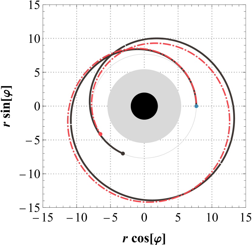
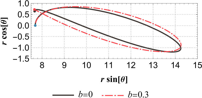
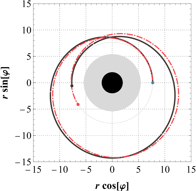
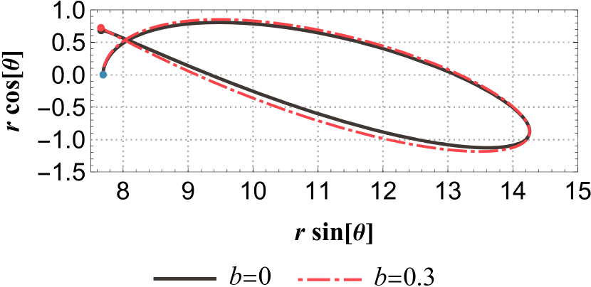
In Fig. 1, we plot the orbit over one radial period using the analytical solutions (98)-(101). The blue dot represents the starting point, while the red and black dots are the endpoints, but both at the periapsis. To display the effects of spin, we did not choose a small value of sโˆฅsubscript๐‘ parallel-tos_{\parallel} and sโŸ‚subscript๐‘ perpendicular-tos_{\perp}. As seen in Fig. 1, increasing in tidal charge $b$ reduces the periapsis precession angle, whereas increasing in spin enhances it.

VI Linear correction to the orbital frequencies

The linear correction to the Mino frequency reads

$\displaystyle\Upsilon^{r,t,\phi}$ $\displaystyle=$ ฮฅbr,t,ฯ•+sโˆฅโ€‹ฮดโ€‹ฮฅr,t,ฯ•.subscriptsuperscriptฮฅ๐‘Ÿ๐‘กitalic-ฯ•๐‘subscript๐‘ parallel-to๐›ฟsuperscriptฮฅ๐‘Ÿ๐‘กitalic-ฯ•\displaystyle\Upsilon^{r,t,\phi}_{b}+s_{\parallel}\delta\Upsilon^{r,t,\phi}. (106)

Here, $\Upsilon^{r,t,\phi}_{b}$ represents the geodesic Mino frequency without considering the spin of the test particle. Additionally, we can use the earlier expressions to reorganize the energy $\mathcal{E}^{2}$ (Eq.(57)), angular momentum $\mathcal{J}^{2}$ (Eq.(58)), and the roots $r_{3}$ (Eq.(75)) and $r_{4}$ (Eq.(75)) as:

$\displaystyle\mathcal{E}^{2}$ $\displaystyle=$ โ„ฐb2+sโˆฅโ€‹โ„ฐs2,superscriptsubscriptโ„ฐ๐‘2subscript๐‘ parallel-tosuperscriptsubscriptโ„ฐ๐‘ 2\displaystyle\mathcal{E}_{b}^{2}+s_{\parallel}\mathcal{E}_{s}^{2}, (107)
$\displaystyle\mathcal{J}^{2}$ $\displaystyle=$ ๐’ฅb2+sโˆฅโ€‹๐’ฅs2,superscriptsubscript๐’ฅ๐‘2subscript๐‘ parallel-tosuperscriptsubscript๐’ฅ๐‘ 2\displaystyle\mathcal{J}_{b}^{2}+s_{\parallel}\mathcal{J}_{s}^{2}, (108)
$\displaystyle r_{3}$ $\displaystyle=$ rbโ€‹3+sโˆฅโ€‹rsโ€‹3,subscript๐‘Ÿ๐‘3subscript๐‘ parallel-tosubscript๐‘Ÿ๐‘ 3\displaystyle r_{b3}+s_{\parallel}r_{s3}, (109)
$\displaystyle r_{4}$ $\displaystyle=$ rbโ€‹4+sโˆฅโ€‹rsโ€‹4.subscript๐‘Ÿ๐‘4subscript๐‘ parallel-tosubscript๐‘Ÿ๐‘ 4\displaystyle r_{b4}+s_{\parallel}r_{s4}. (110)

The other expressions without spin can be written as $k_{b}^{2}$, $h_{br}$, $h_{brp}$, $h_{brn}$, etc. For example,

$\displaystyle k_{b}^{2}=\frac{(r_{b1}-r_{b2})(r_{b3}-r_{b4})}{(r_{b1}-r_{b3})(r_{b2}-r_{b4})}.$ (111)

Therefore, $\Upsilon^{r}_{b}$ and its corresponding linear correction part $\delta\Upsilon^{r}$ can be described as

$\displaystyle\Upsilon^{r}_{b}$ $\displaystyle=$ $\displaystyle\frac{\pi\sqrt{1-\mathcal{E}_{b}^{2}}\sqrt{\left(r_{b1}-r_{b3}\right)\left(r_{b2}-r_{b4}\right)}}{2K_{e}[k_{b}^{2}]},$ (112)
$\displaystyle\delta\Upsilon^{r}$ $\displaystyle=$ $\displaystyle-\frac{\pi\sqrt{\left(r_{b1}-r_{b3}\right)\left(r_{b2}-r_{b4}\right)}}{4\sqrt{1-\mathcal{E}_{b}^{2}}K_{e}[k_{b}^{2}]^{2}\left(r_{b1}-r_{b4}\right)\left(r_{b3}-r_{b2}\right)\left(r_{b3}-r_{b4}\right)}$ (113)
$\displaystyle\Big{(}\left(\mathcal{E}_{b}^{2}-1\right)E_{e}[k_{b}^{2}]\left(r_{s4}\left(r_{b1}-r_{b3}\right)\left(r_{b3}-r_{b2}\right)+r_{s3}\left(r_{b1}-r_{b4}\right)\left(r_{b2}-r_{b4}\right)\right)$
$\displaystyle-K_{e}[k_{b}^{2}]\left(r_{b1}-r_{b4}\right)\left(r_{b2}-r_{b3}\right)\left(\left(\mathcal{E}_{b}^{2}-1\right)\left(r_{s3}-r_{s4}\right)+\mathcal{E}_{s}^{2}\left(r_{b3}-r_{b4}\right)\right)\Big{)}.$

When $b=0$, our results goes back to the corresponding formula in Ref. [30] with $k_{b}^{2}$ term becomes $k_{0}^{2}$. Similarly, the Mino frequencies for $\phi$ and $\psi$ are

$\displaystyle\Upsilon^{\phi}_{b}$ $\displaystyle=$ $\displaystyle\mathcal{J}_{b},$ (114)
$\displaystyle\delta\Upsilon^{\phi}$ $\displaystyle=$ ๐’ฅs22โ€‹๐’ฅb+โ„ฐb,superscriptsubscript๐’ฅ๐‘ 22subscript๐’ฅ๐‘subscriptโ„ฐ๐‘\displaystyle\frac{\mathcal{J}_{s}^{2}}{2\mathcal{J}_{b}}+\mathcal{E}_{b}, (115)
$\displaystyle\Upsilon^{\psi}_{b}$ $\displaystyle=$ $\displaystyle\frac{\mathcal{E}_{b}\mathcal{J}_{b}r_{b3}^{2}}{\mathcal{J}_{b}^{2}+r_{b3}^{2}}+\frac{\mathcal{E}_{b}\mathcal{J}_{b}^{2}\left(r_{b2}-r_{b3}\right)}{\left(\mathcal{J}_{b}^{2}+r_{b2}^{2}\right)\left(\mathcal{J}_{b}^{2}+r_{b3}^{2}\right)K_{e}[k_{b}^{2}]}$ (116)
((rbโ€‹2rbโ€‹3โˆ’๐’ฅb2)Im[ฮ e[(rbโ€‹1โˆ’rbโ€‹2)โ€‹(rbโ€‹3โˆ’iโ€‹๐’ฅb)(rbโ€‹1โˆ’rbโ€‹3)โ€‹(rbโ€‹2โˆ’iโ€‹๐’ฅb),kb2]]\displaystyle\bigg{(}\left(r_{b2}r_{b3}-\mathcal{J}_{b}^{2}\right)\mathrm{Im}\left[\Pi_{e}\left[\frac{\left(r_{b1}-r_{b2}\right)\left(r_{b3}-i\mathcal{J}_{b}\right)}{\left(r_{b1}-r_{b3}\right)\left(r_{b2}-i\mathcal{J}_{b}\right)},k_{b}^{2}\right]\right]
+๐’ฅb(rbโ€‹2+rbโ€‹3)Re[ฮ e[(rbโ€‹1โˆ’rbโ€‹2)โ€‹(rbโ€‹3โˆ’iโ€‹๐’ฅb)(rbโ€‹1โˆ’rbโ€‹3)โ€‹(rbโ€‹2โˆ’iโ€‹๐’ฅb),kb2]]).\displaystyle+\mathcal{J}_{b}\left(r_{b2}+r_{b3}\right)\mathrm{Re}\left[\Pi_{e}\left[\frac{\left(r_{b1}-r_{b2}\right)\left(r_{b3}-i\mathcal{J}_{b}\right)}{\left(r_{b1}-r_{b3}\right)\left(r_{b2}-i\mathcal{J}_{b}\right)},k_{b}^{2}\right]\right]\bigg{)}.

Then, we can obtain the the nodal precession $\nu_{nodal}$ and the periastron precession $\nu_{peri}$ as

$\displaystyle\nu_{nodal}$ $\displaystyle=$ $\displaystyle 2\pi\left(\frac{\Upsilon^{\phi}_{b}}{\Upsilon^{\psi}_{b}}-1\right),$ (117)
$\displaystyle\nu_{peri}$ $\displaystyle=$ ฮฝpโ€‹eโ€‹rโ€‹ib+ฮฝpโ€‹eโ€‹rโ€‹isโ€‹sโˆฅ=2โ€‹ฯ€โ€‹(ฮฅbฯ•ฮฅbrโˆ’1)+2โ€‹ฯ€โ€‹ฮฅbrโ€‹ฮดโ€‹ฮฅฯ•โˆ’ฮดโ€‹ฮฅrโ€‹ฮฅbฯ•(ฮฅbr)2โ€‹sโˆฅ.subscriptsuperscript๐œˆ๐‘๐‘๐‘’๐‘Ÿ๐‘–subscriptsuperscript๐œˆ๐‘ ๐‘๐‘’๐‘Ÿ๐‘–subscript๐‘ parallel-to2๐œ‹subscriptsuperscriptฮฅitalic-ฯ•๐‘subscriptsuperscriptฮฅ๐‘Ÿ๐‘12๐œ‹subscriptsuperscriptฮฅ๐‘Ÿ๐‘๐›ฟsuperscriptฮฅitalic-ฯ•๐›ฟsuperscriptฮฅ๐‘Ÿsubscriptsuperscriptฮฅitalic-ฯ•๐‘superscriptsubscriptsuperscriptฮฅ๐‘Ÿ๐‘2subscript๐‘ parallel-to\displaystyle\nu^{b}_{peri}+\nu^{s}_{peri}s_{\parallel}=2\pi\left(\frac{\Upsilon^{\phi}_{b}}{\Upsilon^{r}_{b}}-1\right)+2\pi\frac{\Upsilon^{r}_{b}\delta\Upsilon^{\phi}-\delta\Upsilon^{r}\Upsilon^{\phi}_{b}}{\left(\Upsilon^{r}_{b}\right)^{2}}s_{\parallel}. (118)

From Eq.(117), we consider the spinless part of $\nu_{nodal}$. This is because, from Eq.(40), nodal precession is only an ๐’ชโ€‹[s]๐’ชdelimited-[]๐‘ \mathcal{O}[s] order effect. In contrast, periastron precession requires up to the linear order in spin.

Refer to caption
(a) $e=0.3$ and $p=10$
Refer to caption
(b) $e=0.3$ and $p=10$
Figure 2: Nodal and periastron precession under different tidal charge $b$ and spin sโˆฅsubscript๐‘ parallel-tos_{\parallel}.

The nodal and the periastron precession for different values of $b$ and sโˆฅsubscript๐‘ parallel-tos_{\parallel} is illustrated in Fig. 2. From Fig. 2, it can be seen that periapsis precession increases as the tidal charge $b$ decreases and sโˆฅsubscript๐‘ parallel-tos_{\parallel} increases. This is consistent with the conclusions from Fig. 1.

VII Conclusion

In this paper, we considered the explicit orbital solutions for the motion of a spinning test particle in the brane-world spacetime. Along the line of [30], we first analyzed the equations of motion for the test spinning particle, then provided the evolution of the spin components through parallel transport. Next, we derived the Keplerian parameter expressions for the energy and angular momentum, as well as the four roots of the radial velocity. As a result, we presented the elliptical integral calculation of the equations of motion in the Carter-Mino time and obtained the linear shift of the orbital frequency. The influences of different value of tidal charge $b$ or spin sโˆฅsubscript๐‘ parallel-tos_{\parallel} on the orbit in the angular-momentum-aligned coordinates has depicted in Fig. 1. Moreover, we found that both the nodal precession and the periastron precession become larger when the tidal charge $b$ of brane-world spacetime becomes smaller. For the periastron precession, the effect will be further amplified as the spin increases.

There are a lot of works that deserve further investigation. For example, it is interesting to extend these results to the case of Reissner-Nordstrom spacetime with neutral or charged test particles. In such a scenario, the test particle will not only be subject to the spin-curvature force but also the electromagnetic interaction force. Additionally, we anticipate using the conclusions derived from this method to study gravitational waveforms in EMRI systems.

Acknowledgements.
Some of this work make use of xAct[54]. This work is supported by National Natural Science Foundation of China (NSFC) with Grants No. 12275087.

Appendix A Effective potential and bound orbits

The effective potential $V_{eff}$ can be defined as [52, 42]

$\displaystyle V_{eff}$ $\displaystyle=$ $\displaystyle\mathcal{E}^{2}-\dot{r}^{2}$ (119)
$\displaystyle=$ (๐’ฅ2+r2)โ€‹fโ€‹[r]r2+๐’ฅโ€‹โ„ฐโ€‹(2โ€‹fโ€‹[r]โˆ’rโ€‹fโ€ฒโ€‹[r])โ€‹sโˆฅr2.superscript๐’ฅ2superscript๐‘Ÿ2๐‘“delimited-[]๐‘Ÿsuperscript๐‘Ÿ2๐’ฅโ„ฐ2๐‘“delimited-[]๐‘Ÿ๐‘Ÿsuperscript๐‘“โ€ฒdelimited-[]๐‘Ÿsubscript๐‘ parallel-tosuperscript๐‘Ÿ2\displaystyle\frac{(\mathcal{J}^{2}+r^{2})f[r]}{r^{2}}+\frac{\mathcal{J}\mathcal{E}(2f[r]-rf^{\prime}[r])s_{\parallel}}{r^{2}}.

We can see that, unlike the spinless case, the inclusion of spin effects introduces a coupling term ๐’ฅโ€‹โ„ฐโ€‹sโˆฅ๐’ฅโ„ฐsubscript๐‘ parallel-to\mathcal{J}\mathcal{E}s_{\parallel} and implies that changing the energy $\mathcal{E}$ does not simply translate the effective potential up or down. This feature makes finding analytical solutions for marginally bound orbits (MBO) and innermost stable circular orbits (ISCO) more complex.

For MBO, the condition is

$\displaystyle V_{eff}[r_{MBO}]=1,\quad V^{\prime}_{eff}[r_{MBO}]=0,$ (120)

while for ISCO, the condition becomes

$\displaystyle V_{eff}[r_{ISCO}]=\mathcal{E}^{2},\quad V^{\prime}_{eff}[r_{ISCO}]=0,\quad V^{\prime\prime}_{eff}[r_{ISCO}]=0.$ (121)

The numerical results are shown in Fig. 3.

Refer to caption
(a) sโˆฅ=0.2subscript๐‘ parallel-to0.2s_{\parallel}=0.2, $b=-1$
Refer to caption
(b) sโˆฅ=0.2subscript๐‘ parallel-to0.2s_{\parallel}=0.2, $b=0$
Refer to caption
(c) sโˆฅ=0.2subscript๐‘ parallel-to0.2s_{\parallel}=0.2, $b=1$
Refer to caption
(d) sโˆฅ=โˆ’0.2subscript๐‘ parallel-to0.2s_{\parallel}=-0.2, $b=-1$
Refer to caption
(e) sโˆฅ=โˆ’0.2subscript๐‘ parallel-to0.2s_{\parallel}=-0.2, $b=0$
Refer to caption
(f) sโˆฅ=โˆ’0.2subscript๐‘ parallel-to0.2s_{\parallel}=-0.2, $b=1$
Figure 3: The effective potential $V_{eff}[r]$ for different values of sโˆฅsubscript๐‘ parallel-tos_{\parallel} and $b$. The Energy $\mathcal{E}$ and angular momentum $\mathcal{J}$ varies from $\{\mathcal{E}_{ISO},\mathcal{J}_{ISO}\}$ to $\{\mathcal{E}_{MBO},\mathcal{J}_{MBO}\}$ from bottom to top. The dashed orange line is located at the extremal points of $V_{eff}[r]$. The gray area on the left represents the part that inside the event horizon.

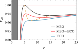
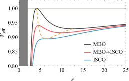
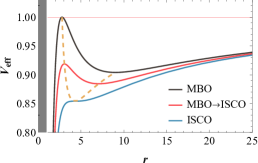
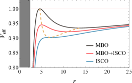
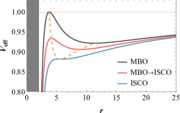
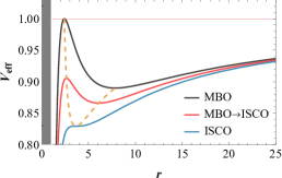
From Fig. 3, the radius of ISO (MBO) decreases as the tidal charge $b$ increases while as the sโˆฅsubscript๐‘ parallel-tos_{\parallel} increases, the radius of ISO (MBO) increases.

On the other hand, we have the expressions for the roots in Sec. IV.2. Therefore, ISO can also be found by setting $r_{2}=r_{3}$. However, even in the absence of spin effects, the analytical result for the ISO in the brane-world remains quite complex.

Refer to caption
Figure 4: The semilatus rectum $p$ of the ISO as functions of the tidal charge $b$ for different values of sโˆฅsubscript๐‘ parallel-tos_{\parallel}, with $e=0.1$.

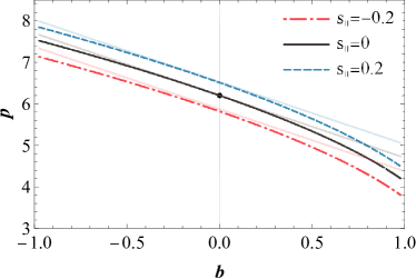
Hence, in Fig. 4, we obtained the semilatus rectum $p$ of the ISO numerically. Then {b,sโˆฅ,e}๐‘subscript๐‘ parallel-to๐‘’\{b,s_{\parallel},e\} as small quantities, we can obtain the approximation

p=6+2โ€‹eโˆ’3โ€‹b2+2โ€‹23โ€‹sโˆฅ.๐‘62๐‘’3๐‘2223subscript๐‘ parallel-to\displaystyle p=6+2e-\frac{3b}{2}+2\sqrt{\frac{2}{3}}s_{\parallel}. (122)

As Fig. 4 shows, when $e$, $b$ and sโˆฅsubscript๐‘ parallel-tos_{\parallel} approach to zero, the light line representing the approximate result approaches the numerical one. This approximate result is consistent with Eq.(B19) in [26]. It can be seen that the $p$ of the ISO decreases with increasing $b$ and decreasing sโˆฅsubscript๐‘ parallel-tos_{\parallel}. This is in contrast to the conclusion in [53], where the ISCO ($e=0$) decreases with increasing spin s๐‘ s. This discrepancy arises because the second leg in the Marck tetrad has an opposite sign compared to the second basis in the tetrad used in [53].

Appendix B Formulae of integrals of radial motion

$F_{e}[\chi,k^{2}]$, $E_{e}[\chi,k^{2}]$, and ฮ eโ€‹[n,ฯ‡,k2]subscriptฮ ๐‘’๐‘›๐œ’superscript๐‘˜2\Pi_{e}[n,\chi,k^{2}] are the elliptic integrals of the first, second, and third kinds, respectively, as follows [53].

$\displaystyle F_{e}[\chi,k^{2}]$ $\displaystyle=$ $\displaystyle\int_{0}^{\chi}(1-k^{2}\sin^{2}[\theta])^{-1/2}d\theta,$ (123)
$\displaystyle E_{e}[\chi,k^{2}]$ $\displaystyle=$ $\displaystyle\int_{0}^{\chi}(1-k^{2}\sin^{2}[\theta])^{1/2}d\theta,$ (124)
ฮ eโ€‹[n,ฯ‡,k2]subscriptฮ ๐‘’๐‘›๐œ’superscript๐‘˜2\displaystyle\Pi_{e}[n,\chi,k^{2}] $\displaystyle=$ $\displaystyle\int_{0}^{\chi}(1-k^{2}\sin^{2}[\theta])^{-1/2}(1-n\sin^{2}[\theta])^{-1}d\theta.$ (125)

The corresponding complete elliptic integrals are given by

$\displaystyle K_{e}[k^{2}]$ $\displaystyle=$ $\displaystyle F_{e}[\pi/2,k^{2}],$ (126)
$\displaystyle E_{e}[k^{2}]$ $\displaystyle=$ $\displaystyle E_{e}[\pi/2,k^{2}],$ (127)
ฮ eโ€‹[n,k2]subscriptฮ ๐‘’๐‘›superscript๐‘˜2\displaystyle\Pi_{e}[n,k^{2}] $\displaystyle=$ ฮ eโ€‹[n,ฯ€/2,k2].subscriptฮ ๐‘’๐‘›๐œ‹2superscript๐‘˜2\displaystyle\Pi_{e}[n,\pi/2,k^{2}]. (128)

The inverses of the $F_{e}[\chi,k^{2}]$ is

$\displaystyle F_{e}[\mathrm{am}[y,k^{2}],k^{2}]$ $\displaystyle=$ $\displaystyle y,$ (129)
$\displaystyle\mathrm{sn}[y,k^{2}]$ $\displaystyle=$ $\displaystyle\sin[\mathrm{am}[y,k^{2}]].$ (130)

Appendix C The result for Schwarzschild case

In the Schwarzschild case, we obtained the following result as

$\displaystyle\Upsilon^{t}_{Sh}$ $\displaystyle=$ $\displaystyle\frac{\mathcal{E}}{2K_{e}[k^{2}]}\bigg{(}\frac{2\left(r_{1}-r_{3}\right)\left(r_{2}-r_{3}\right)+r_{3}\left(r_{1}\left(r_{3}-r_{2}\right)+r_{3}\left(r_{2}+r_{3}\right)\right)}{r_{3}-2}K_{e}[k^{2}]$ (131)
+(r2โˆ’r3)โ€‹(r1+r2+r3+4)โ€‹ฮ eโ€‹[r1โˆ’r2r1โˆ’r3,k2]+r2โ€‹(r1โˆ’r3)โ€‹Eeโ€‹[k2]subscript๐‘Ÿ2subscript๐‘Ÿ3subscript๐‘Ÿ1subscript๐‘Ÿ2subscript๐‘Ÿ34subscriptฮ ๐‘’subscript๐‘Ÿ1subscript๐‘Ÿ2subscript๐‘Ÿ1subscript๐‘Ÿ3superscript๐‘˜2subscript๐‘Ÿ2subscript๐‘Ÿ1subscript๐‘Ÿ3subscript๐ธ๐‘’delimited-[]superscript๐‘˜2\displaystyle+\left(r_{2}-r_{3}\right)\left(r_{1}+r_{2}+r_{3}+4\right)\Pi_{e}\left[\frac{r_{1}-r_{2}}{r_{1}-r_{3}},k^{2}\right]+r_{2}\left(r_{1}-r_{3}\right)E_{e}[k^{2}]
+16โ€‹(r2โˆ’r3)(r2โˆ’2)โ€‹(2โˆ’r3)โ€‹ฮ eโ€‹[(r1โˆ’r2)โ€‹(r3โˆ’2)(r1โˆ’r3)โ€‹(r2โˆ’2),k2]16subscript๐‘Ÿ2subscript๐‘Ÿ3subscript๐‘Ÿ222subscript๐‘Ÿ3subscriptฮ ๐‘’subscript๐‘Ÿ1subscript๐‘Ÿ2subscript๐‘Ÿ32subscript๐‘Ÿ1subscript๐‘Ÿ3subscript๐‘Ÿ22superscript๐‘˜2\displaystyle+\frac{16\left(r_{2}-r_{3}\right)}{\left(r_{2}-2\right)\left(2-r_{3}\right)}\Pi_{e}\left[\frac{\left(r_{1}-r_{2}\right)\left(r_{3}-2\right)}{\left(r_{1}-r_{3}\right)\left(r_{2}-2\right)},k^{2}\right]
โˆ’๐’ฅโ€‹sโˆฅโ„ฐ(2โ€‹(r3โˆ’r2)(r2โˆ’2)โ€‹(2โˆ’r3)ฮ e[(r1โˆ’r2)โ€‹(r3โˆ’2)(r1โˆ’r3)โ€‹(r2โˆ’2),k2]+2โ€‹Keโ€‹[k2](2โˆ’r3))).\displaystyle-\frac{\mathcal{J}s_{\parallel}}{\mathcal{E}}\left(\frac{2\left(r_{3}-r_{2}\right)}{\left(r_{2}-2\right)\left(2-r_{3}\right)}\Pi_{e}\left[\frac{\left(r_{1}-r_{2}\right)\left(r_{3}-2\right)}{\left(r_{1}-r_{3}\right)\left(r_{2}-2\right)},k^{2}\right]+\frac{2K_{e}[k^{2}]}{\left(2-r_{3}\right)}\right)\bigg{)}.

References

  • [1] B.P. Abbott, et al. (LIGO Scientific and Virgo Collaborations), Observation of Gravitational Waves from a Binary Black Hole Merger, Phys. Rev. Lett. 116, 061102 (2016).
  • [2] R. Abbott, et al. (LIGO Scientific and Virgo Collaborations), GWTC-2: Compact Binary Coalescences Observed by LIGO and Virgo during the First Half of the Third Observing Run, Phys. Rev. X 11, 021053 (2021).
  • [3] R. Abbott, et al. (LIGO Scientific, Virgo and KAGRA Collaborations), GWTC-3: Compact Binary Coalescences Observed by LIGO and Virgo during the Second Part of the Third Observing Run, Phys. Rev. X 13, 041039 (2023).
  • [4] R. Abbott, et al. (LIGO Scientific and Virgo Collaborations), GWTC-2.1: Deep Extended Catalog of Compact Binary Coalescences Observed by LIGO and Virgo during the First Half of the Third Observing Run, Phys. Rev. D 109, 022001 (2024).
  • [5] P. Amaro-Seoane et al., Laser Interferometer Space Antenna, arXiv:1702.00786.
  • [6] G. Wang, W.-T. Ni, W.-B. Han, P. Xu, and Z. Luo, Alternative LISA-TAIJI Networks, Phys. Rev. D 104, 024012 (2021).
  • [7] W.-R. Hu and Y.-L. Wu, The Taiji Program in Space for Gravitational Wave Physics and the Nature of Gravity, National Science Review 4, 685 (2017).
  • [8] J. Mei et al., The TianQin Project: Current Progress on Science and Technology, Progress of Theoretical and Experimental Physics 2021, 05A107 (2021).
  • [9] S. Babak, J. Gair, A. Sesana, E. Barausse, C. F. Sopuerta, C. P. L. Berry, E. Berti, P. Amaro-Seoane, A. Petiteau, and A. Klein, Science with the Space-Based Interferometer LISA. V. Extreme Mass-Ratio Inspirals, Phys. Rev. D 95, 103012 (2017).
  • [10] K. G. Arun et al., New Horizons for Fundamental Physics with LISA, Living Rev Relativ 25, 4 (2022).
  • [11] S. A. Hughes, S. Drasco, E.E. Flanagan, and J. Franklin, Gravitational Radiation Reaction and Inspiral Waveforms in the Adiabatic Limit, Phys. Rev. Lett. 94, 221101 (2005).
  • [12] S. A. Hughes, N. Warburton, G. Khanna, A. J. K. Chua, and M. L. Katz, Adiabatic Waveforms for Extreme Mass-Ratio Inspirals via Multivoice Decomposition in Time and Frequency, Phys. Rev. D 103, 104014 (2021).
  • [13] B. Wardell, A. Pound, N. Warburton, J. Miller, L. Durkan, and A. Le Tiec, Gravitational Waveforms for Compact Binaries from Second-Order Self-Force Theory, Phys. Rev. Lett. 130, 241402 (2023).
  • [14] E. A. Huerta, J. R. Gair, and D. A. Brown, Importance of Including Small Body Spin Effects in the Modelling of Intermediate Mass-Ratio Inspirals. II. Accurate Parameter Extraction of Strong Sources Using Higher-Order Spin Effects, Phys. Rev. D 85, 064023 (2012).
  • [15] G. A. Piovano, R. Brito, A. Maselli, and P. Pani, Assessing the Detectability of the Secondary Spin in Extreme Mass-Ratio Inspirals with Fully Relativistic Numerical Waveforms, Phys. Rev. D 104, 124019 (2021).
  • [16] D. Gerosa, M. Kesden, R. Oโ€™ Shaughnessy, A. Klein, E. Berti, U. Sperhake, and D. Trifiro, Precessional Instability in Binary Black Holes with Aligned Spins, Phys. Rev. Lett. 115, 141102 (2015).
  • [17] D. Gerosa, M. Kesden, U. Sperhake, E. Berti, and R. Oโ€™ Shaughnessy, Multi-Timescale Analysis of Phase Transitions in Precessing Black-Hole Binaries, Phys. Rev. D 92, 064016 (2015).
  • [18] M. Kesden, D. Gerosa, R. Oโ€™ Shaughnessy, E. Berti, and U. Sperhake, Effective Potentials and Morphological Transitions for Binary Black Hole Spin Precession, Phys. Rev. Lett. 114, 081103 (2015).
  • [19] M. Mould and D. Gerosa, Endpoint of the Up-down Instability in Precessing Binary Black Holes, Phys. Rev. D 101, 124037 (2020).
  • [20] S. Tanay, L. C. Stein, and J. T. Galvez Ghersi, Integrability of Eccentric, Spinning Black Hole Binaries up to Second Post-Newtonian Order, Phys. Rev. D 103, 064066 (2021).
  • [21] G. Fumagalli and D. Gerosa, Spin-Eccentricity Interplay in Merging Binary Black Holes, Phys. Rev. D 108, 124055 (2023).
  • [22] S. Tanay, L. C. Stein, and G. Cho, Action-Angle Variables of a Binary Black Hole with Arbitrary Eccentricity, Spins, and Masses at 1.5 Post-Newtonian Order, Phys. Rev. D 107, 103040 (2023).
  • [23] T. Damour, Coalescence of Two Spinning Black Holes: An Effective One-Body Approach, Phys. Rev. D 64, 124013 (2001).
  • [24] S. Balmelli and P. Jetzer, Effective-One-Body Hamiltonian with next-to-Leading Order Spin-Spin Coupling for Two Nonprecessing Black Holes with Aligned Spins, Phys. Rev. D 87, 124036 (2013).
  • [25] S. Balmelli and P. Jetzer, Effective-One-Body Hamiltonian with next-to-Leading Order Spin-Spin Coupling, Phys. Rev. D 91, 064011 (2015).
  • [26] M. Favata, Conservative Corrections to the Innermost Stable Circular Orbit (ISCO) of a Kerr Black Hole: A New Gauge-Invariant Post-Newtonian ISCO Condition, and the ISCO Shift Due to Test-Particle Spin and the Gravitational Self-Force, Phys. Rev. D 83, 024028 (2011).
  • [27] S. Mukherjee, Collisional Penrose Process with Spinning Particles, Physics Letters B 778, 54 (2018).
  • [28] M. Guo and S. Gao, Kerr Black Holes as Accelerators of Spinning Test Particles, Phys. Rev. D 93, 084025 (2016).
  • [29] M. Rahman and A. Bhattacharyya, Prospects for Determining the Nature of the Secondaries of Extreme Mass-Ratio Inspirals Using the Spin-Induced Quadrupole Deformation, Phys. Rev. D 107, 024006 (2023).
  • [30] V. Witzany and G. A. Piovano, Analytic Solutions for the Motion of Spinning Particles near Spherically Symmetric Black Holes and Exotic Compact Objects, Phys. Rev. Lett. 132, 171401 (2024).
  • [31] T. Hinderer et al., Periastron Advance in Spinning Black Hole Binaries: Comparing Effective-One-Body and Numerical Relativity, Phys. Rev. D 88, 084005 (2013).
  • [32] L. V. Drummond and S. A. Hughes, Precisely Computing Bound Orbits of Spinning Bodies around Black Holes. I. General Framework and Results for Nearly Equatorial Orbits, Phys. Rev. D 105, 124040 (2022).
  • [33] L. V. Drummond and S. A. Hughes, Precisely Computing Bound Orbits of Spinning Bodies around Black Holes. II. Generic Orbits, Phys. Rev. D 105, 124041 (2022).
  • [34] O. Klein, Quantum theory and five-dimensional theory of relativity. Z. Phys. 37 (1926) (in German and English)
  • [35] T.H. Kaluza, On the unification problem in physics. Int. J. Mod. Phys. D 27, 1870001 (2018)
  • [36] T. Shiromizu, K. Maeda, and M. Sasaki, The Einstein Equations on the 3-Brane World, Phys. Rev. D 62, (2000).
  • [37] R. Maartens and K. Koyama, Brane-World Gravity, Living Rev. Relativ. 13, 5 (2010).
  • [38] N. Dadhich, R. Maartens, P. Papadopoulos, and V. Rezania, Black Holes on the Brane, Physics Letters B 487, 1 (2000).
  • [39] I. Stojiljkovic, D. Dordevic, A. Gocanin, and D. Gocanin, Testing the Braneworld Theory with Identical Particles, Phys. Rev. D 108, 124008 (2023).
  • [40] Y. Du, Y. Liu, and X. Zhang, Collisional Penrose Process of Braneworld Black Hole with Spinning Particles, Eur. Phys. J. C 82, 871 (2022).
  • [41] U. Nucamendi, R. Becerril, and P. Sheoran, Bounds on Spinning Particles in Their Innermost Stable Circular Orbits around Rotating Braneworld Black Hole, Eur. Phys. J. C 80, 35 (2020).
  • [42] X.-M. Deng, Periodic Orbits around Brane-World Black Holes, Eur. Phys. J. C 80, 489 (2020).
  • [43] A. Papapetrou, Spinning Test Particles in General Relativity. I, Proc. Roy. Soc. Lond. A 209, 248 (1951).
  • [44] W. G. Dixon and H. Bondi, Dynamics of Extended Bodies in General Relativity. I. Momentum and Angular Momentum, Proc. Roy. Soc. Lond. A 314, 499 (1970).
  • [45] W. G. Dixon and A. Hewish, Dynamics of Extended Bodies in General Relativity. II. Moments of the Charge-Current Vector, Proc. Roy. Soc. Lond. A 319, 509 (1970).
  • [46] T. W, Motion of Multipole Particles in General Relativity Theory, Acta Phys Pol 18, 393 (1959).
  • [47] J.-A. Marck, Solution to the Equations of Parallel Transport in Kerr Geometry; Tidal Tensor, Proceedings of the Royal Society of London. Series A, Mathematical and Physical Sciences 385, 431 (1983).
  • [48] M. van de Meent, Analytic Solutions for Parallel Transport along Generic Bound Geodesics in Kerr Spacetime, Class. Quantum Grav. 37, 145007 (2020).
  • [49] C. G. Darwin, The Gravity Field of a Particle, Proceedings of the Royal Society of London. Series A. Mathematical and Physical Sciences 249, 180 (1959).
  • [50] B. Carter, Hamilton-Jacobi and Schrodinger Separable Solutions of Einsteinโ€™s Equations, Communications in Mathematical Physics 10, 280 (1968).
  • [51] Y. Mino, Perturbative Approach to an Orbital Evolution around a Supermassive Black Hole, Phys. Rev. D 67, 084027 (2003).
  • [52] W. Rindler, Relativity: Special, General, And Cosmological Second Edition (Oxford University Press, 2006).
  • [53] Y.-P. Zhang, S.-W. Wei, W.-D. Guo, T.-T. Sui, and Y.-X. Liu, Innermost Stable Circular Orbit of Spinning Particle in Charged Spinning Black Hole Background, Phys. Rev. D 97, 084056 (2018).
  • [54] J. M. Martรญn-Garcรญa, xAct: Efficient tensor computer algebra for the Wolfram Language, http://www.xact.es/