Deep reinforcement learning for the management of the wall regeneration cycle in wall-bounded turbulent flows

Abstract

The wall cycle in wall-bounded turbulent flows is a complex turbulence regeneration mechanism that remains not fully understood. This study explores the potential of deep reinforcement learning (DRL) for managing the wall regeneration cycle to achieve desired flow dynamics. We integrate the StableBaselines3 DRL libraries with the open-source DNS solver CaNS to create a robust platform for dynamic flow control. The DRL agent interacts with the DNS environment, learning policies that modify wall boundary conditions to optimize objectives such as the reduction of the skin-friction coefficient or the enhancement of certain coherent structures features.

Initial experiments demonstrate the capability of DRL to achieve drag-reduction rates comparable with those achieved via traditional methods, though limited to short time periods. We also propose a strategy to enhance the coherence of velocity streaks, assuming that maintaining straight streaks can inhibit instability and further reduce skin friction. The implementation makes use of the message-passing-interface (MPI) wrappers for efficient communication between the Python-based DRL agent and the DNS solver, ensuring scalability on high-performance computing architectures.

Our results highlight the promise of DRL in flow control applications and underscore the need for more advanced control laws and objective functions. Future work will focus on optimizing actuation periods and exploring new computational architectures to extend the applicability and the efficiency of DRL in turbulent flow management.

1 Introduction

The wall cycle [13] in wall-bounded turbulent flows is a turbulence regenerating mechanism whose dynamics are still not fully understood. Understanding and controlling the wall-cycle is a technological challenge primarily pursued to either reduce the skin-friction coefficient or to achieve a desired impact on flow dynamics (e.g. enhancement of heat and mass transfer).

Active flow control techniques are among the most promising methodologies to manipulate the near wall flow for technological benefits because of their ability to work with closed-loop feedback and handle off-design conditions. However, their complexity currently limits real-world application. One such technique is based on the use of Streamwise Travelling Waves (STW) of spanwise velocity [24], which involves applying a sinusoidal wave with a time-dependent pulsation as a boundary condition for the spanwise velocity $w$ at the wall. The use of this method can lead to skin friction coefficient $C_{f}$ reduction by up to $45\%$ [24]. However, the definition of a particular STW leading to the highest drag reduction requires a computationally expensive analysis of the parametric space at hand, defined by the frequency and spatial wavenumber of the travelling wave

Deep Reinforcement Learning (DRL) [18][19] offers a potential breakthrough by overcoming the limitations of standard parametric studies, enhancing existing flow control techniques, and allowing for dynamic variations of the parameters. In general, in fluid dynamics-related contexts, DRL involves the interaction of an agent with a physical environment, as depicted in figure 1. The agent, built upon a neural network, lacks prior knowledge of the physical phenomena occurring in the environment. Using on-policy algorithms, such as Proximal Policy Optimization (PPO) [26], the agent receives an input (often called the state) in the form of data from the environment, termed an observation, which is a partial representation of the system state. The reward, a scalar value associated with the observation, is high when the observation corresponds to a desired configuration and low otherwise. The output, or action(s), consists of parameters that modify conditions within the environment.

When the environment (e.g. the DNS of a turbulent flow) receives a new set of actions, the physics of the flow are simulated to produce a new observation and its associated reward. This process changes the agent’s state and updates the weights of the neural network based on the current reward and the policy used. These updated weights generate new actions that modify the environment, triggering a new step. Multiple steps constitute an episode, and the agent continuously performs steps to maximize the reward over each episode.

In this work, an agent is trained to gather observations from a Direct Numerical Simulation (DNS) (the environment) of a plane, turbulent channel flow and apply a time-dependent action that dynamically modifies the wall boundary conditions, ultimately pursuing a policy that maximises a given the reward.

We will be looking at two different rewards: one is related to the minimisation of $C_{f}$, the other to the promotion of highly elongated velocity streaks.

This second choice is motivated by the intention of understanding how the topology of coherent structures impacts the development of the wall regeneration cycle. This involves promoting specific topologies of the flow, which helps infer the causality between the control law and its effect on the turbulent wall-cycle by linking the straightening of streaks to the reduction of $C_{f}$ Further efforts will focus on this direction by testing alternative objective functions that target specific features of the wall cycle.

From an implementation perspective, this work involved integrating the StableBaselines3 DRL libraries [25] with the open-source DNS solver CaNS [4]. The final interface is based on an ad-hoc MPI implementation, where a Python code invokes the execution of the DNS code on a set of processors and manages the communication with the DRL library. While the most common choice is resorting to Python codes both for the DNS and the DRL routines (see for example [28]), similar unconventional couplings become necessary when the 3D turbulent DNS requires more tailored codes not to waste computational resources, like in the work of [9], [27] and [7]. Alternatives that are simpler to implement have been explored, such as DNS codes being asked to save data on disk, rather than keeping it in memory, with bash scripts orchestrating the various calls of the DRL training and the DNS code to produce new data. This method has been initially implemented with a reliable DNS in-house developed solver, SUSA [22][21], but it has later been discontinued, due to the high inefficiency of the coupling itself.

The initial results indicate the need for more advanced control laws to fully exploit the tools developed in these early experiments. Currently, DRL agents are trained to find a control law based on a single dynamic parameter, but better policies could emerge from more complex control laws involving multiple dynamic parameters.

2 Methodology

2.1 Deep Reinforcement Learning

Figure 1: Schematic representation of the interaction between the DRL agent and the DNS environment.

As mentioned, in the present context, DRL-based flow control consists in the interaction of an agent with a turbulent channel flow modeled through a DNS, as depicted in figure 1.

The agents aims at learning a policy $\pi_{\theta}(a|s)$ that represents the probability of taking action $a$ in state $s$ given neural network parameters $\theta$. The interaction with the environment finds a trajectory $\{(s_{t},a_{t},r_{t},s_{t+1})\}$ in the state-action space that depends on the old policy. The agent then evaluates the advantage function $A_{t}$, that measures how good an action is compared to the average action at a given state. $A_{t}$ is typically defined as:

$$A_{t}=Q(s_{t},a_{t})-V(s_{t})$$ (1)

where $Q(s_{t},a_{t})$ is the action-value function and $V(s_{t})$ is the value function. The policy parameters $\theta$ are then updated to minimise the loss function $L(\theta)$, defined as

$$L(\theta)=\mathbb{E}_{t}\left[L^{CLIP}(\theta)-c_{1}L^{VF}(\theta)+c_{2}S[\pi_{\theta}](s_{t})\right],$$ (2)

with

$$L^{CLIP}(\theta)=\mathbb{E}_{t}\left[\min\left(r_{t}(\theta)A_{t},\text{clip}(r_{t}(\theta),1-\epsilon,1+\epsilon)A_{t}\right)\right],$$ (3)

and

$$L^{VF}(\theta)=\mathbb{E}_{t}\left[\left(V_{\theta}(s_{t})-V_{t}^{\text{target}}\right)^{2}\right],$$ (4)

where $r_{t}(\theta)=\frac{\pi_{\theta}(a_{t}|s_{t})}{\pi_{\theta_{old}}(a_{t}|s_{t})}$ is the probability ratio and $\epsilon$ is a hyperparameter that controls the clipping range, $V_{t}^{\text{target}}$ is typically computed as the discounted sum of rewards plus the bootstrapped value from the next state, $c_{1}$ and $c_{2}$ are coefficients that balance the contributions of the value function loss and the entropy bonus, which is defined as

$$S[\pi](s)=-\sum_{a}\pi(a|s)\log\pi(a|s).$$ (5)

When the agent is trained the policy will be able to choose a given action $a$ from a stochastic distribution parametrised by $\theta$ that will maximise the reward based on the trajectory it received.

The input data from DNS can have any structure, as long as the neural network (NN) is built with matrices of compatible sizes for multiplication. Inputs can be array-like, and in such cases, the most common policy adopted is the Multi-Input Policy (MLP) [20], which learns to weigh each input based on its relevance to the task, but it does not explicitly model any interdependencies between input features. However, in our specific application, it is crucial to preserve the spatial correlation of the input, as any combinations of sampled instantaneous quantities from a flow field are linked by the Navier-Stokes equations. Therefore, 2D, black and white, images rather than one-dimensional arrays of data are fed to the neural network. When using an image as input, the colour of a given pixel is not necessarily uncorrelated with the colours of other pixels.

By using images, we can effectively exploit the features of convolutional neural networks (CNNs) [16][17] without losing information. Although these policies require more memory and computational resources, they are effective in fluid dynamics for inspecting turbulent fields as images. This approach is illustrated in the work of [8], where DRL with CNNs was applied to another flow control technique, opposition control, achieving notable results in terms of drag reduction. A more schematic but detailed representation of how the training and the interaction with the DNS environment take place can be found in the algorithm 1.

The custom CNN built for this purpose begins by applying a series of convolutional layers, which progressively learn to extract increasingly complex features from the input. In the initial stage, the network employs a convolutional layer with 48 filters, each using a 3x3 kernel. This layer scans the input, detecting basic patterns like edges and textures. After each convolution, a batch normalisation step stabilises the training process by normalising the output, and a ReLU (Rectified Linear Unit) activation function introduces non-linearity, enabling the network to learn more complex patterns.

As the data progresses through the network, it encounters additional convolutional layers, first with 64 filters and then with 96 filters, both using the same 3x3 kernel size. More layers will lead to more complete but simplified representation of turbulent snapshots corresponding to the observed state. Each convolutional layer is again followed by batch normalization and a ReLU activation to ensure that the learning process remains robust and capable of capturing complex features.

Following the convolutional layers, the network transitions to fully connected layers. First, the high-dimensional output from the convolutional layers is flattened into a one-dimensional vector. This vector, now representing a combination of all the features extracted, is passed through a series of fully connected layers. The first of these layers reduces the vector to 96 units, and the second further reduces it to 64 units, both using ReLU activations to retain the network’s ability to model complex relationships within the data.

Finally, the output of the last fully connected layer is passed through another linear layer, which reduces the feature vector to the desired output size specified by the user. This parameter has been subject to some studies and its choice has not been trivial: a number too small is not enough to represent complex data structures properly; a number too big better represents a turbulent field but increases the memory and learning time required, often leading not to useful policies learnt.

2.2 Turbulent channel flow

As already mentioned, our environment is the DNS of a turbulent plane channel flow with modified wall boundary conditions. Thus, we solve the full 3D, unsteady Navier-Stokes (NS) equations, in their incompressible formulation:

$$\partialderivative{u_{i}}{t}+u_{j}\partialderivative{u_{i}}{x_{j}}=-\frac{1}{\rho}\partialderivative{p}{x_{i}}+\nu\partialderivative{u_{i}}{x_{j}}{x_{j}}$$ (6)

$$\partialderivative{u_{i}}{x_{i}}=0,$$ (7)

where the Einstein index notation, with summation over repeated indexes, is used to represent the differential operators, $x_{\{i,j,k\}}$ with $i=\left[1,2,3\right]$ corresponds to the $i^{\text{th}}$ direction in a three-dimensional space, $u_{i}$ is the corresponding velocity component, $p$ is the pressure, $\rho$ the density and $\nu$ the kinematic viscosity of the flow.

To advance the equations in time we use CaNS [4] which is an efficient solver for massively-parallel direct numerical simulations of incompressible turbulent flows. The code employs a second-order, finite-volume pressure-correction scheme [1], with the pressure Poisson equation solved using the method of eigenfunction expansions. This approach enables highly efficient FFT-based solvers [3] for problems with various combinations of homogeneous pressure boundary conditions. The code incorporates a 2D pencil-like domain decomposition, facilitating efficient massively-parallel simulations with an excellent strong scaling performance on several thousands of cores.

The baseline code has been modified to account for time-dependent boundary conditions at the walls. Specifically, we have implemented modified conditions on the spanwise velocity components $w$ to introduce the effect of the streamwise travelling waves at the two walls of a fully turbulent channel flow. The boundary condition on $w$ reads as:

$$w\left(x,0,z,t\right)=A\sin\left(\kappa_{x}x-\omega t\right),$$ (8)

where $\omega$ is a pulsation, $A$ is an amplitude, and $\kappa_{x}$ is a spatial wavenumber. The same conditions are applied at $y=0$ and $y=2H$, where $H$ is the semi-height of the channel, as shown in figure 2.

Figure 2: Channel flow DNS setup. The STW boundary condition is applied equally at the two walls. Now $\omega$ is a function of $t$, so the phase-speed is not constant any more. This is still a class of Dirichlet BCs, that along with homogeneous Dirichlet for $u$ and $v$ and no-slip conditions are applied at the two walls. Transparent sides in this figure correspond to periodic boundary condition, in the streamwise and spanwise directions.

The connection with DRL is embedded in $\omega$, which becomes a time-dependent parameter (i.e., the actuation) whose behaviour now depends on time and varies according to the estimations of the agent to achieve a better reward. The largest portion of work carried out so far has focused on using DRL to find a time-law $\omega(t)$ to maximise a chosen function during an episode.

To establish the duration of an episode, one should consider the physical phenomenon at hand. In our particular case, it is known that STWs can affect the presence/position of the low-speed streaks in the logarithmic region close to the wall. The streaks are characterised by a life cycle of $\Delta t^{+}_{\text{cycle}}=80-100$ (see [13]), thus an episode length $t_{\text{ep}}^{+}=160$ is suitable to capture, with some margin of uncertainty, at least one full regeneration cycle. We have also considered some cases with $t_{\text{ep}}^{+}=80$, finding that this time interval is not always sufficient to control a full cycle, and other cases with a larger time interval, i.e., $t_{\text{ep}}^{+}=320$ that did not present any sigificant variation in the results.

Within the duration of each episode, $\omega$ is set to change every $\Delta\tau$, assuming a smoothed piece-wise constant behaviour. Note that $\Delta\tau$ is the actuation period (also called a step), and its duration was initially set to 10 viscous time units to ensure a sufficient number of changes during an episode while not excessively interfering with the actuations. It was found that a smaller $\Delta\tau$ had less impact on the outer flow and led to unwanted oscillations in the flow statistics.

As previously discussed, the DRL agent needs to be trained to learn how to choose the next action and achieve an effective policy to optimise the reward $r$. The initial and most straightforward reward $r$ for this problem is based on $C_{f}$:

$$r=\frac{C_{f,\text{max}}-C_{f}}{C_{f,\text{max}}-C_{f,\text{min}}}$$ (9)

In the above expression, $C_{f,\text{max}}$ and $C_{f,\text{min}}$ are, respectively, the maximum $C_{f}$ that is considered and the minimum one that is aimed for. These values can be tuned to assign a high reward to realistically achievable flow configurations, but the tuning procedure is not trivial: if $C_{f,\text{min}}$ is too low, the network will not learn because all the policies lead to a low reward and are discarded, while if $C_{f,\text{min}}$ is too high, the network will learn how to reach a configuration that does not significantly reduce the drag. With this formulation, a small $C_{f}$ implies that some drag reduction (DR) is obtained and that an associated temporal law for $\omega(t)$ has been achieved.

Alongside equation 9, we have considered a second type of reward that tackles the actual topology of the coherent flow structures populating the near-wall region. This choice is motivated by the aim of discovering the causality between the emergence and decay of coherent structures. We targeted a measure of the coherence of the velocity streaks as the cost function. In particular, following Doohan et al. [doohanMinimalMultiscaleDynamics2021], we used DRL to maximise the energy content of the streamwise velocity fluctuations within a box localised on the walls. This objective should be seen as an attempt to produce streaks that are more rectilinear and resilient to instabilities. In particular, the reward has been designed to maximise the ratio $\tilde{E}_{ks}/\tilde{E}_{k}$, where

$$\tilde{E}_{ks}=\int_{0}^{L_{x}}\int_{0}^{\delta_{y}}\int_{0}^{L_{z}}u^{\prime 2}\text{d}x\text{d}y\text{d}z.$$ (10)

$$\tilde{E}_{k}=\int_{0}^{L_{x}}\int_{0}^{\delta_{y}}\int_{0}^{L_{z}}\left(u^{\prime 2}+v^{\prime 2}+w^{\prime 2}\right)\text{d}x\text{d}y\text{d}z.$$ (11)

In equations 10 and 11, $u^{\prime}$, $v^{\prime}$ and $w^{\prime}$ are the fluctuation of the streamwise, wall-normal and spanwise velocity respectively, $\delta_{y}$ is chosen to define a box whose height in friction units is set to $\delta_{y}^{+}=60$, a size that should be sufficient to host the wall velocity streaks, while not extending too much beyond the buffer zone. Maximising the ratio $\tilde{E}_{ks}/\tilde{E}_{k}$ should promote the longitudinal straightness of the streaks by promoting fluctuations in the streamwise direction. The rationale behind this experiment is related to the minimisation of the sinusoidal instability [15] of the streaks and its possible impact on the wall regeneration cycle.

One final matter to be discussed concerns the size of the DNS computational box. A large box would be computationally challenging for the training of the DRL network since it would involve a much larger dataset featuring complex and non-local flow interactions. This would lead to a long time required for completing the training. On the other hand, a box that is too small could lead to re-laminarisation of the flow for sizes below the minimal flow unit threshold, as indicated by Jiménez and Moin in their 1991 seminal paper [12].

For this study, a box size slightly larger than the minimal flow unit [12] was chosen. This choice is based on the hypothesis that a pair of velocity streaks contains all the required dynamics to sustain the wall regeneration cycle of turbulence, and that the DRL policy will be tailored to this condition.

2.3 DRL-DNS interface

The DRL portion of the code relies on the use of StableBaselines3 library [25], an open source implementation of DRL based on PyTorch [23]. Despite not being optimal from a computational point of view, the use of Python is still the best option for a few reasons.

• Strong community support: DRL is a machine learning methodology used in many different fields by both practitioners and developers. This vast base of users has produced many plug-and-play libraries available for public use, allowing, for example, engineers to interface their own software with sophisticated DRL libraries almost effortlessly. This enables researchers to focus on the aspects of the work closer to their area of expertise, easing and speeding up their research.

• Cross-platform libraries: The existence of Python environments that are easy to set up on different machines allows users to avoid spending too much time compiling/installing libraries.

• Libraries with Fortran/C++ bindings: The speed of compiled languages is still much higher than that of interpreted languages like Python. However, some Python-based packages such as NumPy [11] embed popular, highly efficient, pre-compiled libraries, such as the popular C++ BLAS and LAPACK libraries. Others are just C++ wrappers, such as mpi4py [5].

The overall software platform developed for the present work can be separated into two parts: the first part contains the external calls that define the duration of the network training and the settings for the agent; the second part concerns the environment, consisting of a class made up of several functions that are called during an actuation to obtain new observations and rewards, and to simulate the fluid flow.

The training is managed using a script that allows the user to change any settings. Additionally, a feature has been added that allows building a CNN from scratch, avoiding reliance on automated algorithms to set matrix sizes based on the input dimensions and the number of actions. In the current version, the customisation of the CNN parameters has been limited to the basic requirements needed to carry out a training session. In the future, other features that will add further flexibility will be implemented.

The development of a specialised interface is essential to balance computational efficiency in DNS simulations with the capabilities of state-of-the-art, open-source machine learning libraries. It is particularly noted that:

• Compiled languages are more efficient in terms of speed and memory requirements than interpreted languages such as Python.

• Migrating a CFD code from one language to another, including the use of MPI-based calls, is a task that would require months, if not years. The effort would include programming, debugging, performance tuning, and extensive validation campaigns.

• A researcher with a background in turbulence and fluid dynamics may not have a sufficient skill set to implement efficient, state-of-the-art machine learning routines in a compiled language.

These reasons constitute the rationale behind the development of our DNS-DRL software platform. In particular, we have followed a simple approach for linking a Fortran/C++ DNS code to a Python DRL library. The basic idea concerns the execution of bash commands inside Python to launch the DNS environment for data production. These data are used by the DRL agent that will update the weights of the neural network defining the policy. This approach is robust and easy to implement, but it is case-specific and cannot be generalised. For example, if the amount of data that the environment has to provide to the agent is too big, the time for the Fortran I/O interface to write the file on the disk and for the Python I/O interface to read it may become not negligible, and even saturate a node. Moreover, for execution on large parallel architectures, the bash calls from Python must comply with the constraints of an HPC environment, such as requests to send a job in a shared queue and wait for its execution. In the present work, these issues have been overcome using C-MPI wrappers for Python, with the mpi4py package [5]. Specifically, with this implementation, the main DRL code spawns $N$ processes with the DNS executable, allowing a DNS to take place in an environment that is aware of the parent process by which it was spawned. This is formalised in the code by modifying the MPI initialisation in the DNS code, as shown by the example provided in figure 3.

Figure 3: Schematic of the MPI communicators for the DRL agent and CaNS with $N=32$. The autonomy of the CaNS environment is preserved with the existence of the canscomm communicator, while intracomm guarantees freedom of communication between the DNS ranks and the DRL one.

When the main code spawns the $N$ DNS parallel processes with mpi_comm_spawn command, the DNS simulation is initialised with an MPI request to merge all the ranks and create an intracomm communicator that contains all of the processes with 0 corresponding to the agent and $procs=1\cdots N$ to the processes allocated to the DNS. Alongside the definition of a global set of processes, we also need to generate other two communicators, one encompassing all the DNS processes (i.e. the, canscomm communicator spanning $procs=0\cdots N-1$) and the other dedicated to the DRL agent. Unfortunately, collective communications in the overall communicator (i.e. intracomm) are not available yet within the mpi4py library, so when the DNS solver has to share data with the DRL agent, mpi_gather and mpi_gatherv are used to collect data on rank 0 of canscomm (which is also rank 1 of intracomm,) followed by a simple mpi_send from rank 1 to 0 in intracomm to make the data available for the Python library that manages the agent.

Another important limitation of the actual mpi4py library, concerns the mpi_comm_spawn command that does not work on distributed resources, such as multiple nodes of an HPC environment. This sets a limit to the maximum number of ranks that can be used by the DNS code to $N-1$, being $N$ the number of cores available on a single node. This limitation is a serious handicap also for the maximum amount of memory that can be used.

Input: $action$

Output: $observation,\,reward,\,flag$

Check $act$;

  // $act$ is the actuation number, starting from 0

1 if $act==0$ then

2      send CaNS START instructions;

3else

4      send CaNS CONTN instructions;

5

Map $action\in[-1,1]\mapsto[\omega_{min},\omega_{max}]$ ;

  // This is needed since the action belongs to a continuous space that needs to be rescaled to match the range of possible values for $\omega$ imposed by the user. $action$ comes from StableBaselines3 routines used when the NN weights are updated.

6 Send $\omega$ to CaNS;

Wait for NS eqs to be solved for $t_{step}$;

  // $t_{step}$ is the simulation time between two actuations

7 Receive observations $obs$ from CaNS;

Receive $rew_{temp}$ from CaNS;

  // $rew_{temp}$ is a quantity meaningful to judge the state obtained in the DNS, like $C_{f}$

Convert numpy array $obs$ into a grey-scale image;

  // Needed when CNNs are used

Compute reward $rew=f\left(rew_{temp}\right)$;

  // $rew\in[0,1]$, but other ranges are admissible

8 Update $act=act+1$;

Update $count=count+1$;

  // $count$ keeps track of all the steps performed across all the episodes

9 if $act==n_{act}$ then

10      $flag$ = episode finished;

11       if $count==n_{tot}$ then

            send CaNS ENDED instructions;

              // $n_{act}$ is the number of actuations in an episode, $n_{t}ot$ is the total number of timesteps to complete all the episodes

12            

13      else

14            check, possible I/O issues;

15      

16else

17      $flag$ = episode not finished;

18       send CaNS CONTN instructions;

Algorithm 1 Simplified step of DRL training

3 Results

The initial training session, with the reward $r$ based on the skin friction coefficient $C_{f}$ (see 9), focused on achieving an amount of skin friction drag reduction (DR) comparable to the results by Quadrio et al. [24]. This goal was met, as shown in figure 5, but strategies that were sustainable only for $t^{+}_{\text{ep}}=t_{\text{ep}}U_{b}/H\approx 80$ time units were found. The long-term goal, however, is to control the flow for as long as desired.

Incompressible DNS solver	SUSA
$\left(n_{x},n_{y},n_{z}\right)$	$\left(64,100,64\right)$
$\left(L^{+}_{x},L^{+}_{y},L^{+}_{z}\right)$	$\left(628,200,314\right)$
$Re_{b}$, $Re_{\tau}$ (without STW)	6340, $200$
Simulation time $t^{+}$	80
Actuation time $t^{+}$	10
Cores per simulation	$32+1$
$y^{+}$ for collecting data	1
DRL agent policy	PPO
DRL library	Tensorforce
Python-Fortran interface	bash
Input policy	Multi Input Policy
Network Architecture	$\left[512,512\right]$

Table 1: Parameters used to train the network to achieve a low $C_{f}$.

Figure 5 shows the time history of the actuation $\omega(t)$ applied during this first training session. It is noticeable that the values tend to be negative, unlike the best-performing $\omega$ obtained by Quadrio et al. Furthermore, when compared with their results, it seems that a mild improvement in DR is achieved. However, this conclusion should be taken with caution since the average field may not have reached statistical convergence across the episodes.

The subsequent experiment aimed at maximising the ratio $\tilde{E}_{ks}/\tilde{E}_{k}$, focusing on the enhancement of the distribution of the streamwise velocity fluctuations prioritising the presence of straight near-wall velocity streaks. The latter are characterised as coherent streamwise, alternating positive and negative fluctuations regions that mark the region adjacent to the wall. They typically span about $100^{+}$ in the spanwise direction and extend roughly $1000^{+}$ in the streamwise length. Their disruption and regeneration are key to the self-sustaining cycle of wall turbulence, as described by [13]. During the cycle, periods of low skin friction coefficient coincide with straight streaks undergoing viscous diffusion, while bursts and undulations of the streaks are indicative of periods of high skin friction drag. Therefore, the motivation driving this series of experiments was based on the hypothesis that maintaining the streaks in a straight configuration could inhibit or reduce their instability and, indirectly, reduce skin friction.

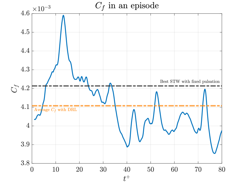
Figure 4: Training of the DRL network - 8 actuations per episode.

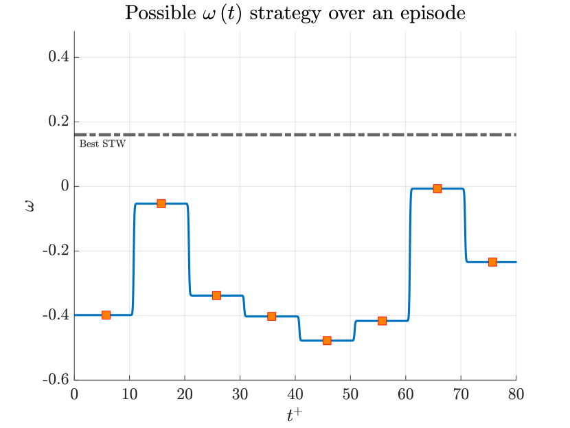
Figure 5: Variation of $\omega$ during one of the episodes with the best $C_{f}$.

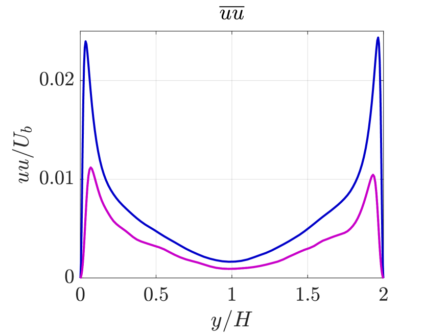
Figure 6: $\overline{uu}$ Reynolds stress reduction between a smooth channel and STW with DRL.

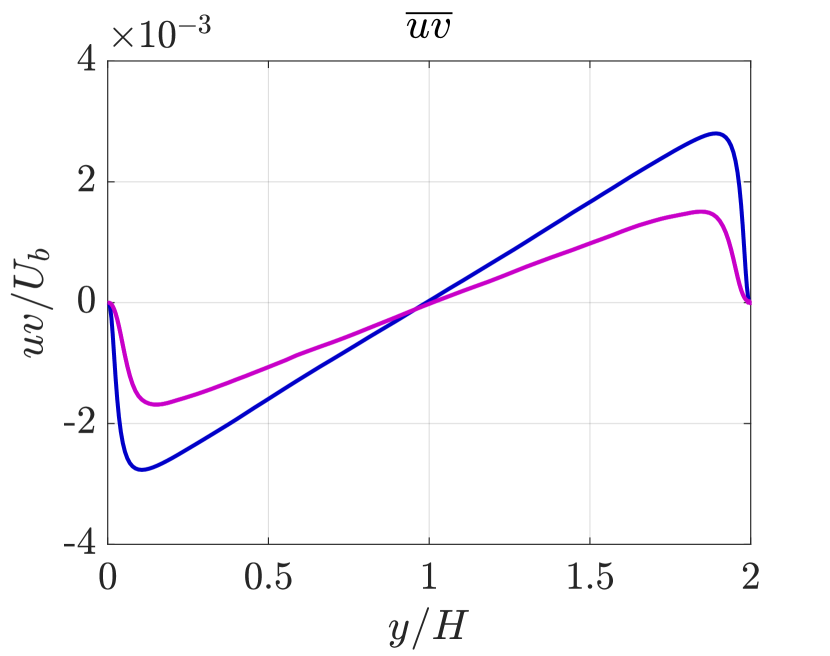
Figure 7: $\overline{uv}$ Reynolds stress reduction between a smooth channel and STW with DRL.

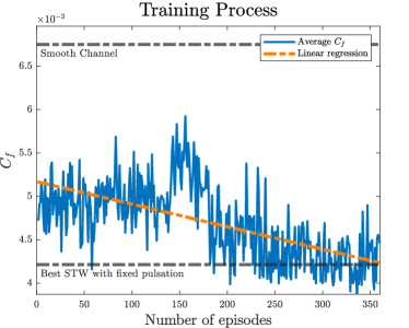
Figure 8: Training process to minimise $C_{f}$. The network starts learning better strategies after 180 episodes, until it reaches a plateau.

The exploration of the effects of this alternative reward was based on a set of modified parameters applied to both the DNS solver and the DRL libraries. Table 2 summarises those modifications. 2. In particular, we have now moved the plane used for data collection to $15^{+}$, while previously it was $\approx 1^{+}$. This location should provide richer information as compared to the previous choice that mainly reflects the state of the laminar sub-layer.

Moreover, $y^{+}=15$ is considered to be an optimal choice for observation planes in DR and flow control feedback [10][2]. However, it should also be mentioned that strategies based on sampling at $y^{+}=1$ remain still appealing due to the possibility of validating with experiments using non intrusive measurements of velocity and stresses at the wall.

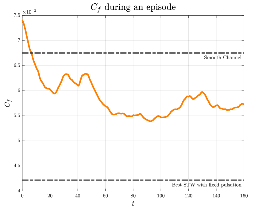
Figure 9: Training of the DRL network - 16 actuations per episode.

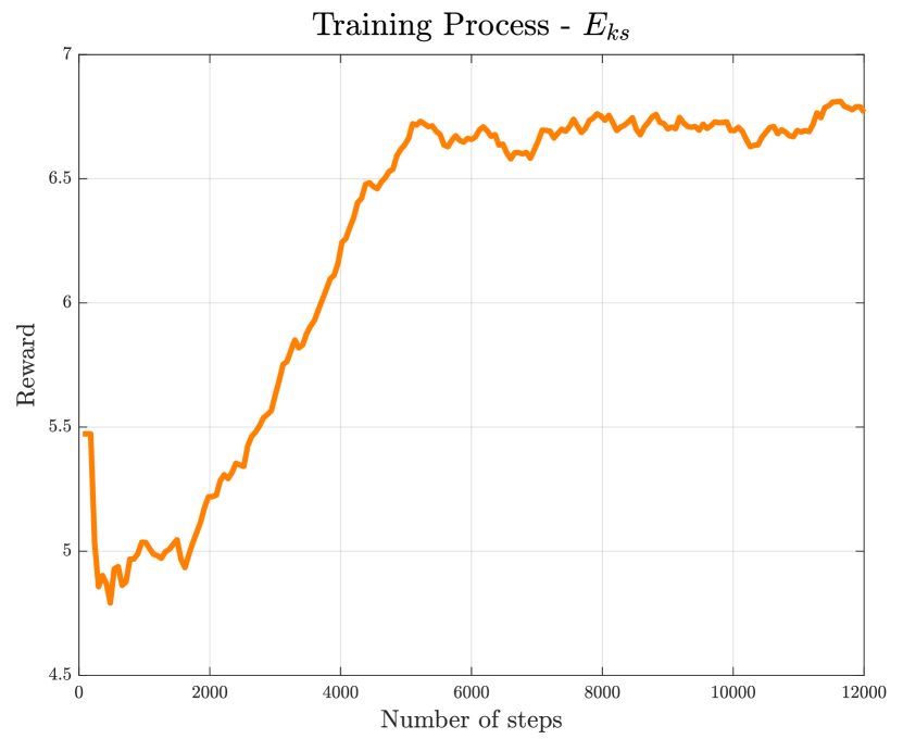
Figure 10: Reward computed as $\tilde{E}_{ks}/\tilde{E}_{k}$ as a function of the step number.

Concerning the actual ML/DNS implementation, it should be mentioned that the training based on StableBaselines3 and CaNS-DNS code is much more complex than the one required for the previous implementation. The main difficulty being related with the management of the communication between the environment and the ML libraries that now takes place using MPI calls and not I/O written on hard disks. Although further improvements are possible, the new implementation offers important advantages in terms of computational efficiency.

Incompressible DNS solver	CaNS
$\left(n_{x},n_{y},n_{z}\right)$	$\left(64,100,96\right)$
$\left(L^{+}_{x},L^{+}_{y},L^{+}_{z}\right)$	$\left(628,200,314\right)$
$Re_{b}$, $Re_{\tau}$ (without STW)	6340, $200$
Simulation time $t^{+}$	160
Actuation time $t^{+}$	10
Cores per simulation	$32+1$
$y^{+}$ for collecting data	15
DRL agent policy	DDPG - PPO
DRL library	StableBaselines3
Python-Fortran interface	MPI (mpi4py)
Input policy	CNN
Network Architecture	variable

Table 2: Parameters used to train the network that promotes topologies with straighter streaks.

Going back to the results obtained when pursuing the maximisation of the streaks energy content, from the time history of $C_{f}$ during an episode, reported in figure 10, two conclusions can be drawn. Firstly, that the we do obtain a significant indirect drag reduction although limited to $20\%$ (against the $45\%$ of Quadrio et al.). Secondly, that the episode duration seems to be sufficient to condition the short-term, transient behaviour of the flow, but not long enough to establish a consistent drag reducing scenario.

It is also noticed that the value of the reward approaches $r=6.7$, as shown in figure 10. For this reward value, the DRL policy is not able to reach values of the ratio $\tilde{E}_{ks}/\tilde{E}_{k}$ greater than $42\%$, with the upper bound not known yet for this kind of control. This limitation may be an indication of the causalities involved in the regeneration cycle and suggest that other integral quantities may be more effective in manipulating the flow behaviour.

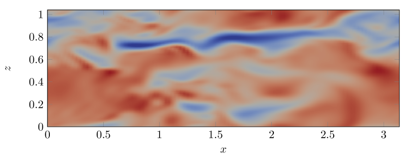
Figure 11: $y^{+}=20$, non-actuated channel
$\tilde{E}_{ks}/\tilde{E}_{k}=33\%$

Figure 12: $y^{+}=20$, $\omega(t)$ STW-DRL control
$\tilde{E}_{ks}/\tilde{E}_{k}=42\%$

Nonetheless, the instantaneous streamwise velocity snapshots extracted on a wall-parallel plane at $y^{+}=20$ for the actuated and non-actuated cases, shown in figures 12 and 12, show that the maximisation of the energy content of the streamwise velocity fluctuations does have an impact on the flow topology. In particular, the actuated case features a smoother behaviour with less entanglement between low and high speed velocity streaks that present a higher, coherent intensity.

4 Discussion and conclusion

The availability of a code featuring a clear, customisable interface enables the proposal of dynamic flow control techniques. Apart from the technological benefit, the same tool can be used to enhance or dampen the effect of various coherent structures embedded in the wall region, opening new avenues in understanding the wall cycle and its manipulation. Here, we presented a case that focused on the fluctuating energy distribution, but other rewards can be envisaged, such as the minimisation of the fourth quadrant events (i.e., sweeps [10]) in the streamwise-wall-normal velocity fluctuations distribution.

Although we have presented only two physical realisations, the primary focus of the present contribution is on the implementation of DRL control techniques within the framework of direct numerical simulations. In the context of this work, several key features and choices need to be highlighted and further explored.

4.1 Actuation duration

One of the most important parameters to set concerns the time period between consecutive $\omega(t)$ adjustments (see 5). Initially, the time interval between actuations $\Delta\tau^{+}$ was set to $10^{+}$. This choice corresponds to a quarter of the standard STW period when $\omega$ is fixed in time in the maximum DR configuration. It was assumed that a possible control law defined by the DRL algorithm would require an actuation update on a similar time scale. Note that $\Delta\tau^{+}=10$ implies up to four actuations on $\omega$ per period of the standard STW, thus giving sufficient relaxation time to the near wall turbulence.

Although we were able to find some interesting results, the choice of a piecewise constant actuation over a certain $\Delta\tau^{+}$ may result in a too restrictive control law that does not allow for the determination of the optimal $\omega(t)$.

The duration of the actuation period can be optimised based on physical considerations. We could start by defining an event $\mathbb{E}$ as a general change in the topology of the structures within the logarithmic layer. The likelihood of this event occurring depends on the conditions at the wall a few time units prior. Ideally, this delay should be slightly shorter, but not too much shorter, than the $\Delta\tau^{+}$ chosen for the actuation period. This would ensure that the action imposed by the STW within the actuation period would have an impact on the close-to-the-wall structures. The agent would also learn faster because the correlation between its actions and the change in the environment would be more direct.

4.2 Hyper-parameter tuning

When tackling increasingly complex optimisation problems, it is important to tune the DRL hyper-parameters. Hyper-parameters are parameters that can be adjusted to modify the learning behaviour and the agent’s features, such as the learning rate and batch size. These hyper-parameters can be adjusted depending on the agent’s policy without altering the DNS environment. However, their impact on training cannot usually be assessed beforehand, necessitating iterative processes to develop and refine a meaningful policy. This process is time-consuming and difficult to estimate in advance. Future studies will include this tuning to avoid sub-optimal policies and ensure convergence toward a satisfactory reward.

4.3 New computational architectures

The numerical simulation of turbulence still predominantly implies the use of CPU-based computer architectures for a series of reasons previously mentioned in the introduction. GPU-based solvers started to appear in the last two decades, with outstanding performances when applied to fully explicit algorithms typical of compressible flow solvers where there is no need for the solution of a pressure Poisson equation. GPU computing for incompressible solvers is more recent although it has been proven to have the potential to exceed the performances of standard CPU-based solvers [14].

Since DRL libraries based on Python are already routinely used on GPUs architecture and the DNS environment is based on CaNS, that offers compiling instructions to work for GPUs architectures, we plan to migrate all the developed software on GPUs or hybrid GPU-CPUs platforms. This should enhance the performances of the overall numerical methodology which will become of paramount importance when using a multi-agent approach in the framework of the previously introduced spanwise strips.

4.4 Conclusion

This study was motivated by the growing opportunities arising from recent algorithms advancements in deep reinforcement learning (DRL) and deep learning. The DRL methodology and related tools are promising candidates for improving flow control techniques by enabling actuations to be governed by policies derived from training a DRL agent. They can also be used to explore the underlying physics of wall turbulence by performing numerical experiments that enhance the presence and the interactions between flow structures. This task may be pursued more efficiently with other types of actuations different from the ones we are currently testing.

Declarations

• Funding: R.V. was supported by ERC Grant No. 2021-CoG-101043998, DEEPCONTROL. The views and opinions expressed are however those of the author(s) only and do not necessarily reflect those of European Union or European Research Council. G.C. would like to acknowledge the support of the EPSRC through their DTP studentships programme, grant number EP/W524608/1.

• Conflict of interest: The authors report no conflict of interest.

• Data access assessment: All the data has been provided in the present article.

References

- \bibcommenthead
- Chorin [1968] Chorin AJ (1968) Numerical Solution of the Navier-Stokes Equations. Mathematics of Computation 22(104):745–762. 10.2307/2004575, 2004575
- Chung and Talha [2011] Chung YM, Talha T (2011) Effectiveness of active flow control for turbulent skin friction drag reduction. Physics of Fluids 23(2):025102. 10.1063/1.3553278
- Cooley and Tukey [1965] Cooley JW, Tukey JW (1965) An Algorithm for the Machine Calculation of Complex Fourier Series. Mathematics of Computation 19(90):297–301. 10.2307/2003354, 2003354
- Costa [2018] Costa P (2018) A FFT-based finite-difference solver for massively-parallel direct numerical simulations of turbulent flows. Computers & Mathematics with Applications 76(8):1853–1862. 10.1016/j.camwa.2018.07.034
- Dalcin and Fang [2021] Dalcin L, Fang YLL (2021) Mpi4py: Status Update After 12 Years of Development. Computing in Science & Engineering 23(4):47–54. 10.1109/MCSE.2021.3083216
- Doohan et al [2021] Doohan P, Willis AP, Hwang Y (2021) Minimal multi-scale dynamics of near-wall turbulence. Journal of Fluid Mechanics 913:A8. 10.1017/jfm.2020.1182
- Font et al [2024] Font B, Alcántara-Ávila F, Rabault J, et al (2024) Active flow control of a turbulent separation bubble through deep reinforcement learning. Journal of Physics: Conference Series 2753(1):012022. 10.1088/1742-6596/2753/1/012022
- Guastoni et al [2021] Guastoni L, Güemes A, Ianiro A, et al (2021) Convolutional-network models to predict wall-bounded turbulence from wall quantities. Journal of Fluid Mechanics 928:A27. 10.1017/jfm.2021.812
- Guastoni et al [2023] Guastoni L, Rabault J, Schlatter P, et al (2023) Deep reinforcement learning for turbulent drag reduction in channel flows. The European Physical Journal E 46(4):27. 10.1140/epje/s10189-023-00285-8
- Hammond et al [1998] Hammond EP, Bewley TR, Moin P (1998) Observed mechanisms for turbulence attenuation and enhancement in opposition-controlled wall-bounded flows. Physics of Fluids 10(9):2421–2423. 10.1063/1.869759
- Harris et al [2020] Harris CR, Millman KJ, van der Walt SJ, et al (2020) Array programming with NumPy. Nature 585(7825):357–362. 10.1038/s41586-020-2649-2
- Jiménez and Moin [1991] Jiménez J, Moin P (1991) The minimal flow unit in near-wall turbulence. Journal of Fluid Mechanics 225:213–240. 10.1017/S0022112091002033
- Jiménez and Pinelli [1999] Jiménez J, Pinelli A (1999) The autonomous cycle of near-wall turbulence. Journal of Fluid Mechanics 389:335–359. 10.1017/S0022112099005066
- Karp et al [2022] Karp M, Massaro D, Jansson N, et al (2022) Large-Scale Direct Numerical Simulations of Turbulence Using GPUs and Modern Fortran. 10.48550/arXiv.2207.07098, 2207.07098
- Kawahara et al [2003] Kawahara G, Jiménez J, Uhlmann M, et al (2003) Linear instability of a corrugated vortex sheet – a model for streak instability. Journal of Fluid Mechanics 483:315–342. 10.1017/S002211200300421X
- LeCun et al [1989] LeCun Y, Boser B, Denker JS, et al (1989) Backpropagation Applied to Handwritten Zip Code Recognition. Neural Computation 1(4):541–551. 10.1162/neco.1989.1.4.541
- Lecun et al [1998] Lecun Y, Bottou L, Bengio Y, et al (1998) Gradient-based learning applied to document recognition. Proceedings of the IEEE 86(11):2278–2324. 10.1109/5.726791
- LeCun et al [2015] LeCun Y, Bengio Y, Hinton G (2015) Deep learning. Nature 521(7553):436–444. 10.1038/nature14539
- Li [2018] Li Y (2018) Deep Reinforcement Learning: An Overview. 10.48550/arXiv.1701.07274, 1701.07274
- Lillicrap et al [2019] Lillicrap TP, Hunt JJ, Pritzel A, et al (2019) Continuous control with deep reinforcement learning. 10.48550/arXiv.1509.02971, 1509.02971
- Monti et al [2019] Monti A, Omidyeganeh M, Pinelli A (2019) Large-eddy simulation of an open-channel flow bounded by a semi-dense rigid filamentous canopy: Scaling and flow structure. Physics of Fluids 31(6):065108. 10.1063/1.5095770
- Monti et al [2020] Monti A, Omidyeganeh M, Eckhardt B, et al (2020) On the genesis of different regimes in canopy flows: A numerical investigation. Journal of Fluid Mechanics 891:A9. 10.1017/jfm.2020.155
- Paszke et al [2019] Paszke A, Gross S, Massa F, et al (2019) PyTorch: An imperative style, high-performance deep learning library. In: Proceedings of the 33rd International Conference on Neural Information Processing Systems. 721, Curran Associates Inc., Red Hook, NY, USA, p 8026–8037
- Quadrio et al [2009] Quadrio M, Ricco P, Viotti C (2009) Streamwise-travelling waves of spanwise wall velocity for turbulent drag reduction. Journal of Fluid Mechanics 627:161–178. 10.1017/S0022112009006077
- Raffin et al [2021] Raffin A, Hill A, Gleave A, et al (2021) Stable-baselines3: Reliable reinforcement learning implementations. Journal of Machine Learning Research 22(268):1–8
- Schulman et al [2017] Schulman J, Wolski F, Dhariwal P, et al (2017) Proximal Policy Optimization Algorithms. 10.48550/arXiv.1707.06347, 1707.06347
- Suárez et al [2024] Suárez P, Álcantara-Ávila F, Rabault J, et al (2024) Flow control of three-dimensional cylinders transitioning to turbulence via multi-agent reinforcement learning. 10.48550/arXiv.2405.17210, 2405.17210
- Vignon et al [2023] Vignon C, Rabault J, Vasanth J, et al (2023) Effective control of two-dimensional Rayleigh–Bénard convection: Invariant multi-agent reinforcement learning is all you need. Physics of Fluids 35(6):065146. 10.1063/5.0153181