Deep Reinforcement Learning: An Overview
Abstract
We give an overview of recent exciting achievements of deep reinforcement learning (RL). We discuss six core elements, six important mechanisms, and twelve applications. We start with background of machine learning, deep learning and reinforcement learning. Next we discuss core RL elements, including value function, in particular, Deep Q-Network (DQN), policy, reward, model and planning, exploration, and knowledge. After that, we discuss important mechanisms for RL, including attention and memory, unsupervised learning, transfer learning, multi-agent RL, hierarchical RL, and learning to learn. Then we discuss various applications of RL, including games, in particular, AlphaGo, robotics, natural language processing, including dialogue systems, machine translation, and text generation, computer vision, business management, finance, healthcare, education, Industry 4.0, smart grid, intelligent transportation systems, and computer systems. We mention topics not reviewed yet, and list a collection of RL resources. After presenting a brief summary, we close with discussions.
This is the first overview about deep reinforcement learning publicly available online. It is comprehensive. Comments and criticisms are welcome. (This particular version is incomplete.)
Please see Deep Reinforcement Learning, https://arxiv.org/abs/1810.06339, for a significant update to this manuscript.
1 Introduction
Reinforcement learning (RL) is about an agent interacting with the environment, learning an optimal policy, by trial and error, for sequential decision making problems in a wide range of fields in both natural and social sciences, and engineering (Sutton and Barto, 1998; 2018; Bertsekas and Tsitsiklis, 1996; Bertsekas, 2012; Szepesvári, 2010; Powell, 2011).
The integration of reinforcement learning and neural networks has a long history (Sutton and Barto, 2018; Bertsekas and Tsitsiklis, 1996; Schmidhuber, 2015). With recent exciting achievements of deep learning (LeCun et al., 2015; Goodfellow et al., 2016), benefiting from big data, powerful computation, new algorithmic techniques, mature software packages and architectures, and strong financial support, we have been witnessing the renaissance of reinforcement learning (Krakovsky, 2016), especially, the combination of deep neural networks and reinforcement learning, i.e., deep reinforcement learning (deep RL).
Deep learning, or deep neural networks, has been prevailing in reinforcement learning in the last several years, in games, robotics, natural language processing, etc. We have been witnessing breakthroughs, like deep Q-network (Mnih et al., 2015) and AlphaGo (Silver et al., 2016a); and novel architectures and applications, like differentiable neural computer (Graves et al., 2016), asynchronous methods (Mnih et al., 2016), dueling network architectures (Wang et al., 2016b), value iteration networks (Tamar et al., 2016), unsupervised reinforcement and auxiliary learning (Jaderberg et al., 2017; Mirowski et al., 2017), neural architecture design (Zoph and Le, 2017), dual learning for machine translation (He et al., 2016a), spoken dialogue systems (Su et al., 2016b), information extraction (Narasimhan et al., 2016), guided policy search (Levine et al., 2016a), and generative adversarial imitation learning (Ho and Ermon, 2016), etc. Creativity would push the frontiers of deep RL further with respect to core elements, mechanisms, and applications.
Why has deep learning been helping reinforcement learning make so many and so enormous achievements? Representation learning with deep learning enables automatic feature engineering and end-to-end learning through gradient descent, so that reliance on domain knowledge is significantly reduced or even removed. Feature engineering used to be done manually and is usually time-consuming, over-specified, and incomplete. Deep, distributed representations exploit the hierarchical composition of factors in data to combat the exponential challenges of the curse of dimensionality. Generality, expressiveness and flexibility of deep neural networks make some tasks easier or possible, e.g., in the breakthroughs and novel architectures and applications discussed above.
Deep learning, as a specific class of machine learning, is not without limitations, e.g., as a black-box lacking interpretability, as an ”alchemy” without clear and sufficient scientific principles to work with, and without human intelligence not able to competing with a baby in some tasks. However, there are lots of works to improve deep learning, machine learning, and AI in general.
Deep learning and reinforcement learning, being selected as one of the MIT Technology Review 10 Breakthrough Technologies in 2013 and 2017 respectively, will play their crucial role in achieving artificial general intelligence. David Silver, the major contributor of AlphaGo (Silver et al., 2016a; 2017), even made a formula: artificial intelligence = reinforcement learning + deep learning (Silver, 2016).
The outline of this overview follows. First we discuss background of machine learning, deep learning and reinforcement learning in Section 2. Next we discuss core RL elements, including value function in Section 3.1, policy in Section 3.2, reward in Section 3.3, model and planning in Section 3.4, exploration in Section 3.5, and knowledge in Section 3.6. Then we discuss important mechanisms for RL, including attention and memory in Section 4.1, unsupervised learning in Section 4.2, transfer learning in Section 4.3, multi-agent RL in Section 4.4, hierarchical RL in Section 4.5, and, learning to learn in Section 4.6. After that, we discuss various RL applications, including games in Section 5.1, robotics in Section 5.2, natural language processing in Section 5.3, computer vision in Section 5.4, business management in Section 5.5, finance in Section 5.6, healthcare in Section 5.7, education in Section 5.8, Industry 4.0 in Section 5.9, smart grid in Section 5.10, intelligent transportation systems in Section 5.11, and computer systems in Section 5.12. We present a list of topics not reviewed yet in Section 6, give a brief summary in Section 8, and close with discussions in Section 9.
In Section 7, we list a collection of RL resources including books, surveys, reports, online courses, tutorials, conferences, journals and workshops, blogs, and open sources. If picking a single RL resource, it is Sutton and Barto’s RL book (Sutton and Barto, 2018), 2nd edition in preparation. It covers RL fundamentals and reflects new progress, e.g., in deep Q-network, AlphaGo, policy gradient methods, as well as in psychology and neuroscience. Deng and Dong (2014) and Goodfellow et al. (2016) are recent deep learning books. Bishop (2011), Hastie et al. (2009), and Murphy (2012) are popular machine learning textbooks; James et al. (2013) gives an introduction to machine learning; Provost and Fawcett (2013) and Kuhn and Johnson (2013) discuss practical issues in machine learning applications; and Simeone (2017) is a brief introduction to machine learning for engineers.
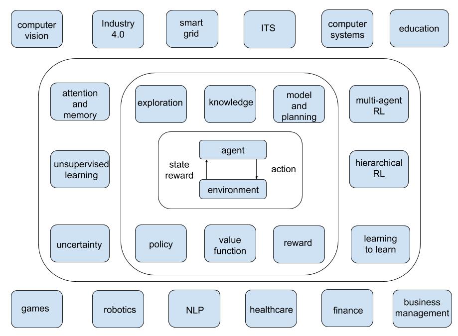
Figure 1 illustrates the conceptual organization of the overview. The agent-environment interaction sits in the center, around which are core elements: value function, policy, reward, model and planning, exploration, and knowledge. Next come important mechanisms: attention and memory, unsupervised learning, transfer learning, multi-agent RL, hierarchical RL, and learning to learn. Then come various applications: games, robotics, NLP (natural language processing), computer vision, business management, finance, healthcare, education, Industry 4.0, smart grid, ITS (intelligent transportation systems), and computer systems.
The main readers of this overview would be those who want to get more familiar with deep reinforcement learning. We endeavour to provide as much relevant information as possible. For reinforcement learning experts, as well as new comers, we hope this overview would be helpful as a reference. In this overview, we mainly focus on contemporary work in recent couple of years, by no means complete, and make slight effort for discussions of historical context, for which the best material to consult is Sutton and Barto (2018).
In this version, we endeavour to provide a wide coverage of fundamental and contemporary RL issues, about core elements, important mechanisms, and applications. In the future, besides further refinements for the width, we will also improve the depth by conducting deeper analysis of the issues involved and the papers discussed. Comments and criticisms are welcome.
2 Background
In this section, we briefly introduce concepts and fundamentals in machine learning, deep learning (Goodfellow et al., 2016) and reinforcement learning (Sutton and Barto, 2018). We do not give detailed background introduction for machine learning and deep learning. Instead, we recommend the following recent Nature/Science survey papers: Jordan and Mitchell (2015) for machine learning, and LeCun et al. (2015) for deep learning. We cover some RL basics. However, we recommend the textbook, Sutton and Barto (2018), and the recent Nature survey paper, Littman (2015), for reinforcement learning. We also collect relevant resources in Section 7.
2.1 Machine Learning
Machine learning is about learning from data and making predictions and/or decisions.
Usually we categorize machine learning as supervised, unsupervised, and reinforcement learning.111Is reinforcement learning part of machine learning, or more than it, and somewhere close to artificial intelligence? We raise this question without elaboration. In supervised learning, there are labeled data; in unsupervised learning, there are no labeled data; and in reinforcement learning, there are evaluative feedbacks, but no supervised signals. Classification and regression are two types of supervised learning problems, with categorical and numerical outputs respectively.
Unsupervised learning attempts to extract information from data without labels, e.g., clustering and density estimation. Representation learning is a classical type of unsupervised learning. However, training feedforward networks or convolutional neural networks with supervised learning is a kind of representation learning. Representation learning finds a representation to preserve as much information about the original data as possible, at the same time, to keep the representation simpler or more accessible than the original data, with low-dimensional, sparse, and independent representations.
Deep learning, or deep neural networks, is a particular machine learning scheme, usually for supervised or unsupervised learning, and can be integrated with reinforcement learning, usually as a function approximator. Supervised and unsupervised learning are usually one-shot, myopic, considering instant reward; while reinforcement learning is sequential, far-sighted, considering long-term accumulative reward.
Machine learning is based on probability theory and statistics (Hastie et al., 2009) and optimization (Boyd and Vandenberghe, 2004), is the basis for big data, data science (Blei and Smyth, 2017; Provost and Fawcett, 2013), predictive modeling (Kuhn and Johnson, 2013), data mining, information retrieval (Manning et al., 2008), etc, and becomes a critical ingredient for computer vision, natural language processing, robotics, etc. Reinforcement learning is kin to optimal control (Bertsekas, 2012), and operations research and management (Powell, 2011), and is also related to psychology and neuroscience (Sutton and Barto, 2018). Machine learning is a subset of artificial intelligence (AI), and is evolving to be critical for all fields of AI.
A machine learning algorithm is composed of a dataset, a cost/loss function, an optimization procedure, and a model (Goodfellow et al., 2016). A dataset is divided into non-overlapping training, validation, and testing subsets. A cost/loss function measures the model performance, e.g., with respect to accuracy, like mean square error in regression and classification error rate. Training error measures the error on the training data, minimizing which is an optimization problem. Generalization error, or test error, measures the error on new input data, which differentiates machine learning from optimization. A machine learning algorithm tries to make the training error, and the gap between training error and testing error small. A model is under-fitting if it can not achieve a low training error; a model is over-fitting if the gap between training error and test error is large.
A model’s capacity measures the range of functions it can fit. VC dimension measures the capacity of a binary classifier. Occam’s Razor states that, with the same expressiveness, simple models are preferred. Training error and generalization error versus model capacity usually form a U-shape relationship. We find the optimal capacity to achieve low training error and small gap between training error and generalization error. Bias measures the expected deviation of the estimator from the true value; while variance measures the deviation of the estimator from the expected value, or variance of the estimator. As model capacity increases, bias tends to decrease, while variance tends to increase, yielding another U-shape relationship between generalization error versus model capacity. We try to find the optimal capacity point, of which under-fitting occurs on the left and over-fitting occurs on the right. Regularization add a penalty term to the cost function, to reduce the generalization error, but not training error. No free lunch theorem states that there is no universally best model, or best regularizor. An implication is that deep learning may not be the best model for some problems. There are model parameters, and hyperparameters for model capacity and regularization. Cross-validation is used to tune hyperparameters, to strike a balance between bias and variance, and to select the optimal model.
Maximum likelihood estimation (MLE) is a common approach to derive good estimation of parameters. For issues like numerical underflow, the product in MLE is converted to summation to obtain negative log-likelihood (NLL). MLE is equivalent to minimizing KL divergence, the dissimilarity between the empirical distribution defined by the training data and the model distribution. Minimizing KL divergence between two distributions corresponds to minimizing the cross-entropy between the distributions. In short, maximization of likelihood becomes minimization of the negative log-likelihood (NLL), or equivalently, minimization of cross entropy.
Gradient descent is a common approach to solve optimization problems. Stochastic gradient descent extends gradient descent by working with a single sample each time, and usually with minibatches.
Importance sampling is a technique to estimate properties of a particular distribution, by samples from a different distribution, to lower the variance of the estimation, or when sampling from the distribution of interest is difficult.
Frequentist statistics estimates a single value, and characterizes variance by confidence interval; Bayesian statistics considers the distribution of an estimate when making predictions and decisions.
generative vs discriminative
2.2 Deep Learning
Deep learning is in contrast to ”shallow” learning. For many machine learning algorithms, e.g., linear regression, logistic regression, support vector machines (SVMs), decision trees, and boosting, we have input layer and output layer, and the inputs may be transformed with manual feature engineering before training. In deep learning, between input and output layers, we have one or more hidden layers. At each layer except input layer, we compute the input to each unit, as the weighted sum of units from the previous layer; then we usually use nonlinear transformation, or activation function, such as logistic, tanh, or more popular recently, rectified linear unit (ReLU), to apply to the input of a unit, to obtain a new representation of the input from previous layer. We have weights on links between units from layer to layer. After computations flow forward from input to output, at output layer and each hidden layer, we can compute error derivatives backward, and backpropagate gradients towards the input layer, so that weights can be updated to optimize some loss function.
A feedforward deep neural network or multilayer perceptron (MLP) is to map a set of input values to output values with a mathematical function formed by composing many simpler functions at each layer. A convolutional neural network (CNN) is a feedforward deep neural network, with convolutional layers, pooling layers and fully connected layers. CNNs are designed to process data with multiple arrays, e.g., colour image, language, audio spectrogram, and video, benefit from the properties of such signals: local connections, shared weights, pooling and the use of many layers, and are inspired by simple cells and complex cells in visual neuroscience (LeCun et al., 2015). ResNets (He et al., 2016d) are designed to ease the training of very deep neural networks by adding shortcut connections to learn residual functions with reference to the layer inputs. A recurrent neural network (RNN) is often used to process sequential inputs like speech and language, element by element, with hidden units to store history of past elements. A RNN can be seen as a multilayer neural network with all layers sharing the same weights, when being unfolded in time of forward computation. It is hard for RNN to store information for very long time and the gradient may vanish. Long short term memory networks (LSTM) (Hochreiter and Schmidhuber, 1997) and gated recurrent unit (GRU) (Chung et al., 2014) were proposed to address such issues, with gating mechanisms to manipulate information through recurrent cells. Gradient backpropagation or its variants can be used for training all deep neural networks mentioned above.
Dropout (Srivastava et al., 2014) is a regularization strategy to train an ensemble of sub-networks by removing non-output units randomly from the original network. Batch normalization (Ioffe and Szegedy, 2015) performs the normalization for each training mini-batch, to accelerate training by reducing internal covariate shift, i.e., the change of parameters of previous layers will change each layer’s inputs distribution.
Deep neural networks learn representations automatically from raw inputs to recover the compositional hierarchies in many natural signals, i.e., higher-level features are composed of lower-level ones, e.g., in images, the hierarch of objects, parts, motifs, and local combinations of edges. Distributed representation is a central idea in deep learning, which implies that many features may represent each input, and each feature may represent many inputs. The exponential advantages of deep, distributed representations combat the exponential challenges of the curse of dimensionality. The notion of end-to-end training refers to that a learning model uses raw inputs without manual feature engineering to generate outputs, e.g., AlexNet (Krizhevsky et al., 2012) with raw pixels for image classification, Seq2Seq (Sutskever et al., 2014) with raw sentences for machine translation, and DQN (Mnih et al., 2015) with raw pixels and score to play games.
2.3 Reinforcement Learning
We provide background of reinforcement learning briefly in this section. After setting up the RL problem, we discuss value function, temporal difference learning, function approximation, policy optimization, deep RL, RL parlance, and close this section with a brief summary. To have a good understanding of deep reinforcement learning, it is essential to have a good understanding of reinforcement learning first.
2.3.1 Problem Setup
A RL agent interacts with an environment over time. At each time step , the agent receives a state in a state space and selects an action from an action space , following a policy , which is the agent’s behavior, i.e., a mapping from state to actions , receives a scalar reward , and transitions to the next state , according to the environment dynamics, or model, for reward function and state transition probability respectively. In an episodic problem, this process continues until the agent reaches a terminal state and then it restarts. The return is the discounted, accumulated reward with the discount factor . The agent aims to maximize the expectation of such long term return from each state. The problem is set up in discrete state and action spaces. It is not hard to extend it to continuous spaces.
2.3.2 Exploration vs Exploitation
multi-arm bandit
various exploration techniques
2.3.3 Value Function
A value function is a prediction of the expected, accumulative, discounted, future reward, measuring how good each state, or state-action pair, is. The state value is the expected return for following policy from state . decomposes into the Bellman equation: . An optimal state value is the maximum state value achievable by any policy for state . decomposes into the Bellman equation: . The action value is the expected return for selecting action in state and then following policy . decomposes into the Bellman equation: . An optimal action value function is the maximum action value achievable by any policy for state and action . decomposes into the Bellman equation: . We denote an optimal policy by .
2.3.4 Dynamic Programming
2.3.5 Temporal Difference Learning
When a RL problem satisfies the Markov property, i.e., the future depends only on the current state and action, but not on the past, it is formulated as a Markov Decision Process (MDP), defined by the 5-tuple . When the system model is available, we use dynamic programming methods: policy evaluation to calculate value/action value function for a policy, value iteration and policy iteration for finding an optimal policy. When there is no model, we resort to RL methods. RL methods also work when the model is available. Additionally, a RL environment can be a multi-armed bandit, an MDP, a POMDP, a game, etc.
Temporal difference (TD) learning is central in RL. TD learning is usually refer to the learning methods for value function evaluation in Sutton (1988). SARSA (Sutton and Barto, 2018) and Q-learning (Watkins and Dayan, 1992) are also regarded as temporal difference learning.
TD learning (Sutton, 1988) learns value function directly from experience with TD error, with bootstrapping, in a model-free, online, and fully incremental way. TD learning is a prediction problem. The update rule is , where is a learning rate, and is called TD error. Algorithm 1 presents the pseudo code for tabular TD learning. Precisely, it is tabular TD(0) learning, where ”0” indicates it is based on one-step return.
Bootstrapping, like the TD update rule, estimates state or action value based on subsequent estimates, is common in RL, like TD learning, Q learning, and actor-critic. Bootstrapping methods are usually faster to learn, and enable learning to be online and continual. Bootstrapping methods are not instances of true gradient decent, since the target depends on the weights to be estimated. The concept of semi-gradient descent is then introduced (Sutton and Barto, 2018).
SARSA, representing state, action, reward, (next) state, (next) action, is an on-policy control method to find the optimal policy, with the update rule, . Algorithm 2 presents the pseudo code for tabular SARSA, precisely tabular SARSA(0).
Q-learning is an off-policy control method to find the optimal policy. Q-learning learns action value function, with the update rule, . Q learning refines the policy greedily with respect to action values by the max operator. Algorithm 3 presents the pseudo code for Q learning, precisely, tabular Q(0) learning.
TD-learning, Q-learning and SARSA converge under certain conditions. From an optimal action value function, we can derive an optimal policy.
2.3.6 Multi-step Bootstrapping
The above algorithms are referred to as TD(0) and Q(0), learning with one-step return. We have TD learning and Q learning variants and Monte-Carlo approach with multi-step return in the forward view. The eligibility trace from the backward view provides an online, incremental implementation, resulting in TD() and Q() algorithms, where . TD(1) is the same as the Monte Carlo approach.
Eligibility trace is a short-term memory, usually lasting within an episode, assists the learning process, by affecting the weight vector. The weight vector is a long-term memory, lasting the whole duration of the system, determines the estimated value. Eligibility trace helps with the issues of long-delayed rewards and non-Markov tasks (Sutton and Barto, 2018).
TD() unifies one-step TD prediction, TD(0), with Monte Carlo methods, TD(1), using eligibility traces and the decay parameter , for prediction algorithms. De Asis et al. (2018) made unification for multi-step TD control algorithms.
2.3.7 Function Approximation
We discuss the tabular cases above, where a value function or a policy is stored in a tabular form. Function approximation is a way for generalization when the state and/or action spaces are large or continuous. Function approximation aims to generalize from examples of a function to construct an approximate of the entire function; it is usually a concept in supervised learning, studied in the fields of machine learning, patten recognition, and statistical curve fitting; function approximation in reinforcement learning usually treats each backup as a training example, and encounters new issues like nonstationarity, bootstrapping, and delayed targets (Sutton and Barto, 2018). Linear function approximation is a popular choice, partially due to its desirable theoretical properties, esp. before the work of Deep Q-Network (Mnih et al., 2015). However, the integration of reinforcement learning and neural networks dated back a long time ago (Sutton and Barto, 2018; Bertsekas and Tsitsiklis, 1996; Schmidhuber, 2015).
Algorithm 4 presents the pseudo code for TD(0) with function approximation. is the approximate value function, is the value function weight vector, is the gradient of the approximate value function with respect to the weight vector, and the weight vector is updated following the update rule, .
When combining off-policy, function approximation, and bootstrapping, instability and divergence may occur (Tsitsiklis and Van Roy, 1997), which is called the deadly triad issue (Sutton and Barto, 2018). All these three elements are necessary: function approximation for scalability and generalization, bootstrapping for computational and data efficiency, and off-policy learning for freeing behaviour policy from target policy. What is the root cause for the instability? Learning or sampling are not, since dynamic programming suffers from divergence with function approximation; exploration, greedification, or control are not, since prediction alone can diverge; local minima or complex non-linear function approximation are not, since linear function approximation can produce instability (Sutton, 2016). It is unclear what is the root cause for instability – each single factor mentioned above is not – there are still many open problems in off-policy learning (Sutton and Barto, 2018).
Table 1 presents various algorithms that tackle various issues (Sutton, 2016). Deep RL algorithms like Deep Q-Network (Mnih et al., 2015) and A3C (Mnih et al., 2016) are not presented here, since they do not have theoretical guarantee, although they achieve stunning performance empirically.
Before explaining Table 1, we introduce some background definitions. Recall that Bellman equation for value function is . Bellman operator is defined as . TD fix point is then . Bellman error for the function approximation case is then , the right side of Bellman equation with function approximation minus the left side. It can be written as . Bellman error is the expectation of the TD error.
ADP algorithms refer to dynamic programming algorithms like policy evaluation, policy iteration, and value iteration, with function approximation. Least square temporal difference (LSTD) (Bradtke and Barto, 1996) computes TD fix-point directly in batch mode. LSTD is data efficient, yet with squared time complexity. LSPE (Nedić and Bertsekas, 2003) extended LSTD. Fitted-Q algorithms (Ernst et al., 2005; Riedmiller, 2005) learn action values in batch mode. Residual gradient algorithms (Baird, 1995) minimize Bellman error. Gradient-TD (Sutton et al., 2009a; b; Mahmood et al., 2014) methods are true gradient algorithms, perform SGD in the projected Bellman error (PBE), converge robustly under off-policy training and non-linear function approximation. Emphatic-TD (Sutton et al., 2016) emphasizes some updates and de-emphasizes others by reweighting, improving computational efficiency, yet being a semi-gradient method. See Sutton and Barto (2018) for more details. Du et al. (2017) proposed variance reduction techniques for policy evaluation to achieve fast convergence. White and White (2016) performed empirical comparisons of linear TD methods, and made suggestions about their practical use.
| algorithm | ||||||||
|---|---|---|---|---|---|---|---|---|
| TD() SARSA() | ADP | LSTD() LSPE() | Fitted-Q | Residual Gradient | GTD() GQ() | |||
| linear computation | ||||||||
| issue | nonlinear convergent | |||||||
| off-policy convergent | ||||||||
| model-free, online | ||||||||
| converges to PBE = 0 | ||||||||
2.3.8 Policy Optimization
In contrast to value-based methods like TD learning and Q-learning, policy-based methods optimize the policy (with function approximation) directly, and update the parameters by gradient ascent on . REINFORCE (Williams, 1992) is a policy gradient method, updating in the direction of . Usually a baseline is subtracted from the return to reduce the variance of gradient estimate, yet keeping its unbiasedness, to yield the gradient direction . Using as the baseline , we have the advantage function , since is an estimate of . Algorithm 5 presents the pseudo code for REINFORCE algorithm in the episodic case.
In actor-critic algorithms, the critic updates action-value function parameters, and the actor updates policy parameters, in the direction suggested by the critic. Algorithm 6 presents the pseudo code for one-step actor-critic algorithm in the episodic case.
Policy iteration alternates between policy evaluation and policy improvement, to generate a sequence of improving policies. In policy evaluation, the value function of the current policy is estimated from the outcomes of sampled trajectories. In policy improvement, the current value function is used to generate a better policy, e.g., by selecting actions greedily with respect to the value function.
2.3.9 Deep Reinforcement Learning
We obtain deep reinforcement learning (deep RL) methods when we use deep neural networks to approximate any of the following components of reinforcement learning: value function, or , policy , and model (state transition function and reward function). Here, the parameters are the weights in deep neural networks. When we use ”shallow” models, like linear function, decision trees, tile coding and so on as the function approximator, we obtain ”shallow” RL, and the parameters are the weight parameters in these models. Note, a shallow model, e.g., decision trees, may be non-linear. The distinct difference between deep RL and ”shallow” RL is what function approximator is used. This is similar to the difference between deep learning and ”shallow” machine learning. We usually utilize stochastic gradient descent to update weight parameters in deep RL. When off-policy, function approximation, in particular, non-linear function approximation, and bootstrapping are combined together, instability and divergence may occur (Tsitsiklis and Van Roy, 1997). However, recent work like Deep Q-Network (Mnih et al., 2015) and AlphaGo (Silver et al., 2016a) stabilized the learning and achieved outstanding results.
2.3.10 RL Parlance
We explain some terms in RL parlance.
The prediction problem, or policy evaluation, is to compute the state or action value function for a policy. The control problem is to find the optimal policy. Planning constructs a value function or a policy with a model.
On-policy methods evaluate or improve the behavioural policy, e.g., SARSA fits the action-value function to the current policy, i.e., SARSA evaluates the policy based on samples from the same policy, then refines the policy greedily with respect to action values. In off-policy methods, an agent learns an optimal value function/policy, maybe following an unrelated behavioural policy, e.g., Q-learning attempts to find action values for the optimal policy directly, not necessarily fitting to the policy generating the data, i.e., the policy Q-learning obtains is usually different from the policy that generates the samples. The notion of on-policy and off-policy can be understood as same-policy and different-policy.
The exploration-exploitation dilemma is about the agent needs to exploit the currently best action to maximize rewards greedily, yet it has to explore the environment to find better actions, when the policy is not optimal yet, or the system is non-stationary.
In model-free methods, the agent learns with trail-and-error from experience explicitly; the model (state transition function) is not known or learned from experience. RL methods that use models are model-based methods.
In online mode, training algorithms are executed on data acquired in sequence. In offline mode, or batch mode, models are trained on the entire data set.
With bootstrapping, an estimate of state or action value is updated from subsequent estimates.
2.3.11 Brief Summary
A RL problem is formulated as an MDP when the observation about the environment satisfies the Markov property. An MDP is defined by the 5-tuple . A central concept in RL is value function. Bellman equations are cornerstone for developing RL algorithms. Temporal difference learning algorithms are fundamental for evaluating/predicting value functions. Control algorithms find optimal policies. Reinforcement learning algorithms may be based on value function and/or policy, model-free or model-based, on-policy or off-policy, with function approximation or not, with sample backups (TD and Monte Carlo) or full backups (dynamic programming and exhaustive search), and about the depth of backups, either one-step return (TD(0) and dynamic programming) or multi-step return (TD(), Monte Carlo, and exhaustive search). When combining off-policy, function approximation, and bootstrapping, we face instability and divergence (Tsitsiklis and Van Roy, 1997), the deadly triad issue (Sutton and Barto, 2018). Theoretical guarantee has been established for linear function approximation, e.g., Gradient-TD (Sutton et al., 2009a; b; Mahmood et al., 2014), Emphatic-TD (Sutton et al., 2016) and Du et al. (2017). With non-linear function approximation, in particular deep learning, algorithms like Deep Q-Network (Mnih et al., 2015) and AlphaGo (Silver et al., 2016a; 2017) stabilized the learning and achieved stunning results, which is the focus of this overview.
3 Core Elements
A RL agent executes a sequence of actions and observe states and rewards, with major components of value function, policy and model. A RL problem may be formulated as a prediction, control or planning problem, and solution methods may be model-free or model-based, with value function and/or policy. Exploration-exploitation is a fundamental tradeoff in RL. Knowledge would be critical for RL. In this section, we discuss core RL elements: value function in Section 3.1, policy in Section 3.2, reward in Section 3.3, model and planning in Section 3.4, exploration in Section 3.5, and knowledge in Section 3.6.
3.1 Value Function
Value function is a fundamental concept in reinforcement learning, and temporal difference (TD) learning (Sutton, 1988) and its extension, Q-learning (Watkins and Dayan, 1992), are classical algorithms for learning state and action value functions respectively. In the following, we focus on Deep Q-Network (Mnih et al., 2015), a recent breakthrough, and its extensions.
3.1.1 Deep Q-Network (DQN) And Extensions
Mnih et al. (2015) introduced Deep Q-Network (DQN) and ignited the field of deep RL. We present DQN pseudo code in Algorithm 7.
Before DQN, it is well known that RL is unstable or even divergent when action value function is approximated with a nonlinear function like neural networks. DQN made several important contributions: 1) stabilize the training of action value function approximation with deep neural networks (CNN) using experience replay (Lin, 1992) and target network; 2) designing an end-to-end RL approach, with only the pixels and the game score as inputs, so that only minimal domain knowledge is required; 3) training a flexible network with the same algorithm, network architecture and hyperparameters to perform well on many different tasks, i.e., 49 Atari games (Bellemare et al., 2013), and outperforming previous algorithms and performing comparably to a human professional tester.
See Chapter 16 in Sutton and Barto (2018) for a detailed and intuitive description of Deep Q-Network. See Deepmind’s description of DQN at https://deepmind.com/research/dqn/.
Double DQN
van Hasselt et al. (2016a) proposed Double DQN (D-DQN) to tackle the over-estimate problem in Q-learning. In standard Q-learning, as well as in DQN, the parameters are updated as follows:
where
so that the max operator uses the same values to both select and evaluate an action. As a consequence, it is more likely to select over-estimated values, and results in over-optimistic value estimates. van Hasselt et al. (2016a) proposed to evaluate the greedy policy according to the online network, but to use the target network to estimate its value. This can be achieved with a minor change to the DQN algorithm, replacing with
where is the parameter for online network and is the parameter for target network. For reference, can be written as
D-DQN found better policies than DQN on Atari games.
Prioritized Experience Replay
In DQN, experience transitions are uniformly sampled from the replay memory, regardless of the significance of experiences. Schaul et al. (2016) proposed to prioritize experience replay, so that important experience transitions can be replayed more frequently, to learn more efficiently. The importance of experience transitions are measured by TD errors. The authors designed a stochastic prioritization based on the TD errors, using importance sampling to avoid the bias in the update distribution. The authors used prioritized experience replay in DQN and D-DQN, and improved their performance on Atari games.
Dueling Architecture
Wang et al. (2016b) proposed the dueling network architecture to estimate state value function and associated advantage function , and then combine them to estimate action value function , to converge faster than Q-learning. In DQN, a CNN layer is followed by a fully connected (FC) layer. In dueling architecture, a CNN layer is followed by two streams of FC layers, to estimate value function and advantage function separately; then the two streams are combined to estimate action value function. Usually we use the following to combine and to obtain ,
where and are parameters of the two streams of FC layers. Wang et al. (2016b) proposed to replace max operator with average as the following for better stability,
Dueling architecture implemented with D-DQN and prioritized experience replay improved previous work, DQN and D-DQN with prioritized experience replay, on Atari games.
Distributional Value Function
Bellemare et al. (2017)
Rainbow
Hessel et al. (2018)
More DQN Extensions
DQN has been receiving much attention. We list several extensions/improvements here.
-
•
Anschel et al. (2017) proposed to reduce variability and instability by an average of previous Q-values estimates.
-
•
He et al. (2017) proposed to accelerate DQN by optimality tightening, a constrained optimization approach, to propagate reward faster, and to improve accuracy over DQN.
-
•
Liang et al. (2016) attempted to understand the success of DQN and reproduced results with shallow RL.
- •
-
•
Oh et al. (2015) proposed spatio-temporal video prediction conditioned on actions and previous video frames with deep neural networks in Atari games.
-
•
Osband et al. (2016) designed better exploration strategy to improve DQN.
- •
3.2 Policy
A policy maps state to action, and policy optimization is to find an optimal mapping. As in Peters and Neumann (2015), the spectrum from direct policy search to value-based RL includes: evolutionary strategies, CMA-ES (covariance matrix adaptation evolution strategy), episodic REPS (relative entropy policy search), policy gradients, PILCO (probabilistic inference for learning control) (Deisenroth and Rasmussen, 2011), model-based REPS, policy search by trajectory optimization, actor critic, natural actor critic, eNAC (episodic natural actor critic), advantage weighted regression, conservative policy iteration, LSPI (least square policy iteration) (Lagoudakis and Parr, 2003), Q-learning, and fitted Q, as well as important extensions, contextual policy search, and hierarchical policy search.
We discuss actor-critic (Mnih et al., 2016). Then we discuss policy gradient, including deterministic policy gradient (Silver et al., 2014; Lillicrap et al., 2016), trust region policy optimization (Schulman et al., 2015), and, benchmark results (Duan et al., 2016). Next we discuss the combination of policy gradient and off-policy RL (O’Donoghue et al., 2017; Nachum et al., 2017; Gu et al., 2017).
See Retrace algorithm (Munos et al., 2016), a safe and efficient return-based off-policy control algorithm, and its actor-critic extension, Reactor (Gruslys et al., 2017), for Retrace-actor. See distributed proximal policy optimization (Heess et al., 2017). McAllister and Rasmussen (2017) extended PILCO to POMDPs.
3.2.1 Actor-Critic
An actor-critic algorithm learns both a policy and a state-value function, and the value function is used for bootstrapping, i.e., updating a state from subsequent estimates, to reduce variance and accelerate learning (Sutton and Barto, 2018). In the following, we focus on asynchronous advantage actor-critic (A3C) (Mnih et al., 2016). Mnih et al. (2016) also discussed asynchronous one-step SARSA, one-step Q-learning and n-step Q-learning.
In A3C, parallel actors employ different exploration policies to stabilize training, so that experience replay is not utilized. Different from most deep learning algorithms, asynchronous methods can run on a single multi-core CPU. For Atari games, A3C ran much faster yet performed better than or comparably with DQN, Gorila (Nair et al., 2015), D-DQN, Dueling D-DQN, and Prioritized D-DQN. A3C also succeeded on continuous motor control problems: TORCS car racing games and MujoCo physics manipulation and locomotion, and Labyrinth, a navigating task in random 3D mazes using visual inputs, in which an agent will face a new maze in each new episode, so that it needs to learn a general strategy to explore random mazes.
We present pseudo code for asynchronous advantage actor-critic for each actor-learner thread in Algorithm 8. A3C maintains a policy and an estimate of the value function , being updated with -step returns in the forward view, after every actions or reaching a terminal state, similar to using minibatches. The gradient update can be seen as , where is an estimate of the advantage function, with upbounded by .
Wang et al. (2017b) proposed a stable and sample efficient actor-critic deep RL model using experience replay, with truncated importance sampling, stochastic dueling network (Wang et al., 2016b) as discussed in Section 3.1, and trust region policy optimization (Schulman et al., 2015) as discussed in Section 3.2. Babaeizadeh et al. (2017) proposed a hybrid CPU/GPU implementation of A3C.
3.2.2 Policy Gradient
Deterministic Policy Gradient
Policies are usually stochastic. However, Silver et al. (2014) and Lillicrap et al. (2016) proposed deterministic policy gradient (DPG) for efficient estimation of policy gradients.
Silver et al. (2014) introduced the deterministic policy gradient (DPG) algorithm for RL problems with continuous action spaces. The deterministic policy gradient is the expected gradient of the action-value function, which integrates over the state space; whereas in the stochastic case, the policy gradient integrates over both state and action spaces. Consequently, the deterministic policy gradient can be estimated more efficiently than the stochastic policy gradient. The authors introduced an off-policy actor-critic algorithm to learn a deterministic target policy from an exploratory behaviour policy, and to ensure unbiased policy gradient with the compatible function approximation for deterministic policy gradients. Empirical results showed its superior to stochastic policy gradients, in particular in high dimensional tasks, on several problems: a high-dimensional bandit; standard benchmark RL tasks of mountain car and pendulum and 2D puddle world with low dimensional action spaces; and controlling an octopus arm with a high-dimensional action space. The experiments were conducted with tile-coding and linear function approximators.
Lillicrap et al. (2016) proposed an actor-critic, model-free, deep deterministic policy gradient (DDPG) algorithm in continuous action spaces, by extending DQN (Mnih et al., 2015) and DPG (Silver et al., 2014). With actor-critic as in DPG, DDPG avoids the optimization of action at every time step to obtain a greedy policy as in Q-learning, which will make it infeasible in complex action spaces with large, unconstrained function approximators like deep neural networks. To make the learning stable and robust, similar to DQN, DDPQ deploys experience replay and an idea similar to target network, ”soft” target, which, rather than copying the weights directly as in DQN, updates the soft target network weights slowly to track the learned networks weights : , with . The authors adapted batch normalization to handle the issue that the different components of the observation with different physical units. As an off-policy algorithm, DDPG learns an actor policy from experiences from an exploration policy by adding noise sampled from a noise process to the actor policy. More than 20 simulated physics tasks of varying difficulty in the MuJoCo environment were solved with the same learning algorithm, network architecture and hyper-parameters, and obtained policies with performance competitive with those found by a planning algorithm with full access to the underlying physical model and its derivatives. DDPG can solve problems with 20 times fewer steps of experience than DQN, although it still needs a large number of training episodes to find solutions, as in most model-free RL methods. It is end-to-end, with raw pixels as input. DDPQ paper also contains links to videos for illustration.
Hausknecht and Stone (2016) considers parameterization of action space.
Trust Region Policy Optimization
Schulman et al. (2015) introduced an iterative procedure to monotonically improve policies theoretically, guaranteed by optimizing a surrogate objective function. The authors then proposed a practical algorithm, Trust Region Policy Optimization (TRPO), by making several approximations, including, introducing a trust region constraint, defined by the KL divergence between the new policy and the old policy, so that at every point in the state space, the KL divergence is bounded; approximating the trust region constraint by the average KL divergence constraint; replacing the expectations and Q value in the optimization problem by sample estimates, with two variants: in the single path approach, individual trajectories are sampled; in the vine approach, a rollout set is constructed and multiple actions are performed from each state in the rollout set; and, solving the constrained optimization problem approximately to update the policy’s parameter vector. The authors also unified policy iteration and policy gradient with analysis, and showed that policy iteration, policy gradient, and natural policy gradient (Kakade, 2002) are special cases of TRPO. In the experiments, TRPO methods performed well on simulated robotic tasks of swimming, hopping, and walking, as well as playing Atari games in an end-to-end manner directly from raw images.
Wu et al. (2017) proposed scalable TRPO with Kronecker-factored approximation to the curvature.
https://blog.openai.com/openai-baselines-ppo/
Benchmark Results
Duan et al. (2016) presented a benchmark for continuous control tasks, including classic tasks like cart-pole, tasks with very large state and action spaces such as 3D humanoid locomotion and tasks with partial observations, and tasks with hierarchical structure, implemented various algorithms, including batch algorithms: REINFORCE, Truncated Natural Policy Gradient (TNPG), Reward-Weighted Regression (RWR), Relative Entropy Policy Search (REPS), Trust Region Policy Optimization (TRPO), Cross Entropy Method (CEM), Covariance Matrix Adaption Evolution Strategy (CMA-ES); online algorithms: Deep Deterministic Policy Gradient (DDPG); and recurrent variants of batch algorithms. The open source is available at: https://github.com/rllab/rllab.
Duan et al. (2016) compared various algorithms, and showed that DDPG, TRPO, and Truncated Natural Policy Gradient (TNPG) (Schulman et al., 2015) are effective in training deep neural network policies, yet better algorithms are called for hierarchical tasks.
Islam et al. (2017)
Tassa et al. (2018)
3.2.3 Combining Policy Gradient with Off-Policy RL
O’Donoghue et al. (2017) proposed to combine policy gradient with off-policy Q-learning (PGQ), to benefit from experience replay. Usually actor-critic methods are on-policy. The authors also showed that action value fitting techniques and actor-critic methods are equivalent, and interpreted regularized policy gradient techniques as advantage function learning algorithms. Empirically, the authors showed that PGQ outperformed DQN and A3C on Atari games.
Nachum et al. (2017) introduced the notion of softmax temporal consistency, to generalize the hard-max Bellman consistency as in off-policy Q-learning, and in contrast to the average consistency as in on-policy SARSA and actor-critic. The authors established the correspondence and a mutual compatibility property between softmax consistent action values and the optimal policy maximizing entropy regularized expected discounted reward. The authors proposed Path Consistency Learning, attempting to bridge the gap between value and policy based RL, by exploiting multi-step path-wise consistency on traces from both on and off policies.
Gu et al. (2017) proposed Q-Prop to take advantage of the stability of policy gradients and the sample efficiency of off-policy RL. Schulman et al. (2017) showed the equivalence between entropy-regularized Q-learning and policy gradient.
Gu et al. (2017)
3.3 Reward
Rewards provide evaluative feedbacks for a RL agent to make decisions. Rewards may be sparse so that it is challenging for learning algorithms, e.g., in computer Go, a reward occurs at the end of a game. There are unsupervised ways to harness environmental signals, see Section 4.2. Reward function is a mathematical formulation for rewards. Reward shaping is to modify reward function to facilitate learning while maintaining optimal policy. Reward functions may not be available for some RL problems, which is the focus of this section.
In imitation learning, an agent learns to perform a task from expert demonstrations, with samples of trajectories from the expert, without reinforcement signal, without additional data from the expert while training; two main approaches for imitation learning are behavioral cloning and inverse reinforcement learning. Behavioral cloning, or apprenticeship learning, or learning from demonstration, is formulated as a supervised learning problem to map state-action pairs from expert trajectories to policy, without learning the reward function (Ho et al., 2016; Ho and Ermon, 2016). Inverse reinforcement learning (IRL) is the problem of determining a reward function given observations of optimal behaviour (Ng and Russell, 2000). Abbeel and Ng (2004) approached apprenticeship learning via IRL.
In the following, we discuss learning from demonstration (Hester et al., 2018), and imitation learning with generative adversarial networks (GANs) (Ho and Ermon, 2016; Stadie et al., 2017). We will discuss GANs, a recent unsupervised learning framework, in Section 4.2.3.
Su et al. (2016b) proposed to train dialogue policy jointly with reward model. Christiano et al. (2017) proposed to learn reward function by human preferences from comparisons of trajectory segments. See also Hadfield-Menell et al. (2016); Merel et al. (2017); Wang et al. (2017); van Seijen et al. (2017).
Amin et al. (2017)
Learning from Demonstration
Hester et al. (2018) proposed Deep Q-learning from Demonstrations (DQfD) to attempt to accelerate learning by leveraging demonstration data, using a combination of temporal difference (TD), supervised, and regularized losses. In DQfQ, reward signal is not available for demonstration data; however, it is available in Q-learning. The supervised large margin classification loss enables the policy derived from the learned value function to imitate the demonstrator; the TD loss enables the validity of value function according to the Bellman equation and its further use for learning with RL; the regularization loss function on network weights and biases prevents overfitting on small demonstration dataset. In the pre-training phase, DQfD trains only on demonstration data, to obtain a policy imitating the demonstrator and a value function for continual RL learning. After that, DQfD self-generates samples, and mixes them with demonstration data according to certain proportion to obtain training data. The authors showed that, on Atari games, DQfD in general has better initial performance, more average rewards, and learns faster than DQN.
In AlphaGo (Silver et al., 2016a), to be discussed in Section 5.1, the supervised learning policy network is learned from expert moves as learning from demonstration; the results initialize the RL policy network. See also Kim et al. (2014); Pérez-D’Arpino and Shah (2017). See Argall et al. (2009) for a survey of robot learning from demonstration.
Večerík et al. (2017)
Generative Adversarial Imitation Learning
With IRL, an agent learns a reward function first, then from which derives an optimal policy. Many IRL algorithms have high time complexity, with a RL problem in the inner loop.
Ho and Ermon (2016) proposed generative adversarial imitation learning algorithm to learn policies directly from data, bypassing the intermediate IRL step. Generative adversarial training was deployed to fit the discriminator, the distribution of states and actions that defines expert behavior, and the generator, the policy.
Generative adversarial imitation learning finds a policy so that a discriminator can not distinguish states following the expert policy and states following the imitator policy , hence forcing to take 0.5 in all cases and not distinguishable from in the equillibrium. Such a game is formulated as:
The authors represented both and as deep neural networks, and found an optimal solution by repeatedly performing gradient updates on each of them. can be trained with supervised learning with a data set formed from traces from a current and expert traces. For a fixed , an optimal is sought. Hence it is a policy optimization problem, with as the reward. The authors trained by trust region policy optimization (Schulman et al., 2015).
Li et al. (2017)
Third Person Imitation Learning
Stadie et al. (2017) argued that previous works in imitation learning, like Ho and Ermon (2016) and Finn et al. (2016b), have the limitation of first person demonstrations, and proposed to learn from unsupervised third person demonstration, mimicking human learning by observing other humans achieving goals.
3.4 Model and Planning
A model is an agent’s representation of the environment, including the transition model and the reward model. Usually we assume the reward model is known. We discuss how to handle unknown reward models in Section 3.3. Model-free RL approaches handle unknown dynamical systems, however, they usually require large number of samples, which may be costly or prohibitive to obtain for real physical systems. Model-based RL approaches learn value function and/or policy in a data-efficient way, however, they may suffer from the issue of model identification so that the estimated models may not be accurate, and the performance is limited by the estimated model. Planning constructs a value function or a policy usually with a model, so that planning is usually related to model-based RL methods.
Chebotar et al. (2017) attempted to combine the advantages of both model-free and model-based RL approaches. The authors focused on time-varying linear-Gaussian policies, and integrated a model-based linear quadratic regulator (LQR) algorithm with a model-free path integral policy improvement algorithm. To generalize the method for arbitrary parameterized policies such as deep neural networks, the authors combined the proposed approach with guided policy search (GPS) (Levine et al., 2016a). The proposed approach does not generate synthetic samples with estimated models to avoid degradation from modelling errors. See recent work on model-based learning, e.g., Gu et al. (2016b); Henaff et al. (2017); Hester and Stone (2017); Oh et al. (2017); Watter et al. (2015).
Tamar et al. (2016) introduced Value Iteration Networks (VIN), a fully differentiable CNN planning module to approximate the value iteration algorithm, to learn to plan, e.g, policies in RL. In contrast to conventional planning, VIN is model-free, where reward and transition probability are part of the neural network to be learned, so that it may avoid issues with system identification. VIN can be trained end-to-end with backpropagation. VIN can generalize in a diverse set of tasks: simple gridworlds, Mars Rover Navigation, continuous control and WebNav Challenge for Wikipedia links navigation (Nogueira and Cho, 2016). One merit of Value Iteration Network, as well as Dueling Network(Wang et al., 2016b), is that they design novel deep neural networks architectures for reinforcement learning problems. See a blog about VIN at https://github.com/karpathy/paper-notes/blob/master/vin.md.
Silver et al. (2016b) proposed the predictron to integrate learning and planning into one end-to-end training procedure with raw input in Markov reward process, which can be regarded as Markov decision process without actions. See classical Dyna-Q (Sutton, 1990).
Weber et al. (2017)
Andrychowicz et al. (2017)
3.5 Exploration
A RL agent usually uses exploration to reduce its uncertainty about the reward function and transition probabilities of the environment. In tabular cases, this uncertainty can be quantified as confidence intervals or posterior of environment parameters, which are related to the state-action visit counts. With count-based exploration, a RL agent uses visit counts to guide its behaviour to reduce uncertainty. However, count-based methods are not directly useful in large domains. Intrinsic motivation suggests to explore what is surprising, typically in learning process based on change in prediction error. Intrinsic motivation methods do not require Markov property and tabular representation as count-based methods require. Bellemare et al. (2016) proposed pseudo-count, a density model over the state space, to unify count-based exploration and intrinsic motivation, by introducing information gain, to relate to confidence intervals in count-based exploration, and to relate to learning progress in intrinsic motivation. The author established pseudo-count’s theoretical advantage over previous intrinsic motivation methods, and validated it with Atari games.
Nachum et al. (2017) proposed an under-appreciated reward exploration technique to avoid the previous ineffective, undirected exploration strategies of the reward landscape, as in -greedy and entropy regularization, and to promote directed exploration of the regions, in which the log-probability of an action sequence under the current policy under-estimates the resulting reward. The under-appreciated reward exploration strategy resulted from importance sampling from the optimal policy, and combined a mode seeking and a mean seeking terms to tradeoff exploration and exploitation. The authors implemented the proposed exploration strategy with minor modifications to REINFORCE, and validated it, for the first time with a RL method, on several algorithmic tasks.
Osband et al. (2016) proposed bootstrapped DQN to combine deep exploration with deep neural networks to achieve efficient learning. Houthooft et al. (2016) proposed variational information maximizing exploration for continuous state and action spaces. Fortunato et al. (2017) proposed NoisyNet for efficient exploration by adding parametric noise added to weights of deep neural networks. See also Azar et al. (2017); Jiang et al. (2016); Ostrovski et al. (2017).
Tang et al. (2017)
Fu et al. (2017)
3.6 Knowledge
(This section would be an open-ended discussion.)
Knowledge would be critical for further development of RL. Knowledge may be incorporated into RL in various ways, through value, reward, policy, model, exploration strategy, etc. During a personal conversation with Rich Sutton, he mentioned that it is still wide open how to incorporate knowledge into RL.
human intelligence, Lake et al. (2016), developmental start-up software — intuitive physics, intuitive psychology; learning as rapid model building — compositionality, causality; learning to learn; thinking fast — approximate inference in structured models, model-based and model-free reinforcement learning
consciousness prior, Bengio (2017)
ML with knowledge, Song and Roth (2017)
interpretability, Zhang and Zhu (2018) surveyed visual interpretability for deep learning, Dong et al. (2017)
George et al. (2017)
Yang and Mitchell (2017)
4 Important Mechanisms
In this section, we discuss important mechanisms for the development of (deep) reinforcement learning, including attention and memory, unsupervised learning, transfer learning, multi-agent reinforcement learning, hierarchical RL, and learning to learn. We note that we do not discuss in detail some important mechanisms, like Bayesian RL (Ghavamzadeh et al., 2015), POMDP (Hausknecht and Stone, 2015), and semi-supervised RL (Audiffren et al., 2015; Finn et al., 2017; Zhu and Goldberg, 2009).
4.1 Attention and Memory
Attention is a mechanism to focus on the salient parts. Memory provides data storage for long time, and attention is an approach for memory addressing.
Graves et al. (2016) proposed differentiable neural computer (DNC), in which, a neural network can read from and write to an external memory, so that DNC can solve complex, structured problems, which a neural network without read-write memory can not solve. DNC minimizes memory allocation interference and enables long-term storage. Similar to a conventional computer, in a DNC, the neural network is the controller and the external memory is the random-access memory; and a DNC represents and manipulates complex data structures with the memory. Differently, a DNC learns such representation and manipulation end-to-end with gradient descent from data in a goal-directed manner. When trained with supervised learning, a DNC can solve synthetic question answering problems, for reasoning and inference in natural language; it can solve the shortest path finding problem between two stops in transportation networks and the relationship inference problem in a family tree. When trained with reinforcement learning, a DNC can solve a moving blocks puzzle with changing goals specified by symbol sequences. DNC outperformed normal neural network like LSTM or DNC’s precursor Neural Turing Machine (Graves et al., 2014); with harder problems, an LSTM may simply fail. Although these experiments are relatively small-scale, we expect to see further improvements and applications of DNC. See Deepmind’s description of DNC at https://deepmind.com/blog/differentiable-neural-computers/.
Mnih et al. (2014) applied attention to image classification and object detection. Xu et al. (2015) integrated attention to image captioning. We briefly discuss application of attention in computer vision in Section 5.4. The attention mechanism is also deployed in NLP, e.g., in Bahdanau et al. (2015; 2017), and with external memory, in differentiable neural computer (Graves et al., 2016) as discussed above. Most works follow a soft attention mechanism (Bahdanau et al., 2015), a weighted addressing scheme to all memory locations. There are endeavours for hard attention (Gulcehre et al., 2016; Liang et al., 2017a; Luo et al., 2016; Xu et al., 2015; Zaremba and Sutskever, 2015), which is the way conventional computers access memory.
See recent work on attention and/or memory, e.g., Ba et al. (2014; 2016); Chen et al. (2016b); Danihelka et al. (2016); Duan et al. (2017); Eslami et al. (2016); Gregor et al. (2015); Jaderberg et al. (2015); Kaiser and Bengio (2016); Kadlec et al. (2016); Luo et al. (2016); Oh et al. (2016); Oquab et al. (2015); Vaswani et al. (2017); Weston et al. (2015); Sukhbaatar et al. (2015); Yang et al. (2015); Zagoruyko and Komodakis (2017); Zaremba and Sutskever (2015). See http://distill.pub/2016/augmented-rnns/ and http://www.wildml.com/2016/01/attention-and-memory-in-deep-learning-and-nlp/ for blogs about attention and memory.
4.2 Unsupervised Learning
Unsupervised learning is a way to take advantage of the massive amount of data, and would be a critical mechanism to achieve general artificial intelligence. Unsupervised learning is categorized into non-probabilistic models, like sparse coding, autoencoders, k-means etc, and probabilistic (generative) models, where density functions are concerned, either explicitly or implicitly (Salakhutdinov, 2016). Among probabilistic (generative) models with explicit density functions, some are with tractable models, like fully observable belief nets, neural autoregressive distribution estimators, and PixelRNN, etc; some are with non-tractable models, like Botlzmann machines, variational autoencoders, Helmhotz machines, etc. For probabilistic (generative) models with implicit density functions, we have generative adversarial networks, moment matching networks, etc.
In the following, we discuss Horde (Sutton et al., 2011), and unsupervised auxiliary learning (Jaderberg et al., 2017), two ways to take advantages of possible non-reward training signals in environments. We also discuss generative adversarial networks (Goodfellow et al., 2014). See also Le et al. (2012), Chen et al. (2016), Liu et al. (2017).
Artetxe et al. (2017)
4.2.1 Horde
Sutton et al. (2011) proposed to represent knowledge with general value function, where policy, termination function, reward function, and terminal reward function are parameters. The authors then proposed Horde, a scalable real-time architecture for learning in parallel general value functions for independent sub-agents from unsupervised sensorimotor interaction, i.e., nonreward signals and observations. Horde can learn to predict the values of many sensors, and policies to maximize those sensor values, with general value functions, and answer predictive or goal-oriented questions. Horde is off-policy, i.e., it learns in real-time while following some other behaviour policy, and learns with gradient-based temporal difference learning methods, with constant time and memory complexity per time step.
4.2.2 Unsupervised Auxiliary Learning
Environments may contain abundant possible training signals, which may help to expedite achieving the main goal of maximizing the accumulative rewards, e.g., pixel changes may imply important events, and auxiliary reward tasks may help to achieve a good representation of rewarding states. This may be even helpful when the extrinsic rewards are rarely observed.
Jaderberg et al. (2017) proposed UNsupervised REinforcement and Auxiliary Learning (UNREAL) to improve learning efficiency by maximizing pseudo-reward functions, besides the usual cumulative reward, while sharing a common representation. UNREAL is composed of RNN-LSTM base agent, pixel control, reward prediction, and value function replay. The base agent is trained on-policy with A3C (Mnih et al., 2016). Experiences of observations, rewards and actions are stored in a reply buffer, for being used by auxiliary tasks. The auxiliary policies use the base CNN and LSTM, together with a deconvolutional network, to maximize changes in pixel intensity of different regions of the input images. The reward prediction module predicts short-term extrinsic reward in next frame by observing the last three frames, to tackle the issue of reward sparsity. Value function replay further trains the value function. UNREAL improved A3C’s performance on Atari games, and performed well on 3D Labyrinth game. UNREAL has a shared representation among signals, while Horde trains each value function separately with distinct weights. See Deepmind’s description of UNREAL at https://deepmind.com/blog/reinforcement-learning-unsupervised-auxiliary-tasks/.
4.2.3 Generative Adversarial Networks
Goodfellow et al. (2014) proposed generative adversarial nets (GANs) to estimate generative models via an adversarial process by training two models simultaneously, a generative model to capture the data distribution, and a discriminative model to estimate the probability that a sample comes from the training data but not the generative model .
Goodfellow et al. (2014) modelled and with multilayer perceptrons: and , where and are parameters, are data points, and are input noise variables. Define a prior on input noise variable . is a differentiable function and outputs a scalar as the probability that comes from the training data rather than , the generative distribution we want to learn.
will be trained to maximize the probability of assigning labels correctly to samples from both training data and . Simultaneously, will be trained to minimize such classification accuracy, . As a result, and form the two-player minimax game as follows:
Goodfellow et al. (2014) showed that as and are given enough capacity, generative adversarial nets can recover the data generating distribution, and provided a training algorithm with backpropagation by minibatch stochastic gradient descent.
See Goodfellow (2017) for Ian Goodfellow’s summary of his NIPS 2016 Tutorial on GANs. GANs have received much attention and many works have been appearing after the tutorial.
GANs are notoriously hard to train. See Arjovsky et al. (2017) for Wasserstein GAN (WGAN) as a stable GANs model. Gulrajani et al. (2017) proposed to improve stability of WGAN by penalizing the norm of the gradient of the discriminator with respect to its input, instead of clipping weights as in Arjovsky et al. (2017). Mao et al. (2016) proposed Least Squares GANs (LSGANs), another stable model. Berthelot et al. (2017) proposed BEGAN to improve WGAN by an equilibrium enforcing model, and set a new milestone in visual quality for image generation. Bellemare et al. (2017) proposed Cramér GAN to satisfy three machine learning properties of probability divergences: sum invariance, scale sensitivity, and unbiased sample gradients. Hu et al. (2017) unified GANs and Variational Autoencoders (VAEs).
We discuss imitation learning with GANs in Section 3.3, including generative adversarial imitation learning, and third person imitation learning. Finn et al. (2016a) established a connection between GANs, inverse RL, and energy-based models. Pfau and Vinyals (2016) established the connection between GANs and actor-critic algorithms. See an answer on Quora, http://bit.ly/2sgtpx8, by Prof Sridhar Mahadevan.
4.3 Transfer Learning
Transfer learning is about transferring knowledge learned from different domains, possibly with different feature spaces and/or different data distributions (Taylor and Stone, 2009; Pan and Yang, 2010; Weiss et al., 2016). As reviewed in Pan and Yang (2010), transfer learning can be inductive, transductive, or unsupervised; inductive transfer learning includes self-taught learning and multi-task learning; and transductive transfer learning includes domain adaptation and sample selection bias/covariance shift.
Bousmalis et al. (2017)
https://research.googleblog.com/2017/10/closing-simulation-to-reality-gap-for.html
Gupta et al. (2017a) formulated the multi-skill problem for two agents to learn multiple skills, defined the common representation using which to map states and to project the execution of skills, and designed an algorithm for two agents to transfer the informative feature space maximally to transfer new skills, with similarity loss metric, autoencoder, and reinforcement learning. The authors validated their proposed approach with two simulated robotic manipulation tasks.
See also recent work in transfer learning e.g., Andreas et al. (2017); Dong et al. (2015); Ganin et al. (2016); Kaiser et al. (2017a); Kansky et al. (2017); Long et al. (2015; 2016); Maurer et al. (2016); Mo et al. (2016); Parisotto et al. (2016); Papernot et al. (2017); Pérez-D’Arpino and Shah (2017); Rajendran et al. (2017); Whye Teh et al. (2017); Yosinski et al. (2014). See Ruder (2017) for an overview about multi-task learning. See NIPS 2015 Transfer and Multi-Task Learning: Trends and New Perspectives Workshop.
Long et al. (2017)
Killian et al. (2017)
Barreto et al. (2017)
McCann et al. (2017)
4.4 Multi-Agent Reinforcement Learning
Multi-agent RL (MARL) is the integration of multi-agent systems (Shoham and Leyton-Brown, 2009; Stone and Veloso, 2000) with RL, thus it is at the intersection of game theory (Leyton-Brown and Shoham, 2008) and RL/AI communities. Besides issues in RL like convergence and curse-of-dimensionality, there are new issues like multiple equilibria, and even fundamental issues like what is the question for multi-agent learning, whether convergence to an equilibrium is an appropriate goal, etc. Consequently, multi-agent learning is challenging both technically and conceptually, and demands clear understanding of the problem to be solved, the criteria for evaluation, and coherent research agendas (Shoham et al., 2007).
Multi-agent systems have many applications, e.g., as we will discuss, games in Section 5.1, robotics in Section 5.2, Smart Grid in Section 5.10, Intelligent Transportation Systems in Section 5.11, and compute systems in Section 5.12.
Busoniu et al. (2008) surveyed works in multi-agent RL. There are several recent works, about new deep MARL algorithms (Foerster et al., 2018; 2017; Lowe et al., 2017; Omidshafiei et al., 2017), new communication mechanisms in MARL (Foerster et al., 2016; Sukhbaatar et al., 2016), and sequential social dilemmas with MARL (Leibo et al., 2017).
Bansal et al. (2017)
Al-Shedivat et al. (2017a)
Ghavamzadeh et al. (2006)
Foerster et al. (2017)
Perolat et al. (2017)
Lanctot et al. (2017)
Hadfield-Menell et al. (2016)
Hadfield-Menell et al. (2017)
Mhamdi et al. (2017)
Lowe et al. (2017)
Hoshen (2017)
4.5 Hierarchical Reinforcement Learning
Hierarchical RL is a way to learn, plan, and represent knowledge with spatio-temporal abstraction at multiple levels. Hierarchical RL is an approach for issues of sparse rewards and/or long horizons (Sutton et al., 1999; Dietterich, 2000; Barto and Mahadevan, 2003).
Vezhnevets et al. (2016) proposed strategic attentive writer (STRAW), a deep recurrent neural network architecture, for learning high-level temporally abstracted macro-actions in an end-to-end manner based on observations from the environment. Macro-actions are sequences of actions commonly occurring. STRAW builds a multi-step action plan, updated periodically based on observing rewards, and learns for how long to commit to the plan by following it without replanning. STRAW learns to discover macro-actions automatically from data, in contrast to the manual approach in previous work. Vezhnevets et al. (2016) validated STRAW on next character prediction in text, 2D maze navigation, and Atari games.
Kulkarni et al. (2016) proposed hierarchical-DQN (h-DQN) by organizing goal-driven intrinsically motivated deep RL modules hierarchically to work at different time-scales. h-DQN integrates a top level action value function and a lower level action value function; the former learns a policy over intrinsic sub-goals, or options (Sutton et al., 1999); the latter learns a policy over raw actions to satisfy given sub-goals. In a hard Atari game, Montezuma’s Revenge, h-DQN outperformed previous methods, including DQN and A3C.
Florensa et al. (2017) proposed to pre-train a large span of skills using Stochastic Neural Networks with an information-theoretic regularizer, then on top of these skills, to train high-level policies for downstream tasks. Pre-training is based on a proxy reward signal, which is a form of intrinsic motivation to explore agent’s own capabilities; its design requires minimal domain knowledge about the downstream tasks. Their method combined hierarchical methods with intrinsic motivation, and the pre-training follows an unsupervised way.
Tessler et al. (2017) proposed a hierarchical deep RL network architecture for lifelong learning. Reusable skills, or sub-goals, are learned to transfer knowledge to new tasks. The authors tested their approach on the game of Minecraft.
See also Bacon et al. (2017), Kompella et al. (2017), Machado et al. (2017), Peng et al. (2017a), Schaul et al. (2015), Sharma et al. (2017), Vezhnevets et al. (2017), Yao et al. (2014). See a survey on hierarchical RL (Barto and Mahadevan, 2003).
Harutyunyan et al. (2018)
4.6 Learning to Learn
Learning to learn, also know as meta-learning, is about learning to adapt rapidly to new tasks. It is related to transfer learning, multi-task learning, representation learning, and one/few/zero-shot learning. We can also see hyper-parameter learning and neural architecture design as learning to learn. It is a core ingredient to achieve strong AI (Lake et al., 2016).
hypermarameter tuning, e.g., Jaderberg et al. (2017)
Sutton (1992)
4.6.1 Learning to Learn/Optimize
Li and Malik (2017) proposed to automate unconstrained continuous optimization algorithms with guided policy search (Levine et al., 2016a) by representing a particular optimization algorithm as a policy, and convergence rate as reward. See also Andrychowicz et al. (2016).
Duan et al. (2016) and Wang et al. (2016) proposed to learn a flexible RNN model to handle a family of RL tasks, to improve sample efficiency, learn new tasks in a few samples, and benefit from prior knowledge.
Xu et al. (2017)
Smith et al. (2017)
Li and Malik (2017)
4.6.2 Zero/One/Few-Shot Learning
Lake et al. (2015) proposed an one-shot concept learning model, for handwritten characters in particular, with probabilistic program induction. Koch et al. (2015) proposed siamese neural networks with metric learning for one-shot image recognition. Vinyals et al. (2016) designed matching networks for one-shot classification. Duan et al. (2017) proposed a model for one-shot imitation learning with attention for robotics. Ravi and Larochelle (2017) proposed a meta-learning model for few shot learning. Johnson et al. (2016) presented zero-shot translation for Google’s multilingual neural machine translation system. Kaiser et al. (2017b) designed a large scale memory module for life-long one-shot learning to remember rare events. Kansky et al. (2017) proposed Schema Networks for zero-shot transfer with a generative causal model of intuitive physics. Snell et al. (2017) proposed prototypical networks for few/zero-shot classification by learning a metric space to compute distances to prototype representations of each class.
4.6.3 Neural Architecture Design
Neural networks architecture design is a notorious, nontrivial engineering issue. Neural architecture search provides a promising avenue to explore.
Zoph and Le (2017) proposed the neural architecture search to generate neural networks architectures with an RNN trained by RL, in particular, REINFORCE, searching from scratch in variable-length architecture space, to maximize the expected accuracy of the generated architectures on a validation set. In the RL formulation, a controller generates hyperparameters as a sequence of tokens, which are actions chosen from hyperparameters spaces; each gradient update to the policy parameters corresponds to training one generated network to convergence; an accuracy on a validation set is the reward signal. The neural architecture search can generate convolutional layers, with skip connections or branching layers, and recurrent cell architecture. The authors designed a parameter server approach to speed up training. Comparing with state-of-the-art methods, the proposed approach achieved competitive results for an image classification task with CIFAR-10 dataset; and better results for a language modeling task with Penn Treebank.
Zoph et al. (2017) proposed to transfer the architectural building block learned with the neural architecture search (Zoph and Le, 2017) on small dataset to large dataset for scalable image recognition. Baker et al. (2017) proposed a meta-learning approach, using Q-learning with -greedy exploration and experience replay, to generate CNN architectures automatically for a given learning task. Zhong et al. (2017) proposed to construct network blocks to reduce the search space of network design, trained by Q-learning. See also Bello et al. (2017).
There are recent works exploring new neural architectures. Kaiser et al. (2017a) proposed to train a single model, MultiModel, which is composed of convolutional layers, an attention mechanism, and sparsely-gated layers, to learn multiple tasks from various domains, including image classification, image captioning and machine translation. Vaswani et al. (2017) proposed a new achichitecture for translation that replaces CNN and RNN with attention and positional encoding. Wang et al. (2016b) proposed the dueling network architecture to estimate state value function and associated advantage function, to combine them to estimate action value function for faster convergence. Tamar et al. (2016) introduced Value Iteration Networks, a fully differentiable CNN planning module to approximate the value iteration algorithm, to learn to plan. Silver et al. (2016b) proposed the predictron to integrate learning and planning into one end-to-end training procedure with raw input in Markov reward process.
Liu et al. (2017)
Liu et al. (2017)
5 Applications
Reinforcement learning has a wide range of applications. We discuss games in Section 5.1 and robotics in Section 5.2, two classical RL application areas. Games will still be important testbeds for RL/AI. Robotics will be critical in the era of AI. Next we discuss natural language processing in Section 5.3, which enjoys wide and deep applications of RL recently. Computer vision follows in Section 5.4, in which, there are efforts for integration of vision and language. Combinatorial optimization including neural architecture design in Section LABEL:combinatorial is an exciting application of RL. In Section 5.5, we discuss business management, like ads, recommendation, customer management, and marketing. We discuss finance in Section 5.6. Business and finance have natural problems for RL. We discuss healthcare in Section 5.7, which receives much attention recently, esp. after the success of deep learning. We discuss Industry 4.0 in Section 5.9. Many countries have made plans to integrate AI with manufacturing. We discuss smart grid in Section 5.10, intelligent transportation systems in Section 5.11, and computer systems in Section 5.12. There are optimization and control problems in these areas, and many of them are concerned with networking and graphs. These application areas may overlap with each other, e.g., a robot may need skills for many of the application areas. We present deep RL applications briefly in Figure 2.
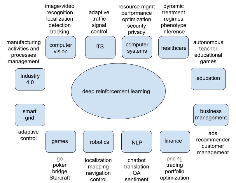
RL is usually for sequential decision making problems. However, some problems, seemingly non-sequential on surface, like machine translation and neural network architecture design, have been approached by RL. RL applications abound; and creativity would be the boundary.
Reinforcement learning is widely used in operations research (Powell, 2011), e.g., supply chain, inventory management, resource management, etc; we do not list it as an application area — it is implicitly a component in application areas like intelligent transportation system and Industry 4.0. We do not list smart city, an important application area of AI, as it includes several application areas here: healthcare, intelligent transportation system, smart grid, etc. We do not discuss some interesting applications, like music generation (Briot et al., 2017; Jaques et al., 2017), and retrosynthesis (Segler et al., 2017). See previous work on lists of RL applications at: http://bit.ly/2pDEs1Q, and http://bit.ly/2rjsmaz. We may only touch the surface of some application areas. It is desirable to do a deeper analysis of all application areas listed in the following, which we leave as a future work.
5.1 Games
Games provide excellent testbeds for RL/AI algorithms. We discuss Deep Q-Network (DQN) in Section 3.1.1 and its extensions, all of which experimented with Atari games. We discuss Mnih et al. (2016) in Section 3.2.1, Jaderberg et al. (2017) in Section 4.2, and Mirowski et al. (2017) in Section 5.2, and they used Labyrinth as the testbed. See Yannakakis and Togelius (2018) for a book on artificial intelligence and games. We discuss multi-agent RL in Section 4.4, which is at the intersection of game theory and RL/AI.
Backgammon and computer Go are perfect information board games. In Section 5.1.1, we discuss briefly Backgammon, and focus on computer Go, in particular, AlphaGo. Variants of card games, including majiang/mahjong, are imperfect information board games, which we discuss in Section 5.1.2, and focus on Texas Hold’em Poker. In video games, information may be perfect or imperfect, and game theory may be deployed or not. We discuss video games in Section 5.1.3. We will see more achievements in imperfect information games and video games, and their applications.
5.1.1 Perfect Information Board Games
Board games like Backgammon, Go, chess, checker and Othello, are classical testbeds for RL/AI algorithms. In such games, players reveal prefect information. Tesauro (1994) approached Backgammon by using neural networks to approximate value function learned with TD learning, and achieved human level performance. We focus on computer Go, in particular, AlphaGo (Silver et al., 2016a; 2017), for its significance.
Computer Go
The challenge of solving Computer Go comes from not only the gigantic search space of size , an astronomical number, but also the hardness of position evaluation (Müller, 2002), which was successfully used in solving many other games, like Backgammon and chess.
AlphaGo (Silver et al., 2016a), a computer Go program, won the human European Go champion, 5 games to 0, in October 2015, and became the first computer Go program to won a human professional Go player without handicaps on a full-sized 19 19 board. Soon after that in March 2016, AlphaGo defeated Lee Sedol, an 18-time world champion Go player, 4 games to 1, making headline news worldwide. This set a landmark in AI. AlphaGo defeated Ke Jie 3:0 in May 2017. AlphaGo Zero (Silver et al., 2017) further improved previous versions by learning a superhuman computer Go program without human knowledge.
AlphaGo: Training pipeline and MCTS
We discuss briefly how AlphaGo works based on Silver et al. (2016a) and Sutton and Barto (2018). See Sutton and Barto (2018) for a detailed and intuitive description of AlphaGo. See Deepmind’s description of AlphaGo at goo.gl/lZoQ1d.
AlphaGo was built with techniques of deep convolutional neural networks, supervised learning, reinforcement learning, and Monte Carlo tree search (MCTS) (Browne et al., 2012; Gelly and Silver, 2007; Gelly et al., 2012). AlphaGo is composed of two phases: neural network training pipeline and MCTS. The training pipeline phase includes training a supervised learning (SL) policy network from expert moves, a fast rollout policy, a RL policy network, and a RL value network.
The SL policy network has convolutional layers, ReLU nonlinearities, and an output softmax layer representing probability distribution over legal moves. The inputs to the CNN are 19 19 48 image stacks, where 19 is the dimension of a Go board and 48 is the number of features. State-action pairs are sampled from expert moves to train the network with stochastic gradient ascent to maximize the likelihood of the move selected in a given state. The fast rollout policy uses a linear softmax with small pattern features.
The RL policy network improves SL policy network, with the same network architecture, and the weights of SL policy network as initial weights, and policy gradient for training. The reward function is +1 for winning and -1 for losing in the terminal states, and 0 otherwise. Games are played between the current policy network and a random, previous iteration of the policy network, to stabilize the learning and to avoid overfitting. Weights are updated by stochastic gradient ascent to maximize the expected outcome.
The RL value network still has the same network architecture as SL policy network, except the output is a single scalar predicting the value of a position. The value network is learned in a Monte Carlo policy evaluation approach. To tackle the overfitting problem caused by strongly correlated successive positions in games, data are generated by self-play between the RL policy network and itself until game termination. The weights are trained by regression on state-outcome pairs, using stochastic gradient descent to minimize the mean squared error between the prediction and the corresponding outcome.
In MCTS phase, AlphaGo selects moves by lookahead search. It builds a partial game tree starting from the current state, in the following stages: 1) select a promising node to explore further, 2) expand a leaf node guided by the SL policy network and collected statistics, 3) evaluate a leaf node with a mixture of the RL value network and the rollout policy, 4) backup evaluations to update the action values. A move is then selected.
AlphaGo Zero
AlphaGo Zero can be understood as an approximation policy iteration, incorporating MCTS inside the training loop to perform both policy improvement and policy evaluation. MCTS may be regarded as a policy improvement operator. It outputs move probabilities stronger than raw probabilities of the neural network. Self-play with search may be regarded as a policy evaluation operator. It uses MCTS to select moves, and game winners as samples of value function. Then the policy iteration procedure updates the neural network’s weights to match the move probabilities and value more closely with the improved search probabilities and self-play winner, and conduct self-play with updated neural network weights in the next iteration to make the search stronger.
The features of AlphaGo Zero (Silver et al., 2017), comparing with AlphaGo (Silver et al., 2016a), are: 1) it learns from random play, with self-play reinforcement learning, without human data or supervision; 2) it uses black and white stones from the board as input, without any manual feature engineering; 3) it uses a single neural network to represent both policy and value, rather than separate policy network and value network; and 4) it utilizes the neural network for position evaluation and move sampling for MCTS, and it does not perform Monte Carlo rollouts. AlphaGo Zero deploys several recent achievements in neural networks: residual convolutional neural networks (ResNets), batch normalization, and rectifier nonlinearities.
AlphaGo Zero has three main components in its self-play training pipeline executed in parallel asynchronously: 1) optimize neural network weights from recent self-play data continually; 2) evaluate players continually; 3) use the strongest player to generate new self-play data.
When AlphaGo Zero playing a game against an opponent, MCTS searches from the current state, with the trained neural network weights, to generate move probabilities, and then selects a move.
We present a brief, conceptual pseudo code in Algorithm 9 for training in AlphaGo Zero, conducive for easier understanding. Refer to the original paper (Silver et al., 2017) for details.
Silver et al. (2017)
Discussions
AlphaGo Zero is a reinforcement learning algorithm. It is neither supervised learning nor unsupervised learning. The game score is a reward signal, not a supervision label. Optimizing the loss function is supervised learning. However, it performs policy evaluation and policy improvement, as one iteration in policy iteration.
AlphaGo Zero is not only a heuristic search algorithm. AlphaGo Zero is a policy iteration procedure, in which, heuristic search, in particular, MCTS, plays a critical role, but within the scheme of reinforcement learning policy iteration, as illustrated in the pseudo code in Algorithm 9. MCTS can be viewed as a policy improvement operator.
AlphaGo attains a superhuman level. It may confirm that professionals have developed effective strategies. However, it does not need to mimic professional plays. Thus it does not need to predict their moves correctly.
The inputs to AlphaGo Zero include the raw board representation of the position, its history, and the colour to play as 19 19 images; game rules; a game scoring function; invariance of game rules under rotation and reflection, and invariance to colour transposition except for komi. An additional and critical input is solid research and development experiences.
AlphaGo Zero utilized 64 GPU workers (each maybe with multiple GPUs) and 19 CPU parameter servers (each with multiple CPUs) for training, around 2000 TPUs for data generation, and 4 TPUs for game playing. The computation cost is too formidable for replicating AlphaGo Zero.
AlphaGo requires huge amount of data for training, so it is still a big data issue. However, the data can be generated by self play, with a perfect model or precise game rules.
Due to the perfect model or precise game rules for computer Go, AlphaGo algorithms have their limitations. For example, in healthcare, robotics and self driving problems, it is usually hard to collect a large amount of data, and it is hard or impossible to have a close enough or even perfect model. As such, it is nontrivial to directly apply AlphaGo algorithms to such applications.
On the other hand, AlphaGo algorithms, especially, the underlying techniques, namely, deep learning, reinforcement learning, and Monte Carlo tree search, have many applications. Silver et al. (2016a) and Silver et al. (2017) recommended the following applications: general game-playing (in particular, video games), classical planning, partially observed planning, scheduling, constraint satisfaction, robotics, industrial control, and online recommendation systems. AlphaGo Zero blog mentioned the following structured problems: protein folding, reducing energy consumption, and searching for revolutionary new materials.222Andrej Karpathy posted a blog titled ”AlphaGo, in context”, after AlphaGo defeated Ke Jie in May 2017. He characterized properties of Computer Go as: fully deterministic, fully observable, discrete action space, accessible perfect simulator, relatively short episode/game, clear and fast evaluation conducive for many trail-and-errors, and huge datasets of human play games, to illustrate the narrowness of AlphaGo. It is true that computer Go has limitations in the problem setting and thus potential applications, and is far from artificial general intelligence. However, we see the success of AlphaGo as the triumph of AI, in particular, AlphaGo’s underlying techniques, i.e., learning from demonstration (as supervised learning), deep learning, reinforcement learning, and Monte Carlo tree search; these techniques are present in many recent achievements in AI. As a whole technique, AlphaGo will probably shed lights on classical AI areas, like planning, scheduling, and constraint satisfaction (Silver et al., 2016a), and new areas for AI, like retrosynthesis (Segler et al., 2017). Reportedly, the success of AlphaGo’s conquering titanic search space inspired quantum physicists to solve the quantum many-body problem (Carleo and Troyer, 2017).
AlphaGo has made tremendous progress, and set a landmark in AI. However, we are still far away from attaining artificial general intelligence (AGI).
It is interesting to see how strong a raw deep neural network in AlphaGo can become, and how soon a very strong computer Go program would be available on a mobile phone.
5.1.2 Imperfect Information Board Games
Imperfect information games, or game theory in general, have many applications, e.g., security and medical decision support. It is interesting to see more progress of deep RL in such applications, and the full version of Texas Hold’em.
Heinrich and Silver (2016) proposed Neural Fictitious Self-Play (NFSP) to combine fictitious self-play with deep RL to learn approximate Nash equilibria for games of imperfect information in a scalable end-to-end approach without prior domain knowledge. NFSP was evaluated on two-player zero-sum games. In Leduc poker, NFSP approached a Nash equilibrium, while common RL methods diverged. In Limit Texas Hold’em, a real-world scale imperfect-information game, NFSP performed similarly to state-of-the-art, superhuman algorithms which are based on significant domain expertise.
Heads-up Limit Hold’em Poker was essentially solved (Bowling et al., 2015) with counterfactual regret minimization (CFR), which is an iterative method to approximate a Nash equilibrium of an extensive-form game with repeated self-play between two regret-minimizing algorithms.
DeepStack
Recently, significant progress has been made for Heads-up No-Limit Hold’em Poker (Moravčík et al., 2017), the DeepStack computer program defeated professional poker players for the first time. DeepStack utilized the recursive reasoning of CFR to handle information asymmetry, focusing computation on specific situations arising when making decisions and use of value functions trained automatically, with little domain knowledge or human expert games, without abstraction and offline computation of complete strategies as before.
5.1.3 Video Games
Video games would be great testbeds for artificial general intelligence.
Wu and Tian (2017) deployed A3C with CNN to train an agent in a partially observable 3D environment, Doom, from recent four raw frames and game variables, to predict next action and value function, following the curriculum learning (Bengio et al., 2009) approach of starting with simple tasks and gradually transition to harder ones. It is nontrivial to apply A3C to such 3D games directly, partly due to sparse and long term reward. The authors won the champion in Track 1 of ViZDoom Competition by a large margin, and plan the following future work: a map from an unknown environment, localization, a global plan to act, and visualization of the reasoning process.
Dosovitskiy and Koltun (2017) approached the problem of sensorimotor control in immersive environments with supervised learning, and won the Full Deathmatch track of the Visual Doom AI Competition. We list it here since it is usually a RL problem, yet it was solved with supervised learning. Lample and Chaplot (2017) also discussed how to tackle Doom.
Peng et al. (2017b) proposed a multiagent actor-critic framework, with a bidirectionally-coordinated network to form coordination among multiple agents in a team, deploying the concept of dynamic grouping and parameter sharing for better scalability. The authors used StarCraft as the testbed. Without human demonstration or labelled data as supervision, the proposed approach learned strategies for coordination similar to the level of experienced human players, like move without collision, hit and run, cover attack, and focus fire without overkill. Usunier et al. (2017); Justesen and Risi (2017) also studied StarCraft.
Oh et al. (2016) and Tessler et al. (2017) studied Minecraft, Chen and Yi (2017); Firoiu et al. (2017) studied Super Smash Bros, and Kansky et al. (2017) proposed Schema Networks and empirically studied variants of Breakout in Atari games.
See Justesen et al. (2017) for a survey about applying deep (reinforcement) learning to video games. See Ontañón et al. (2013) for a survey about Starcraft. Check AIIDE and CIG Starcraft AI Competitions, and its history at https://www.cs.mun.ca/~dchurchill/starcraftaicomp/history.shtml. See Lin et al. (2017) for StarCraft Dataset.
5.2 Robotics
Robotics is a classical area for reinforcement learning. See Kober et al. (2013) for a survey of RL in robotics, Deisenroth et al. (2013) for a survey on policy search for robotics, and Argall et al. (2009) for a survey of robot learning from demonstration. See the journal Science Robotics. It is interesting to note that from NIPS 2016 invited talk, Boston Dynamics robots did not use machine learning.
In the following, we discuss guided policy search (Levine et al., 2016a) and learn to navigate (Mirowski et al., 2017). See more recent robotics papers, e.g., Chebotar et al. (2016; 2017); Duan et al. (2017); Finn and Levine (2016); Gu et al. (2016a); Lee et al. (2017); Levine et al. (2016b); Mahler et al. (2017); Pérez-D’Arpino and Shah (2017); Popov et al. (2017); Yahya et al. (2016); Zhu et al. (2017b).
We recommend Pieter Abbeel’s NIPS 2017 Keynote Speech, Deep Learning for Robotics, slides at, https://www.dropbox.com/s/fdw7q8mx3x4wr0c/
5.2.1 Guided Policy Search
Levine et al. (2016a) proposed to train the perception and control systems jointly end-to-end, to map raw image observations directly to torques at the robot’s motors. The authors introduced guided policy search (GPS) to train policies represented as CNN, by transforming policy search into supervised learning to achieve data efficiency, with training data provided by a trajectory-centric RL method operating under unknown dynamics. GPS alternates between trajectory-centric RL and supervised learning, to obtain the training data coming from the policy’s own state distribution, to address the issue that supervised learning usually does not achieve good, long-horizon performance. GPS utilizes pre-training to reduce the amount of experience data to train visuomotor policies. Good performance was achieved on a range of real-world manipulation tasks requiring localization, visual tracking, and handling complex contact dynamics, and simulated comparisons with previous policy search methods. As the authors mentioned, ”this is the first method that can train deep visuomotor policies for complex, high-dimensional manipulation skills with direct torque control”.
5.2.2 Learn to Navigate
Mirowski et al. (2017) obtained the navigation ability by solving a RL problem maximizing cumulative reward and jointly considering un/self-supervised tasks to improve data efficiency and task performance. The authors addressed the sparse reward issues by augmenting the loss with two auxiliary tasks, 1) unsupervised reconstruction of a low-dimensional depth map for representation learning to aid obstacle avoidance and short-term trajectory planning; 2) self-supervised loop closure classification task within a local trajectory. The authors incorporated a stacked LSTM to use memory at different time scales for dynamic elements in the environments. The proposed agent learn to navigate in complex 3D mazes end-to-end from raw sensory input, and performed similarly to human level, even when start/goal locations change frequently.
In this approach, navigation is a by-product of the goal-directed RL optimization problem, in contrast to conventional approaches such as Simultaneous Localisation and Mapping (SLAM), where explicit position inference and mapping are used for navigation. This may have the chance to replace the popular SLAM, which usually requires manual processing.
5.3 Natural Language Processing
In the following we talk about natural language processing (NLP), dialogue systems in Section 5.3.1, machine translation in Section 5.3.2, and text generation in Section 5.3.3. There are many interesting issues in NLP, and we list some in the following.
Deep learning has been permeating into many subareas in NLP, and helping make significant progress. The above is a partial list. It appears that NLP is still a field, more about synergy than competition, for deep learning vs. non-deep learning algorithms, and for approaches based on no domain knowledge (end-to-end) vs linguistics knowledge. Some non-deep learning algorithms are effective and perform well, e.g., word2vec (Mikolov et al., 2013; 2017) and fastText (Joulin et al., 2017), and many works that study syntax and semantics of languages, see a recent example in semantic role labeling (He et al., 2017). Some deep learning approaches to NLP problems incorporate explicitly or implicitly linguistics knowledge, e.g., Socher et al. (2011; 2013); Yogatama et al. (2017). See an article by Christopher D. Manning, titled ”Last Words: Computational Linguistics and Deep Learning, A look at the importance of Natural Language Processing”, at http://mitp.nautil.us/article/170/last-words-computational-linguistics-and-deep-learning.
Melis et al. (2017)
5.3.1 Dialogue Systems
In dialogue systems, conversational agents, or chatbots, human and computer interacts with natural language. We intentionally remove ”spoken” before ”dialogue systems” to accommodate both spoken and written language user interface (UI). Jurafsky and Martin (2017) categorize dialogue systems as task-oriented dialog agents and chatbots; the former are set up to have short conversations to help complete particular tasks; the latter are set up to mimic human-human interactions with extended conversations, sometimes with entertainment value. As in Deng (2017), there are four categories: social chatbots, infobots (interactive question answering), task completion bots (task-oriented or goal-oriented) and personal assistant bots. We have seen generation one dialogue systems: symbolic rule/template based, and generation two: data driven with (shallow) learning. We are now experiencing generation three: data driven with deep learning, and reinforcement learning usually play an important role. A dialogue system usually include the following modules: (spoken) language understanding, dialogue manager (dialogue state tracker and dialogue policy learning), and a natural language generation (Young et al., 2013). In task-oriented systems, there is usually a knowledge base to query. A deep learning approach, as usual, attempts to make the learning of the system parameters end-to-end. See Deng (2017) for more details. See a survey paper on applying machine learning to speech recognition (Deng and Li, 2013).
Li et al. (2017b) presented an end-to-end task-completion neural dialogue system with parameters learned by supervised and reinforcement learning. The proposed framework includes a user simulator (Li et al., 2016d) and a neural dialogue system. The user simulator consists of user agenda modelling and natural language generation. The neural dialogue system is composed of language understanding and dialogue management (dialogue state tracking and policy learning). The authors deployed RL to train dialogue management end-to-end, representing the dialogue policy as a deep Q-network (Mnih et al., 2015), with the tricks of a target network and a customized experience replay, and using a rule-based agent to warm-start the system with supervised learning. The source code is available at http://github.com/MiuLab/TC-Bot.
Dhingra et al. (2017) proposed KB-InfoBot, a goal-oriented dialogue system for multi-turn information access. KB-InfoBot is trained end-to-end using RL from user feedback with differentiable operations, including those for accessing external knowledge database (KB). In previous work, e.g., Li et al. (2017b) and Wen et al. (2017), a dialogue system accesses real world knowledge from KB by symbolic, SQL-like operations, which is non-differentiable and disables the dialogue system from fully end-to-end trainable. KB-InfoBot achieved the differentiability by inducing a soft posterior distribution over the KB entries to indicate which ones the user is interested in. The authors designed a modified version of the episodic REINFORCE algorithm to explore and learn both the policy to select dialogue acts and the posterior over the KB entries for correct retrievals.The authors deployed imitation learning from rule-based belief trackers and policy to warm up the system.
Su et al. (2016b) proposed an on-line learning framework to train the dialogue policy jointly with the reward model via active learning with a Gaussian process model, to tackle the issue that it is unreliable and costly to use explicit user feedback as the reward signal. The authors showed empirically that the proposed framework reduced manual data annotations significantly and mitigated noisy user feedback in dialogue policy learning.
Li et al. (2016c) proposed to use deep RL to generate dialogues to model future reward for better informativity, coherence, and ease of answering, to attempt to address the issues in the sequence to sequence models based on Sutskever et al. (2014): the myopia and misalignment of maximizing the probability of generating a response given the previous dialogue turn, and the infinite loop of repetitive responses. The authors designed a reward function to reflect the above desirable properties, and deployed policy gradient to optimize the long term reward. It would be interesting to investigate the reward model with the approach in Su et al. (2016b) or with inverse RL and imitation learning as discussed in Section 3.3, although Su et al. (2016b) mentioned that such methods are costly, and humans may not act optimally.
Some recent papers follow: Asri et al. (2016), Bordes et al. (2017), Chen et al. (2016c), Eric and Manning (2017), Fatemi et al. (2016), Kandasamy et al. (2017), Lewis et al. (2017), Li et al. (2016a), Li et al. (2017a), Li et al. (2017b), Lipton et al. (2016), Mesnil et al. (2015), Mo et al. (2016), Peng et al. (2017a), Saon et al. (2016), Serban et al. (2017), Shah et al. (2016), She and Chai (2017), Su et al. (2016a), Weiss et al. (2017), Wen et al. (2015a), Wen et al. (2017), Williams and Zweig (2016), Williams et al. (2017), Xiong et al. (2017b), Xiong et al. (2017), Yang et al. (2016), Zhang et al. (2017a), Zhang et al. (2017c), Zhao and Eskenazi (2016), Zhou et al. (2017). See Serban et al. (2015) for a survey of corpora for building dialogue systems.
See NIPS 2016 Workshop on End-to-end Learning for Speech and Audio Processing, and NIPS 2015 Workshop on Machine Learning for Spoken Language Understanding and Interactions.
5.3.2 Machine Translation
Neural machine translation (Kalchbrenner and Blunsom, 2013; Cho et al., 2014; Sutskever et al., 2014; Bahdanau et al., 2015) utilizes end-to-end deep learning for machine translation, and becomes dominant, against the traditional statistical machine translation techniques. The neural machine translation approach usually first encodes a variable-length source sentence, and then decodes it to a variable-length target sentence. Cho et al. (2014) and Sutskever et al. (2014) used two RNNs to encode a sentence to a fix-length vector and then decode the vector into a target sentence. Bahdanau et al. (2015) introduced the soft-attention technique to learn to jointly align and translate.
He et al. (2016a) proposed dual learning mechanism to tackle the data hunger issue in machine translation, inspired by the observation that the information feedback between the primal, translation from language A to language B, and the dual, translation from B to A, can help improve both translation models, with a policy gradient method, using the language model likelihood as the reward signal. Experiments showed that, with only 10% bilingual data for warm start and monolingual data, the dual learning approach performed comparably with previous neural machine translation methods with full bilingual data in English to French tasks. The dual learning mechanism may have extensions to many tasks, if the task has a dual form, e.g., speech recognition and text to speech, image caption and image generation, question answering and question generation, search and keyword extraction, etc.
See Wu et al. (2016); Johnson et al. (2016) for Google’s Neural Machine Translation System; Gehring et al. (2017) for convolutional sequence to sequence learning for fast neural machine translation; Klein et al. (2017) for OpenNMT, an open source neural machine translation system; Cheng et al. (2016) for semi-supervised learning for neural machine translation, and Wu et al. (2017c) for adversarial neural machine translation. See Vaswani et al. (2017) for a new approach for translation that replaces CNN and RNN with attention and positional encoding. See Zhang et al. (2017b) for an open source toolkit for neural machine translation. See Monroe (2017) for a gentle introduction to translation.
Artetxe et al. (2017)
5.3.3 Text Generation
Text generation is the basis for many NLP problems, like conversational response generation, machine translation, abstractive summarization, etc.
Text generation models are usually based on -gram, feed-forward neural networks, or recurrent neural networks, trained to predict next word given the previous ground truth words as inputs; then in testing, the trained models are used to generate a sequence word by word, using the generated words as inputs. The errors will accumulate on the way, causing the exposure bias issue. Moreover, these models are trained with word level losses, e.g., cross entropy, to maximize the probability of next word; however, the models are evaluated on a different metrics like BLEU.
Ranzato et al. (2016) proposed Mixed Incremental Cross-Entropy Reinforce (MIXER) for sequence prediction, with incremental learning and a loss function combining both REINFORCE and cross-entropy. MIXER is a sequence level training algorithm, aligning training and testing objective, such as BLEU, rather than predicting the next word as in previous works.
Bahdanau et al. (2017) proposed an actor-critic algorithm for sequence prediction, attempting to further improve Ranzato et al. (2016). The authors utilized a critic network to predict the value of a token, i.e., the expected score following the sequence prediction policy, defined by an actor network, trained by the predicted value of tokens. Some techniques are deployed to improve performance: SARSA rather than Monter-Carlo method to lessen the variance in estimating value functions; target network for stability; sampling prediction from a delayed actor whose weights are updated more slowly than the actor to be trained, to avoid the feedback loop when actor and critic need to be trained based on the output of each other; reward shaping to avoid the issue of sparse training signal.
5.4 Computer Vision
Computer vision is about how computers gain understanding from digital images or videos. In the following, after presenting background in computer vision, we discuss recognition, motion analysis, scene understanding, integration with NLP, and visual control.
Reinforcement learning would be an important ingredient for interactive perception (Bohg et al., 2017), where perception and interaction with the environment would be helpful to each other, in tasks like object segmentation, articulation model estimation, object dynamics learning and haptic property estimation, object recognition or categorization, multimodal object model learning, object pose estimation, grasp planning, and manipulation skill learning.
More topics about applying deep RL to computer vision:
-
•
Liu et al. (2017) for semantic parsing of large-scale 3D point clouds;
-
•
Devrim Kaba et al. (2017) for view planning, which is a set cover problem;
-
•
Cao et al. (2017) for face hallucination, i.e., generating a high-resolution face image from a low-resolution input image;
-
•
Brunner et al. (2018) for learning to read maps;
-
•
Bhatti et al. (2016) for SLAM-augmented DQN.
5.4.1 Background
Todo: AlexNet (Krizhevsky et al., 2012), ResNets (He et al., 2016d) DenseNets (Huang et al., 2017), Fast R-CNN (Girshick, 2015), Faster R-CNN Ren et al. (2015), Mask R-CNN He et al. (2017), Shrivastava et al. (2017), VAEs (variational autoencoder) (Diederik P Kingma, 2014)
Todo: GANs (Goodfellow et al., 2014; Goodfellow, 2017); CycleGAN (Zhu et al., 2017a), DualGAN (Yi et al., 2017); See Arjovsky et al. (2017) for Wasserstein GAN (WGAN) as a stable GANs model. Gulrajani et al. (2017) proposed to improve stability of WGAN by penalizing the norm of the gradient of the discriminator with respect to its input, instead of clipping weights as in Arjovsky et al. (2017). Mao et al. (2016) proposed Least Squares GANs (LSGANs), another stable model.
Connection with RL: Finn et al. (2016a) established a connection between GANs, inverse RL, and energy-based models. Pfau and Vinyals (2016) established the connection between GANs and actor-critic algorithms. Ho and Ermon (2016) and Li et al. (2017) studied the connection between GANs and imitation learning.
autoencoder (Hinton and Salakhutdinov, 2006)
For disentangled factor learning, Kulkarni et al. (2015) proposed DC-IGN, the Deep Convolution Inverse Graphics Network, which follows a semi-supervised way; and Chen et al. (2016a) proposed InfoGAN, an information-theoretic extension to the Generative Adversarial Network, which follows an unsupervised way. Zhou et al. (2015) showed that object detectors emerge from learning to recognize scenes, without supervised labels for objects.
Higgins et al. (2017) proposed -VAE to automatically discover interpretable, disentangled, factorised, latent representations from raw images in an unsupervised way. The hyperparameter balances latent channel capacity and independence constraints with reconstruction accuracy. When , -VAE is the same as the original VAEs.
Eslami et al. (2016) proposed the framework of Attend-Infer-Repeat for efficient inference in structured image models to reason about objects explicitly. The authors deployed a recurrent neural network to design an iterative process for inference, by attending to one object at a time, and for each image, learning an appropriate number of inference steps. The authors showed that, in an unsupervised way, the proposed approach can learn generative models to identify multiple objects for both 2D and 3D problems.
Zhang and Zhu (2018) surveyed visual interpretability for deep learning.
5.4.2 Recognition
RL can improve efficiency for image classification by focusing only on salient parts. For visual object localization and detection, RL can improve efficiency over approaches with exhaustive spatial hypothesis search and sliding windows, and strikes a balance between sampling more regions for better accuracy and stopping the search when sufficient confidence is obtained about the target’s location.
Mnih et al. (2014) introduced the recurrent attention model (RAM) to focus on selected sequence of regions or locations from an image or video for image classification and object detection. The authors used REINFORCE to train the model, to overcome the issue that the model is non-differentiable, and experimented on an image classification task and a dynamic visual control problem.
Caicedo and Lazebnik (2015) proposed an active detection model for object localization with DQN, by deforming a bounding box with transformation actions to determine the most specific location for target objects. Jie et al. (2016) proposed a tree-structure RL approach to search for objects sequentially, considering both the current observation and previous search paths, by maximizing the long-term reward associated with localization accuracy over all objects with DQN. Mathe et al. (2016) proposed to use policy search for visual object detection. Kong et al. (2017) deployed collaborative multi-agent RL with inter-agent communication for joint object search. Welleck et al. (2017) proposed a hierarchical visual architecture with an attention mechanism for multi-label image classification. Rao et al. (2017) proposed an attention-aware deep RL method for video face recognition.
Krull et al. (2017) for 6D object pose estimation
5.4.3 Motion Analysis
In tracking, an agent needs to follow a moving object. Supančič and Ramanan (2017) proposed online decision-making process for tracking, formulated it as a partially observable decision-making process (POMDP), and learned policies with deep RL algorithms, to decide where to look for the object, when to reinitialize, and when to update the appearance model for the object, where image frames may be ambiguous and computational budget may be constrained. Yun et al. (2017) also studied visual tracking with deep RL.
Rhinehart and Kitani (2017) proposed Discovering Agent Rewards for K-futures Online (DARKO) to model and forecast first-person camera wearer’s long-term goals, together with states, transitions, and rewards from streaming data, with online inverse reinforcement learning.
5.4.4 Scene Understanding
Wu et al. (2017b) studied the problem of scene understanding, and attempted to obtain a compact, expressive, and interpretable representation to encode scene information like objects, their categories, poses, positions, etc, in a semi-supervised way. In contrast to encoder-decoder based neural architectures as in previous works, Wu et al. (2017b) proposed to replace the decoder with a deterministic rendering function, to map a structured and disentangled scene description, scene XML, to an image; consequently, the encoder transforms an image to the scene XML by inverting the rendering operation, a.k.a., de-rendering. The authors deployed a variant of REINFORCE algorithm to overcome the non-differentiability issue of graphics rendering engines.
Wu et al. (2017a) proposed a paradigm with three major components, a convolutional perception module, a physics engine, and a graphics engine, to understand physical scenes without human annotations. The perception module recovers a physical world representation by inverting the graphics engine, inferring the physical object state for each segment proposal in input and combining them. The generative physics and graphics engines then run forward with the world representation to reconstruct the visual data. The authors showed results on both neural, differentiable and more mature but non-differentiable physics engines.
5.4.5 Integration with NLP
Some are integrating computer vision with natural language processing. Xu et al. (2015) integrated attention to image captioning, trained the hard version attention with REINFORCE, and showed the effectiveness of attention on Flickr8k, Flickr30k, and MS COCO datasets. Rennie et al. (2017) introduced self-critical sequence training, using the output of test-time inference algorithm as the baseline in REINFORCE to normalize the rewards it experiences, for image captioning. See also Liu et al. (2016), Lu et al. (2016), and Ren et al. (2017) for image captioning. Strub et al. (2017) proposed end-to-end optimization with deep RL for goal-driven and visually grounded dialogue systems for GuessWhat?! game. Das et al. (2017) proposed to learn cooperative Visual Dialog agents with deep RL. See also Kottur et al. (2017). See Pasunuru and Bansal (2017) for video captioning. See Liang et al. (2017d) for visual relationship and attribute detection.
5.4.6 Visual Control
Visual control is about deriving a policy from visual inputs, e.g., in games (Mnih et al., 2015; Silver et al., 2016a; 2017; Oh et al., 2015; Wu and Tian, 2017; Dosovitskiy and Koltun, 2017; Lample and Chaplot, 2017; Jaderberg et al., 2017), robotics (Finn and Levine, 2016; Gupta et al., 2017b; Lee et al., 2017; Levine et al., 2016a; Mirowski et al., 2017; Zhu et al., 2017b), and self-driving vehicles (Bojarski et al., 2016; 2017; Zhou and Tuzel, 2017). 333Although we include visual control here, it is not very clear if we should categorize the following type of problems, e.g., DQN (Mnih et al., 2015) and AlphaGo (Silver et al., 2016a; 2017), into computer vision: pixels (DQN) or problem setting (Go board status) as the input, some deep neural networks as the architecture, and an end-to-end gradient descent/ascent algorithm as the optimization method to find a policy, without any further knowledge of computer vision. Or we may see this as part of the synergy of computer vision and reinforcement learning.
5.5 Business Management
Reinforcement learning has many applications in business management, like ads, recommendation, customer management, and marketing.
Li et al. (2010) formulated personalized news articles recommendation as a contextual bandit problem, to learn an algorithm to select articles sequentially for users based on contextual information of the user and articles, such as historical activities of the user and descriptive information and categories of content, and to take user-click feedback to adapt article selection policy to maximize total user clicks in the long run.
Theocharous et al. (2015) formulated a personalized ads recommendation systems as a RL problem to maximize life-time value (LTV) with theoretical guarantees. This is in contrast to a myopic solution with supervised learning or contextual bandit formulation, usually with the performance metric of click through rate (CTR). As the models are hard to learn, the authors deployed a model-free approach to compute a lower-bound on the expected return of a policy to address the off-policy evaluation problem, i.e., how to evaluate a RL policy without deployment.
Li et al. (2015) also attempted to maximize lifetime value of customers. Silver et al. (2013) proposed concurrent reinforcement learning for the customer interaction problem. See Sutton and Barto (2018) for a detailed and intuitive description of some topics discussed here under the section title of Personalized Web Services.
5.6 Finance
RL is a natural solution to some finance and economics problems (Hull, 2014; Luenberger, 1997), like option pricing (Longstaff and Schwartz, 2001; Tsitsiklis and Van Roy, 2001; Li et al., 2009), and multi-period portfolio optimization (Brandt et al., 2005; Neuneier, 1997), where value function based RL methods were used. Moody and Saffell (2001) proposed to utilize policy search to learn to trade; Deng et al. (2016) extended it with deep neural networks. Deep (reinforcement) learning would provide better solutions in some issues in risk management (Hull, 2014; Yu et al., 2009). The market efficiency hypothesis is fundamental in finance. However, there are well-known behavioral biases in human decision-making under uncertainty, in particular, prospect theory (Prashanth et al., 2016). A reconciliation is the adaptive markets hypothesis (Lo, 2004), which may be approached by reinforcement learning.
It is nontrivial for finance and economics academia to accept blackbox methods like neural networks; Heaton et al. (2016) may be regarded as an exception. However, there is a lecture in AFA 2017 annual meeting: Machine Learning and Prediction in Economics and Finance. We may also be aware that financial firms would probably hold state-of-the-art research/application results.
5.7 Healthcare
There are many opportunities and challenges in healthcare for machine learning (Miotto et al., 2017; Saria, 2014). Personalized medicine is getting popular in healthcare. It systematically optimizes the patient’s health care, in particular, for chronic conditions and cancers using individual patient information, potentially from electronic health/medical record (EHR/EMR). Dynamic treatment regimes (DTRs) or adaptive treatment strategies are sequential decision making problems. Some issues in DTRs are not in standard RL. Shortreed et al. (2011) tackled the missing data problem, and designed methods to quantify the evidence of the learned optimal policy. Goldberg and Kosorok (2012) proposed methods for censored data (patients may drop out during the trial) and flexible number of stages. See Chakraborty and Murphy (2014) for a recent survey, and Kosorok and Moodie (2015) for an edited book about recent progress in DTRs. Currently Q-learning is the RL method in DTRs. Ling et al. (2017) applied deep RL to the problem of inferring patient phenotypes.
Some recent workshops at the intersection of machine learning and healthcare are: NIPS 2016 Workshop on Machine Learning for Health (http://www.nipsml4hc.ws) and NIPS 2015 Workshop on Machine Learning in Healthcare (https://sites.google.com/site/nipsmlhc15/). See ICML 2017 Tutorial on Deep Learning for Health Care Applications: Challenges and Solutions (https://sites.google.com/view/icml2017-deep-health-tutorial/home).
5.8 Education
Mandel et al. (2014)
Liu et al. (2014)
5.9 Industry 4.0
The ear of Industry 4.0 is approaching, e.g., see O’Donovan et al. (2015), and Preuveneers and Ilie-Zudor (2017). Reinforcement learning in particular, artificial intelligence in general, will be critical enabling techniques for many aspects of Industry 4.0, e.g., predictive maintenance, real-time diagnostics, and management of manufacturing activities and processes. Robots will prevail in Industry 4.0, and we discuss robotics in Section 5.2.
Liu and Tomizuka (2016; 2017) studied how to make robots and people to collaborate to achieve both flexibility and productivity in production lines. See a blog titled Towards Intelligent Industrial Co-robots, at http://bair.berkeley.edu/blog/2017/12/12/corobots/
Hein et al. (2017) designed a benchmark for the RL community to attempt to bridge the gap between academic research and real industrial problems. Its open source based on OpenAI Gym is available at https://github.com/siemens/industrialbenchmark.
Surana et al. (2016) proposed to apply guided policy search (Levine et al., 2016a) as discussed in Section 5.2.1 to optimize trajectory policy of cold spray nozzle dynamics, to handle complex trajectories traversing by robotic agents. The authors generated cold spray surface simulation profiles to train the model.
5.10 Smart Grid
A smart grid is a power grid utilizing modern information technologies to create an intelligent electricity delivery network for electricity generation, transmission, distribution, consumption, and control (Fang et al., 2012). An important aspect is adaptive control (Anderson et al., 2011). Glavic et al. (2017) reviewed application of RL for electric power system decision and control. Here we briefly discuss demand response (Wen et al., 2015b; Ruelens et al., 2016).
Demand response systems motivate users to dynamically adapt electrical demands in response to changes in grid signals, like electricity price, temperature, and weather, etc. With suitable electricity prices, load of peak consumption may be rescheduled/lessened, to improve efficiency, reduce costs, and reduce risks. Wen et al. (2015b) proposed to design a fully automated energy management system with model-free reinforcement learning, so that it doesn’t need to specify a disutility function to model users’ dissatisfaction with job rescheduling. The authors decomposed the RL formulation over devices, so that the computational complexity grows linearly with the number of devices, and conducted simulations using Q-learning. Ruelens et al. (2016) tackled the demand response problem with batch RL. Wen et al. (2015b) took the exogenous prices as states, and Ruelens et al. (2016) utilized the average as feature extractor to construct states.
5.11 Intelligent Transportation Systems
Intelligent transportation systems (Bazzan and Klügl, 2014) apply advanced information technologies for tackling issues in transport networks, like congestion, safety, efficiency, etc., to make transport networks, vehicles and users smart.
An important issue in intelligent transportation systems is adaptive traffic signal control. El-Tantawy et al. (2013) proposed to model the adaptive traffic signal control problem as a multiple player stochastic game, and solve it with the approach of multi-agent RL (Shoham et al., 2007; Busoniu et al., 2008). Multi-agent RL integrates single agent RL with game theory, facing challenges of stability, nonstationarity, and curse of dimensionality. El-Tantawy et al. (2013) approached the issue of coordination by considering agents at neighbouring intersections. The authors validated their proposed approach with simulations, and real traffic data from the City of Toronto. El-Tantawy et al. (2013) didn’t explore function approximation. See also van der Pol and Oliehoek (2017) for a recent work, and Mannion et al. (2016) for an experimental review, about applying RL to adaptive traffic signal control.
Self-driving vehicle is also a topic of intelligent transportation systems. See Bojarski et al. (2016), Bojarski et al. (2017), Zhou and Tuzel (2017).
See NIPS 2017, 2016 Workshop on Machine Learning for Intelligent Transportation Systems. Check for a special issue of IEEE Transactions on Neural Networks and Learning Systems on Deep Reinforcement Learning and Adaptive Dynamic Programming, tentative publication date December 2017.
5.12 Computer Systems
Computer systems are indispensable in our daily life and work, e.g., mobile phones, computers, and cloud computing. Control and optimization problems abound in computer systems, e,g., Mestres et al. (2016) proposed knowledge-defined networks, Gavrilovska et al. (2013) reviewed learning and reasoning techniques in cognitive radio networks, and Haykin (2005) discussed issues in cognitive radio, like channel state prediction and resource allocation. We also note that Internet of Things (IoT)(Xu et al., 2014) and wireless sensor networks (Alsheikh et al., 2014) play an important role in Industry 4.0 as discussed in Section 5.9, in Smart Grid as discussed in Section 5.10, and in Intelligent Transportation Systems as discussed in Section 5.11.
5.12.1 Resource Allocation
Mao et al. (2016) studied resource management in systems and networking with deep RL. The authors proposed to tackle multi-resource cluster scheduling with policy gradient, in an online manner with dynamic job arrivals, optimizing various objectives like average job slowdown or completion time. The authors validated their proposed approach with simulation.
Liu et al. (2017) proposed a hierarchical framework to tackle resource allocation and power management in cloud computing with deep RL. The authors decomposed the problem as a global tier for virtual machines resource allocation and a local tier for servers power management. The authors validated their proposed approach with actual Google cluster traces. Such hierarchical framework/decomposition approach was to reduce state/action space, and to enable distributed operation of power management.
Google deployed machine learning for data centre power management, reducing energy consumption by 40%, https://deepmind.com/blog/deepmind-ai-reduces-google-data-centre-cooling-bill-40/. Optimizing memory control is discussed in Sutton and Barto (2018).
5.12.2 Performance Optimization
Mirhoseini et al. (2017) proposed to optimize device placement for Tensorflow computational graphs with RL. The authors deployed a seuqence-to-sequence model to predict how to place subsets of operations in a Tensorflow graph on available devices, using the execution time of the predicted placement as reward signal for REINFORCE algorithm. The proposed method found placements of Tensorflow operations on devices for Inception-V3, recurrent neural language model and neural machine translation, yielding shorter execution time than those placements designed by human experts. Computation burden is one concern for a RL approach to search directly in the solution space of a combinatorial problem. We discuss combinatorial optimization in Section LABEL:combinatorial.
5.12.3 Security & Privacy
adversarial attacks, e.g., Huang et al. (2017),
http://rll.berkeley.edu/adversarial/
Papernot et al. (2016)
Abadi et al. (2016)
Balle et al. (2016)
Delle Fave et al. (2014)
Carlini and Wagner (2017b)
defenders Ian J. Goodfellow (2015); Carlini and Wagner (2017a); Madry et al. (2017); Tramèr et al. (2017)
Anderson et al. (2017) https://github.com/endgameinc/gym-malware
Evtimov et al. (2017) See a blog titled Physical Adversarial Examples Against Deep Neural Networks at http://bair.berkeley.edu/blog/2017/12/30/yolo-attack/, which contains a brief survey of attack and defence algorithms. Check ACM Conference on Computer and Communications Security (CCS 2016) tutorial on Adversarial Data Mining: Big Data Meets Cyber Security, https://www.sigsac.org/ccs/CCS2016/tutorials/index.html
6 More Topics
We list more interesting and/or important topics we have not discussed in this overview as below, hoping it would provide pointers for those who may be interested in studying them further. Some topics/papers may not contain RL yet. However, we believe these are interesting and/or important directions for RL in the sense of either theory or application. It would be definitely more desirable if we could finish reviewing these, however, we leave it as future work.
- •
-
•
interpretability, e.g., Al-Shedivat et al. (2017b); Doshi-Velez and Kim (2017); Harrison et al. (2017); Lei et al. (2016); Lipton (2016); Miller (2017); Ribeiro et al. (2016); Huk Park et al. (2016)
-
–
NIPS 2017 Interpretable Machine Learning Symposium
-
–
ICML 2017 Tutorial on Interpretable Machine Learning
-
–
NIPS 2016 Workshop on Interpretable ML for Complex Systems
-
–
ICML Workshop on Human Interpretability in Machine Learning 2017, 2016
-
–
-
•
usable machine learning, Bailis et al. (2017)
-
Cloud AutoML: Making AI accessible to every business,
https://www.blog.google/topics/google-cloud/cloud-automl-making-ai-accessible-every-business/ -
•
expressivity, Raghu et al. (2016)
-
•
testing, Pei et al. (2017)
- •
-
•
deep learning compression
- •
- •
- •
-
•
professor forcing, Lamb et al. (2016)
- •
- •
- •
-
•
safe RL, e.g., Berkenkamp et al. (2017)
-
•
agent modelling, e.g., Albrechta and Stone (2018)
- •
-
•
neural episodic control, Pritzel et al. (2017)
- •
- •
-
•
pathNet, Fernando et al. (2017)
- •
-
•
capsules, Sabour et al. (2017)
- •
-
•
deep probabilistic programming, Tran et al. (2017)
-
•
active learning, e.g., Fang et al. (2017)
-
•
deep learning games, Schuurmans and Zinkevich (2016)
- •
- •
- •
-
•
education, e.g.,
-
•
music generation, e.g., Jaques et al. (2017)
-
•
retrosynthesis, e.g., Segler et al. (2017)
-
•
quantum RL, e.g., Crawford et al. (2016)
-
–
NIPS 2015 Workshop on Quantum Machine Learning
-
–
7 Resources
We list a collection of deep RL resources including books, surveys, reports, online courses, tutorials, conferences, journals and workshops, blogs, testbed, and open source algorithm implementations. This by no means is complete.
It is essential to have a good understanding of reinforcement learning, before having a good understanding of deep reinforcement learning. We recommend to start with the textbook by Sutton and Barto (Sutton and Barto, 2018), the RL courses by Rich Sutton and by David Silver as the first two items in the Courses subsection below.
In the current information/social media age, we are overwhelmed by information, e.g., from Twitter, arXiv, Google+, etc. The skill to efficiently select the best information becomes essential. The Wild Week in AI (http://www.wildml.com) is an excellent series of weekly summary blogs. In an ear of AI, we expect to see an AI agent to do such tasks like intelligently searching and summarizing relevant news, blogs, research papers, etc.
7.1 Books
7.2 More Books
- •
-
•
an operations research oriented RL book (Powell, 2011)
-
•
an edited RL book (Wiering and van Otterlo, 2012)
-
•
Markov decision processes (Puterman, 2005)
- •
-
•
artificial intelligence (Russell and Norvig, 2009)
- •
-
•
semi-supervised learning (Zhu and Goldberg, 2009)
-
•
game theory (Leyton-Brown and Shoham, 2008)
7.3 Surveys and Reports
7.4 Courses
-
•
Richard Sutton, Reinforcement Learning, 2016, slides, assignments, reading materials, etc.
http://www.incompleteideas.net/sutton/609%20dropbox/ -
•
David Silver, Reinforcement Learning, 2015, slides (goo.gl/UqaxlO), video-lectures (goo.gl/7BVRkT)
-
•
Sergey Levine, John Schulman and Chelsea Finn, CS 294: Deep Reinforcement Learning, Spring 2017, http://rll.berkeley.edu/deeprlcourse/
-
•
Katerina Fragkiadaki, Ruslan Satakhutdinov, Deep Reinforcement Learning and Control, Spring 2017, https://katefvision.github.io
-
•
Emma Brunskill, CS234: Reinforcement Learning, http://web.stanford.edu/class/cs234/
-
•
Charles Isbell, Michael Littman and Pushkar Kolhe, Udacity: Machine Learning: Reinforcement Learning, goo.gl/eyvLfg
-
•
David Donoho, Hatef Monajemi, and Vardan Papyan, Theories of Deep Learning (Stanford STATS 385), https://stats385.github.io
-
•
Nando de Freitas, Deep Learning Lectures, https://www.youtube.com/user/ProfNandoDF
-
•
Fei-Fei Li, Andrej Karpathy and Justin Johnson, CS231n: Convolutional Neural Networks for Visual Recognition, http://cs231n.stanford.edu
-
•
Richard Socher, CS224d: Deep Learning for Natural Language Processing,
http://cs224d.stanford.edu -
•
Brendan Shillingford, Yannis Assael, Chris Dyer, Oxford Deep NLP 2017 course,
https://github.com/oxford-cs-deepnlp-2017 -
•
Pieter Abbeel, Advanced Robotics, Fall 2015, https://people.eecs.berkeley.edu/ pabbeel/cs287-fa15/
-
•
Emo Todorov, Intelligent control through learning and optimization,
http://homes.cs.washington.edu/ todorov/courses/amath579/index.html -
•
Abdeslam Boularias, Robot Learning Seminar, http://www.abdeslam.net/robotlearningseminar
-
•
MIT 6.S094: Deep Learning for Self-Driving Cars, http://selfdrivingcars.mit.edu
-
•
Jeremy Howard, Practical Deep Learning For Coders, http://course.fast.ai
-
•
Andrew Ng, Deep Learning Specialization
https://www.coursera.org/specializations/deep-learning
7.5 Tutorials
-
•
Rich Sutton, Introduction to Reinforcement Learning with Function Approximation, https://www.microsoft.com/en-us/research/video/tutorial-introduction-to-reinforcement-learning-with-function-approximation/
-
•
Deep Reinforcement Learning
-
–
David Silver, ICML 2016
-
–
David Silver, 2nd Multidisciplinary Conference on Reinforcement Learning and Decision Making (RLDM), Edmonton, Alberta, Canada, 2015;
http://videolectures.net/rldm2015_silver_reinforcement_learning/ -
–
John Schulman, Deep Learning School, 2016
-
–
Pieter Abbeel, Deep Learning Summer School, 2016;
http://videolectures.net/deeplearning2016_abbeel_deep_reinforcement/ -
–
Pieter Abbeel and John Schulman, Deep Reinforcement Learning Through Policy Optimization, NIPS 2016
-
–
Sergey Levine and Chelsea Finn, Deep Reinforcement Learning, Decision Making, and Control, ICML 2017
-
–
-
•
John Schulman, The Nuts and Bolts of Deep Reinforcement Learning Research, Deep Reinforcement Learning Workshop, NIPS 2016
-
•
Joelle Pineau, Introduction to Reinforcement Learning, Deep Learning Summer School, 2016; http://videolectures.net/deeplearning2016_pineau_reinforcement_learning/
-
•
Andrew Ng, Nuts and Bolts of Building Applications using Deep Learning, NIPS 2016
-
•
Deep Learning Summer School, 2016, 2015
-
•
Deep Learning and Reinforcement Learning Summer Schools, 2017
-
•
Simons Institute Interactive Learning Workshop, 2017
-
•
Simons Institute Representation Learning Workshop, 2017
-
•
Simons Institute Computational Challenges in Machine Learning Workshop, 2017
7.6 Conferences, Journals and Workshops
-
•
NIPS: Neural Information Processing Systems
-
•
ICML: International Conference on Machine Learning
-
•
ICLR: International Conference on Learning Representation
-
•
RLDM: Multidisciplinary Conference on Reinforcement Learning and Decision Making
-
•
EWRL: European Workshop on Reinforcement Learning
-
•
AAAI, IJCAI, ACL, EMNLP, SIGDIAL, ICRA, IROS, KDD, SIGIR, CVPR, etc.
-
•
Nature Machine Intelligence, Science Robotics, JMLR, MLJ, AIJ, JAIR, PAMI, etc
-
•
Nature May 2015, Science July 2015, survey papers on machine learning/AI
-
•
Science, July 7, 2017 issue, The Cyberscientist, a special issue about AI
-
•
Deep Reinforcement Learning Workshop, NIPS 2016, 2015; IJCAI 2016
-
•
Deep Learning Workshop, ICML 2016
-
•
http://distill.pub
7.7 Blogs
-
•
Deepmind Blog, https://deepmind.com/blog/
-
-
-
•
Google Research Blog, https://research.googleblog.com, goo.gl/ok88b7
-
The Google Brain Team — Looking Back on 2017, goo.gl/1G7jnb, goo.gl/uCWDLr
-
The Google Brain Team — Looking Back on 2016,
-
•
Berkeley AI Research Blog, http://bair.berkeley.edu/blog/
-
•
OpenAI Blog, https://blog.openai.com
-
•
Marc Bellemare, Classic and modern reinforcement learning,
http://www.marcgbellemare.info/blog/ -
•
Denny Britz, The Wild Week in AI, a weekly AI & deep learning newsletter, www.wildml.com, esp. goo.gl/MyrwDC
-
•
Andrej Karpathy, karpathy.github.io, esp. goo.gl/1hkKrb
-
•
Junling Hu, Reinforcement learning explained - learning to act based on long-term payoffs
https://www.oreilly.com/ideas/reinforcement-learning-explained -
•
Li Deng, How deep reinforcement learning can help chatbots
https://venturebeat.com/2016/08/01/how-deep-reinforcement-learning-can-help-chatbots/ -
•
Reinforcement Learning, https://www.technologyreview.com/s/603501/10-breakthrough-technologies-2017-reinforcement-learning/
-
•
Deep Learning, https://www.technologyreview.com/s/513696/deep-learning/
7.8 Testbeds
- •
-
•
Ray RLlib: A Composable and Scalable Reinforcement Learning Library (Liang et al., 2017c), http://ray.readthedocs.io/en/latest/rllib.html
-
•
OpenAI Gym (https://gym.openai.com) is a toolkit for the development of RL algorithms, consisting of environments, e.g., Atari games and simulated robots, and a site for the comparison and reproduction of results.
-
•
OpenAI Universe (https://universe.openai.com) is used to turn any program into a Gym environment. Universe has already integrated many environments, including Atari games, flash games, browser tasks like Mini World of Bits and real-world browser tasks. Recently, GTA V was added to Universe for self-driving vehicle simulation.
-
•
DeepMind Control Suite, Tassa et al. (2018)
-
•
DeepMind released a first-person 3D game platform DeepMind Lab (Beattie et al., 2016). Deepmind and Blizzard will collaborate to release the Starcraft II AI research environment (goo.gl/Ptiwfg).
-
•
Psychlab: A Psychology Laboratory for Deep Reinforcement Learning Agents (Leibo et al., 2018)
-
•
FAIR TorchCraft (Synnaeve et al., 2016) is a library for Real-Time Strategy (RTS) games such as StarCraft: Brood War.
-
•
Deepmind PySC2 - StarCraft II Learning Environment, https://github.com/deepmind/pysc2
-
•
David Churchill, CommandCenter: StarCraft 2 AI Bot,
https://github.com/davechurchill/commandcenter -
•
ParlAI is a framework for dialogue research, implemented in Python, open-sourced by Facebook. https://github.com/facebookresearch/ParlAI
-
•
ELF, an extensive, lightweight and flexible platform for RL research (Tian et al., 2017)
-
•
Project Malmo (https://github.com/Microsoft/malmo), from Microsoft, is an AI research and experimentation platform built on top of Minecraft.
-
•
Twitter open-sourced torch-twrl, a framework for RL development.
-
•
ViZDoom is a Doom-based AI research platform for visual RL (Kempka et al., 2016).
-
•
Baidu Apollo Project, self-driving open-source, http://apollo.auto
-
•
TORCS is a car racing simulator (Bernhard Wymann et al., 2014).
-
•
MuJoCo, Multi-Joint dynamics with Contact, is a physics engine, http://www.mujoco.org.
-
•
Nogueira and Cho (2016) presented WebNav Challenge for Wikipedia links navigation.
-
•
RLGlue (Tanner and White, 2009) is a language-independent software for RL experiments. It may need extensions to accommodate progress in deep learning.
-
•
RLPy (Geramifard et al., 2015) is a value-function-based reinforcement learning framework for education and research.
7.9 Algorithm Implementations
We collect implementations of algorithms, either classical ones as in a textbook like Sutton and Barto (2018) or in recent papers.
-
•
Shangtong Zhang, Python code to accompany Sutton & Barto’s RL book and David Silver’s RL course, https://github.com/ShangtongZhang/reinforcement-learning-an-introduction
-
•
Learning Reinforcement Learning (with Code, Exercises and Solutions),
http://www.wildml.com/2016/10/learning-reinforcement-learning/ -
•
OpenAI Baselines: high-quality implementations of reinforcement learning algorithms, https://github.com/openai/baselines
-
•
TensorFlow implementation of Deep Reinforcement Learning papers,
https://github.com/carpedm20/deep-rl-tensorflow -
•
Deep reinforcement learning for Keras, https://github.com/matthiasplappert/keras-rl
-
•
Code Implementations for NIPS 2016 papers, http://bit.ly/2hSaOyx
-
•
Benchmark results of various policy optimization algorithms (Duan et al., 2016),
https://github.com/rllab/rllab - •
-
•
DQN (Mnih et al., 2015), https://sites.google.com/a/deepmind.com/dqn/
-
•
Tensorflow implementation of DQN (Mnih et al., 2015),
https://github.com/devsisters/DQN-tensorflow -
•
Deep Q Learning with Keras and Gym, https://keon.io/deep-q-learning/
-
•
Deep Exploration via Bootstrapped DQN (Osband et al., 2016), a Torch implementation, https://github.com/iassael/torch-bootstrapped-dqn
-
•
DarkForest, the Facebook Go engine (Github), https://github.com/facebookresearch/darkforestGo
-
•
Using Keras and Deep Q-Network to Play FlappyBird,
https://yanpanlau.github.io/2016/07/10/FlappyBird-Keras.html -
•
Deep Deterministic Policy Gradients (Lillicrap et al., 2016) in TensorFlow,
http://pemami4911.github.io/blog/2016/08/21/ddpg-rl.html -
•
Deep Deterministic Policy Gradient (Lillicrap et al., 2016) to play TORCS,
https://yanpanlau.github.io/2016/10/11/Torcs-Keras.html -
•
Reinforcement learning with unsupervised auxiliary tasks (Jaderberg et al., 2017),
https://github.com/miyosuda/unreal -
•
Learning to communicate with deep multi-agent reinforcement learning,
https://github.com/iassael/learning-to-communicate -
•
Deep Reinforcement Learning: Playing a Racing Game - Byte Tank, http://bit.ly/2pVIP4i
-
•
Differentiable Neural Computer (DNC) (Graves et al., 2016),
https://github.com/deepmind/dnc -
•
Playing FPS Games with Deep Reinforcement Learning (Lample and Chaplot, 2017),
https://github.com/glample/Arnold -
•
Learning to Learn (Reed and de Freitas, 2016) in TensorFlow,
https://github.com/deepmind/learning-to-learn -
•
Value Iteration Networks (Tamar et al., 2016) in Tensorflow,
https://github.com/TheAbhiKumar/tensorflow-value-iteration-networks -
•
Tensorflow implementation of the Predictron (Silver et al., 2016b),
https://github.com/zhongwen/predictron -
•
Meta Reinforcement Learning (Wang et al., 2016) in Tensorflow,
https://github.com/awjuliani/Meta-RL - •
-
•
Starter code for evolution strategies (Salimans et al., 2017),
https://github.com/openai/evolution-strategies-starter - •
-
•
DeepForest (Zhou and Feng, 2017), http://lamda.nju.edu.cn/files/gcforest.zip
8 Brief Summary
We list some RL issues and corresponding proposed approaches covered in this overview, as well as some classical work. One direction of future work is to further refine this section, especially for issues and solutions in applications.
-
•
issue: prediction, policy evaluation
-
proposed approaches:
-
–
temporal difference (TD) learning (Sutton, 1988)
-
–
-
•
issue: control, finding optimal policy (classical work)
-
•
issue: the deadly triad: instability and divergence when combining off-policy, function approximation, and bootstrapping
-
proposed approaches:
-
–
DQN with experience replay (Lin, 1992) and target network (Mnih et al., 2015)
-
overestimate problem in Q-learning: double DQN (van Hasselt et al., 2016a)
-
prioritized experience replay (Schaul et al., 2016)
-
better exploration strategy (Osband et al., 2016)
-
optimality tightening to accelerate DQN (He et al., 2017)
-
reduce variability and instability with averaged-DQN (Anschel et al., 2017)
-
-
–
dueling architecture (Wang et al., 2016b)
-
–
asynchronous methods (Mnih et al., 2016)
-
–
trust region policy optimization (Schulman et al., 2015)
-
–
distributed proximal policy optimization (Heess et al., 2017)
- –
- –
-
–
Emphatic-TD (Sutton et al., 2016)
-
–
-
•
issue: train perception and control jointly end-to-end
-
proposed approaches:
-
–
guided policy search (Levine et al., 2016a)
-
–
-
•
issue: data/sample efficiency
-
proposed approaches:
-
•
issue: reward function not available
-
•
issue: exploration-exploitation tradeoff
-
•
issue: model-based learning
-
•
issue: model-free planning
-
•
issue: focus on salient parts
-
•
issue: data storage over long time, separating from computation
-
proposed approaches: memory
-
–
differentiable neural computer (DNC) with external memory (Graves et al., 2016)
-
–
-
•
issue: benefit from non-reward training signals in environments
-
•
issue: learn knowledge from different domains
-
•
issue: benefit from both labelled and unlabelled data
-
•
issue: learn, plan, and represent knowledge with spatio-temporal abstraction at multiple levels
-
proposed approaches: hierarchical RL (Barto and Mahadevan, 2003)
-
•
issue: adapt rapidly to new tasks
-
proposed approaches: learning to learn
-
–
learn to optimize (Li and Malik, 2017)
- –
- –
-
–
-
•
issue: gigantic search space
-
proposed approaches:
-
–
integrate supervised learning, reinforcement learning, and Monte-Carlo tree search as in AlphaGo (Silver et al., 2016a)
-
–
-
•
issue: neural networks architecture design
9 Discussions
It is both the best and the worst of times for the field of deep RL, for the same reason: it has been growing so fast and so enormously. We have been witnessing breakthroughs, exciting new methods and applications, and we expect to see much more and much faster. As a consequence, this overview is incomplete, in the sense of both depth and width. However, we attempt to summarize important achievements and discuss potential directions and applications in this amazing field.
In this overview, we summarize six core elements – value function, policy, reward, model and planning, exploration, and knowledge; six important mechanisms – attention and memory, unsupervised learning, transfer learning, multi-agent RL, hierarchical RL, and learning to learn; and twelve applications – games, robotics, natural language processing, computer vision, business management, finance, healthcare, education, Industry 4.0, smart grid, intelligent transportation systems, and computer systems. We also discuss background of machine learning, deep learning, and reinforcement learning, and list a collection of RL resources.
We have seen breakthroughs about deep RL, including deep Q-network (Mnih et al., 2015) and AlphaGo (Silver et al., 2016a). There have been many extensions to, improvements for and applications of deep Q-network (Mnih et al., 2015).
Novel architectures and applications using deep RL were recognized in top tier conferences as best papers in 2016: dueling network architectures (Wang et al., 2016b) at ICML, spoken dialogue systems (Su et al., 2016b) at ACL (student), information extraction (Narasimhan et al., 2016) at EMNLP, and, value iteration networks (Tamar et al., 2016) at NIPS. Gelly and Silver (2007) was the recipient of Test of Time Award at ICML 2017. In 2017, the following were recognized as best papers, Kottur et al. (2017) at EMNLP (short), and, Bacon et al. (2017) at AAAI (student). Exciting achievements abound: differentiable neural computer (Graves et al., 2016), unsupervised reinforcement and auxiliary learning (Jaderberg et al., 2017), asynchronous methods (Mnih et al., 2016), dual learning for machine translation (He et al., 2016a), guided policy search (Levine et al., 2016a), generative adversarial imitation learning (Ho and Ermon, 2016), and neural architecture design (Zoph and Le, 2017), etc. Creativity would push the frontiers of deep RL further with respect to core elements, mechanisms, and applications.
State of the Art Control of Atari Games Using Shallow RL was accepted at AAMAS. It was also nominated for the Best Paper Award
Value function is central to reinforcement learning, e.g., in deep Q-network and its many extentions. Policy optimization approaches have been gaining traction, in many, diverse applications, e.g., robotics, neural architecture design, spoken dialogue systems, machine translation, attention, and learning to learn, and this list is boundless. New learning mechanisms have emerged, e.g., using transfer/unsupervised/semi-supervised learning to improve the quality and speed of learning, and more new mechanisms will be emerging. This is the renaissance of reinforcement learning (Krakovsky, 2016). In fact, reinforcement learning and deep learning have been making steady progress even during the last AI winter.
A popular criticism about deep learning is that it is a blackbox, or even the ”alchemy” as a comment during NIPS 2017 Test of Time Award (Rahimi and Recht, 2007) speech, so it is not clear how it works. This should not be the reason not to accept deep learning; rather, having a better understanding of how deep learning works is helpful for deep learning and general machine learning community. There are works in this direction as well as for interpretability of deep learning as we list in Section 6.
It is essential to consider issues of learning models, like stability, convergence, accuracy, data efficiency, scalability, speed, simplicity, interpretability, robustness, and safety, etc. It is important to investigate comments/criticisms, e.g., from conginitive science, like intuitive physics, intuitive psychology, causal model, compositionality, learning to learn, and act in real time (Lake et al., 2016), for stronger AI. It is interesting to check Deepmind’s commentary (Botvinick et al., 2017) about one additional ingredient, autonomy, so that agents can build and exploit their own internal models, with minimal human manual engineering, and investigate the connection between neuroscience and RL/AI (Hassabis et al., 2017). See also Peter Norvig’s perspective at http://bit.ly/2qpehcd. See Stoica et al. (2017) for systems challenges for AI.
Nature in May 2015 and Science in July 2015 featured survey papers on machine learning/AI. Science Robotics launched in 2016. Science has a special issue on July 7, 2017 about AI on The Cyberscientist. Nature Machine Intelligence will launch in January 2019. The coverage of AI by premier journals like Nature and Science and the launch of Science Robotics and Nature Machine Intelligence illustrate the apparent importance of AI. It is interesting to mention that NIPS 2017 main conference was sold out only two weeks after opening for registration.
It is worthwhile to envision deep RL considering perspectives of government, academia and industry on AI, e.g., Artificial Intelligence, Automation, and the economy, Executive Office of the President, USA; Artificial Intelligence and Life in 2030 - One Hundred Year Study on Artificial Intelligence: Report of the 2015-2016 Study Panel, Stanford University (Stone et al., 2016); and AI, Machine Learning and Data Fuel the Future of Productivity by The Goldman Sachs Group, Inc., etc. See also the recent AI Frontiers Conference, https://www.aifrontiers.com.
Deep learning was among MIT Technology Review 10 Breakthrough Technologies in 2013. We have been witnessing the dramatic development of deep learning in both academia and industry in the last few years. Reinforcement learning was among MIT Technology Review 10 Breakthrough Technologies in 2017. Deep learning has made many achievements, has ”conquered” speech recognition, computer vision, and now NLP, is more mature and well-accepted, and has been validated by products and market. In contrast, RL has lots of (potential, promising) applications, yet few products so far, may still need better algorithms, may still need products and market validation. However, it is probably the right time to nurture, educate and lead the market. We will see both deep learning and reinforcement learning prospering in the coming years and beyond. Prediction is very difficult, especially about the future. However, we expect that 2018 for reinforcement learning would be 2010 for deep learning.
Deep learning, in this third wave of AI, will have deeper influences, as we have already seen from its many achievements. Reinforcement learning, as a more general learning and decision making paradigm, will deeply influence deep learning, machine learning, and artificial intelligence in general. Deepmind, conducting leading research in deep reinforcement learning, recently opened its first ever international AI research office in Alberta, Canada, co-locating with the major research center for reinforcement learning led by Rich Sutton. It is interesting to mention that when Professor Rich Sutton started working in the University of Alberta in 2003, he named his lab RLAI: Reinforcement Learning and Artificial Intelligence.
Ackowledgement
We appreciate comments from Baochun Bai, Kan Deng, Hai Fang, Hua He, Junling Hu, Ruitong Huang, Aravind Lakshminarayanan, Jinke Li, Lihong Li, Bhairav Mehta, Dale Schuurmans, David Silver, Rich Sutton, Csaba Szepesvári, Arash Tavakoli, Cameron Upright, Yi Wan, Qing Yu, Yaoliang Yu, attendants of various seminars and webinars, in particular, a seminar at MIT on AlphaGo: Key Techniques and Applications, and an AI seminar at the University of Alberta on Deep Reinforcement Learning: An Overview. Any remaining issues and errors are our own.
References
- (1)
- Abadi et al. (2016) Abadi, M., Chu, A., Goodfellow, I., McMahan, H. B., Mironov, I., Talwar, K., and Zhang, L. (2016). Deep learning with differential privacy. In ACM Conference on Computer and Communications Security (ACM CCS).
- Abbeel and Ng (2004) Abbeel, P. and Ng, A. Y. (2004). Apprenticeship learning via inverse reinforcement learning. In the International Conference on Machine Learning (ICML).
- Agrawal et al. (2016) Agrawal, P., Nair, A., Abbeel, P., Malik, J., and Levine, S. (2016). Learning to poke by poking: Experiential learning of intuitive physics. In the Annual Conference on Neural Information Processing Systems (NIPS).
- Al-Shedivat et al. (2017a) Al-Shedivat, M., Bansal, T., Burda, Y., Sutskever, I., Mordatch, I., and Abbeel, P. (2017a). Continuous Adaptation via Meta-Learning in Nonstationary and Competitive Environments. ArXiv e-prints.
- Al-Shedivat et al. (2017b) Al-Shedivat, M., Dubey, A., and Xing, E. P. (2017b). Contextual Explanation Networks. ArXiv e-prints.
- Albrechta and Stone (2018) Albrechta, S. V. and Stone, P. (2018). Autonomous agents modelling other agents: A comprehensive survey and open problems. Artificial Intelligence.
- Alsheikh et al. (2014) Alsheikh, M. A., Lin, S., Niyato, D., and Tan, H.-P. (2014). Machine learning in wireless sensor networks: Algorithms, strategies, and applications. IEEE Communications Surveys & Tutorials, 16(4):1996–2018.
- Amin et al. (2017) Amin, K., Jiang, N., and Singh, S. (2017). Repeated inverse reinforcement learning. In the Annual Conference on Neural Information Processing Systems (NIPS).
- Amodei et al. (2016) Amodei, D., Olah, C., Steinhardt, J., Christiano, P., Schulman, J., and Mané, D. (2016). Concrete Problems in AI Safety. ArXiv e-prints.
- Anderson et al. (2017) Anderson, H. S., Kharkar, A., Filar, B., and Roth, P. (2017). Evading machine learning malware detection. In Black Hat USA.
- Anderson et al. (2011) Anderson, R. N., Boulanger, A., Powell, W. B., and Scott, W. (2011). Adaptive stochastic control for the smart grid. Proceedings of the IEEE, 99(6):1098–1115.
- Andreas et al. (2017) Andreas, J., Klein, D., and Levine, S. (2017). Modular multitask reinforcement learning with policy sketches. In the International Conference on Machine Learning (ICML).
- Andrychowicz et al. (2016) Andrychowicz, M., Denil, M., Colmenarejo, S. G., Hoffman, M. W., Pfau, D., Schaul, T., Shillingford, B., and de Freitas, N. (2016). Learning to learn by gradient descent by gradient descent. In the Annual Conference on Neural Information Processing Systems (NIPS).
- Andrychowicz et al. (2017) Andrychowicz, M., Wolski, F., Ray, A., Schneider, J., Fong, R., Welinder, P., McGrew, B., Tobin, J., Abbeel, P., and Zaremba, W. (2017). Hindsight experience replay. In the Annual Conference on Neural Information Processing Systems (NIPS).
- Anschel et al. (2017) Anschel, O., Baram, N., and Shimkin, N. (2017). Averaged-DQN: Variance reduction and stabilization for deep reinforcement learning. In the International Conference on Machine Learning (ICML).
- Argall et al. (2009) Argall, B. D., Chernova, S., Veloso, M., and Browning, B. (2009). A survey of robot learning from demonstration. Robotics and Autonomous Systems, 57(5):469–483.
- Arjovsky et al. (2017) Arjovsky, M., Chintala, S., and Bottou, L. (2017). Wasserstein GAN. ArXiv e-prints.
- Artetxe et al. (2017) Artetxe, M., Labaka, G., Agirre, E., and Cho, K. (2017). Unsupervised Neural Machine Translation. ArXiv e-prints.
- Arulkumaran et al. (2017) Arulkumaran, K., Deisenroth, M. P., Brundage, M., and Bharath, A. A. (2017). A Brief Survey of Deep Reinforcement Learning. ArXiv e-prints.
- Asri et al. (2016) Asri, L. E., He, J., and Suleman, K. (2016). A sequence-to-sequence model for user simulation in spoken dialogue systems. In Annual Meeting of the International Speech Communication Association (INTERSPEECH).
- Audiffren et al. (2015) Audiffren, J., Valko, M., Lazaric, A., and Ghavamzadeh, M. (2015). Maximum entropy semi-supervised inverse reinforcement learning. In the International Joint Conference on Artificial Intelligence (IJCAI).
- Azar et al. (2017) Azar, M. G., Osband, I., and Munos, R. (2017). Minimax regret bounds for reinforcement learning. In the International Conference on Machine Learning (ICML).
- Ba et al. (2016) Ba, J., Hinton, G. E., Mnih, V., Leibo, J. Z., and Ionescu, C. (2016). Using fast weights to attend to the recent past. In the Annual Conference on Neural Information Processing Systems (NIPS).
- Ba et al. (2014) Ba, J., Mnih, V., and Kavukcuoglu, K. (2014). Multiple object recognition with visual attention. In the International Conference on Learning Representations (ICLR).
- Babaeizadeh et al. (2017) Babaeizadeh, M., Frosio, I., Tyree, S., Clemons, J., and Kautz, J. (2017). Reinforcement learning through asynchronous advantage actor-critic on a gpu. In the International Conference on Learning Representations (ICLR).
- Bacon et al. (2017) Bacon, P.-L., Harb, J., and Precup, D. (2017). The option-critic architecture. In the AAAI Conference on Artificial Intelligence (AAAI).
- Bahdanau et al. (2017) Bahdanau, D., Brakel, P., Xu, K., Goyal, A., Lowe, R., Pineau, J., Courville, A., and Bengio, Y. (2017). An actor-critic algorithm for sequence prediction. In the International Conference on Learning Representations (ICLR).
- Bahdanau et al. (2015) Bahdanau, D., Cho, K., and Bengio, Y. (2015). Neural machine translation by jointly learning to align and translate. In the International Conference on Learning Representations (ICLR).
- Bailis et al. (2017) Bailis, P., Olukoton, K., Re, C., and Zaharia, M. (2017). Infrastructure for Usable Machine Learning: The Stanford DAWN Project. ArXiv e-prints.
- Baird (1995) Baird, L. (1995). Residual algorithms: Reinforcement learning with function approximation. In the International Conference on Machine Learning (ICML).
- Baker et al. (2017) Baker, B., Gupta, O., Naik, N., and Raskar, R. (2017). Designing neural network architectures using reinforcement learning. In the International Conference on Learning Representations (ICLR).
- Balle et al. (2016) Balle, B., Gomrokchi, M., and Precup, D. (2016). Differentially private policy evaluation. In the International Conference on Machine Learning (ICML).
- Balog et al. (2017) Balog, M., Gaunt, A. L., Brockschmidt, M., Nowozin, S., and Tarlow, D. (2017). Deepcoder: Learning to write programs. In the International Conference on Learning Representations (ICLR).
- Bansal et al. (2017) Bansal, T., Pachocki, J., Sidor, S., Sutskever, I., and Mordatch, I. (2017). Emergent Complexity via Multi-Agent Competition. ArXiv e-prints.
- Barreto et al. (2017) Barreto, A., Munos, R., Schaul, T., and Silver, D. (2017). Successor features for transfer in reinforcement learning. In the Annual Conference on Neural Information Processing Systems (NIPS).
- Barto and Mahadevan (2003) Barto, A. G. and Mahadevan, S. (2003). Recent advances in hierarchical reinforcement learning. Discrete Event Dynamic Systems, 13(4):341–379.
- Barto et al. (1983) Barto, A. G., Sutton, R. S., and Anderson, C. W. (1983). Neuronlike elements that can solve difficult learning control problems. IEEE Transactions on Systems, Man, and Cybernetics, 13:835–846.
- Battaglia et al. (2016) Battaglia, P. W., Pascanu, R., Lai, M., Rezende, D., and Kavukcuoglu, K. (2016). Interaction networks for learning about objects, relations and physics. In the Annual Conference on Neural Information Processing Systems (NIPS).
- Bazzan and Klügl (2014) Bazzan, A. L. and Klügl, F. (2014). Introduction to Intelligent Systems in Traffic and Transportation. Morgan & Claypool.
- Beattie et al. (2016) Beattie, C., Leibo, J. Z., Teplyashin, D., Ward, T., Wainwright, M., Küttler, H., Lefrancq, A., Green, S., Valdés, V., Sadik, A., Schrittwieser, J., Anderson, K., York, S., Cant, M., Cain, A., Bolton, A., Gaffney, S., King, H., Hassabis, D., Legg, S., and Petersen, S. (2016). DeepMind Lab. ArXiv e-prints.
- Bellemare et al. (2017) Bellemare, M. G., Dabney, W., and Munos, R. (2017). A distributional perspective on reinforcement learning. In the International Conference on Machine Learning (ICML).
- Bellemare et al. (2017) Bellemare, M. G., Danihelka, I., Dabney, W., Mohamed, S., Lakshminarayanan, B., Hoyer, S., and Munos, R. (2017). The Cramer Distance as a Solution to Biased Wasserstein Gradients. ArXiv e-prints.
- Bellemare et al. (2013) Bellemare, M. G., Naddaf, Y., Veness, J., and Bowling, M. (2013). The arcade learning environment: An evaluation platform for general agents. Journal of Artificial Intelligence Research, 47:253–279.
- Bellemare et al. (2016) Bellemare, M. G., Schaul, T., Srinivasan, S., Saxton, D., Ostrovski, G., and Munos, R. (2016). Unifying count-based exploration and intrinsic motivation. In the Annual Conference on Neural Information Processing Systems (NIPS).
- Bello et al. (2016) Bello, I., Pham, H., Le, Q. V., Norouzi, M., and Bengio, S. (2016). Neural Combinatorial Optimization with Reinforcement Learning. ArXiv e-prints.
- Bello et al. (2017) Bello, I., Zoph, B., Vasudevan, V., and Le, Q. V. (2017). Neural optimizer search with reinforcement learning. In the International Conference on Machine Learning (ICML).
- Bengio (2009) Bengio, Y. (2009). Learning deep architectures for ai. Foundations and trends®in Machine Learning, 2(1):1–127.
- Bengio (2017) Bengio, Y. (2017). The Consciousness Prior. ArXiv e-prints.
- Bengio et al. (2009) Bengio, Y., Louradour, J., Collobert, R., and Weston, J. (2009). Curriculum learning. In the International Conference on Machine Learning (ICML).
- Berkenkamp et al. (2017) Berkenkamp, F., Turchetta, M., Schoellig, A. P., and Krause, A. (2017). Safe model-based reinforcement learning with stability guarantees. In the Annual Conference on Neural Information Processing Systems (NIPS).
- Bernhard Wymann et al. (2014) Bernhard Wymann, E. E., Guionneau, C., Dimitrakakis, C., and Rémi Coulom, A. S. (2014). TORCS, The Open Racing Car Simulator. ”http://www.torcs.org”.
- Berthelot et al. (2017) Berthelot, D., Schumm, T., and Metz, L. (2017). BEGAN: Boundary Equilibrium Generative Adversarial Networks. ArXiv e-prints.
- Bertsekas (2012) Bertsekas, D. P. (2012). Dynamic programming and optimal control (Vol. II, 4th Edition: Approximate Dynamic Programming). Athena Scientific, Massachusetts, USA.
- Bertsekas and Tsitsiklis (1996) Bertsekas, D. P. and Tsitsiklis, J. N. (1996). Neuro-Dynamic Programming. Athena Scientific.
- Bhatti et al. (2016) Bhatti, S., Desmaison, A., Miksik, O., Nardelli, N., Siddharth, N., and Torr, P. H. S. (2016). Playing Doom with SLAM-Augmented Deep Reinforcement Learning. ArXiv e-prints.
- Bishop (2011) Bishop, C. (2011). Pattern Recognition and Machine Learning. Springer.
- Blei and Smyth (2017) Blei, D. M. and Smyth, P. (2017). Science and data science. PNAS, 114(33):8689–8692.
- Bohg et al. (2017) Bohg, J., Hausman, K., Sankaran, B., Brock, O., Kragic, D., Schaal, S., and Sukhatme, G. S. (2017). Interactive perception: Leveraging action in perception and perception in action. IEEE Transactions on Robotics, 33(6):1273–1291.
- Bojarski et al. (2016) Bojarski, M., Testa, D. D., Dworakowski, D., Firner, B., Flepp, B., Goyal, P., Jackel, L. D., Monfort, M., Muller, U., Zhang, J., Zhang, X., Zhao, J., and Zieba, K. (2016). End to End Learning for Self-Driving Cars. ArXiv e-prints.
- Bojarski et al. (2017) Bojarski, M., Yeres, P., Choromanska, A., Choromanski, K., Firner, B., Jackel, L., and Muller, U. (2017). Explaining How a Deep Neural Network Trained with End-to-End Learning Steers a Car. ArXiv e-prints.
- Bordes et al. (2017) Bordes, A., Boureau, Y.-L., and Weston, J. (2017). Learning end-to-end goal-oriented dialog. In the International Conference on Learning Representations (ICLR).
- Botvinick et al. (2017) Botvinick, M., Barrett, D. G. T., Battaglia, P., de Freitas, N., Kumaran, D., Leibo, J. Z., Lillicrap, T., Modayil, J., Mohamed, S., Rabinowitz, N. C., Rezende, D. J., Santoro, A., Schaul, T., Summerfield, C., Wayne, G., Weber, T., Wierstra, D., Legg, S., and Hassabis, D. (2017). Building machines that learn and think for themselves. Behavioral and Brain Sciences, 40.
- Bousmalis et al. (2017) Bousmalis, K., Irpan, A., Wohlhart, P., Bai, Y., Kelcey, M., Kalakrishnan, M., Downs, L., Ibarz, J., Pastor, P., Konolige, K., Levine, S., and Vanhoucke, V. (2017). Using Simulation and Domain Adaptation to Improve Efficiency of Deep Robotic Grasping. ArXiv e-prints.
- Bowling et al. (2015) Bowling, M., Burch, N., Johanson, M., and Tammelin, O. (2015). Heads-up limit hold’em poker is solved. Science, 347(6218):145–149.
- Boyd and Vandenberghe (2004) Boyd, S. and Vandenberghe, L. (2004). Convex Optimization. Cambridge University Press.
- Bradtke and Barto (1996) Bradtke, S. J. and Barto, A. G. (1996). Linear least-squares algorithms for temporal difference learning. Machine Learning, 22(1-3):33–57.
- Brandt et al. (2005) Brandt, M. W., Goyal, A., Santa-Clara, P., and Stroud, J. R. (2005). A simulation approach to dynamic portfolio choice with an application to learning about return predictability. The Review of Financial Studies, 18(3):831–873.
- Briot et al. (2017) Briot, J.-P., Hadjeres, G., and Pachet, F. (2017). Deep Learning Techniques for Music Generation - A Survey. ArXiv e-prints.
- Browne et al. (2012) Browne, C., Powley, E., Whitehouse, D., Lucas, S., Cowling, P. I., Rohlfshagen, P., Tavener, S., Perez, D., Samothrakis, S., and Colton, S. (2012). A survey of Monte Carlo tree search methods. IEEE Transactions on Computational Intelligence and AI in Games, 4(1):1–43.
- Brunner et al. (2018) Brunner, G., Richter, O., Wang, Y., and Wattenhofer, R. (2018). Teaching a machine to read maps with deep reinforcement learning. In the AAAI Conference on Artificial Intelligence (AAAI).
- Busoniu et al. (2008) Busoniu, L., Babuska, R., and Schutter, B. D. (2008). A comprehensive survey of multiagent reinforcement learning. IEEE Transactions on Systems, Man, and Cybernetics - Part C: Applications and Reviews, 38(2).
- Cai et al. (2017) Cai, J., Shin, R., and Song, D. (2017). Making neural programming architectures generalize via recursion. In the International Conference on Learning Representations (ICLR).
- Caicedo and Lazebnik (2015) Caicedo, J. C. and Lazebnik, S. (2015). Active object localization with deep reinforcement learning. In the IEEE International Conference on Computer Vision (ICCV).
- Cao et al. (2017) Cao, Q., Lin, L., Shi, Y., Liang, X., and Li, G. (2017). Attention-aware face hallucination via deep reinforcement learning. In the IEEE Conference on Computer Vision and Pattern Recognition (CVPR).
- Carleo and Troyer (2017) Carleo, G. and Troyer, M. (2017). Solving the quantum many-body problem with artificial neural networks. Science, 355(6325):602–606.
- Carlini and Wagner (2017a) Carlini, N. and Wagner, D. (2017a). Adversarial examples are not easily detected: Bypassing ten detection methods. In ACM CCS 2017 Workshop on Artificial Intelligence and Security.
- Carlini and Wagner (2017b) Carlini, N. and Wagner, D. (2017b). Towards evaluating the robustness of neural networks. In IEEE Symposium on Security and Privacy.
- Celikyilmaz et al. (2017) Celikyilmaz, A., Deng, L., Li, L., and Wang, C. (2017). Scaffolding Networks: Incremental Learning and Teaching Through Questioning. ArXiv e-prints.
- Chakraborty and Murphy (2014) Chakraborty, B. and Murphy, S. A. (2014). Dynamic treatment regimes. Annual Review of Statistics and Its Application, 1:447–464.
- Chebotar et al. (2017) Chebotar, Y., Hausman, K., Zhang, M., Sukhatme, G., Schaal, S., and Levine, S. (2017). Combining model-based and model-free updates for trajectory-centric reinforcement learning. In the International Conference on Machine Learning (ICML).
- Chebotar et al. (2016) Chebotar, Y., Kalakrishnan, M., Yahya, A., Li, A., Schaal, S., and Levine, S. (2016). Path integral guided policy search. ArXiv e-prints.
- Chen et al. (2016) Chen, J., Huang, P.-S., He, X., Gao, J., and Deng, L. (2016). Unsupervised Learning of Predictors from Unpaired Input-Output Samples. ArXiv e-prints.
- Chen et al. (2016a) Chen, X., Duan, Y., Houthooft, R., Schulman, J., Sutskever, I., and Abbeel, P. (2016a). InfoGAN: Interpretable representation learning by information maximizing generative adversarial nets. In the Annual Conference on Neural Information Processing Systems (NIPS).
- Chen et al. (2016b) Chen, Y.-N., Hakkani-Tur, D., Tur, G., Celikyilmaz, A., Gao, J., and Deng, L. (2016b). Knowledge as a Teacher: Knowledge-Guided Structural Attention Networks. ArXiv e-prints.
- Chen et al. (2016c) Chen, Y.-N. V., Hakkani-Tür, D., Tur, G., Gao, J., and Deng, L. (2016c). End-to-end memory networks with knowledge carryover for multi-turn spoken language understanding. In Annual Meeting of the International Speech Communication Association (INTERSPEECH).
- Chen and Liu (2016) Chen, Z. and Liu, B. (2016). Lifelong Machine Learning. Morgan & Claypool Publishers.
- Chen and Yi (2017) Chen, Z. and Yi, D. (2017). The Game Imitation: Deep Supervised Convolutional Networks for Quick Video Game AI. ArXiv e-prints.
- Cheng et al. (2016) Cheng, Y., Xu, W., He, Z., He, W., Wu, H., Sun, M., and Liu, Y. (2016). Semi-supervised learning for neural machine translation. In the Association for Computational Linguistics annual meeting (ACL).
- Cho (2015) Cho, K. (2015). Natural Language Understanding with Distributed Representation. ArXiv e-prints.
- Cho et al. (2014) Cho, K., van Merrienboer, B., Gulcehre, C., Bougares, F., Schwenk, H., and Bengio, Y. (2014). Learning phrase representations using RNN encoder-decoder for statistical machine translation. In Conference on Empirical Methods in Natural Language Processing (EMNLP).
- Choi et al. (2017) Choi, E., Hewlett, D., Polosukhin, I., Lacoste, A., Uszkoreit, J., and Berant, J. (2017). Coarse-to-fine question answering for long documents. In the Association for Computational Linguistics annual meeting (ACL).
- Christiano et al. (2017) Christiano, P., Leike, J., Brown, T. B., Martic, M., Legg, S., and Amodei, D. (2017). Deep reinforcement learning from human preferences. In the Annual Conference on Neural Information Processing Systems (NIPS).
- Chung et al. (2014) Chung, J., Gulcehre, C., Cho, K., and Bengio, Y. (2014). Empirical evaluation of gated recurrent neural networks on sequence modeling. In NIPS 2014 Deep Learning and Representation Learning Workshop.
- Crawford et al. (2016) Crawford, D., Levit, A., Ghadermarzy, N., Oberoi, J. S., and Ronagh, P. (2016). Reinforcement Learning Using Quantum Boltzmann Machines. ArXiv e-prints.
- Czarnecki et al. (2017) Czarnecki, W. M., Świrszcz, G., Jaderberg, M., Osindero, S., Vinyals, O., and Kavukcuoglu, K. (2017). Understanding Synthetic Gradients and Decoupled Neural Interfaces. ArXiv e-prints.
- Dai et al. (2017) Dai, H., Khalil, E. B., Zhang, Y., Dilkina, B., and Song, L. (2017). Learning combinatorial optimization algorithms over graphs. In the Annual Conference on Neural Information Processing Systems (NIPS).
- Dai et al. (2017) Dai, Z., Yang, Z., Yang, F., Cohen, W. W., and Salakhutdinov, R. (2017). Good Semi-supervised Learning that Requires a Bad GAN. ArXiv e-prints.
- Daniely et al. (2016) Daniely, A., Frostig, R., and Singer, Y. (2016). Toward deeper understanding of neural networks: The power of initialization and a dual view on expressivity. In the Annual Conference on Neural Information Processing Systems (NIPS).
- Danihelka et al. (2016) Danihelka, I., Wayne, G., Uria, B., Kalchbrenner, N., and Graves, A. (2016). Associative long short-term memory. In the International Conference on Machine Learning (ICML).
- Das et al. (2017) Das, A., Kottur, S., Moura, J. M. F., Lee, S., and Batra, D. (2017). Learning cooperative visual dialog agents with deep reinforcement learning. In the IEEE International Conference on Computer Vision (ICCV).
- De Asis et al. (2018) De Asis, K., Hernandez-Garcia, J. F., Zacharias Holland, G., and Sutton, R. S. (2018). Multi-step reinforcement learning: A unifying algorithm. In the AAAI Conference on Artificial Intelligence (AAAI).
- Deisenroth et al. (2013) Deisenroth, M. P., Neumann, G., and Peters, J. (2013). A survey on policy search for robotics. Foundations and Trend in Robotics, 2:1–142.
- Deisenroth and Rasmussen (2011) Deisenroth, M. P. and Rasmussen, C. E. (2011). PILCO: A model-based and data-efficient approach to policy search. In the International Conference on Machine Learning (ICML).
- Delle Fave et al. (2014) Delle Fave, F. M., Jiang, A. X., Yin, Z., Zhang, C., Tambe, M., Kraus, S., and Sullivan, J. P. (2014). Game-theoretic security patrolling with dynamic execution uncertainty and a case study on a real transit system. 50:321–367.
- Deng (2017) Deng, L. (2017). Three generations of spoken dialogue systems (bots), talk at AI Frontiers Conference. https://www.slideshare.net/AIFrontiers/li-deng-three-generations-of-spoken-dialogue-systems-bots.
- Deng and Dong (2014) Deng, L. and Dong, Y. (2014). Deep Learning: Methods and Applications. Now Publishers Inc.
- Deng and Li (2013) Deng, L. and Li, X. (2013). Machine learning paradigms for speech recognition: An overview. IEEE Transactions on Audio, Speech, and Language Processing, 21(5):1060–1089.
- Deng and Liu (2017) Deng, L. and Liu, Y. (2017). Deep Learning in Natural Language Processing (edited book, scheduled August 2017). Springer.
- Deng et al. (2016) Deng, Y., Bao, F., Kong, Y., Ren, Z., and Dai, Q. (2016). Deep direct reinforcement learning for financial signal representation and trading. IEEE Transactions on Neural Networks and Learning Systems.
- Denil et al. (2017) Denil, M., Agrawal, P., Kulkarni, T. D., Erez, T., Battaglia, P., and de Freitas, N. (2017). Learning to perform physics experiments via deep reinforcement learning. In the International Conference on Learning Representations (ICLR).
- Denil et al. (2017) Denil, M., Gómez Colmenarejo, S., Cabi, S., Saxton, D., and de Freitas, N. (2017). Programmable Agents. ArXiv e-prints.
- Devrim Kaba et al. (2017) Devrim Kaba, M., Gokhan Uzunbas, M., and Nam Lim, S. (2017). A reinforcement learning approach to the view planning problem. In the IEEE Conference on Computer Vision and Pattern Recognition (CVPR).
- Dhingra et al. (2017) Dhingra, B., Li, L., Li, X., Gao, J., Chen, Y.-N., Ahmed, F., and Deng, L. (2017). End-to-end reinforcement learning of dialogue agents for information access. In the Association for Computational Linguistics annual meeting (ACL).
- Diederik P Kingma (2014) Diederik P Kingma, M. W. (2014). Auto-encoding variational bayes. In the International Conference on Learning Representations (ICLR).
- Dietterich (2000) Dietterich, T. G. (2000). Hierarchical reinforcement learning with the MAXQ value function decomposition. Journal of Artificial Intelligence Research, 13(1):227–303.
- Domingos (2012) Domingos, P. (2012). A few useful things to know about machine learning. Communications of the ACM, 55(10):78–87.
- Dong et al. (2015) Dong, D., Wu, H., He, W., Yu, D., and Wang, H. (2015). Multi-task learning for multiple language translation. In the Association for Computational Linguistics annual meeting (ACL).
- Dong et al. (2017) Dong, Y., Su, H., Zhu, J., and Zhang, B. (2017). Improving interpretability of deep neural networks with semantic information. In the IEEE Conference on Computer Vision and Pattern Recognition (CVPR).
- Doshi-Velez and Kim (2017) Doshi-Velez, F. and Kim, B. (2017). Towards A Rigorous Science of Interpretable Machine Learning. ArXiv e-prints.
- Dosovitskiy and Koltun (2017) Dosovitskiy, A. and Koltun, V. (2017). Learning to act by predicting the future. In the International Conference on Learning Representations (ICLR).
- Downey et al. (2017) Downey, C., Hefny, A., Li, B., Boots, B., and Gordon, G. (2017). Predictive state recurrent neural networks. In the Annual Conference on Neural Information Processing Systems (NIPS).
- Du et al. (2017) Du, S. S., Chen, J., Li, L., Xiao, L., and Zhou, D. (2017). Stochastic variance reduction methods for policy evaluation. In the International Conference on Machine Learning (ICML).
- Duan et al. (2017) Duan, Y., Andrychowicz, M., Stadie, B. C., Ho, J., Schneider, J., Sutskever, I., Abbeel, P., and Zaremba, W. (2017). One-shot imitation learning. In the Annual Conference on Neural Information Processing Systems (NIPS).
- Duan et al. (2016) Duan, Y., Chen, X., Houthooft, R., Schulman, J., and Abbeel, P. (2016). Benchmarking deep reinforcement learning for continuous control. In the International Conference on Machine Learning (ICML).
- Duan et al. (2016) Duan, Y., Schulman, J., Chen, X., Bartlett, P. L., Sutskever, I., and Abbeel, P. (2016). RL2: Fast Reinforcement Learning via Slow Reinforcement Learning. ArXiv e-prints.
- Dulac-Arnold et al. (2015) Dulac-Arnold, G., Evans, R., van Hasselt, H., Sunehag, P., Lillicrap, T., Hunt, J., Mann, T., Weber, T., Degris, T., and Coppin, B. (2015). Deep Reinforcement Learning in Large Discrete Action Spaces. ArXiv e-prints.
- El-Tantawy et al. (2013) El-Tantawy, S., Abdulhai, B., and Abdelgawad, H. (2013). Multiagent reinforcement learning for integrated network of adaptive traffic signal controllers (marlin-atsc): methodology and large-scale application on downtown toronto. IEEE Transactions on Intelligent Transportation Systems, 14(3):1140–1150.
- Eric and Manning (2017) Eric, M. and Manning, C. D. (2017). A Copy-Augmented Sequence-to-Sequence Architecture Gives Good Performance on Task-Oriented Dialogue. ArXiv e-prints.
- Ernst et al. (2005) Ernst, D., Geurts, P., and Wehenkel, L. (2005). Tree-based batch mode reinforcement learning. The Journal of Machine Learning Research, 6:503–556.
- Eslami et al. (2016) Eslami, S. M. A., Heess, N., Weber, T., Tassa, Y., Szepesvári, D., Kavukcuoglu, K., and Hinton, G. E. (2016). Attend, infer, repeat: Fast scene understanding with generative models. In the Annual Conference on Neural Information Processing Systems (NIPS).
- Evans and Grefenstette (2017) Evans, R. and Grefenstette, E. (2017). Learning Explanatory Rules from Noisy Data. ArXiv e-prints.
- Evtimov et al. (2017) Evtimov, I., Eykholt, K., Fernandes, E., Kohno, T., Li, B., Prakash, A., Rahmati, A., and Song, D. (2017). Robust Physical-World Attacks on Deep Learning Models. ArXiv e-prints.
- Fang et al. (2017) Fang, M., Li, Y., and Cohn, T. (2017). Learning how to active learn: A deep reinforcement learning approach. In Conference on Empirical Methods in Natural Language Processing (EMNLP).
- Fang et al. (2012) Fang, X., Misra, S., Xue, G., and Yang, D. (2012). Smart grid - the new and improved power grid: A survey. IEEE Communications Surveys Tutorials, 14(4):944–980.
- Fatemi et al. (2016) Fatemi, M., Asri, L. E., Schulz, H., He, J., and Suleman, K. (2016). Policy networks with two-stage training for dialogue systems. In the Annual SIGdial Meeting on Discourse and Dialogue (SIGDIAL).
- Feng and Zhou (2017) Feng, J. and Zhou, Z.-H. (2017). AutoEncoder by Forest. ArXiv e-prints.
- Fernando et al. (2017) Fernando, C., Banarse, D., Blundell, C., Zwols, Y., Ha, D., Rusu, A. A., Pritzel, A., and Wierstra, D. (2017). PathNet: Evolution Channels Gradient Descent in Super Neural Networks. ArXiv e-prints.
- Finn et al. (2016a) Finn, C., Christiano, P., Abbeel, P., and Levine, S. (2016a). A connection between GANs, inverse reinforcement learning, and energy-based models. In NIPS 2016 Workshop on Adversarial Training.
- Finn and Levine (2016) Finn, C. and Levine, S. (2016). Deep visual foresight for planning robot motion. In IEEE International Conference on Robotics and Automation (ICRA).
- Finn et al. (2016b) Finn, C., Levine, S., and Abbeel, P. (2016b). Guided cost learning: Deep inverse optimal control via policy optimization. In the International Conference on Machine Learning (ICML).
- Finn et al. (2017) Finn, C., Yu, T., Fu, J., Abbeel, P., and Levine, S. (2017). Generalizing skills with semi-supervised reinforcement learning. In the International Conference on Learning Representations (ICLR).
- Firoiu et al. (2017) Firoiu, V., Whitney, W. F., and Tenenbaum, J. B. (2017). Beating the World’s Best at Super Smash Bros. with Deep Reinforcement Learning. ArXiv e-prints.
- Florensa et al. (2017) Florensa, C., Duan, Y., and Abbeel, P. (2017). Stochastic neural networks for hierarchical reinforcement learning. In the International Conference on Learning Representations (ICLR).
- Foerster et al. (2016) Foerster, J., Assael, Y. M., de Freitas, N., and Whiteson, S. (2016). Learning to communicate with deep multi-agent reinforcement learning. In the Annual Conference on Neural Information Processing Systems (NIPS).
- Foerster et al. (2018) Foerster, J., Farquhar, G., Afouras, T., Nardelli, N., and Whiteson, S. (2018). Counterfactual multi-agent policy gradients. In the AAAI Conference on Artificial Intelligence (AAAI).
- Foerster et al. (2017) Foerster, J., Nardelli, N., Farquhar, G., Torr, P. H. S., Kohli, P., and Whiteson, S. (2017). Stabilising experience replay for deep multi-agent reinforcement learning. In the International Conference on Machine Learning (ICML).
- Foerster et al. (2017) Foerster, J. N., Chen, R. Y., Al-Shedivat, M., Whiteson, S., Abbeel, P., and Mordatch, I. (2017). Learning with Opponent-Learning Awareness. ArXiv e-prints.
- Fortunato et al. (2017) Fortunato, M., Gheshlaghi Azar, M., Piot, B., Menick, J., Osband, I., Graves, A., Mnih, V., Munos, R., Hassabis, D., Pietquin, O., Blundell, C., and Legg, S. (2017). Noisy Networks for Exploration. ArXiv e-prints.
- Fu et al. (2017) Fu, J., Co-Reyes, J. D., and Levine, S. (2017). Ex2: Exploration with exemplar models for deep reinforcement learning. In the Annual Conference on Neural Information Processing Systems (NIPS).
- Ganin et al. (2016) Ganin, Y., Ustinova, E., Ajakan, H., Germain, P., Larochelle, H., Laviolette, F., Marchand, M., and Lempitsky, V. (2016). Domain-adversarial training of neural networks. Journal of Machine Learning Research, 17(59):1–35.
- Garcìa and Fernàndez (2015) Garcìa, J. and Fernàndez, F. (2015). A comprehensive survey on safe reinforcement learning. The Journal of Machine Learning Research, 16:1437–1480.
- Gavrilovska et al. (2013) Gavrilovska, L., Atanasovski, V., Macaluso, I., and DaSilva, L. A. (2013). Learning and reasoning in cognitive radio networks. IEEE Communications Surveys Tutorials, 15(4):1761–1777.
- Gehring et al. (2017) Gehring, J., Auli, M., Grangier, D., Yarats, D., and Dauphin, Y. N. (2017). Convolutional Sequence to Sequence Learning. ArXiv e-prints.
- Gelly et al. (2012) Gelly, S., Schoenauer, M., Sebag, M., Teytaud, O., Kocsis, L., Silver, D., and Szepesvári, C. (2012). The grand challenge of computer go: Monte carlo tree search and extensions. Communications of the ACM, 55(3):106–113.
- Gelly and Silver (2007) Gelly, S. and Silver, D. (2007). Combining online and offline knowledge in uct. In the International Conference on Machine Learning (ICML).
- George et al. (2017) George, D., Lehrach, W., Kansky, K., Lázaro-Gredilla, M., Laan, C., Marthi, B., Lou, X., Meng, Z., Liu, Y., Wang, H., Lavin, A., and Phoenix, D. S. (2017). A generative vision model that trains with high data efficiency and breaks text-based CAPTCHAs. Science.
- Geramifard et al. (2015) Geramifard, A., Dann, C., Klein, R. H., Dabney, W., and How, J. P. (2015). Rlpy: A value-function-based reinforcement learning framework for education and research. Journal of Machine Learning Research, 16:1573–1578.
- Geramifard et al. (2013) Geramifard, A., Walsh, T. J., Tellex, S., Chowdhary, G., Roy, N., and How, J. P. (2013). A tutorial on linear function approximators for dynamic programming and reinforcement learning. Foundations and Trends® in Machine Learning, 6(4):375–451.
- Ghavamzadeh et al. (2006) Ghavamzadeh, M., Mahadevan, S., and Makar, R. (2006). Hierarchical multi-agent reinforcement learning. Autonomous Agents and Multi-Agent Systems, 13(2):197–229.
- Ghavamzadeh et al. (2015) Ghavamzadeh, M., Mannor, S., Pineau, J., and Tamar, A. (2015). Bayesian reinforcement learning: a survey. Foundations and Trends in Machine Learning, 8(5-6):359–483.
- Girshick (2015) Girshick, R. (2015). Fast R-CNN. In the IEEE International Conference on Computer Vision (ICCV).
- Glavic et al. (2017) Glavic, M., Fonteneau, R., and Ernst, D. (2017). Reinforcement learning for electric power system decision and control: Past considerations and perspectives. In The 20th World Congress of the International Federation of Automatic Control.
- Goldberg (2017) Goldberg, Y. (2017). Neural Network Methods for Natural Language Processing. Morgan & Claypool Publishers.
- Goldberg and Kosorok (2012) Goldberg, Y. and Kosorok, M. R. (2012). Q-learning with censored data. Annals of Statistics, 40(1):529–560.
- Goodfellow (2017) Goodfellow, I. (2017). NIPS 2016 Tutorial: Generative Adversarial Networks. ArXiv e-prints.
- Goodfellow et al. (2016) Goodfellow, I., Bengio, Y., and Courville, A. (2016). Deep Learning. MIT Press.
- Goodfellow et al. (2014) Goodfellow, I., Pouget-Abadie, J., Mirza, M., Xu, B., Warde-Farley, D., Ozair, S., Courville, A., , and Bengio, Y. (2014). Generative adversarial nets. In the Annual Conference on Neural Information Processing Systems (NIPS), page 2672?2680.
- Graves et al. (2017) Graves, A., Bellemare, M. G., Menick, J., Munos, R., and Kavukcuoglu, K. (2017). Automated Curriculum Learning for Neural Networks. ArXiv e-prints.
- Graves et al. (2014) Graves, A., Wayne, G., and Danihelka, I. (2014). Neural Turing Machines. ArXiv e-prints.
- Graves et al. (2016) Graves, A., Wayne, G., Reynolds, M., Harley, T., Danihelka, I., Grabska-Barwińska, A., Colmenarejo, S. G., Grefenstette, E., Ramalho, T., Agapiou, J., nech Badia, A. P., Hermann, K. M., Zwols, Y., Ostrovski, G., Cain, A., King, H., Summerfield, C., Blunsom, P., Kavukcuoglu, K., and Hassabis, D. (2016). Hybrid computing using a neural network with dynamic external memory. Nature, 538:471–476.
- Gregor et al. (2015) Gregor, K., Danihelka, I., Graves, A., Rezende, D., and Wierstra, D. (2015). Draw: A recurrent neural network for image generation. In the International Conference on Machine Learning (ICML).
- Grondman et al. (2012) Grondman, I., Busoniu, L., Lopes, G. A., and Babuška, R. (2012). A survey of actor-critic reinforcement learning: Standard and natural policy gradients. IEEE Transactions on Systems, Man, and Cybernetics, Part C (Applications and Reviews), 42(6):1291–1307.
- Gruslys et al. (2017) Gruslys, A., Gheshlaghi Azar, M., Bellemare, M. G., and Munos, R. (2017). The Reactor: A Sample-Efficient Actor-Critic Architecture. ArXiv e-prints.
- Gu et al. (2016a) Gu, S., Holly, E., Lillicrap, T., and Levine, S. (2016a). Deep reinforcement learning for robotic manipulation with asynchronous off-policy updates. ArXiv e-prints.
- Gu et al. (2017) Gu, S., Lillicrap, T., Ghahramani, Z., Turner, R. E., and Levine, S. (2017). Q-Prop: Sample-efficient policy gradient with an off-policy critic. In the International Conference on Learning Representations (ICLR).
- Gu et al. (2017) Gu, S., Lillicrap, T., Ghahramani, Z., Turner, R. E., Schölkopf, B., and Levine, S. (2017). Interpolated policy gradient: Merging on-policy and off-policy gradient estimation for deep reinforcement learning. In the Annual Conference on Neural Information Processing Systems (NIPS).
- Gu et al. (2016b) Gu, S., Lillicrap, T., Sutskever, I., and Levine, S. (2016b). Continuous deep Q-learning with model-based acceleration. In the International Conference on Machine Learning (ICML).
- Gulcehre et al. (2016) Gulcehre, C., Chandar, S., Cho, K., and Bengio, Y. (2016). Dynamic Neural Turing Machine with Soft and Hard Addressing Schemes. ArXiv e-prints.
- Gulrajani et al. (2017) Gulrajani, I., Ahmed, F., Arjovsky, M., Dumoulin, V., and Courville, A. (2017). Improved training of wasserstein gans. In the Annual Conference on Neural Information Processing Systems (NIPS).
- Gupta et al. (2017a) Gupta, A., Devin, C., Liu, Y., Abbeel, P., and Levine, S. (2017a). Learning invariant feature spaces to transfer skills with reinforcement learning. In the International Conference on Learning Representations (ICLR).
- Gupta et al. (2017b) Gupta, S., Davidson, J., Levine, S., Sukthankar, R., and Malik, J. (2017b). Cognitive mapping and planning for visual navigation. In the IEEE Conference on Computer Vision and Pattern Recognition (CVPR).
- Guu et al. (2017) Guu, K., Pasupat, P., Liu, E. Z., and Liang, P. (2017). From language to programs: Bridging reinforcement learning and maximum marginal likelihood. In the Association for Computational Linguistics annual meeting (ACL).
- Haarnoja et al. (2017) Haarnoja, T., Tang, H., Abbeel, P., and Levine, S. (2017). Reinforcement learning with deep energy-based policies. In the International Conference on Machine Learning (ICML).
- Hadfield-Menell et al. (2016) Hadfield-Menell, D., Dragan, A., Abbeel, P., and Russell, S. (2016). Cooperative inverse reinforcement learning. In the Annual Conference on Neural Information Processing Systems (NIPS).
- Hadfield-Menell et al. (2017) Hadfield-Menell, D., Milli, S., Abbeel, P., Russell, S., and Dragan, A. (2017). Inverse reward design. In the Annual Conference on Neural Information Processing Systems (NIPS).
- Han et al. (2016) Han, S., Mao, H., and Dally, W. J. (2016). Deep compression: Compressing deep neural networks with pruning, trained quantization and Huffman coding. In the International Conference on Learning Representations (ICLR).
- Harrison et al. (2017) Harrison, B., Ehsan, U., and Riedl, M. O. (2017). Rationalization: A Neural Machine Translation Approach to Generating Natural Language Explanations. ArXiv e-prints.
- Harutyunyan et al. (2018) Harutyunyan, A., Vrancx, P., Bacon, P.-L., Precup, D., and Nowe, A. (2018). Learning with options that terminate off-policy. In the AAAI Conference on Artificial Intelligence (AAAI).
- Hassabis et al. (2017) Hassabis, D., Kumaran, D., Summerfield, C., and Botvinick, M. (2017). Neuroscience-inspired artificial intelligence. Neuron, 95:245–258.
- Hastie et al. (2009) Hastie, T., Tibshirani, R., and Friedman, J. (2009). The Elements of Statistical Learning: Data Mining, Inference, and Prediction. Springer.
- Hausknecht and Stone (2015) Hausknecht, M. and Stone, P. (2015). Deep recurrent Q-learning for partially observable MDPs. In the AAAI Conference on Artificial Intelligence (AAAI).
- Hausknecht and Stone (2016) Hausknecht, M. and Stone, P. (2016). Deep reinforcement learning in parameterized action space. In the International Conference on Learning Representations (ICLR).
- Haykin (2005) Haykin, S. (2005). Cognitive radio: brain-empowered wireless communications. IEEE Journal on Selected Areas in Communications, 23(2):201–220.
- Haykin (2008) Haykin, S. (2008). Neural Networks and Learning Machines (third edition). Prentice Hall.
- He et al. (2016a) He, D., Xia, Y., Qin, T., Wang, L., Yu, N., Liu, T.-Y., and Ma, W.-Y. (2016a). Dual learning for machine translation. In the Annual Conference on Neural Information Processing Systems (NIPS).
- He et al. (2017) He, F. S., Liu, Y., Schwing, A. G., and Peng, J. (2017). Learning to play in a day: Faster deep reinforcement learning by optimality tightening. In the International Conference on Learning Representations (ICLR).
- He et al. (2016b) He, J., Chen, J., He, X., Gao, J., Li, L., Deng, L., and Ostendorf, M. (2016b). Deep reinforcement learning with a natural language action space. In the Association for Computational Linguistics annual meeting (ACL).
- He et al. (2016c) He, J., Ostendorf, M., He, X., Chen, J., Gao, J., Li, L., and Deng, L. (2016c). Deep reinforcement learning with a combinatorial action space for predicting popular reddit threads. In Conference on Empirical Methods in Natural Language Processing (EMNLP).
- He et al. (2017) He, K., Gkioxari, G., Dollár, P., and Girshick, R. (2017). Mask R-CNN. In the IEEE International Conference on Computer Vision (ICCV).
- He et al. (2016d) He, K., Zhang, X., Ren, S., and Sun, J. (2016d). Deep residual learning for image recognition. In the IEEE Conference on Computer Vision and Pattern Recognition (CVPR).
- He et al. (2017) He, L., Lee, K., Lewis, M., and Zettlemoyer, L. (2017). Deep semantic role labeling: What works and what’s next. In the Association for Computational Linguistics annual meeting (ACL).
- He and Deng (2013) He, X. and Deng, L. (2013). Speech-centric information processing: An optimization-oriented approach. Proceedings of the IEEE — Vol. 101, No. 5, May 2013, 101(5):1116–1135.
- Heaton et al. (2016) Heaton, J. B., Polson, N. G., and Witte, J. H. (2016). Deep learning for finance: deep portfolios. Applied Stochastic Models in Business and Industry.
- Heess et al. (2017) Heess, N., TB, D., Sriram, S., Lemmon, J., Merel, J., Wayne, G., Tassa, Y., Erez, T., Wang, Z., Eslami, A., Riedmiller, M., and Silver, D. (2017). Emergence of Locomotion Behaviours in Rich Environments. ArXiv e-prints.
- Hein et al. (2017) Hein, D., Depeweg, S., Tokic, M., Udluft, S., Hentschel, A., Runkler, T. A., and Sterzing, V. (2017). A benchmark environment motivated by industrial control problems. In IEEE Symposium on Adaptive Dynamic Programming and Reinforcement Learning (IEEE ADPRL’17).
- Heinrich and Silver (2016) Heinrich, J. and Silver, D. (2016). Deep reinforcement learning from self-play in imperfect-information games. In NIPS 2016 Deep Reinforcement Learning Workshop.
- Held et al. (2017) Held, D., Geng, X., Florensa, C., and Abbeel, P. (2017). Automatic Goal Generation for Reinforcement Learning Agents. ArXiv e-prints.
- Henaff et al. (2017) Henaff, M., Whitney, W. F., and LeCun, Y. (2017). Model-Based Planning in Discrete Action Spaces. ArXiv e-prints.
- Hessel et al. (2018) Hessel, M., Modayil, J., van Hasselt, H., Schaul, T., Ostrovski, G., Dabney, W., Horgan, D., Piot, B., Azar, M., and Silver, D. (2018). Rainbow: Combining Improvements in Deep Reinforcement Learning. In the AAAI Conference on Artificial Intelligence (AAAI).
- Hester and Stone (2017) Hester, T. and Stone, P. (2017). Intrinsically motivated model learning for developing curious robots. Artificial Intelligence, 247:170–86.
- Hester et al. (2018) Hester, T., Vecerik, M., Pietquin, O., Lanctot, M., Schaul, T., Piot, B., Horgan, D., Quan, J., Sendonaris, A., Dulac-Arnold, G., Osband, I., Agapiou, J., Leibo, J. Z., and Gruslys, A. (2018). Deep Q-learning from demonstrations. In the AAAI Conference on Artificial Intelligence (AAAI).
- Higgins et al. (2017) Higgins, I., Matthey, L., Pal, A., Burgess, C., Glorot, X., Botvinick, M., Mohamed, S., and Lerchner, A. (2017). -VAE: Learning basic visual concepts with a constrained variational framework. In the International Conference on Learning Representations (ICLR).
- Hinton et al. (2012) Hinton, G., Deng, L., Yu, D., Dahl, G. E., rahman Mohamed, A., Jaitly, N., Senior, A., Vanhoucke, V., Nguyen, P., Sainath, T. N., , and Kingsbury, B. (2012). Deep neural networks for acoustic modeling in speech recognition. IEEE Signal Processing Magazine, 82.
- Hinton and Salakhutdinov (2006) Hinton, G. E. and Salakhutdinov, R. R. (2006). Reducing the dimensionality of data with neural networks. Science, 313(5786):504–507.
- Hirschberg and Manning (2015) Hirschberg, J. and Manning, C. D. (2015). Advances in natural language processing. Science, 349(6245):261–266.
- Ho and Ermon (2016) Ho, J. and Ermon, S. (2016). Generative adversarial imitation learning. In the Annual Conference on Neural Information Processing Systems (NIPS).
- Ho et al. (2016) Ho, J., Gupta, J. K., and Ermon, S. (2016). Model-free imitation learning with policy optimization. In the International Conference on Machine Learning (ICML).
- Hochreiter and Schmidhuber (1997) Hochreiter, S. and Schmidhuber, J. (1997). Long short-term memory. Neural Computation, 9:1735–1780.
- Hoshen (2017) Hoshen, Y. (2017). Vain: Attentional multi-agent predictive modeling. In the Annual Conference on Neural Information Processing Systems (NIPS).
- Houthooft et al. (2016) Houthooft, R., Chen, X., Duan, Y., Schulman, J., Turck, F. D., and Abbeel, P. (2016). Vime: Variational information maximizing exploration. In the Annual Conference on Neural Information Processing Systems (NIPS).
- Hu et al. (2017) Hu, Z., Yang, Z., Salakhutdinov, R., and Xing, E. P. (2017). On Unifying Deep Generative Models. ArXiv e-prints.
- Huang et al. (2017) Huang, G., Liu, Z., Weinberger, K. Q., and van der Maaten, L. (2017). Densely connected convolutional networks. In the IEEE Conference on Computer Vision and Pattern Recognition (CVPR).
- Huang et al. (2017) Huang, S., Papernot, N., Goodfellow, I., Duan, Y., and Abbeel, P. (2017). Adversarial Attacks on Neural Network Policies. ArXiv e-prints.
- Huk Park et al. (2016) Huk Park, D., Hendricks, L. A., Akata, Z., Schiele, B., Darrell, T., and Rohrbach, M. (2016). Attentive Explanations: Justifying Decisions and Pointing to the Evidence. ArXiv e-prints.
- Hull (2014) Hull, J. C. (2014). Options, Futures and Other Derivatives (9th edition). Prentice Hall.
- Ian J. Goodfellow (2015) Ian J. Goodfellow, Jonathon Shlens, C. S. (2015). Explaining and harnessing adversarial examples. In the International Conference on Learning Representations (ICLR).
- Ioffe and Szegedy (2015) Ioffe, S. and Szegedy, C. (2015). Batch normalization: Accelerating deep network training by reducing internal covariate shift. In the International Conference on Machine Learning (ICML).
- Islam et al. (2017) Islam, R., Henderson, P., Gomrokchi, M., and Precup, D. (2017). Reproducibility of benchmarked deep reinforcement learning tasks for continuous control. In ICML 2017 Reproducibility in Machine Learning Workshop.
- Jaderberg et al. (2017) Jaderberg, M., Dalibard, V., Osindero, S., Czarnecki, W. M., Donahue, J., Razavi, A., Vinyals, O., Green, T., Dunning, I., Simonyan, K., Fernando, C., and Kavukcuoglu, K. (2017). Population Based Training of Neural Networks. ArXiv e-prints.
- Jaderberg et al. (2017) Jaderberg, M., Mnih, V., Czarnecki, W., Schaul, T., Leibo, J. Z., Silver, D., and Kavukcuoglu, K. (2017). Reinforcement learning with unsupervised auxiliary tasks. In the International Conference on Learning Representations (ICLR).
- Jaderberg et al. (2015) Jaderberg, M., Simonyan, K., Zisserman, A., and Kavukcuoglu, K. (2015). Spatial transformer networks. In the Annual Conference on Neural Information Processing Systems (NIPS).
- James et al. (2013) James, G., Witten, D., Hastie, T., and Tibshirani, R. (2013). An Introduction to Statistical Learning with Applications in R. Springer.
- Jaques et al. (2017) Jaques, N., Gu, S., Turner, R. E., and Eck, D. (2017). Tuning recurrent neural networks with reinforcement learning. Submitted to Int’l Conference on Learning Representations.
- Jiang et al. (2016) Jiang, N., Krishnamurthy, A., Agarwal, A., Langford, J., and Schapire, R. E. (2016). Contextual Decision Processes with Low Bellman Rank are PAC-Learnable. ArXiv e-prints.
- Jie et al. (2016) Jie, Z., Liang, X., Feng, J., Jin, X., Lu, W. F., and Yan, S. (2016). Tree-structured reinforcement learning for sequential object localization. In the Annual Conference on Neural Information Processing Systems (NIPS).
- Johansson et al. (2016) Johansson, F. D., Shalit, U., and Sontag, D. (2016). Learning representations for counterfactual inference. In the International Conference on Machine Learning (ICML).
- Johnson et al. (2016) Johnson, M., Schuster, M., Le, Q. V., Krikun, M., Wu, Y., Chen, Z., Thorat, N., Viégas, F., Wattenberg, M., Corrado, G., Hughes, M., and Dean, J. (2016). Google’s Multilingual Neural Machine Translation System: Enabling Zero-Shot Translation. ArXiv e-prints.
- Jordan and Mitchell (2015) Jordan, M. I. and Mitchell, T. (2015). Machine learning: Trends, perspectives, and prospects. Science, 349(6245):255–260.
- Joulin et al. (2017) Joulin, A., Grave, E., Bojanowski, P., and Mikolov, T. (2017). Bag of tricks for efficient text classification. In Proceedings of the 15th Conference of the European Chapter of the Association for Computational Linguistics (EACL).
- Jurafsky and Martin (2017) Jurafsky, D. and Martin, J. H. (2017). Speech and Language Processing (3rd ed. draft). Prentice Hall.
- Justesen et al. (2017) Justesen, N., Bontrager, P., Togelius, J., and Risi, S. (2017). Deep Learning for Video Game Playing. ArXiv e-prints.
- Justesen and Risi (2017) Justesen, N. and Risi, S. (2017). Learning macromanagement in starcraft from replays using deep learning. In IEEE Conference on Computational Intelligence and Games (CIG).
- Kadlec et al. (2016) Kadlec, R., Schmid, M., Bajgar, O., and Kleindienst, J. (2016). Text Understanding with the Attention Sum Reader Network. ArXiv e-prints.
- Kaelbling et al. (1996) Kaelbling, L. P., Littman, M. L., and Moore, A. (1996). Reinforcement learning: A survey. Journal of Artificial Intelligence Research, 4:237–285.
- Kaiser and Bengio (2016) Kaiser, L. and Bengio, S. (2016). Can active memory replace attention? In the Annual Conference on Neural Information Processing Systems (NIPS).
- Kaiser et al. (2017a) Kaiser, L., Gomez, A. N., Shazeer, N., Vaswani, A., Parmar, N., Jones, L., and Uszkoreit, J. (2017a). One Model To Learn Them All. ArXiv e-prints.
- Kaiser et al. (2017b) Kaiser, Ł., Nachum, O., Roy, A., and Bengio, S. (2017b). Learning to Remember Rare Events. In the International Conference on Learning Representations (ICLR).
- Kakade (2002) Kakade, S. (2002). A natural policy gradient. In the Annual Conference on Neural Information Processing Systems (NIPS).
- Kalchbrenner and Blunsom (2013) Kalchbrenner, N. and Blunsom, P. (2013). Recurrent continuous translation models. In Conference on Empirical Methods in Natural Language Processing (EMNLP).
- Kandasamy et al. (2017) Kandasamy, K., Bachrach, Y., Tomioka, R., Tarlow, D., and Carter, D. (2017). Batch policy gradient methods for improving neural conversation models. In the International Conference on Learning Representations (ICLR).
- Kansky et al. (2017) Kansky, K., Silver, T., Mély, D. A., Eldawy, M., Lázaro-Gredilla, M., Lou, X., Dorfman, N., Sidor, S., Phoenix, S., and George, D. (2017). Schema networks: Zero-shot transfer with a generative causal model of intuitive physics. In the International Conference on Machine Learning (ICML).
- Karpathy et al. (2016) Karpathy, A., Johnson, J., and Fei-Fei, L. (2016). Visualizing and understanding recurrent networks. In ICLR 2016 Workshop.
- Kavosh and Littman (2017) Kavosh and Littman, M. L. (2017). A new softmax operator for reinforcement learning. In the International Conference on Machine Learning (ICML).
- Kawaguchi et al. (2017) Kawaguchi, K., Pack Kaelbling, L., and Bengio, Y. (2017). Generalization in Deep Learning. ArXiv e-prints.
- Kempka et al. (2016) Kempka, M., Wydmuch, M., Runc, G., Toczek, J., and Jasḱowski, W. (2016). ViZDoom: A Doom-based AI research platform for visual reinforcement learning. In IEEE Conference on Computational Intelligence and Games.
- Khandani et al. (2010) Khandani, A. E., Kim, A. J., and Lo, A. W. (2010). Consumer credit-risk models via machine-learning algorithms. Journal of Banking & Finance, 34:2767–2787.
- Killian et al. (2017) Killian, T., Daulton, S., Konidaris, G., and Doshi-Velez, F. (2017). Robust and efficient transfer learning with hidden-parameter markov decision processes. In the Annual Conference on Neural Information Processing Systems (NIPS).
- Kim et al. (2014) Kim, B., massoud Farahmand, A., Pineau, J., and Precup, D. (2014). Learning from limited demonstrations. In the Annual Conference on Neural Information Processing Systems (NIPS).
- Kingma et al. (2014) Kingma, D. P., Rezende, D. J., Mohamed, S., and Welling, M. (2014). Semi-supervised learning with deep generative models. In the Annual Conference on Neural Information Processing Systems (NIPS).
- Kirkpatrick et al. (2017) Kirkpatrick, J., Pascanu, R., Rabinowitz, N., Veness, J., Desjardins, G., Rusu, A. A., Milan, K., Quan, J., Ramalho, T., Grabska-Barwinska, A., Hassabis, D., Clopath, C., Kumaran, D., and Hadsell, R. (2017). Overcoming catastrophic forgetting in neural networks. PNAS, 114(13):3521–3526.
- Klambauer et al. (2017) Klambauer, G., Unterthiner, T., Mayr, A., and Hochreiter, S. (2017). Self-Normalizing Neural Networks. ArXiv e-prints.
- Klein et al. (2017) Klein, G., Kim, Y., Deng, Y., Senellart, J., and Rush, A. M. (2017). OpenNMT: Open-Source Toolkit for Neural Machine Translation. ArXiv e-prints.
- Kober et al. (2013) Kober, J., Bagnell, J. A., and Peters, J. (2013). Reinforcement learning in robotics: A survey. International Journal of Robotics Research, 32(11):1238–1278.
- Koch et al. (2015) Koch, G., Zemel, R., and Salakhutdinov, R. (2015). Siamese neural networks for one-shot image recognition. In the International Conference on Machine Learning (ICML).
- Koh and Liang (2017) Koh, P. W. and Liang, P. (2017). Understanding black-box predictions via influence functions. In the International Conference on Machine Learning (ICML).
- Kompella et al. (2017) Kompella, V. R., Stollenga, M., Luciw, M., and Schmidhuber, J. (2017). Continual curiosity-driven skill acquisition from high-dimensional video inputs for humanoid robots. Artificial Intelligence, 247:313–335.
- Kong et al. (2017) Kong, X., Xin, B., Wang, Y., and Hua, G. (2017). Collaborative deep reinforcement learning for joint object search. In the IEEE Conference on Computer Vision and Pattern Recognition (CVPR).
- Kosorok and Moodie (2015) Kosorok, M. R. and Moodie, E. E. M. (2015). Adaptive Treatment Strategies in Practice: Planning Trials and Analyzing Data for Personalized Medicine. ASA-SIAM Series on Statistics and Applied Probability.
- Kottur et al. (2017) Kottur, S., Moura, J. M., Lee, S., and Batra, D. (2017). Natural language does not emerge ’naturally’ in multi-agent dialog. In Conference on Empirical Methods in Natural Language Processing (EMNLP).
- Krakovsky (2016) Krakovsky, M. (2016). Reinforcement renaissance. Communications of the ACM, 59(8):12–14.
- Krizhevsky et al. (2012) Krizhevsky, A., Sutskever, I., and Hinton, G. E. (2012). Imagenet classification with deep convolutional neural networks. In the Annual Conference on Neural Information Processing Systems (NIPS).
- Krull et al. (2017) Krull, A., Brachmann, E., Nowozin, S., Michel, F., Shotton, J., and Rother, C. (2017). Poseagent: Budget-constrained 6d object pose estimation via reinforcement learning. In the IEEE Conference on Computer Vision and Pattern Recognition (CVPR).
- Kuhn and Johnson (2013) Kuhn, M. and Johnson, K. (2013). Applied Predictive Modeling. Springer.
- Kulkarni et al. (2016) Kulkarni, T. D., Narasimhan, K. R., Saeedi, A., and Tenenbaum, J. B. (2016). Hierarchical deep reinforcement learning: Integrating temporal abstraction and intrinsic motivation. In the Annual Conference on Neural Information Processing Systems (NIPS).
- Kulkarni et al. (2015) Kulkarni, T. D., Whitney, W., Kohli, P., and Tenenbaum, J. B. (2015). Deep convolutional inverse graphics network. In the Annual Conference on Neural Information Processing Systems (NIPS).
- Lagoudakis and Parr (2003) Lagoudakis, M. G. and Parr, R. (2003). Least-squares policy iteration. The Journal of Machine Learning Research, 4:1107 – 1149.
- Lake et al. (2015) Lake, B. M., Salakhutdinov, R., and Tenenbaum, J. B. (2015). Human-level concept learning through probabilistic program induction. Science, 350(6266):1332–1338.
- Lake et al. (2016) Lake, B. M., Ullman, T. D., Tenenbaum, J. B., and Gershman, S. J. (2016). Building machines that learn and think like people. Behavioral and Brain Sciences, 24:1–101.
- Lamb et al. (2016) Lamb, A., Goyal, A., Zhang, Y., Zhang, S., Courville, A., and Bengio, Y. (2016). Professor forcing: A new algorithm for training recurrent networks. In the Annual Conference on Neural Information Processing Systems (NIPS).
- Lample and Chaplot (2017) Lample, G. and Chaplot, D. S. (2017). Playing FPS games with deep reinforcement learning. In the AAAI Conference on Artificial Intelligence (AAAI).
- Lanctot et al. (2017) Lanctot, M., Zambaldi, V., Gruslys, A., Lazaridou, A., Tuyls, K., Perolat, J., Silver, D., and Graepel, T. (2017). A unified game-theoretic approach to multiagent reinforcement learning. In the Annual Conference on Neural Information Processing Systems (NIPS).
- Le et al. (2012) Le, Q. V., Ranzato, M., Monga, R., Devin, M., Chen, K., Corrado, G. S., Dean, J., and Ng, A. Y. (2012). Building high-level features using large scale unsupervised learning. In the International Conference on Machine Learning (ICML).
- LeCun et al. (2015) LeCun, Y., Bengio, Y., and Hinton, G. (2015). Deep learning. Nature, 521:436–444.
- Lee et al. (2017) Lee, A. X., Levine, S., and Abbeel, P. (2017). Learning visual servoing with deep features and trust region fitted Q-iteration. In the International Conference on Learning Representations (ICLR).
- Lehman et al. (2017) Lehman, J., Chen, J., Clune, J., and Stanley, K. O. (2017). Safe Mutations for Deep and Recurrent Neural Networks through Output Gradients. ArXiv e-prints.
- Lei et al. (2016) Lei, T., Barzilay, R., and Jaakkola, T. (2016). Rationalizing neural predictions. In Conference on Empirical Methods in Natural Language Processing (EMNLP).
- Leibo et al. (2018) Leibo, J. Z., de Masson d’Autume, C., Zoran, D., Amos, D., Beattie, C., Anderson, K., García Castañeda, A., Sanchez, M., Green, S., Gruslys, A., Legg, S., Hassabis, D., and Botvinick, M. M. (2018). Psychlab: A Psychology Laboratory for Deep Reinforcement Learning Agents. ArXiv e-prints.
- Leibo et al. (2017) Leibo, J. Z., Zambaldi, V., Lanctot, M., Marecki, J., and Graepel, T. (2017). Multi-agent reinforcement learning in sequential social dilemmas. In the International Conference on Autonomous Agents & Multiagent Systems (AAMAS).
- Levine et al. (2016a) Levine, S., Finn, C., Darrell, T., and Abbeel, P. (2016a). End-to-end training of deep visuomotor policies. The Journal of Machine Learning Research, 17:1–40.
- Levine et al. (2016b) Levine, S., Pastor, P., Krizhevsky, A., and Quillen, D. (2016b). Learning Hand-Eye Coordination for Robotic Grasping with Deep Learning and Large-Scale Data Collection. ArXiv e-prints.
- Lewis et al. (2017) Lewis, M., Yarats, D., Dauphin, Y. N., Parikh, D., and Batra, D. (2017). Deal or no deal? end-to-end learning for negotiation dialogues. In FAIR.
- Leyton-Brown and Shoham (2008) Leyton-Brown, K. and Shoham, Y. (2008). Essentials of Game Theory: A Concise, Multidisciplinary Introduction. Morgan & Claypool Publishers.
- Li et al. (2017a) Li, J., Miller, A. H., Chopra, S., Ranzato, M., and Weston, J. (2017a). Dialogue learning with human-in-the-loop. In the International Conference on Learning Representations (ICLR).
- Li et al. (2017b) Li, J., Miller, A. H., Chopra, S., Ranzato, M., and Weston, J. (2017b). Learning through dialogue interactions by asking questions. In the International Conference on Learning Representations (ICLR).
- Li et al. (2016a) Li, J., Monroe, W., and Jurafsky, D. (2016a). A Simple, Fast Diverse Decoding Algorithm for Neural Generation. ArXiv e-prints.
- Li et al. (2016b) Li, J., Monroe, W., and Jurafsky, D. (2016b). Understanding Neural Networks through Representation Erasure. ArXiv e-prints.
- Li et al. (2017a) Li, J., Monroe, W., and Jurafsky, D. (2017a). Learning to Decode for Future Success. ArXiv e-prints.
- Li et al. (2016c) Li, J., Monroe, W., Ritter, A., Galley, M., Gao, J., and Jurafsky, D. (2016c). Deep reinforcement learning for dialogue generation. In Conference on Empirical Methods in Natural Language Processing (EMNLP).
- Li and Malik (2017) Li, K. and Malik, J. (2017). Learning to optimize. In the International Conference on Learning Representations (ICLR).
- Li and Malik (2017) Li, K. and Malik, J. (2017). Learning to Optimize Neural Nets. ArXiv e-prints.
- Li et al. (2010) Li, L., Chu, W., Langford, J., and Schapire, R. E. (2010). A contextual-bandit approach to personalized news article recommendation. In the International World Wide Web Conference (WWW).
- Li et al. (2017b) Li, X., Chen, Y.-N., Li, L., and Gao, J. (2017b). End-to-End Task-Completion Neural Dialogue Systems. ArXiv e-prints.
- Li et al. (2015) Li, X., Li, L., Gao, J., He, X., Chen, J., Deng, L., and He, J. (2015). Recurrent Reinforcement Learning: A Hybrid Approach. ArXiv e-prints.
- Li et al. (2016d) Li, X., Lipton, Z. C., Dhingra, B., Li, L., Gao, J., and Chen, Y.-N. (2016d). A User Simulator for Task-Completion Dialogues. ArXiv e-prints.
- Li et al. (2017) Li, Y., Song, J., and Ermon, S. (2017). Infogail: Interpretable imitation learning from visual demonstrations. In the Annual Conference on Neural Information Processing Systems (NIPS).
- Li et al. (2009) Li, Y., Szepesvári, C., and Schuurmans, D. (2009). Learning exercise policies for American options. In International Conference on Artificial Intelligence and Statistics (AISTATS09).
- Liang et al. (2017a) Liang, C., Berant, J., Le, Q., Forbus, K. D., and Lao, N. (2017a). Neural symbolic machines: Learning semantic parsers on freebase with weak supervision. In the Association for Computational Linguistics annual meeting (ACL).
- Liang et al. (2017b) Liang, C., Berant, J., Le, Q., Forbus, K. D., and Lao, N. (2017b). Neural symbolic machines: Learning semantic parsers on freebase with weak supervision. In the Association for Computational Linguistics annual meeting (ACL).
- Liang et al. (2017c) Liang, E., Liaw, R., Nishihara, R., Moritz, P., Fox, R., Gonzalez, J., Goldberg, K., and Stoica, I. (2017c). Ray rllib: A composable and scalable reinforcement learning library. In NIPS 2017 Deep Reinforcement Learning Symposium.
- Liang et al. (2017d) Liang, X., Lee, L., and Xing, E. P. (2017d). Deep variation-structured reinforcement learning for visual relationship and attribute detection. In the IEEE Conference on Computer Vision and Pattern Recognition (CVPR).
- Liang et al. (2016) Liang, Y., Machado, M. C., Talvitie, E., and Bowling, M. (2016). State of the art control of atari games using shallow reinforcement learning. In the International Conference on Autonomous Agents & Multiagent Systems (AAMAS).
- Lillicrap et al. (2016) Lillicrap, T. P., Hunt, J. J., Pritzel, A., Heess, N., Erez, T., Tassa, Y., Silver, D., and Wierstra, D. (2016). Continuous control with deep reinforcement learning. In the International Conference on Learning Representations (ICLR).
- Lin (1992) Lin, L.-J. (1992). Self-improving reactive agents based on reinforcement learning, planning and teaching. Machine learning, 8(3):293–321.
- Lin et al. (2017) Lin, Z., Gehring, J., Khalidov, V., and Synnaeve, G. (2017). Stardata: A starcraft ai research dataset. In AAAI Conference on Artificial Intelligence and Interactive Digital Entertainment (AIIDE).
- Ling et al. (2017) Ling, Y., Hasan, S. A., Datla, V., Qadir, A., Lee, K., Liu, J., and Farri, O. (2017). Diagnostic inferencing via improving clinical concept extraction with deep reinforcement learning: A preliminary study. In Machine Learning for Healthcare.
- Lipton (2016) Lipton, Z. C. (2016). The Mythos of Model Interpretability. ArXiv e-prints.
- Lipton et al. (2016) Lipton, Z. C., Gao, J., Li, L., Li, X., Ahmed, F., and Deng, L. (2016). Efficient Exploration for Dialogue Policy Learning with BBQ Networks & Replay Buffer Spiking. ArXiv e-prints.
- Littman (2015) Littman, M. L. (2015). Reinforcement learning improves behaviour from evaluative feedback. Nature, 521:445–451.
- Liu (2012) Liu, B. (2012). Sentiment Analysis and Opinion Mining. Morgan & Claypool Publishers.
- Liu and Tomizuka (2016) Liu, C. and Tomizuka, M. (2016). Algorithmic safety measures for intelligent industrial co-robots. In IEEE International Conference on Robotics and Automation (ICRA).
- Liu and Tomizuka (2017) Liu, C. and Tomizuka, M. (2017). Designing the robot behavior for safe human robot interactions, in Trends in Control and Decision-Making for Human-Robot Collaboration Systems (Y. Wang and F. Zhang (Eds.)). Springer.
- Liu et al. (2017) Liu, C., Zoph, B., Shlens, J., Hua, W., Li, L.-J., Fei-Fei, L., Yuille, A., Huang, J., and Murphy, K. (2017). Progressive Neural Architecture Search. ArXiv e-prints.
- Liu et al. (2017) Liu, F., Li, S., Zhang, L., Zhou, C., Ye, R., Wang, Y., and Lu, J. (2017). 3DCNN-DQN-RNN: A deep reinforcement learning framework for semantic parsing of large-scale 3d point clouds. In the IEEE International Conference on Computer Vision (ICCV).
- Liu et al. (2017) Liu, H., Simonyan, K., Vinyals, O., Fernando, C., and Kavukcuoglu, K. (2017). Hierarchical Representations for Efficient Architecture Search. ArXiv e-prints.
- Liu et al. (2017) Liu, N., Li, Z., Xu, Z., Xu, J., Lin, S., Qiu, Q., Tang, J., and Wang, Y. (2017). A hierarchical framework of cloud resource allocation and power management using deep reinforcement learning. In 37th IEEE International Conference on Distributed Computing (ICDCS 2017).
- Liu et al. (2016) Liu, S., Zhu, Z., Ye, N., Guadarrama, S., and Murphy, K. (2016). Improved Image Captioning via Policy Gradient optimization of SPIDEr. ArXiv e-prints.
- Liu et al. (2017) Liu, Y., Chen, J., and Deng, L. (2017). Unsupervised Sequence Classification using Sequential Output Statistics. ArXiv e-prints.
- Liu et al. (2014) Liu, Y.-E., Mandel, T., Brunskill, E., and Popović, Z. (2014). Trading off scientific knowledge and user learning with multi-armed bandits. In Educational Data Mining (EDM).
- Lo (2004) Lo, A. W. (2004). The Adaptive Markets Hypothesis: Market efficiency from an evolutionary perspective. Journal of Portfolio Management, 30:15–29.
- Long et al. (2015) Long, M., Cao, Y., Wang, J., and Jordan, M. I. (2015). Learning transferable features with deep adaptation networks. In the International Conference on Machine Learning (ICML).
- Long et al. (2017) Long, M., Cao, Z., Wang, J., and Yu, P. S. (2017). Learning multiple tasks with multilinear relationship networks. In the Annual Conference on Neural Information Processing Systems (NIPS).
- Long et al. (2016) Long, M., Zhu, H., Wang, J., and Jordan, M. I. (2016). Unsupervised domain adaptation with residual transfer networks. In the Annual Conference on Neural Information Processing Systems (NIPS).
- Longstaff and Schwartz (2001) Longstaff, F. A. and Schwartz, E. S. (2001). Valuing American options by simulation: a simple least-squares approach. The Review of Financial Studies, 14(1):113–147.
- Loos et al. (2017) Loos, S., Irving, G., Szegedy, C., and Kaliszyk, C. (2017). Deep Network Guided Proof Search. ArXiv e-prints.
- Lopez-Paz and Ranzato (2017) Lopez-Paz, D. and Ranzato, M. (2017). Gradient Episodic Memory for Continuum Learning. ArXiv e-prints.
- Lowe et al. (2017) Lowe, R., Wu, Y., Tamar, A., Harb, J., Abbeel, P., and Mordatch, I. (2017). Multi-agent actor-critic for mixed cooperative-competitive environments. In the Annual Conference on Neural Information Processing Systems (NIPS).
- Lu et al. (2016) Lu, J., Xiong, C., Parikh, D., and Socher, R. (2016). Knowing When to Look: Adaptive Attention via A Visual Sentinel for Image Captioning. ArXiv e-prints.
- Luenberger (1997) Luenberger, D. G. (1997). Investment Science. Oxford University Press.
- Luo et al. (2016) Luo, Y., Chiu, C.-C., Jaitly, N., and Sutskever, I. (2016). Learning Online Alignments with Continuous Rewards Policy Gradient. ArXiv e-prints.
- Machado et al. (2017) Machado, M. C., Bellemare, M. G., and Bowling, M. (2017). A Laplacian framework for option discovery in reinforcement learning. In the International Conference on Machine Learning (ICML).
- Machado et al. (2017) Machado, M. C., Bellemare, M. G., Talvitie, E., Veness, J., Hausknecht, M., and Bowling, M. (2017). Revisiting the Arcade Learning Environment: Evaluation Protocols and Open Problems for General Agents. ArXiv e-prints.
- Madry et al. (2017) Madry, A., Makelov, A., Schmidt, L., Tsipras, D., and Vladu, A. (2017). Towards Deep Learning Models Resistant to Adversarial Attacks. ArXiv e-prints.
- Mahler et al. (2017) Mahler, J., Liang, J., Niyaz, S., Laskey, M., Doan, R., Liu, X., Aparicio Ojea, J., and Goldberg, K. (2017). Dex-Net 2.0: Deep learning to plan robust grasps with synthetic point clouds and analytic grasp metrics. In Robotics: Science and Systems (RSS).
- Mahmood et al. (2014) Mahmood, A. R., van Hasselt, H., and Sutton, R. S. (2014). Weighted importance sampling for off-policy learning with linear function approximation. In the Annual Conference on Neural Information Processing Systems (NIPS).
- Mandel et al. (2014) Mandel, T., Liu, Y. E., Levine, S., Brunskill, E., and Popović, Z. (2014). Offline policy evaluation across representations with applications to educational games. In the International Conference on Autonomous Agents & Multiagent Systems (AAMAS).
- Manning et al. (2008) Manning, C. D., Raghavan, P., and Schütze, H. (2008). Introduction to Information Retrieval. Cambridge University Press.
- Mannion et al. (2016) Mannion, P., Duggan, J., and Howley, E. (2016). An experimental review of reinforcement learning algorithms for adaptive traffic signal control. Autonomic Road Transport Support Systems, edited by McCluskey, T., Kotsialos, A., Müller, J., Klügl, F., Rana, O., and Schumann R., Springer International Publishing, Cham, pages 47–66.
- Mao et al. (2016) Mao, H., Alizadeh, M., Menache, I., and Kandula, S. (2016). Resource management with deep reinforcement learning. In ACM Workshop on Hot Topics in Networks (HotNets).
- Mao et al. (2016) Mao, X., Li, Q., Xie, H., Lau, R. Y. K., and Wang, Z. (2016). Least Squares Generative Adversarial Networks. ArXiv e-prints.
- Mathe et al. (2016) Mathe, S., Pirinen, A., and Sminchisescu, C. (2016). Reinforcement learning for visual object detection. In the IEEE Conference on Computer Vision and Pattern Recognition (CVPR).
- Matiisen et al. (2017) Matiisen, T., Oliver, A., Cohen, T., and Schulman, J. (2017). Teacher-Student Curriculum Learning. ArXiv e-prints.
- Maurer et al. (2016) Maurer, A., Pontil, M., and Romera-Paredes, B. (2016). The benefit of multitask representation learning. The Journal of Machine Learning Research, 17(81):1–32.
- McAllister and Rasmussen (2017) McAllister, R. and Rasmussen, C. E. (2017). Data-efficient reinforcement learning in continuous-state POMDPs. In the Annual Conference on Neural Information Processing Systems (NIPS).
- McCann et al. (2017) McCann, B., Bradbury, J., Xiong, C., and Socher, R. (2017). Learned in Translation: Contextualized Word Vectors. ArXiv e-prints.
- Melis et al. (2017) Melis, G., Dyer, C., and Blunsom, P. (2017). On the State of the Art of Evaluation in Neural Language Models. ArXiv e-prints.
- Merel et al. (2017) Merel, J., Tassa, Y., TB, D., Srinivasan, S., Lemmon, J., Wang, Z., Wayne, G., and Heess, N. (2017). Learning human behaviors from motion capture by adversarial imitation. ArXiv e-prints.
- Mesnil et al. (2015) Mesnil, G., Dauphin, Y., Yao, K., Bengio, Y., Deng, L., He, X., Heck, L., Tur, G., Hakkani-Tür, D., Yu, D., and Zweig, G. (2015). Using recurrent neural networks for slot filling in spoken language understanding. IEEE/ACM Transactions on Audio, Speech, and Language Processing, 23(3):530–539.
- Mestres et al. (2016) Mestres, A., Rodriguez-Natal, A., Carner, J., Barlet-Ros, P., Alarcón, E., Solé, M., Muntés, V., Meyer, D., Barkai, S., Hibbett, M. J., Estrada, G., Mar̀uf, K., Coras, F., Ermagan, V., Latapie, H., Cassar, C., Evans, J., Maino, F., Walrand, J., and Cabellos, A. (2016). Knowledge-Defined Networking. ArXiv e-prints.
- Mhamdi et al. (2017) Mhamdi, E. M. E., Guerraoui, R., Hendrikx, H., and Maurer, A. (2017). Dynamic safe interruptibility for decentralized multi-agent reinforcement learning. In the Annual Conference on Neural Information Processing Systems (NIPS).
- Mikolov et al. (2013) Mikolov, T., Chen, K., Corrado, G., and Dean, J. (2013). Efficient estimation of word representations in vector space. In the International Conference on Learning Representations (ICLR).
- Mikolov et al. (2017) Mikolov, T., Grave, E., Bojanowski, P., Puhrsch, C., and Joulin, A. (2017). Advances in Pre-Training Distributed Word Representations. ArXiv e-prints.
- Miller (2017) Miller, T. (2017). Explanation in Artificial Intelligence: Insights from the Social Sciences. ArXiv e-prints.
- Miotto et al. (2017) Miotto, R., Wang, F., Wang, S., Jiang, X., and Dudley, J. T. (2017). Deep learning for healthcare: review, opportunities and challenges. Briefings in Bioinformatics, pages 1–11.
- Mirhoseini et al. (2017) Mirhoseini, A., Pham, H., Le, Q. V., Steiner, B., Larsen, R., Zhou, Y., Kumar, N., and Mohammad Norouzi, Samy Bengio, J. D. (2017). Device placement optimization with reinforcement learning. In the International Conference on Machine Learning (ICML).
- Mirowski et al. (2017) Mirowski, P., Pascanu, R., Viola, F., Soyer, H., Ballard, A., Banino, A., Denil, M., Goroshin, R., Sifre, L., Kavukcuoglu, K., Kumaran, D., and Hadsell, R. (2017). Learning to navigate in complex environments. In the International Conference on Learning Representations (ICLR).
- Mitra and Craswell (2017) Mitra, B. and Craswell, N. (2017). Neural Models for Information Retrieval. ArXiv e-prints.
- Mnih et al. (2016) Mnih, V., Badia, A. P., Mirza, M., Graves, A., Harley, T., Lillicrap, T. P., Silver, D., and Kavukcuoglu, K. (2016). Asynchronous methods for deep reinforcement learning. In the International Conference on Machine Learning (ICML).
- Mnih et al. (2014) Mnih, V., Heess, N., Graves, A., and Kavukcuoglu, K. (2014). Recurrent models of visual attention. In the Annual Conference on Neural Information Processing Systems (NIPS).
- Mnih et al. (2015) Mnih, V., Kavukcuoglu, K., Silver, D., Rusu, A. A., Veness, J., Bellemare, M. G., Graves, A., Riedmiller, M., Fidjeland, A. K., Ostrovski, G., Petersen, S., Beattie, C., Sadik, A., Antonoglou, I., King, H., Kumaran, D., Wierstra, D., Legg, S., and Hassabis, D. (2015). Human-level control through deep reinforcement learning. Nature, 518(7540):529–533.
- Mo et al. (2016) Mo, K., Li, S., Zhang, Y., Li, J., and Yang, Q. (2016). Personalizing a Dialogue System with Transfer Learning. ArXiv e-prints.
- Monroe (2017) Monroe, D. (2017). Deep learning takes on translation. Communications of the ACM, 60(6):12–14.
- Moody and Saffell (2001) Moody, J. and Saffell, M. (2001). Learning to trade via direct reinforcement. IEEE Transactions on Neural Networks, 12(4):875–889.
- Moravčík et al. (2017) Moravčík, M., Schmid, M., Burch, N., Lisý, V., Morrill, D., Bard, N., Davis, T., Waugh, K., Johanson, M., and Bowling, M. (2017). Deepstack: Expert-level artificial intelligence in heads-up no-limit poker. Science.
- Müller (2002) Müller, M. (2002). Computer go. Artificial Intelligence, 134(1-2):145–179.
- Munos et al. (2016) Munos, R., Stepleton, T., Harutyunyan, A., and Bellemare, M. G. (2016). Safe and efficient off-policy reinforcement learning. In the Annual Conference on Neural Information Processing Systems (NIPS).
- Murphy (2012) Murphy, K. P. (2012). Machine Learning: A Probabilistic Perspective. The MIT Press.
- Nachum et al. (2017) Nachum, O., Norouzi, M., and Schuurmans, D. (2017). Improving policy gradient by exploring under-appreciated rewards. In the International Conference on Learning Representations (ICLR).
- Nachum et al. (2017) Nachum, O., Norouzi, M., Xu, K., and Schuurmans, D. (2017). Bridging the gap between value and policy based reinforcement learning. In the Annual Conference on Neural Information Processing Systems (NIPS).
- Nair et al. (2015) Nair, A., Srinivasan, P., Blackwell, S., Alcicek, C., Fearon, R., De Maria, A., Panneershelvam, V., Suleyman, M., Beattie, C., Petersen, S., Legg, S., Mnih, V., Kavukcuoglu, K., and Silver, D. (2015). Massively parallel methods for deep reinforcement learning. In ICML 2015 Deep Learning Workshop.
- Narasimhan et al. (2015) Narasimhan, K., Kulkarni, T., and Barzilay, R. (2015). Language understanding for text-based games using deep reinforcement learning. In Conference on Empirical Methods in Natural Language Processing (EMNLP).
- Narasimhan et al. (2016) Narasimhan, K., Yala, A., and Barzilay, R. (2016). Improving information extraction by acquiring external evidence with reinforcement learning. In Conference on Empirical Methods in Natural Language Processing (EMNLP).
- Nedić and Bertsekas (2003) Nedić, A. and Bertsekas, D. P. (2003). Least squares policy evaluation algorithms with linear function approximation. Discrete Event Dynamic Systems: Theory and Applications, 13:79–110.
- Neuneier (1997) Neuneier, R. (1997). Enhancing q-learning for optimal asset allocation. In the Annual Conference on Neural Information Processing Systems (NIPS).
- Neyshabur et al. (2017) Neyshabur, B., Tomioka, R., Salakhutdinov, R., and Srebro, N. (2017). Geometry of Optimization and Implicit Regularization in Deep Learning. ArXiv e-prints.
- Ng and Russell (2000) Ng, A. and Russell, S. (2000). Algorithms for inverse reinforcement learning. In the International Conference on Machine Learning (ICML).
- Nogueira and Cho (2016) Nogueira, R. and Cho, K. (2016). End-to-End Goal-Driven Web Navigation. ArXiv e-prints.
- Nogueira and Cho (2017) Nogueira, R. and Cho, K. (2017). Task-Oriented Query Reformulation with Reinforcement Learning. ArXiv e-prints.
- O’Donoghue et al. (2017) O’Donoghue, B., Munos, R., Kavukcuoglu, K., and Mnih, V. (2017). PGQ: Combining policy gradient and Q-learning. In the International Conference on Learning Representations (ICLR).
- O’Donovan et al. (2015) O’Donovan, P., Leahy, K., Bruton, K., and O’Sullivan, D. T. J. (2015). Big data in manufacturing: a systematic mapping study. Journal of Big Data, 2(20).
- Oh et al. (2016) Oh, J., Chockalingam, V., Singh, S., and Lee, H. (2016). Control of memory, active perception, and action in minecraft. In the International Conference on Machine Learning (ICML).
- Oh et al. (2015) Oh, J., Guo, X., Lee, H., Lewis, R., and Singh, S. (2015). Action-conditional video prediction using deep networks in atari games. In the Annual Conference on Neural Information Processing Systems (NIPS).
- Oh et al. (2017) Oh, J., Singh, S., and Lee, H. (2017). Value prediction network. In the Annual Conference on Neural Information Processing Systems (NIPS).
- Omidshafiei et al. (2017) Omidshafiei, S., Pazis, J., Amato, C., How, J. P., and Vian, J. (2017). Deep decentralized multi-task multi-agent reinforcement learning under partial observability. In the International Conference on Machine Learning (ICML).
- Ontañón et al. (2013) Ontañón, S., Synnaeve, G., Uriarte, A., Richoux, F., Churchill, D., and Preuss, M. (2013). A survey of real-time strategy game ai research and competition in starcraft. IEEE Transactions on Computational Intelligence and AI in Games, 5(4):293–311.
- Oquab et al. (2015) Oquab, M., Bottou, L., Laptev, I., and Sivic, J. (2015). Is object localization for free? – weakly-supervised learning with convolutional neural networks. In the IEEE Conference on Computer Vision and Pattern Recognition (CVPR).
- Osband et al. (2016) Osband, I., Blundell, C., Pritzel, A., and Roy, B. V. (2016). Deep exploration via bootstrapped DQN. In the Annual Conference on Neural Information Processing Systems (NIPS).
- Ostrovski et al. (2017) Ostrovski, G., Bellemare, M. G., van den Oord, A., and Munos, R. (2017). Count-Based Exploration with Neural Density Models. ArXiv e-prints.
- Pan and Yang (2010) Pan, S. J. and Yang, Q. (2010). A survey on transfer learning. IEEE Transactions on Knowledge and Data Engineering, 22(10):1345 – 1359.
- Papernot et al. (2017) Papernot, N., Abadi, M., Erlingsson, Ú., Goodfellow, I., and Talwar, K. (2017). Semi-supervised knowledge transfer for deep learning from private training data. In the International Conference on Learning Representations (ICLR).
- Papernot et al. (2016) Papernot, N., Goodfellow, I., Sheatsley, R., Feinman, R., and McDaniel, P. (2016). cleverhans v1.0.0: an adversarial machine learning library. ArXiv e-prints.
- Parisotto et al. (2016) Parisotto, E., Ba, J. L., and Salakhutdinov, R. (2016). Actor-mimic: Deep multitask and transfer reinforcement learning. In the International Conference on Learning Representations (ICLR).
- Parisotto et al. (2017) Parisotto, E., rahman Mohamed, A., Singh, R., Li, L., Zhou, D., and Kohli, P. (2017). Neuro-symbolic program synthesis. In the International Conference on Learning Representations (ICLR).
- Pasunuru and Bansal (2017) Pasunuru, R. and Bansal, M. (2017). Reinforced video captioning with entailment rewards. In Conference on Empirical Methods in Natural Language Processing (EMNLP).
- Paulus et al. (2017) Paulus, R., Xiong, C., and Socher, R. (2017). A Deep Reinforced Model for Abstractive Summarization. ArXiv e-prints.
- Pearl (2018) Pearl, J. (2018). Theoretical Impediments to Machine Learning With Seven Sparks from the Causal Revolution. ArXiv e-prints.
- Pei et al. (2017) Pei, K., Cao, Y., Yang, J., and Jana, S. (2017). DeepXplore: Automated Whitebox Testing of Deep Learning Systems. ArXiv e-prints.
- Peng et al. (2017a) Peng, B., Li, X., Li, L., Gao, J., Celikyilmaz, A., Lee, S., and Wong, K.-F. (2017a). Composite task-completion dialogue system via hierarchical deep reinforcement learning. In Conference on Empirical Methods in Natural Language Processing (EMNLP).
- Peng et al. (2017b) Peng, P., Yuan, Q., Wen, Y., Yang, Y., Tang, Z., Long, H., and Wang, J. (2017b). Multiagent Bidirectionally-Coordinated Nets for Learning to Play StarCraft Combat Games. ArXiv e-prints.
- Pérez-D’Arpino and Shah (2017) Pérez-D’Arpino, C. and Shah, J. A. (2017). C-learn: Learning geometric constraints from demonstrations for multi-step manipulation in shared autonomy. In IEEE International Conference on Robotics and Automation (ICRA).
- Perolat et al. (2017) Perolat, J., Leibo, J. Z., Zambaldi, V., Beattie, C., Tuyls, K., and Graepel, T. (2017). A multi-agent reinforcement learning model of common-pool resource appropriation. In the Annual Conference on Neural Information Processing Systems (NIPS).
- Peters and Neumann (2015) Peters, J. and Neumann, G. (2015). Policy search: Methods and applications. ICML 2015 Tutorial.
- Petroski Such et al. (2017) Petroski Such, F., Madhavan, V., Conti, E., Lehman, J., Stanley, K. O., and Clune, J. (2017). Deep Neuroevolution: Genetic Algorithms Are a Competitive Alternative for Training Deep Neural Networks for Reinforcement Learning. ArXiv e-prints.
- Pfau and Vinyals (2016) Pfau, D. and Vinyals, O. (2016). Connecting Generative Adversarial Networks and Actor-Critic Methods. ArXiv e-prints.
- Phua et al. (2010) Phua, C., Lee, V., Smith, K., and Gayler, R. (2010). A Comprehensive Survey of Data Mining-based Fraud Detection Research. ArXiv e-prints.
- Popov et al. (2017) Popov, I., Heess, N., Lillicrap, T., Hafner, R., Barth-Maron, G., Vecerik, M., Lampe, T., Tassa, Y., Erez, T., and Riedmiller, M. (2017). Data-efficient Deep Reinforcement Learning for Dexterous Manipulation. ArXiv e-prints.
- Powell (2011) Powell, W. B. (2011). Approximate Dynamic Programming: Solving the curses of dimensionality (2nd Edition). John Wiley and Sons.
- Prashanth et al. (2016) Prashanth, L., Jie, C., Fu, M., Marcus, S., and Szepesári, C. (2016). Cumulative prospect theory meets reinforcement learning: Prediction and control. In the International Conference on Machine Learning (ICML).
- Preuveneers and Ilie-Zudor (2017) Preuveneers, D. and Ilie-Zudor, E. (2017). The intelligent industry of the future: A survey on emerging trends, research challenges and opportunities in industry 4.0. Journal of Ambient Intelligence and Smart Environments, 9(3):287–298.
- Pritzel et al. (2017) Pritzel, A., Uria, B., Srinivasan, S., Puigdomènech, A., Vinyals, O., Hassabis, D., Wierstra, D., and Blundell, C. (2017). Neural Episodic Control. ArXiv e-prints.
- Provost and Fawcett (2013) Provost, F. and Fawcett, T. (2013). Data Science for Business. O’Reilly Media.
- Puterman (2005) Puterman, M. L. (2005). Markov decision processes : discrete stochastic dynamic programming. Wiley-Interscience.
- Radford et al. (2017) Radford, A., Jozefowicz, R., and Sutskever, I. (2017). Learning to Generate Reviews and Discovering Sentiment. ArXiv e-prints.
- Raghu et al. (2016) Raghu, M., Poole, B., Kleinberg, J., Ganguli, S., and Sohl-Dickstein, J. (2016). Survey of Expressivity in Deep Neural Networks. ArXiv e-prints.
- Rahimi and Recht (2007) Rahimi, A. and Recht, B. (2007). Random features for large-scale kernel machines. In the Annual Conference on Neural Information Processing Systems (NIPS).
- Rajendran et al. (2017) Rajendran, J., Lakshminarayanan, A., Khapra, M. M., P, P., and Ravindran, B. (2017). Attend, adapt and transfer: Attentive deep architecture for adaptive transfer from multiple sources in the same domain. the International Conference on Learning Representations (ICLR).
- Ranzato et al. (2016) Ranzato, M., Chopra, S., Auli, M., and Zaremba, W. (2016). Sequence level training with recurrent neural networks. In the International Conference on Learning Representations (ICLR).
- Rao et al. (2017) Rao, Y., Lu, J., and Zhou, J. (2017). Attention-aware deep reinforcement learning for video face recognition. In the IEEE International Conference on Computer Vision (ICCV).
- Ravi and Larochelle (2017) Ravi, S. and Larochelle, H. (2017). Optimization as a model for few-shot learning. In the International Conference on Learning Representations (ICLR).
- Reed and de Freitas (2016) Reed, S. and de Freitas, N. (2016). Neural programmer-interpreters. In the International Conference on Learning Representations (ICLR).
- Ren et al. (2015) Ren, S., He, K., Girshick, R., and Sun, J. (2015). Faster R-CNN: Towards real-time object detection with region proposal networks. In the Annual Conference on Neural Information Processing Systems (NIPS).
- Ren et al. (2017) Ren, Z., Wang, X., Zhang, N., Lv, X., and Li, L.-J. (2017). Deep reinforcement learning-based image captioning with embedding reward. In the IEEE Conference on Computer Vision and Pattern Recognition (CVPR).
- Rennie et al. (2017) Rennie, S. J., Marcheret, E., Mroueh, Y., Ross, J., and Goel, V. (2017). Self-critical sequence training for image captioning. In the IEEE Conference on Computer Vision and Pattern Recognition (CVPR).
- Rhinehart and Kitani (2017) Rhinehart, N. and Kitani, K. M. (2017). First-person activity forecasting with online inverse reinforcement learning. In the IEEE International Conference on Computer Vision (ICCV).
- Ribeiro et al. (2016) Ribeiro, M. T., Singh, S., and Guestrin, C. (2016). ”why should i trust you?” explaining the predictions of any classifier. In ACM International Conference on Knowledge Discovery and Data Mining (SIGKDD).
- Riedmiller (2005) Riedmiller, M. (2005). Neural fitted Q iteration - first experiences with a data efficient neural reinforcement learning method. In European Conference on Machine Learning (ECML).
- Rocktäschel and Riedel (2017) Rocktäschel, T. and Riedel, S. (2017). End-to-end Differentiable Proving. ArXiv e-prints.
- Roijers et al. (2013) Roijers, D. M., Vamplew, P., Whiteson, S., and Dazeley, R. (2013). A survey of multi-objective sequential decision-making. Journal of Artificial Intelligence Research, 48:67–113.
- Ruder (2017) Ruder, S. (2017). An Overview of Multi-Task Learning in Deep Neural Networks. ArXiv e-prints.
- Ruelens et al. (2016) Ruelens, F., Claessens, B. J., Vandael, S., Schutter, B. D., Babuška, R., and Belmans, R. (2016). Residential demand response of thermostatically controlled loads using batch reinforcement learning. IEEE Transactions on Smart Grid, PP(99):1–11.
- Russell and Norvig (2009) Russell, S. and Norvig, P. (2009). Artificial Intelligence: A Modern Approach (3rd edition). Pearson.
- Sabour et al. (2017) Sabour, S., Frosst, N., and Hinton, G. E. (2017). Dynamic routing between capsules. In the Annual Conference on Neural Information Processing Systems (NIPS).
- Salakhutdinov (2016) Salakhutdinov, R. (2016). Foundations of unsupervised deep learning, a talk at Deep Learning School, https://www.bayareadlschool.org. https://www.youtube.com/watch?v=rK6bchqeaN8.
- Salimans et al. (2017) Salimans, T., Ho, J., Chen, X., and Sutskever, I. (2017). Evolution Strategies as a Scalable Alternative to Reinforcement Learning. ArXiv e-prints.
- Santoro et al. (2017) Santoro, A., Raposo, D., Barrett, D. G. T., Malinowski, M., Pascanu, R., Battaglia, P., and Lillicrap, T. (2017). A simple neural network module for relational reasoning. ArXiv e-prints.
- Saon et al. (2016) Saon, G., Sercu, T., Rennie, S., and Kuo, H.-K. J. (2016). The IBM 2016 English Conversational Telephone Speech Recognition System. In Annual Meeting of the International Speech Communication Association (INTERSPEECH).
- Saria (2014) Saria, S. (2014). A $3 trillion challenge to computational scientists: Transforming healthcare delivery. IEEE Intelligent Systems, 29(4):82–87.
- Schaul et al. (2015) Schaul, T., Horgan, D., Gregor, K., and Silver, D. (2015). Universal value function approximators. In the International Conference on Machine Learning (ICML).
- Schaul et al. (2016) Schaul, T., Quan, J., Antonoglou, I., and Silver, D. (2016). Prioritized experience replay. In the International Conference on Learning Representations (ICLR).
- Schmidhuber (2015) Schmidhuber, J. (2015). Deep learning in neural networks: An overview. Neural Networks, 61:85–117.
- Schulman et al. (2017) Schulman, J., Abbeel, P., and Chen, X. (2017). Equivalence Between Policy Gradients and Soft Q-Learning. ArXiv e-prints.
- Schulman et al. (2015) Schulman, J., Levine, S., Moritz, P., Jordan, M. I., and Abbeel, P. (2015). Trust region policy optimization. In the International Conference on Machine Learning (ICML).
- Schuurmans and Zinkevich (2016) Schuurmans, D. and Zinkevich, M. (2016). Deep learning games. In the Annual Conference on Neural Information Processing Systems (NIPS).
- Segler et al. (2017) Segler, M. H. S., Preuss, M., and Waller, M. P. (2017). Learning to Plan Chemical Syntheses. ArXiv e-prints.
- Serban et al. (2015) Serban, I. V., Lowe, R., Charlin, L., and Pineau, J. (2015). A survey of available corpora for building data-driven dialogue systems. arXiv e-prints, abs/1512.05742.
- Serban et al. (2017) Serban, I. V., Sankar, C., Germain, M., Zhang, S., Lin, Z., Subramanian, S., Kim, T., Pieper, M., Chandar, S., Ke, N. R., Mudumba, S., de Brebisson, A., Sotelo, J. M. R., Suhubdy, D., Michalski, V., Nguyen, A., Pineau, J., and Bengio, Y. (2017). A Deep Reinforcement Learning Chatbot. ArXiv e-prints.
- Shah et al. (2016) Shah, P., Hakkani-Tür, D., and Heck, L. (2016). Interactive reinforcement learning for task-oriented dialogue management. In NIPS 2016 Deep Learning for Action and Interaction Workshop.
- Shalev-Shwartz et al. (2017) Shalev-Shwartz, S., Shamir, O., and Shammah, S. (2017). Failures of gradient-based deep learning. In the International Conference on Machine Learning (ICML).
- Sharma et al. (2017) Sharma, S., Lakshminarayanan, A. S., and Ravindran, B. (2017). Learning to repeat: Fine grained action repetition for deep reinforcement learning. In the International Conference on Learning Representations (ICLR).
- She and Chai (2017) She, L. and Chai, J. (2017). Interactive learning for acquisition of grounded verb semantics towards human-robot communication. In the Association for Computational Linguistics annual meeting (ACL).
- Shen et al. (2017) Shen, Y., Huang, P.-S., Gao, J., and Chen, W. (2017). Reasonet: Learning to stop reading in machine comprehension. In ACM International Conference on Knowledge Discovery and Data Mining (SIGKDD).
- Shoham and Leyton-Brown (2009) Shoham, Y. and Leyton-Brown, K. (2009). Multiagent Systems: Algorithmic, Game-Theoretic, and Logical Foundations. Cambridge University Press.
- Shoham et al. (2007) Shoham, Y., Powers, R., and Grenager, T. (2007). If multi-agent learning is the answer, what is the question? Artificial Intelligence, 171:365–377.
- Shortreed et al. (2011) Shortreed, S. M., Laber, E., Lizotte, D. J., Stroup, T. S., Pineau, J., and Murphy, S. A. (2011). Informing sequential clinical decision-making through reinforcement learning: an empirical study. Machine Learning, 84:109–136.
- Shrivastava et al. (2017) Shrivastava, A., Pfister, T., Tuzel, O., Susskind, J., Wang, W., and Webb, R. (2017). Learning from simulated and unsupervised images through adversarial training. In the IEEE Conference on Computer Vision and Pattern Recognition (CVPR).
- Shwartz-Ziv and Tishby (2017) Shwartz-Ziv, R. and Tishby, N. (2017). Opening the Black Box of Deep Neural Networks via Information. ArXiv e-prints.
- Silver (2016) Silver, D. (2016). Deep reinforcement learning, a tutorial at ICML 2016. http://icml.cc/2016/tutorials/deep_rl_tutorial.pdf.
- Silver et al. (2016a) Silver, D., Huang, A., Maddison, C. J., Guez, A., Sifre, L., Van Den Driessche, G., Schrittwieser, J., Antonoglou, I., Panneershelvam, V., Lanctot, M., et al. (2016a). Mastering the game of go with deep neural networks and tree search. Nature, 529(7587):484–489.
- Silver et al. (2017) Silver, D., Hubert, T., Schrittwieser, J., Antonoglou, I., Lai, M., Guez, A., Lanctot, M., Sifre, L., Kumaran, D., Graepel, T., Lillicrap, T., Simonyan, K., and Hassabis, D. (2017). Mastering Chess and Shogi by Self-Play with a General Reinforcement Learning Algorithm. ArXiv e-prints.
- Silver et al. (2014) Silver, D., Lever, G., Heess, N., Degris, T., Wierstra, D., and Riedmiller, M. (2014). Deterministic policy gradient algorithms. In the International Conference on Machine Learning (ICML).
- Silver et al. (2013) Silver, D., Newnham, L., Barker, D., Weller, S., and McFall, J. (2013). Concurrent reinforcement learning from customer interactions. In the International Conference on Machine Learning (ICML).
- Silver et al. (2017) Silver, D., Schrittwieser, J., Simonyan, K., Antonoglou, I., Huang, A., Guez, A., Hubert, T., Baker, L., Lai, M., Bolton, A., Chen, Y., Lillicrap, T., Hui, F., Sifre, L., van den Driessche, G., Graepel, T., and Hassabis, D. (2017). Mastering the game of go without human knowledge. Nature, 550:354–359.
- Silver et al. (2016b) Silver, D., van Hasselt, H., Hessel, M., Schaul, T., Guez, A., Harley, T., Dulac-Arnold, G., Reichert, D., Rabinowitz, N., Barreto, A., and Degris, T. (2016b). The predictron: End-to-end learning and planning. In NIPS 2016 Deep Reinforcement Learning Workshop.
- Simeone (2017) Simeone, O. (2017). A Brief Introduction to Machine Learning for Engineers. ArXiv e-prints.
- Smith (2017) Smith, L. N. (2017). Best Practices for Applying Deep Learning to Novel Applications. ArXiv e-prints.
- Smith et al. (2017) Smith, V., Chiang, C.-K., Sanjabi, M., and Talwalkar, A. (2017). Federated multi-task learning. In the Annual Conference on Neural Information Processing Systems (NIPS).
- Snell et al. (2017) Snell, J., Swersky, K., and Zemel, R. S. (2017). Prototypical Networks for Few-shot Learning. ArXiv e-prints.
- Socher et al. (2011) Socher, R., Pennington, J., Huang, E. H., Ng, A. Y., and Manning, C. D. (2011). Semi-supervised recursive autoencoders for predicting sentiment distributions. In Conference on Empirical Methods in Natural Language Processing (EMNLP).
- Socher et al. (2013) Socher, R., Perelygin, A., Wu, J., Chuang, J., Manning, C., Ng, A., and Potts, C. (2013). Recursive deep models for semantic compositionality over a sentiment tree- bank. In Conference on Empirical Methods in Natural Language Processing (EMNLP).
- Song and Roth (2017) Song, Y. and Roth, D. (2017). Machine Learning with World Knowledge: The Position and Survey. ArXiv e-prints.
- Spring and Shrivastava (2017) Spring, R. and Shrivastava, A. (2017). Scalable and sustainable deep learning via randomized hashing. In ACM International Conference on Knowledge Discovery and Data Mining (SIGKDD).
- Srivastava et al. (2014) Srivastava, N., Hinton, G., Krizhevsky, A., Sutskever, I., and Salakhutdinov, R. (2014). Dropout: A simple way to prevent neural networks from overfitting. The Journal of Machine Learning Research, 15:1929–1958.
- Stadie et al. (2017) Stadie, B. C., Abbeel, P., and Sutskever, I. (2017). Third person imitation learning. In the International Conference on Learning Representations (ICLR).
- Stoica et al. (2017) Stoica, I., Song, D., Popa, R. A., Patterson, D. A., Mahoney, M. W., Katz, R. H., Joseph, A. D., Jordan, M., Hellerstein, J. M., Gonzalez, J., Goldberg, K., Ghodsi, A., Culler, D. E., and Abbeel, P. (2017). A berkeley view of systems challenges for AI. Technical Report No. UCB/EECS-2017-159.
- Stone et al. (2016) Stone, P., Brooks, R., Brynjolfsson, E., Calo, R., Etzioni, O., Hager, G., Hirschberg, J., Kalyanakrishnan, S., Kamar, E., Kraus, S., Leyton-Brown, K., Parkes, D., Press, W., Saxenian, A., Shah, J., Tambe, M., and Teller, A. (2016). Artificial Intelligence and Life in 2030 - One Hundred Year Study on Artificial Intelligence: Report of the 2015-2016 Study Panel. Stanford University, Stanford, CA.
- Stone and Veloso (2000) Stone, P. and Veloso, M. (2000). Multiagent systems: A survey from a machine learning perspective. Autonomous Robots, 8(3):345–383.
- Strub et al. (2017) Strub, F., de Vries, H., Mary, J., Piot, B., Courville, A., and Pietquin, O. (2017). End-to-end optimization of goal-driven and visually grounded dialogue systems. ArXiv e-prints.
- Su et al. (2016a) Su, P.-H., Gasic, M., Mrksic, N., Rojas-Barahona, L., Ultes, S., Vandyke, D., Wen, T.-H., and Young, S. (2016a). Continuously Learning Neural Dialogue Management. ArXiv e-prints.
- Su et al. (2016b) Su, P.-H., Gasǐć, M., Mrksǐć, N., Rojas-Barahona, L., Ultes, S., Vandyke, D., Wen, T.-H., and Young, S. (2016b). On-line active reward learning for policy optimisation in spoken dialogue systems. In the Association for Computational Linguistics annual meeting (ACL).
- Sukhbaatar et al. (2016) Sukhbaatar, S., Szlam, A., and Fergus, R. (2016). Learning multiagent communication with backpropagation. In the Annual Conference on Neural Information Processing Systems (NIPS).
- Sukhbaatar et al. (2015) Sukhbaatar, S., Weston, J., and Fergus, R. (2015). End-to-end memory networks. In the Annual Conference on Neural Information Processing Systems (NIPS).
- Supančič and Ramanan (2017) Supančič, III, J. and Ramanan, D. (2017). Tracking as online decision-making: Learning a policy from streaming videos with reinforcement learning. In the IEEE International Conference on Computer Vision (ICCV).
- Surana et al. (2016) Surana, A., Sarkar, S., and Reddy, K. K. (2016). Guided deep reinforcement learning for additive manufacturing control application. In NIPS 2016 Deep Reinforcement Learning Workshop.
- Sutskever et al. (2014) Sutskever, I., Vinyals, O., and Le, Q. V. (2014). Sequence to sequence learning with neural networks. In the Annual Conference on Neural Information Processing Systems (NIPS).
- Sutton (2016) Sutton, R. (2016). Reinforcement learning for artificial intelligence, course slides. http://www.incompleteideas.net/sutton/609%20dropbox/.
- Sutton (1988) Sutton, R. S. (1988). Learning to predict by the methods of temporal differences. Machine Learning, 3(1):9–44.
- Sutton (1990) Sutton, R. S. (1990). Integrated architectures for learning, planning, and reacting based on approximating dynamic programming. In the International Conference on Machine Learning (ICML).
- Sutton (1992) Sutton, R. S. (1992). Adapting bias by gradient descent: An incremental version of delta-bar-delta. In the AAAI Conference on Artificial Intelligence (AAAI).
- Sutton and Barto (1998) Sutton, R. S. and Barto, A. G. (1998). Reinforcement Learning: An Introduction. MIT Press.
- Sutton and Barto (2018) Sutton, R. S. and Barto, A. G. (2018). Reinforcement Learning: An Introduction (2nd Edition, in preparation). MIT Press.
- Sutton et al. (2009a) Sutton, R. S., Maei, H. R., Precup, D., Bhatnagar, S., Silver, D., Szepesvári, C., and Wiewiora, E. (2009a). Fast gradient-descent methods for temporal-difference learning with linear function approximation. In the International Conference on Machine Learning (ICML).
- Sutton et al. (2016) Sutton, R. S., Mahmood, A. R., and White, M. (2016). An emphatic approach to the problem of off-policy temporal-difference learning. The Journal of Machine Learning Research, 17:1–29.
- Sutton et al. (2000) Sutton, R. S., McAllester, D., Singh, S., and Mansour, Y. (2000). Policy gradient methods for reinforcement learning with function approximation. In the Annual Conference on Neural Information Processing Systems (NIPS).
- Sutton et al. (2011) Sutton, R. S., Modayil, J., Delp, M., Degris, T., Pilarski, P. M., White, A., and Precup, D. (2011). Horde: A scalable real-time architecture for learning knowledge from unsupervised sensorimotor interaction, , proc. of 10th. In International Conference on Autonomous Agents and Multiagent Systems (AAMAS).
- Sutton et al. (1999) Sutton, R. S., Precup, D., and Singh, S. (1999). Between mdps and semi-mdps: A framework for temporal abstraction in reinforcement learning. Artificial Intelligence, 112(1-2):181–211.
- Sutton et al. (2009b) Sutton, R. S., Szepesvári, C., and Maei, H. R. (2009b). A convergent O() algorithm for off-policy temporal-difference learning with linear function approximation. In the Annual Conference on Neural Information Processing Systems (NIPS).
- Synnaeve et al. (2016) Synnaeve, G., Nardelli, N., Auvolat, A., Chintala, S., Lacroix, T., Lin, Z., Richoux, F., and Usunier, N. (2016). TorchCraft: a Library for Machine Learning Research on Real-Time Strategy Games. ArXiv e-prints.
- Sze et al. (2017) Sze, V., Chen, Y.-H., Yang, T.-J., and Emer, J. (2017). Efficient Processing of Deep Neural Networks: A Tutorial and Survey. ArXiv e-prints.
- Szepesvári (2010) Szepesvári, C. (2010). Algorithms for Reinforcement Learning. Morgan & Claypool.
- Tamar et al. (2016) Tamar, A., Wu, Y., Thomas, G., Levine, S., and Abbeel, P. (2016). Value iteration networks. In the Annual Conference on Neural Information Processing Systems (NIPS).
- Tang et al. (2017) Tang, H., Houthooft, R., Foote, D., Stooke, A., Chen, X., Duan, Y., Schulman, J., Turck, F. D., and Abbeel, P. (2017). Exploration: A study of count-based exploration for deep reinforcement learning. In the Annual Conference on Neural Information Processing Systems (NIPS).
- Tanner and White (2009) Tanner, B. and White, A. (2009). RL-Glue : Language-independent software for reinforcement-learning experiments. Journal of Machine Learning Research, 10:2133–2136.
- Tassa et al. (2018) Tassa, Y., Doron, Y., Muldal, A., Erez, T., Li, Y., de Las Casas, D., Budden, D., Abdolmaleki, A., Merel, J., Lefrancq, A., Lillicrap, T., and Riedmiller, M. (2018). DeepMind Control Suite. ArXiv e-prints.
- Taylor and Stone (2009) Taylor, M. E. and Stone, P. (2009). Transfer learning for reinforcement learning domains: A survey. Journal of Machine Learning Research, 10:1633–1685.
- Tesauro (1994) Tesauro, G. (1994). TD-Gammon, a self-teaching backgammon program, achieves master-level play. Neural Computation, 6(2):215–219.
- Tessler et al. (2017) Tessler, C., Givony, S., Zahavy, T., Mankowitz, D. J., and Mannor, S. (2017). A deep hierarchical approach to lifelong learning in minecraft. In the AAAI Conference on Artificial Intelligence (AAAI).
- Theocharous et al. (2015) Theocharous, G., Thomas, P. S., and Ghavamzadeh, M. (2015). Personalized ad recommendation systems for life-time value optimization with guarantees. In the International Joint Conference on Artificial Intelligence (IJCAI).
- Tian et al. (2017) Tian, Y., Gong, Q., Shang, W., Wu, Y., and Zitnick, L. (2017). ELF: An Extensive, Lightweight and Flexible Research Platform for Real-time Strategy Games. ArXiv e-prints.
- Tramèr et al. (2017) Tramèr, F., Kurakin, A., Papernot, N., Boneh, D., and McDaniel, P. (2017). Ensemble Adversarial Training: Attacks and Defenses. ArXiv e-prints.
- Tran et al. (2017) Tran, D., Hoffman, M. D., Saurous, R. A., Brevdo, E., Murphy, K., and Blei, D. M. (2017). Deep probabilistic programming. In the International Conference on Learning Representations (ICLR).
- Trischler et al. (2016) Trischler, A., Ye, Z., Yuan, X., and Suleman, K. (2016). Natural language comprehension with the epireader. In Conference on Empirical Methods in Natural Language Processing (EMNLP).
- Tsitsiklis and Van Roy (1997) Tsitsiklis, J. N. and Van Roy, B. (1997). An analysis of temporal-difference learning with function approximation. IEEE Transactions on Automatic Control, 42(5):674–690.
- Tsitsiklis and Van Roy (2001) Tsitsiklis, J. N. and Van Roy, B. (2001). Regression methods for pricing complex American-style options. IEEE Transactions on Neural Networks, 12(4):694–703.
- Usunier et al. (2017) Usunier, N., Synnaeve, G., Lin, Z., and Chintala, S. (2017). Episodic exploration for deep deterministic policies: An application to StarCraft micromanagement tasks. In the International Conference on Learning Representations (ICLR).
- van der Pol and Oliehoek (2017) van der Pol, E. and Oliehoek, F. A. (2017). Coordinated deep reinforcement learners for traffic light control. In NIPS’16 Workshop on Learning, Inference and Control of Multi-Agent Systems.
- van Hasselt et al. (2016a) van Hasselt, H., Guez, A., , and Silver, D. (2016a). Deep reinforcement learning with double Q-learning. In the AAAI Conference on Artificial Intelligence (AAAI).
- van Hasselt et al. (2016b) van Hasselt, H., Guez, A., Hessel, M., Mnih, V., and Silver, D. (2016b). Learning values across many orders of magnitude. In the Annual Conference on Neural Information Processing Systems (NIPS).
- van Seijen et al. (2017) van Seijen, H., Fatemi, M., Romoff, J., Laroche, R., Barnes, T., and Tsang, J. (2017). Hybrid reward architecture for reinforcement learning. In the Annual Conference on Neural Information Processing Systems (NIPS).
- Vaswani et al. (2017) Vaswani, A., Shazeer, N., Parmar, N., Uszkoreit, J., Jones, L., Gomez, A. N., Kaiser, L., and Polosukhin, I. (2017). Attention is all you need. In the Annual Conference on Neural Information Processing Systems (NIPS).
- Venkatraman et al. (2017) Venkatraman, A., Rhinehart, N., Sun, W., Pinto, L., Hebert, M., Boots, B., Kitani, K. M., and Bagnell, J. A. (2017). Predictive-state decoders: Encoding the future into recurrent networks. In the Annual Conference on Neural Information Processing Systems (NIPS).
- Večerík et al. (2017) Večerík, M., Hester, T., Scholz, J., Wang, F., Pietquin, O., Piot, B., Heess, N., Rothörl, T., Lampe, T., and Riedmiller, M. (2017). Leveraging demonstrations for deep reinforcement learning on robotics problems with sparse rewards. In the Annual Conference on Neural Information Processing Systems (NIPS).
- Vezhnevets et al. (2016) Vezhnevets, A. S., Mnih, V., Agapiou, J., Osindero, S., Graves, A., Vinyals, O., and Kavukcuoglu, K. (2016). Strategic attentive writer for learning macro-actions. In the Annual Conference on Neural Information Processing Systems (NIPS).
- Vezhnevets et al. (2017) Vezhnevets, A. S., Osindero, S., Schaul, T., Heess, N., Jaderberg, M., Silver, D., and Kavukcuoglu, K. (2017). Feudal networks for hierarchical reinforcement learning. In the International Conference on Machine Learning (ICML).
- Vinyals et al. (2016) Vinyals, O., Blundell, C., Lillicrap, T., Kavukcuoglu, K., and Wierstra, D. (2016). Matching networks for one shot learning. In the Annual Conference on Neural Information Processing Systems (NIPS).
- Vinyals et al. (2015) Vinyals, O., Fortunato, M., and Jaitly, N. (2015). Pointer networks. In the Annual Conference on Neural Information Processing Systems (NIPS).
- Wang and Raj (2017) Wang, H. and Raj, B. (2017). On the Origin of Deep Learning. ArXiv e-prints.
- Wang et al. (2016) Wang, J. X., Kurth-Nelson, Z., Tirumala, D., Soyer, H., Leibo, J. Z., Munos, R., Blundell, C., Kumaran, D., and Botvinick, M. (2016). Learning to reinforcement learn. ArXiv e-prints.
- Wang et al. (2016a) Wang, S. I., Liang, P., and Manning, C. D. (2016a). Learning language games through interaction. In the Association for Computational Linguistics annual meeting (ACL).
- Wang et al. (2017a) Wang, W., Yang, N., Wei, F., Chang, B., and Zhou, M. (2017a). Gated self-matching networks for reading comprehension and question answering. In the Association for Computational Linguistics annual meeting (ACL).
- Wang et al. (2017b) Wang, Z., Bapst, V., Heess, N., Mnih, V., Munos, R., Kavukcuoglu, K., and de Freitas, N. (2017b). Sample efficient actor-critic with experience replay. In the International Conference on Learning Representations (ICLR).
- Wang et al. (2017) Wang, Z., Merel, J., Reed, S., Wayne, G., de Freitas, N., and Heess, N. (2017). Robust Imitation of Diverse Behaviors. ArXiv e-prints.
- Wang et al. (2016b) Wang, Z., Schaul, T., Hessel, M., van Hasselt, H., Lanctot, M., and de Freitas, N. (2016b). Dueling network architectures for deep reinforcement learning. In the International Conference on Machine Learning (ICML).
- Watkins and Dayan (1992) Watkins, C. J. C. H. and Dayan, P. (1992). Q-learning. Machine Learning, 8:279–292.
- Watter et al. (2015) Watter, M., Springenberg, J. T., Boedecker, J., and Riedmiller, M. (2015). Embed to control: A locally linear latent dynamics model for control from raw images. In the Annual Conference on Neural Information Processing Systems (NIPS).
- Watters et al. (2017) Watters, N., Tacchetti, A., Weber, T., Pascanu, R., Battaglia, P., and Zoran, D. (2017). Visual interaction networks: Learning a physics simulator from video. In the Annual Conference on Neural Information Processing Systems (NIPS).
- Weber et al. (2017) Weber, T., Racanière, S., Reichert, D. P., Buesing, L., Guez, A., Jimenez Rezende, D., Puigdomènech Badia, A., Vinyals, O., Heess, N., Li, Y., Pascanu, R., Battaglia, P., Silver, D., and Wierstra, D. (2017). Imagination-augmented agents for deep reinforcement learning. In the Annual Conference on Neural Information Processing Systems (NIPS).
- Weiss et al. (2016) Weiss, K., Khoshgoftaar, T. M., and Wang, D. (2016). A survey of transfer learning. Journal of Big Data, 3(9).
- Weiss et al. (2017) Weiss, R. J., Chorowski, J., Jaitly, N., Wu, Y., and Chen, Z. (2017). Sequence-to-Sequence Models Can Directly Transcribe Foreign Speech. ArXiv e-prints.
- Welleck et al. (2017) Welleck, S., Mao, J., Cho, K., and Zhang, Z. (2017). Saliency-based sequential image attention with multiset prediction. In the Annual Conference on Neural Information Processing Systems (NIPS).
- Wen et al. (2015a) Wen, T.-H., Gasic, M., Mrksic, N., Su, P.-H., Vandyke, D., and Young, S. (2015a). Semantically conditioned LSTM-based natural language generation for spoken dialogue systems. In Conference on Empirical Methods in Natural Language Processing (EMNLP).
- Wen et al. (2017) Wen, T.-H., Vandyke, D., Mrksic, N., Gasic, M., Rojas-Barahona, L. M., Su, P.-H., Ultes, S., and Young, S. (2017). A network-based end-to-end trainable task-oriented dialogue system. In Proceedings of the 15th Conference of the European Chapter of the Association for Computational Linguistics (EACL).
- Wen et al. (2015b) Wen, Z., O’Neill, D., and Maei, H. (2015b). Optimal demand response using device-based reinforcement learning. IEEE Transactions on Smart Grid, 6(5):2312–2324.
- Weston et al. (2015) Weston, J., Chopra, S., and Bordes, A. (2015). Memory networks. In the International Conference on Learning Representations (ICLR).
- White and White (2016) White, A. and White, M. (2016). Investigating practical linear temporal difference learning. In the International Conference on Autonomous Agents & Multiagent Systems (AAMAS).
- Whye Teh et al. (2017) Whye Teh, Y., Bapst, V., Czarnecki, W. M., Quan, J., Kirkpatrick, J., Hadsell, R., Heess, N., and Pascanu, R. (2017). Distral: Robust multitask reinforcement learning. In the Annual Conference on Neural Information Processing Systems (NIPS).
- Wiering and van Otterlo (2012) Wiering, M. and van Otterlo, M. (2012). Reinforcement Learning: State-of-the-Art (edited book). Springer.
- Williams et al. (2017) Williams, J. D., Asadi, K., and Zweig, G. (2017). Hybrid code networks: practical and efficient end-to-end dialog control with supervised and reinforcement learning. In the Association for Computational Linguistics annual meeting (ACL).
- Williams and Zweig (2016) Williams, J. D. and Zweig, G. (2016). End-to-end LSTM-based dialog control optimized with supervised and reinforcement learning. ArXiv e-prints.
- Williams (1992) Williams, R. J. (1992). Simple statistical gradient-following algorithms for connectionist reinforcement learning. Machine Learning, 8(3):229–256.
- Wilson et al. (2017) Wilson, A. C., Roelofs, R., Stern, M., Srebro, N., and Recht, B. (2017). The Marginal Value of Adaptive Gradient Methods in Machine Learning. ArXiv e-prints.
- Wu et al. (2017a) Wu, J., Lu, E., Kohli, P., Freeman, B., and Tenenbaum, J. (2017a). Learning to see physics via visual de-animation. In the Annual Conference on Neural Information Processing Systems (NIPS).
- Wu et al. (2017b) Wu, J., Tenenbaum, J. B., and Kohli, P. (2017b). Neural scene de-rendering. In the IEEE Conference on Computer Vision and Pattern Recognition (CVPR).
- Wu et al. (2015) Wu, J., Yildirim, I., Lim, J. J., Freeman, B., and Tenenbaum, J. (2015). Galileo: Perceiving physical object properties by integrating a physics engine with deep learning. In the Annual Conference on Neural Information Processing Systems (NIPS).
- Wu et al. (2017c) Wu, L., Xia, Y., Zhao, L., Tian, F., Qin, T., Lai, J., and Liu, T.-Y. (2017c). Adversarial Neural Machine Translation. ArXiv e-prints.
- Wu et al. (2017) Wu, Y., Mansimov, E., Liao, S., Grosse, R., and Ba, J. (2017). Scalable trust-region method for deep reinforcement learning using kronecker-factored approximation. In the Annual Conference on Neural Information Processing Systems (NIPS).
- Wu et al. (2016) Wu, Y., Schuster, M., Chen, Z., Le, Q. V., Norouzi, M., Macherey, W., Krikun, M., Cao, Y., Gao, Q., Macherey, K., Klingner, J., Shah, A., Johnson, M., Liu, X., Kaiser, L., Gouws, S., Kato, Y., Kudo, T., Kazawa, H., Stevens, K., Kurian, G., Patil, N., Wang, W., Young, C., Smith, J., Riesa, J., Rudnick, A., Vinyals, O., Corrado, G., Hughes, M., and Dean, J. (2016). Google’s neural machine translation system: Bridging the gap between human and machine translation. ArXiv e-prints.
- Wu and Tian (2017) Wu, Y. and Tian, Y. (2017). Training agent for first-person shooter game with actor-critic curriculum learning. In the International Conference on Learning Representations (ICLR).
- Xiong et al. (2017a) Xiong, C., Zhong, V., and Socher, R. (2017a). Dynamic coattention networks for question answering. In the International Conference on Learning Representations (ICLR).
- Xiong et al. (2017b) Xiong, W., Droppo, J., Huang, X., Seide, F., Seltzer, M., Stolcke, A., Yu, D., and Zweig, G. (2017b). The microsoft 2016 conversational speech recognition system. In The IEEE International Conference on Acoustics, Speech and Signal Processing (ICASSP).
- Xiong et al. (2017c) Xiong, W., Hoang, T., and Wang, W. Y. (2017c). Deeppath: A reinforcement learning method for knowledge graph reasoning. In Conference on Empirical Methods in Natural Language Processing (EMNLP).
- Xiong et al. (2017) Xiong, W., Wu, L., Alleva, F., Droppo, J., Huang, X., and Stolcke, A. (2017). The Microsoft 2017 Conversational Speech Recognition System. ArXiv e-prints.
- Xu et al. (2017) Xu, D., Nair, S., Zhu, Y., Gao, J., Garg, A., Fei-Fei, L., and Savarese, S. (2017). Neural Task Programming: Learning to Generalize Across Hierarchical Tasks. ArXiv e-prints.
- Xu et al. (2015) Xu, K., Ba, J. L., Kiros, R., Cho, K., Courville, A., Salakhutdinov, R., Zemel, R. S., and Bengio, Y. (2015). Show, attend and tell: Neural image caption generation with visual attention. In the International Conference on Machine Learning (ICML).
- Xu et al. (2014) Xu, L. D., He, W., and Li, S. (2014). Internet of things in industries: A survey. IEEE Transactions on Industrial Informatics, 10(4):2233–2243.
- Yahya et al. (2016) Yahya, A., Li, A., Kalakrishnan, M., Chebotar, Y., and Levine, S. (2016). Collective robot reinforcement learning with distributed asynchronous guided policy search. ArXiv e-prints.
- Yang and Mitchell (2017) Yang, B. and Mitchell, T. (2017). Leveraging knowledge bases in lstms for improving machine reading. In the Association for Computational Linguistics annual meeting (ACL).
- Yang et al. (2016) Yang, X., Chen, Y.-N., Hakkani-Tur, D., Crook, P., Li, X., Gao, J., and Deng, L. (2016). End-to-End Joint Learning of Natural Language Understanding and Dialogue Manager. ArXiv e-prints.
- Yang et al. (2015) Yang, Z., He, X., Gao, J., Deng, L., and Smola, A. (2015). Stacked Attention Networks for Image Question Answering. ArXiv e-prints.
- Yang et al. (2017) Yang, Z., Hu, J., Salakhutdinov, R., and Cohen, W. W. (2017). Semi-supervised qa with generative domain-adaptive nets. In the Association for Computational Linguistics annual meeting (ACL).
- Yannakakis and Togelius (2018) Yannakakis, G. N. and Togelius, J. (2018). Artificial Intelligence and Games. Springer.
- Yao et al. (2014) Yao, H., Szepesvari, C., Sutton, R. S., Modayil, J., and Bhatnagar, S. (2014). Universal option models. In the Annual Conference on Neural Information Processing Systems (NIPS).
- Yi et al. (2017) Yi, Z., Zhang, H., Tan, P., and Gong, M. (2017). Dualgan: Unsupervised dual learning for image-to-image translation. In the IEEE International Conference on Computer Vision (ICCV).
- Yogatama et al. (2017) Yogatama, D., Blunsom, P., Dyer, C., Grefenstette, E., and Ling, W. (2017). Learning to compose words into sentences with reinforcement learning. In the International Conference on Learning Representations (ICLR).
- Yosinski et al. (2014) Yosinski, J., Clune, J., Bengio, Y., and Lipson, H. (2014). How transferable are features in deep neural networks? In the Annual Conference on Neural Information Processing Systems (NIPS).
- Young et al. (2013) Young, S., Gašić, M., Thomson, B., and Williams, J. D. (2013). POMDP-based statistical spoken dialogue systems: a review. PROC IEEE, 101(5):1160–1179.
- Young et al. (2017) Young, T., Hazarika, D., Poria, S., and Cambria, E. (2017). Recent Trends in Deep Learning Based Natural Language Processing. ArXiv e-prints.
- Yu et al. (2017) Yu, L., Zhang, W., Wang, J., and Yu, Y. (2017). Seqgan: Sequence generative adversarial nets with policy gradient. In the AAAI Conference on Artificial Intelligence (AAAI).
- Yu et al. (2009) Yu, Y.-L., Li, Y., Szepesvári, C., and Schuurmans, D. (2009). A general projection property for distribution families. In the Annual Conference on Neural Information Processing Systems (NIPS).
- Yun et al. (2017) Yun, S., Choi, J., Yoo, Y., Yun, K., and Young Choi, J. (2017). Action-decision networks for visual tracking with deep reinforcement learning. In the IEEE Conference on Computer Vision and Pattern Recognition (CVPR).
- Zagoruyko and Komodakis (2017) Zagoruyko, S. and Komodakis, N. (2017). Paying more attention to attention: Improving the performance of convolutional neural networks via attention transfer. In the International Conference on Learning Representations (ICLR).
- Zaremba and Sutskever (2015) Zaremba, W. and Sutskever, I. (2015). Reinforcement Learning Neural Turing Machines - Revised. ArXiv e-prints.
- Zhang et al. (2017) Zhang, C., Bengio, S., Hardt, M., Recht, B., and Vinyals, O. (2017). Understanding deep learning requires rethinking generalization. In the International Conference on Learning Representations (ICLR).
- Zhang et al. (2017a) Zhang, H., Yu, H., and Xu, W. (2017a). Listen, Interact and Talk: Learning to Speak via Interaction. ArXiv e-prints.
- Zhang et al. (2017b) Zhang, J., Ding, Y., Shen, S., Cheng, Y., Sun, M., Luan, H., and Liu, Y. (2017b). THUMT: An Open Source Toolkit for Neural Machine Translation. ArXiv e-prints.
- Zhang et al. (2018) Zhang, L., Wang, S., and Liu, B. (2018). Deep Learning for Sentiment Analysis : A Survey. ArXiv e-prints.
- Zhang and Zhu (2018) Zhang, Q. and Zhu, S.-C. (2018). Visual interpretability for deep learning: a survey. Frontiers of Information Technology & Electronic Engineering, 19(1):27–39.
- Zhang and Lapata (2017) Zhang, X. and Lapata, M. (2017). Sentence simplification with deep reinforcement learning. In Conference on Empirical Methods in Natural Language Processing (EMNLP).
- Zhang et al. (2016) Zhang, Y., Mustafizur Rahman, M., Braylan, A., Dang, B., Chang, H.-L., Kim, H., McNamara, Q., Angert, A., Banner, E., Khetan, V., McDonnell, T., Thanh Nguyen, A., Xu, D., Wallace, B. C., and Lease, M. (2016). Neural Information Retrieval: A Literature Review. ArXiv e-prints.
- Zhang et al. (2017c) Zhang, Y., Pezeshki, M., Brakel, P., Zhang, S., Yoshua Bengio, C. L., and Courville, A. (2017c). Towards End-to-End Speech Recognition with Deep Convolutional Neural Networks. ArXiv e-prints.
- Zhao and Eskenazi (2016) Zhao, T. and Eskenazi, M. (2016). Towards end-to-end learning for dialog state tracking and management using deep reinforcement learning. In the Annual SIGdial Meeting on Discourse and Dialogue (SIGDIAL).
- Zhong et al. (2017) Zhong, Z., Yan, J., and Liu, C.-L. (2017). Practical Network Blocks Design with Q-Learning. ArXiv e-prints.
- Zhou et al. (2015) Zhou, B., Khosla, A., Lapedriza, A., Oliva, A., and Torralba, A. (2015). Object detectors emerge in deep scene CNNs. In the International Conference on Learning Representations (ICLR).
- Zhou et al. (2017) Zhou, H., Huang, M., Zhang, T., Zhu, X., and Liu, B. (2017). Emotional Chatting Machine: Emotional Conversation Generation with Internal and External Memory. ArXiv e-prints.
- Zhou and Tuzel (2017) Zhou, Y. and Tuzel, O. (2017). VoxelNet: End-to-End Learning for Point Cloud Based 3D Object Detection. ArXiv e-prints.
- Zhou (2016) Zhou, Z.-H. (2016). Machine Learning (in Chinese). Tsinghua University Press, Beijing, China.
- Zhou and Feng (2017) Zhou, Z.-H. and Feng, J. (2017). Deep forest: Towards an alternative to deep neural networks. In the International Joint Conference on Artificial Intelligence (IJCAI).
- Zhu et al. (2017a) Zhu, J.-Y., Park, T., Isola, P., and Efros, A. A. (2017a). Unpaired image-to-image translation using cycle-consistent adversarial networks. In the IEEE International Conference on Computer Vision (ICCV).
- Zhu and Goldberg (2009) Zhu, X. and Goldberg, A. B. (2009). Introduction to semi-supervised learning. Morgan & Claypool.
- Zhu et al. (2017b) Zhu, Y., Mottaghi, R., Kolve, E., Lim, J. J., Gupta, A., Li, F.-F., and Farhadi, A. (2017b). Target-driven visual navigation in indoor scenes using deep reinforcement learning. In IEEE International Conference on Robotics and Automation (ICRA).
- Zinkevich (2017) Zinkevich, M. (2017). Rules of Machine Learning: Best Practices for ML Engineering. http://martin.zinkevich.org/rules_of_ml/rules_of_ml.pdf.
- Zoph and Le (2017) Zoph, B. and Le, Q. V. (2017). Neural architecture search with reinforcement learning. In the International Conference on Learning Representations (ICLR).
- Zoph et al. (2017) Zoph, B., Vasudevan, V., Shlens, J., and Le, Q. V. (2017). Learning Transferable Architectures for Scalable Image Recognition. ArXiv e-prints.