Universal representations:
The missing link between faces, text, planktons, and cat breeds
Abstract
With the advent of large labelled datasets and high-capacity models, the performance of machine vision systems has been improving rapidly. However, the technology has still major limitations, starting from the fact that different vision problems are still solved by different models, trained from scratch or fine-tuned on the target data. The human visual system, in stark contrast, learns a universal representation for vision in the early life of an individual. This representation works well for an enormous variety of vision problems, with little or no change, with the major advantage of requiring little training data to solve any of them.
In this paper we investigate whether neural networks may work as universal representations by studying their capacity in relation to the “size” of a large combination of vision problems. We do so by showing that a single neural network can learn simultaneously several very different visual domains (from sketches to planktons and MNIST digits) as well as, or better than, a number of specialized networks. However, we also show that this requires to carefully normalize the information in the network, by using domain-specific scaling factors or, more generically, by using an instance normalization layer.
1 Introduction

While the performance of machine vision systems is nowadays believed to be comparable or even superior to the one of human vision in certain tasks [16], the very narrow scope of these systems remains a major limitation. In fact, while vision in a human works well for an enormous variety of different problems, different neural networks are required in order to recognize faces [20, 42, 47, 51], classify [27, 17], detect [44, 35] or segment [9] high-level object categories, read text [15, 23], recognize bird, flower, dog, or cat species [34], interpret a radiography, an echography, or a MRI image of different parts of the human anatomy [24], and so on.
Differently from machines, humans develop a powerful internal representation of images in the early years of their development [1]. While this representation is subject to slight refinements even later in life, it changes little. This is possible because the representation has a universal valence and works equally well for any number of problems, from reading text to recognizing people and contemplating art.
The existence of non-trivial general-purpose representations means that an significant part of vision can essentially be learned once for all. However, the nature and scope of such universal representations remains unclear. In this paper, we shed some light on this question by investigating to which extent deep neural networks can be shared between extremely diverse visual domains (Fig. 1).
We start our investigation by asking whether it is possible to learn neural networks simultaneously from a large number of different problems (Fig. 1). Several authors [41, 43, 58] have shown that neural networks can transfer knowledge between tasks through a process of adaptation called fine tuning. While this is encouraging, here we look at the much more challenging problem of learning a single network that works well for all the problems simultaneously.
Several authors have considered multi-task scenarios before us, where the task is to extract multiple labels from the same visual domain (e.g. image classification, object and part detection and segmentation, and boundary extraction, all in PASCAL VOC [9, 3, 25]). Such tasks are expected to partially overlap since they look at the same object types. Our goal, instead, is to check whether extreme visual diversity still allows a sharing of information. In order to do so, we fix the labelling task to image classification, and look at combining numerous and diverse domains (e.g. text, faces, animals, objects, sketches, planktons, etc.).
While the setup is simple, it allows to investigate an important question: what is the capacity of models in relation to the “size” of the combination of multiple vision problems. If problems are completely independent, the total size should grow proportionally, which should be matched by an equally unbounded increase in model capacity. On the other hand, if problems overlap, then the complexity growth gradually slows down, allowing model complexity to catch up, so that, in the limit, universal representations become possible.
Our first contribution is to show, through careful experimentation (section 4), that the capacity of neural networks is large even when contrasted to the complexity generated by combining numerous and very diverse visual domains. For example, it is possible to share all layers of a CNN, including classification ones, between datasets as diverse as CIFAR-10, MNIST and SVHN, without loss in performance (section 4.1). In general, extensive sharing of parameters works very well for combination of up to ten diverse domains.
Our second contribution is to show that, while sharing is possible, it notelessly requires to normalize information carefully, in order to compensate for the different dataset statistics (section 3). We test various schemes, including domain-oriented batch and instance normalization, and find (section 4) that the best method uses domain-specific scaling parameters learned to compensate for the statistical differences between datasets. However, we also show that instance normalization can be used to construct a representation that works well for all domains while using a single set of parameters, without any domain-specific tuning at all.
2 Related Work
Transfer learning and domain adaptation.
Our work is related to methods that transfer knowledge between different tasks and between same tasks from different domains. Long et al. [36] propose the Deep Adaptation Network, a multi-task and multi-branch network that matches hidden representations of task-specific layers in a reproducing kernel Hilbert space to reduce domain discrepancy. Misra et al. [37] propose Cross-Stitch units that combine the activations from multiple networks and can be trained end-to-end. Ganin and Lempitsky [13] and Tzeng et al. [54] propose deep neural networks that are simultaneously optimized to obtain domain invariant hidden representations by maximising the confusion of domain classifiers. Yosinski et al. [58] study transferability of features in deep neural networks between different tasks from a single domain. The authors investigate which layers of a pre-trained deep networks can be adapted to new tasks in a sequential manner. The previous work explore various methods to transfer between different networks, here we look at learning universal representations from very diverse domains with a single neural network.
Our work is also related to methods [19, 45, 6] that transfer the information between networks. Hinton et al. [19] propose a knowledge distillation method that transfers the information from an ensemble of models (teacher) to a single one (student) by enforcing it to generate similar predictions to the existing ones. Romero et al. [45] extend this strategy by encouraging similarity between not only the predictions but also between intermediate hidden representations of different networks. Chen et al. [6] address the slow process of sequential training both teacher and student networks from scratch. The authors accelerate the learning process by simultaneously training teacher and student networks. This line of work focuses on learning compact and accurate networks on the same task by transferring knowledge between different networks, while our work aims to learn a single network that can perform well in multiple domains.
Multi-task learning.
Multi-task learning [4] has been extensively studied over two decades by the machine learning community. It is based on the key idea that the tasks share a common representation which is jointly learnt along with the task specific parameters. Multi-task learning is applied to various computer vision problems and reported to achieve performance gains in object tracking [60], facial-landmark detection [61], surface normals and edge labels [57], object detection and segmentation [10] object and part detection [3]. In contrast to our work, multi-task learning typically focuses on different tasks in the same datasets.
Life-long learning.
Never Ending Learning [38] and Life-long Learning [53, 48] aim at learning many tasks sequentially while retaining the previously learnt knowledge. Terekhov et al. [52] propose Deep Block-Modular Neural Networks that allow a previously trained network learn a new task by adding new nodes while freezing the original network parameters. Li and Hoiem [33] recently proposed the Learning without Forgetting method that can learn a new task while retaining the responses of the original network on the new task. The main focus in this line of research is to preserve information about old tasks as new tasks are learned, while our work is aimed at exploring the capacity of models when multiple tasks are learned jointly.
3 Method

We call a representation a vectorial function mapping an image to a -dimensional code vector (often this vector is also a 3D tensor). As representations we consider here deep convolutional neural networks (DCNNs). A DCNN can be decomposed as a sequence of linear and non-linear functions , called layers, or, in more sophisticated cases [50, 17], as a feed-forward computational graph where such functions are used as nodes.
A concept that will be important later is the one of data batches. Neural networks are almost invariably learned by considering batches of example images together. Here we follow the standard practice of representing a batch of images by adding a fourth index to the data tensors . As the information propagates through the network, all intermediate tensors are also batches of data points.
3.1 Learning from multiple domains
Here we consider the problem of learning neural networks from multiple domains . For simplicity, we limit ourselves to image classification problems. Hence, a domain consists of an input space , a discrete label (output) space , an (unknown) joint probability distribution over inputs and labels, and a loss function measuring the quality of a label prediction against its ground truth value . As usual, the quality of a predictor is measured in terms of its expected risk . For each domain, furthermore, we also have a training set of training pairs, which results in the empirical risk
We also assume that a similar but disjoint validation set is available for each domain.
Our goal is to learn predictors , one for each task, in order to minimize their overall risk. While balancing different tasks is an interesting problem in its own right, here we simply choose to minimize the average risk across domains:
| (1) |
The term encodes both regularization terms as well as hard constraints, defining the structure of the learning problem.
No sharing.
As a baseline, separate neural networks are learned for each domain. This is obtained when the regularizer in Eq. 1 decomposes additively . In this case, there is no sharing between domains.
Feature sharing.
The baseline is set against the case in which part of the neural networks are shared. In the simplest instance, this means that one can write
where is a common subset of the networks. For example, following the common intuition that early layers of a neural networks have are less specialized and hence less domain-specific [7], may contain all the early layers up to some depth, after which the different networks branch off.111Such a constraint can be incorporated in Eq. 1 by requiring that . We call this ordinary feature sharing.
Adapted feature sharing.
In this paper, we propose and study alternatives to ordinary feature sharing. More abstractly, we are interested in minimizing the difference between the individual representations and a universal representation used as a common blueprint. For example, when domains differ substantially in their statistics (e.g. text vs natural images), such differences may have a significant impact in the response of neurons, but it may be possible to compensate for such differences by slightly adjusting the representation parameters. Another intuition is that not all features in the universal representation may be useful in all domains, so that some could be deactivated depending on the problem. In order to explore these ideas, we will consider the case in which representations decompose as , where is a small number of domain-dependent parameters and is the universal representation blueprint. We call this adapted feature sharing.
For adapted feature sharing, we consider in particular an extremely simple form of parametrization for (Fig. 2). In order to be able to adjust for different mean responses of neurons for each domain, as well as to potentially select subset of features, we consider adding a domain-dependent scaling factor and a bias after each convolutional or linear layer in a CNN. This is implemented by a scaling layer :
All together, the scale and bias parameters form collections and . Since all domains are trained jointly, we introduce also a muxer (Fig. 2), namely a layer that extracts the corresponding parameter set given the index of the current domain:
For networks that include batch or instance normalization layers (Section 3.2), a scaling layer already follows each occurrence of such blocks. In this case, we simply adapt the corresponding parameters rather than introducing new scaling layers.
3.2 Batch and instance normalization
Batch normalization (BN) [21] is a simple yet powerful technique that can substantially improve the learnability of deep neural networks. The batch normalization layer is defined as
| (2) |
where the batch means and variances are given by
Recently, [55, 2] noted that it is sometimes advantageous to simplify batch normalization further, and consider instead instance (or layer) normalization. The instance normalization (IN) layer, in particular, has almost exactly the same expression as Eq. 2, but mean and covariance are instance rather than batch averages:
| (3) |
where
In practice, both batch normalization and instance normalization layers are always immediately followed by a scaling layer (Fig. 2). As discussed earlier in section 3.1, in this paper we consider either fixing the same scaling and bias parameters across domains, or make them domain specific.
Batch purity.
When the model is trained or tested, batches are always pure, i.e. composed of data points from a single domain. This simplifies the implementation, and, most importantly, has an important effect on the BN layer. For a pure batch, BN can in fact aggressively normalize dataset-specific biases, which would not be possible for mixed batches. IN, instead, operates on an image-by-image basis, and is not affected by the choice of pure or mixed batches.
An important detail is how the BN and IN blocks are used in testing, after the network has been learned. Upon “deploying” the architecture for testing, the BN layers are usually removed by fixing means and variances to fixed averages accumulated over several training batches [21]. Unless this is done, BN cannot be evaluated on individual images at test time; furthermore, removing BN usually slightly improves the test performance and is also slightly faster.
Dropping BN requires some care in our architecture due to the difference between pure batches from different domains . In the experiments, we test computing domain-specific means and variances , selected by a muxer from collections (Fig. 2), or share a single set of means and variances between all domains. We also consider an alternative setting, BN+, in which BN is applied at training and test times unchanged. The disadvantage of BN+ is that it can only operate on pure batches and not single images; the advantage is that moments are estimated on-the-fly for each test batch instead of being pre-computed.
Note that the IN layer is similar to the BN+ layer in that it estimates means and variances on the fly, both at training and testing time, and applies unchanged in both phases.
3.3 Training regime
As noted above, training always consider pure batches. In more detail, all models are learned by means of SGD, alternating batches from each of the domain , in a round-robin fashion. This automatically balances the datasets when these have different sizes, as learning visits an equal number of training samples for each domain, regardless of the different training set sizes. This corresponds to weighing the domain-specific loss functions equally.
This design also has some practical advantages. In our implementation, different domains are assigned to different GPUs. In this case, each GPU computes the model parameter gradients with respect to a pure batch extracted from a particular dataset. Gradients are then accumulated before the descent step.
Finally, note that architectures may only partially share features, up to some depth. Obviously, domain-specific parameters are updated only from the pure batches corresponding to that domain.
4 Experiments
| Dataset | AwA | Caltech | CIFAR10 | Daimler | GTSR | MNIST | Omniglot | Plankton | Sketches | SVHN |
|---|---|---|---|---|---|---|---|---|---|---|
| # classes | 50 | 257 | 10 | 2 | 43 | 10 | 1623 | 121 | 250 | 10 |
| # images | 30k | 31k | 60k | 49k | 52k | 70k | 32k | 30k | 20k | 99k |
| content | animal | object | object | pedestrian | traffic sign | digit | character | plankton | sketch | digit |
|
|

|

|

|

|

|

|

|

|
|
|

|

|
|

|

|
|

|

|
| AwA | Caltech | CIFAR10 | Daimler | GTSR | MNIST | Omniglot | Plankton | Sketches | SVHN |
| CIFAR10 | MNIST | SVHN | |
|---|---|---|---|
| No sharing | 9.4 | 0.34 | 3.7 |
| Deep sharing | 10.2 | 0.37 | 3.7 |
| Full sharing | 10.2 | 0.38 | 3.7 |
Experiments focus on image classification problems in two scenarios. In the first one, different architectures and learning strategies are evaluated on a portfolio of 10 very diverse image classification datasets (section 4.1), from planktons to street numbers. For computational reasons, these experiments consider relatively small pixels images and tens of thousands training images per domain. In the second scenario, we test similar ideas on larger datasets, including ImageNet, but in a less extensive manner due to the computational cost (section 4.2).
4.1 Small datasets
Data.
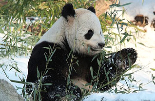
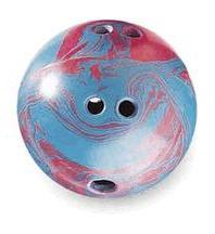
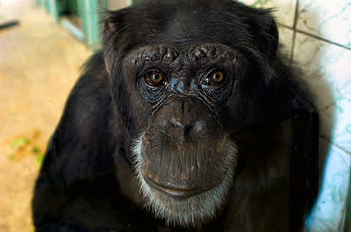
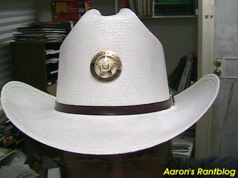
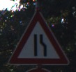
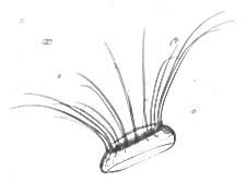
We choose 10 image classification tasks from very diverse domains including objects, hand-written digit and characters, pedestrians, sketches, traffic signs, planktons and house numbers. The dataset statistics are summarized in Table 1 and a few example images are given in Table 3.
In more detail, Animals with Attributes (AwA) [29] contains 30475 images of 50 animal species. While the dataset is introduced for zero-shot learning, it provides class labels for each image. Caltech-256 [14] is a standard object classification benchmark that consists of 256 object categories and an additional background class. CIFAR10 [26] consists of 60000 colour object classes in 10 classes. Daimler Mono Pedestrian Classification Benchmark [39] contains a collection of pedestrian and non-pedestrian images. Pedestrians are cropped and resized to pixels. The German Traffic Sign Recognition (GTSR) Benchmark [49] contains cropped images of 43 traffic signs. Sizes of the traffic signs vary between and pixels. MNIST [30] contains 70000 handwritten digits which are centred in images. Omniglot [28] consists of 1623 different handwritten characters from 50 different alphabets. The dataset is originally designed for one shot learning. Instead we include all the character categories in train and test time. Plankton imagery data [8] is a classification benchmark that contains 30336 images of various organisms ranging from the smallest single-celled protists to copepods, larval fish, and larger jellies. Human Sketch dataset [12] contains 20000 human sketches of every day objects such as “book”, “car”, “house”, “sun”. The Street View House Numbers (SVHN) [40] is a real-world digit recognition dataset with around 70,000 images which are centred around a single character and resized into pixels.
As the majority of datasets differ in terms of image resolutions and characteristics, images are resized to pixels, greyscale ones are converted into RGB by setting the three channels to the same value. Though it would be possible to maintain the images in the original resolution, using a single scale simplifies the network design. Each dataset is also whitened, by subtracting its mean and dividing it by its standard deviation per channel. For the datasets that do not have a fixed train and test splits, we use to ratio for train and test data respectively.
Architectures.
We choose to use the state-of-the-art Residual Networks [18] due to their remarkable capacity and performance. More specifically, for this experiment we select the ResNet-38 model. This network has a stack of 4 residual units with convolutions for each feature map size () and with number of filters respectively. The network ends with a global average pooling layer and a fully connected layer followed by softmax for classification. As the majority of the datasets have a different number of classes, we use a dataset-specific fully connected layer in our experiments unless otherwise stated.
As explained in section 3.3, datasets are balanced by sampling batches from different ones in a round-robin fashion during training. We follow the same data augmentation strategy in [18], the size whitened image is padded with 8 pixels on all sides and a patch randomly sampled from the padded image or its horizontal flip. Note that as MNIST, Omniglot and SVHN contain digits and characters, we do not augment flipped images from these datasets. The networks are trained using stochastic gradient descent with momentum. The learning range is set to 0.1 and gradually reduced to 0.0001 after a short warm-up training with a learning rate of 0.01 as in [18]. The weight decay and momentum are set to 0.9 and 0.0001 respectively. In test time, we use only the central crop of images and report percentages of top-1 error rate.
Next, we experiment with sharing features up to different depths in the architectures. To this end, the ResNet-38 model is modified to have a branch for each task , stemming from a common trunk .
Baseline: no sharing.
As a baseline, a different ResNet-38 model (i.e. ) is trained from scratch for each dataset until convergence (25k iterations are sufficient) using a batch size of 128 images and BN. Although our focus is not obtaining state-of-the-art results but demonstrating the effectiveness of sharing a representation among different domains, the chosen CNN provides a good speed and performance trade-off and achieves comparable results to state-of-the-art methods (see Table 3). The much deeper ResNet-1001 [18] obtains error rate in CIFAR-10 (compared to our ), DropConnect [56] with a heavier multi-column network obtains in MNIST (compared to our ) and Lee et al. [31] report (compared to our ) in SVHN by using more sophisticated pooling mechanisms. While the network yields relatively low error rates in the majority of the datasets, the absolute performance is less good in AwA and Caltech256. However, this is inline with the results reported in the literature, where good performance on such datasets was shown to require pre-training on a very large dataset such as ImageNet [11, 59]. In short, this validates our ResNet-38 baseine as a good and representative architecture.
| Sharing | AwA | Caltech | CIFAR10 | Daimler | GTSR | MNIST | Omniglot | Plankton | Sketches | SVHN | mean |
|---|---|---|---|---|---|---|---|---|---|---|---|
| no sharing | 77.9 | 85.1 | 9.4 | 10.4 | 4.2 | 0.34 | 13 | 25.7 | 31.1 | 3.7 | 26.1 |
| deep | 73.7 | 82.6 | 11.7 | 5.2 | 3.5 | 0.38 | 13.1 | 24.9 | 30.8 | 4.1 | 25.0 |
| partial (block 1-3) | 76.6 | 84.0 | 12.4 | 7.0 | 4.0 | 0.29 | 13.8 | 26.2 | 33.1 | 4.4 | 26.2 |
| partial (block 2-4) | 76.6 | 84.0 | 9.9 | 7.7 | 3.3 | 0.49 | 12.1 | 25.3 | 30.7 | 3.5 | 25.3 |
| deep ( params) | 74.0 | 81.7 | 9.1 | 4.2 | 4.1 | 0.43 | 12.3 | 25.8 | 29.1 | 3.5 | 24.4 |
| deep ( params) | 73.1 | 81.5 | 7.2 | 4.1 | 3.5 | 0.35 | 11.8 | 25 | 27.6 | 3.5 | 23.8 |
Full sharing.
Next, we consider the opposite of no sharing and share all the parameters of the network (i.e. ). A common belief is that only the relatively shallow layers of a CNN are shareable, whereas deeper ones are more domain-specific [32]. Full sharing challenges this notion.
In this experiment, ResNet-38 is configured with BN with domain-specific scaling parameters and moments . A single CNN is trained on three domains, CIFAR, MNIST, and SVHN, because such domains happens to contain exactly 10 classes each. Although CIFAR objects and MNIST/SVHN digits have nothing in common, we randomly pair digits with objects. This allows to share all filter parameters, including the final classification layer, realising full sharing.
As shown in Table 2, evaluated on the different datasets, the performance of this network is nearly the same as learning three independent models. This surprising result means that the model has sufficient capacity to learn classifiers that respond strongly either to a digit in MNIST or SVHN, or to an object in CIFAR, essentially learning an or operator. The question then is whether combining more problems together can eventually exceed the capacity of the network.
Deep sharing.
Next, we experiment with sharing all layers except the last one, which performs classification. In this case, therefore, is a single convolutional layer and contains the rest of the network, including all but the last fully connected layer. This setup is similar to full sharing, but allows to combine classification tasks even when these do not have an equal number of classes.
The results in Table 3 and Table 2 show that the shared CNN performs better than training domain-specific networks. Remarkably, this is true for all the tasks, and reduces the average error rate by . Remarkably, this improvement is obtained while reducing the overall number of parameters by a factor of 10.
Partial sharing.
Here, we investigate whether there can be a benefit in specializing at least part of the shared model for individual tasks. We test two settings. In the first setting, the network has dataset-specific parameters in the shallower block (i.e. the first stack of 4 residual units) — this should be beneficial to compensate for different low-level statistics in the domains. In the second setting, instead, the network specializes the last block— this should be beneficial in order to capture different higher-level concepts in for different tasks. Interestingly, the results in Table 3 show that deep sharing is, for this choice of datasets and model, the best configuration. Specializing the last block is only marginally worse () and better () than specializing the first block. This may indicate that high-level specialization is preferable.
Network capacity.
Experiments so far suggested that the model has sufficient capacity to accommodate all the tasks, despite their significant diversity. In fact, ten individual networks perform worse than a single, shared one. Next, we increase the capacity of the model, but we keep sharing all such parameters between tasks. In order to do so, we increase the number of convolutional filters twice () and four times (), which increases the number of parameters 4 and 16 times. Differently from learning 10 independent networks, this setup allows the model to better use the added capacity to accommodate the different tasks, reducing the mean error rate by and points, respectively. The fact that joint training can exploit the added capacity better suggests that the different domains overlap synergistically, despite their apparent differences.
Normalization strategies.
So far, we have shown that learning a single CNN for the 10 domains is not only possible, but in fact preferable to learining individual models. However, this CNN used a specific normalization strategy, BN, as well as domain-specific scaling parameters and moments .
In Table 4 we examine the importance of these design decisions. First, we note that BN with domain-agnostic scaling and moments performs very poorly on the test set, comparable to random chance, clearly due to its inability to compensate for the large variance among the different domains. If BN is applied at test time (BN+), such that moments are computed on the fly but domain-agnostic scaling is still used, results are better but still poor (). Domain-agnostic scaling works well as long as at least the moments are domain-specific (). However, the best combination is to use domain-specific moments and scalings ().
In contrast to BN, IN, which normalizes images individually, works just as well with domain-specific and domain-agnostic scaling. The price to pay is a drop in performance compared to BN with domain-specific parameters. However, this strategy has a significant practical advantage: IN with domain-agnostic scaling effectively uses only a single set of parameters, including all filter weights and scaling factors, for all domains. This suggest that such a representation may be applicable to novel domain without requiring any domain-specific tuning of the normalization parameters at all.
| normalization | mean error | ||
|---|---|---|---|
| BN | universal | universal | – |
| BN+ | universal | – | 46.3 |
| BN | universal | domain | 27.3 |
| BN | domain | domain | 25 |
| IN | universal | – | 30.2 |
| IN | domain | – | 30.4 |
4.2 Large datasets
Data.
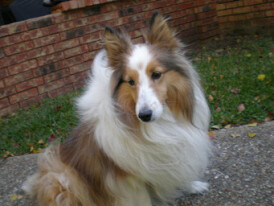
In this part, we consider three large scale computer vision tasks: object classification in ImageNet [46], face identification in VGG-Face [42], and word classification in Synth90k [22] dataset (Table 5). ImageNet contains 1000 object categories and 1.2 million images. VGG-Face dataset consists of 2.6 million face images of 2622 different people which are centered and resized into a fixed height of 128 pixels and a variable width. The Synth90k dataset contains approximately 9 million synthetic images for a 90k word lexicon which are generated with a fixed height of 32 pixels and variable width. We show example images from these datasets in Table 4.
 |
 |
|
 |
 |
|
| ImageNet | VGG-Face | Synth90k |
Implementation details.
ImageNet images are resized to pixels on their shortest side and maintaining the original aspect ratio. During training, random , and patches are cropped from ImageNet, VGG-Face and Synth90k respectively. As different input sizes lead to different feature map sizes at the last convolutional layer (a map for ImageNet down to a tiny map for the smallest Synth90k images – see below), we share the convolutional feature maps among the three tasks but use domain-specific fully connected layers. In training, we augment the data by randomly cropping, flipping and varying aspect ratio with the exception that we do not flip the images from Synth90k as they contain words. At test time, we only use a single center crop and report top1-error rates. The best normalization strategy (BN with domain specific scaling) identified in 4.1 is used.
Results.
We conduct two experiments. In the first one, a network is trained simultaneously on the ImageNet and VGG-Face datasets, with a significant difference in content as well as resolution between domains. We use an AlexNet model [27], adapt the dimensionality of the first fully connected layer (fc6) for the VGG-Face dataset, and train the networks from scratch. For this setting, the baseline is obtained by training two individual networks without any parameter sharing, obtaining and top-1 error rates on the ImageNet and VGG-Face respectively (see Table 5 — this is the same as published results). Sharing the convolutional weights between these tasks achieve comparable performance (there is a marginal drop of accuracy), illustrating once more the high degree of shareability of such representations.
In the second setting, we push the envelope by adding the Synth90k dataset which contains synthetically generated words for 90k different word classes. For this experiment, we use the higher-capacity model VGG-M-128 from [5]. This model has only 128 filters in the second to last fully connected layer (fc7), instead of 4096. As the Synth90k dataset contains 90k classes, having a small 128-dimensional bottleneck is necessary in order to maintain the size of the 90k classes classifier matrix (which is ) reasonable. Since Synth90k images are much smaller than the other two datasets, the last downsampling layer (pool5) is not used for this domain.
Without parameter sharing, this network performs similarly to AlexNet (due to the bottleneck which partially offsets the higher capacity). As before, the convolutional layer parameters are shared, and the fully-connected layers parameters are not. The results (see the bottom row in Table 5) show that the capacity of the model is pushed to its limit. Performance on ImageNet and VGG-Face is still very good, with a minor hit of 2-3%, but there is a larger drop for Synth90k ( error). Note that the total number of parameters in the joint network is a third of the sum of the individual network parameters. In order to have a fair comparison, we evaluate the performance of three independent models with a third of the parameters each (see the row in Table 5). We show that the jointly trained model performs dramatically better than the individual models, despite the fact that the total number of parameters is the same.
| ImageNet | VGG-Face | Synth90k | |
| No sharing | 40.5 | 25.7 | - |
| Deep (conv1-5) | 41.8 | 26.3 | - |
| No sharing | 40.8 | 25.7 | 12.1 |
| No sharing () | 49.2 | 57.1 | 39.0 |
| Deep (conv1-5) | 43.0 | 27.8 | 26.8 |
5 Conclusions
As machine vision consolidates, the challenge of developing universal models that, similarly to human vision, can be trained once and solve a large variety of problems, will come into focus. A component of such systems will be universal representations, i.e. feature extractors that work well for all visual domains, despite the significant diversity of the latter.
In this paper, we have shown that standard deep neural networks are already capable of learning very different visual domains together, with a high degree of information sharing. However, we have also shown that successful sharing requires tuning certain normalization parameters in the networks, preferably by using domain-specific scaling factors, in order to compensate for inter-domain statistical shifts. Alternatively, techniques such as instance normalization can compensate for such difference on the fly, in a domain-agnostic manner.
Overall, our findings are very encouraging. Universal representations seem to be within the grasp of current technology, at least for a wide array of real-world problems. In fact, while our most convincing results have been obtained for smaller datasets, we believe that larger problems can be addressed just as successfully by a moderate increase of model capacity and other refinements to the technology.
References
- [1] J. Atkinson. The Developing Visual Brain. Oxford University Press, 2002.
- [2] J. L. Ba, J. R. Kiros, and G. E. Hinton. Layer normalization. In arXiv, 2016.
- [3] H. Bilen and A. Vedaldi. Integrated perception with recurrent multi-task neural networks. In Proc. NIPS, 2016.
- [4] R. Caruana. Multitask learning. Machine Learning, 28, 1997.
- [5] K. Chatfield, K. Simonyan, A. Vedaldi, and A. Zisserman. Return of the devil in the details: Delving deep into convolutional nets. In Proc. BMVC, 2014.
- [6] T. Chen, I. Goodfellow, and J. Shlens. Net2net: Accelerating learning via knowledge transfer. arXiv preprint arXiv:1511.05641, 2015.
- [7] M. Cimpoi, S. Maji, and A. Vedaldi. Deep convolutional filter banks for texture recognition and segmentation. CoRR, abs/1411.6836, 2014.
- [8] R. K. Cowen, S. Sponaugle, K. Robinson, and J. Luo. Planktonset 1.0: Plankton imagery data collected from f.g. walton smith in straits of florida from 2014-06-03 to 2014-06-06 and used in the 2015 national data science bowl. NODC Accession 127422, 2015.
- [9] J. Dai, K. He, and J. Sun. Instance-aware semantic segmentation via multi-task network cascades. In Proc. CVPR, 2016.
- [10] J. Dai, K. He, and J. Sun. Instance-aware semantic segmentation via multi-task network cascades. In Proc. CVPR, 2016.
- [11] J. Donahue, Y. Jia, O. Vinyals, J. Hoffman, N. Zhang, E. Tzeng, and T. Darrell. Decaf: A deep convolutional activation feature for generic visual recognition. CoRR, abs/1310.1531, 2013.
- [12] M. Eitz, J. Hays, and M. Alexa. How do humans sketch objects? ACM Trans. Graph. (Proc. SIGGRAPH), 31(4):44:1–44:10, 2012.
- [13] Y. Ganin and V. Lempitsky. Unsupervised domain adaptation by backpropagation. Proc. ICML, 2015.
- [14] G. Griffin, A. Holub, and P. Perona. Caltech-256 object category dataset. 2007.
- [15] A. Gupta, A. Vedaldi, and A. Zisserman. Synthetic data for text localisation in natural images. Proc. CVPR, 2016.
- [16] K. He, X. Zhang, S. Ren, and J. Sun. Delving deep into rectifiers: Surpassing human-level performance on imagenet classification. CoRR, (arXiv:1502.01852v1), 2015.
- [17] K. He, X. Zhang, S. Ren, and J. Sun. Deep residual learning for image recognition. In Proc. CVPR, 2016.
- [18] K. He, X. Zhang, S. Ren, and J. Sun. Identity mappings in deep residual networks. arXiv preprint arXiv:1603.05027, 2016.
- [19] G. Hinton, O. Vinyals, and J. Dean. Distilling the knowledge in a neural network. arXiv preprint arXiv:1503.02531, 2015.
- [20] Y. Hong, R. Arandjelović, and A. Zisserman. Faces in places: Compound query retrieval. In Proc. BMVC, 2016.
- [21] S. Ioffe and C. Szegedy. Batch normalization: Accelerating deep network training by reducing internal covariate shift. CoRR, 2015.
- [22] M. Jaderberg, K. Simonyan, A. Vedaldi, and A. Zisserman. Synthetic data and artificial neural networks for natural scene text recognition. In NIPS Deep Learning Workshop, 2014.
- [23] M. Jaderberg, K. Simonyan, A. Vedaldi, and A. Zisserman. Reading text in the wild with convolutional neural networks. IJCV, 116(1):1–20, 2016.
- [24] A. Jamaludin, T. Kadir, and A. Zisserman. Spinenet: Automatically pinpointing classification evidence in spinal mris. In Proc. MICCAI, 2016.
- [25] I. Kokkinos. Ubernet: Training auniversal’convolutional neural network for low-, mid-, and high-level vision using diverse datasets and limited memory. arXiv preprint arXiv:1609.02132, 2016.
- [26] A. Krizhevsky and G. Hinton. Learning multiple layers of features from tiny images. 2009.
- [27] A. Krizhevsky, I. Sutskever, and G. E. Hinton. Imagenet classification with deep convolutional neural networks. In Proc. NIPS, 2012.
- [28] B. M. Lake, R. Salakhutdinov, and J. B. Tenenbaum. Human-level concept learning through probabilistic program induction. Science, 350(6266):1332–1338, 2015.
- [29] C. H. Lampert, H. Nickisch, and S. Harmeling. Learning to detect unseen object classes by between-class attribute transfer. In Proc. CVPR, pages 951–958, 2009.
- [30] Y. LeCun, C. Cortes, and C. J. Burges. The mnist database of handwritten digits, 1998.
- [31] C.-Y. Lee, P. W. Gallagher, and Z. Tu. Generalizing pooling functions in convolutional neural networks: Mixed, gated, and tree. In International Conference on Artificial Intelligence and Statistics, 2016.
- [32] K. Lenc and A. Vedaldi. Understanding image representations by measuring their equivariance and equivalence. In Proc. CVPR, 2015.
- [33] Z. Li and D. Hoiem. Learning without forgetting. In Proc. ECCV, pages 614–629. Springer, 2016.
- [34] T.-Y. Lin, A. RoyChowdhury, and S. Maji. Bilinear cnn models for fine-grained visual recognition. In Proc. ICCV, 2015.
- [35] W. Liu, D. Anguelov, D. Erhan, C. Szegedy, S. Reed, C.-Y. Fu, and A. C. Berg. Ssd: Single shot multibox detector. In Proc. ECCV, 2016.
- [36] M. Long and J. Wang. Learning transferable features with deep adaptation networks. CoRR, abs/1502.02791, 1:2, 2015.
- [37] I. Misra, A. Shrivastava, A. Gupta, and M. Hebert. Cross-stitch networks for multi-task learning. Proc. CVPR, 2016.
- [38] T. Mitchell. Never-ending learning. Technical report, DTIC Document, 2010.
- [39] S. Munder and D. M. Gavrila. An experimental study on pedestrian classification. PAMI, 28(11):1863–1868, 2006.
- [40] Y. Netzer, T. Wang, A. Coates, A. Bissacco, B. Wu, and A. Y. Ng. Reading digits in natural images with unsupervised feature learning. 2011.
- [41] M. Oquab, L. Bottou, I. Laptev, and J. Sivic. Learning and Transferring Mid-Level Image Representations using Convolutional Neural Networks. In Proc. CVPR, 2014.
- [42] O. M. Parkhi, A. Vedaldi, and A. Zisserman. Deep face recognition. In British Machine Vision Conference, 2015.
- [43] A. S. Razavian, H. Azizpour, J. Sullivan, and S. Carlsson. Cnn features off-the-shelf: an astounding baseline for recognition. In Proc. CORR, 2014.
- [44] S. Ren, K. He, R. Girshick, and J. Sun. Faster r-cnn: Towards real-time object detection with region proposal networks. In arXiv:1506.01497, 2015.
- [45] A. Romero, N. Ballas, S. E. Kahou, A. Chassang, C. Gatta, and Y. Bengio. Fitnets: Hints for thin deep nets. arXiv preprint arXiv:1412.6550, 2014.
- [46] O. Russakovsky, J. Deng, H. Su, J. Krause, S. Satheesh, S. Ma, Z. Huang, A. Karpathy, A. Khosla, M. Bernstein, A. C. Berg, and L. Fei-Fei. Imagenet large scale visual recognition challenge, 2014.
- [47] F. Schroff, D. Kalenichenko, and J. Philbin. Facenet: A unified embedding for face recognition and clustering. In arXiv, volume arXiv:1503.03832v1, 2015.
- [48] D. L. Silver, Q. Yang, and L. Li. Lifelong machine learning systems: Beyond learning algorithms. In AAAI Spring Symposium: Lifelong Machine Learning, pages 49–55. Citeseer, 2013.
- [49] J. Stallkamp, M. Schlipsing, J. Salmen, and C. Igel. Man vs. computer: Benchmarking machine learning algorithms for traffic sign recognition. Neural Networks, (0):–, 2012.
- [50] C. Szegedy, V. Vanhoucke, S. Ioffe, and J. Shlens. Rethinking the inception architecture for computer vision. In Proc. CVPR, 2016.
- [51] Y. Taigman, M. Yang, M. A. Ranzato, and L. Wolf. Deepface: Closing the gap to human-level performance in face verification. In Proc. CVPR, 2014.
- [52] A. V. Terekhov, G. Montone, and J. K. O’Regan. Knowledge transfer in deep block-modular neural networks. In Conference on Biomimetic and Biohybrid Systems, pages 268–279. Springer, 2015.
- [53] S. Thrun. Lifelong learning algorithms. In Learning to learn, pages 181–209. Springer, 1998.
- [54] E. Tzeng, J. Hoffman, T. Darrell, and K. Saenko. Simultaneous deep transfer across domains and tasks. In Proc. CVPR, pages 4068–4076, 2015.
- [55] D. Ulyanov, A. Vedaldi, and V. S. Lempitsky. Instance normalization: The missing ingredient for fast stylization. CoRR, abs/1607.08022, 2016.
- [56] L. Wan, M. Zeiler, S. Zhang, Y. L. Cun, and R. Fergus. Regularization of neural networks using dropconnect. In Proceedings of the 30th International Conference on Machine Learning (ICML-13), pages 1058–1066, 2013.
- [57] X. Wang, D. Fouhey, and A. Gupta. Designing deep networks for surface normal estimation. In Proceedings of the IEEE Conference on Computer Vision and Pattern Recognition, pages 539–547, 2015.
- [58] J. Yosinski, J. Clune, Y. Bengio, and H. Lipson. How transferable are features in deep neural networks? Proc. NIPS, 2014.
- [59] M. D. Zeiler and R. Fergus. Visualizing and understanding convolutional networks. In Proc. ECCV, 2014.
- [60] T. Zhang, B. Ghanem, S. Liu, and N. Ahuja. Robust visual tracking via structured multi-task sparse learning. IJCV, 101(2):367–383, 2013.
- [61] Z. Zhang, P. Luo, C. C. Loy, and X. Tang. Facial landmark detection by deep multi-task learning. In Proc. ECCV, 2014.