The Molecular Cloud Lifecycle I:
Constraining H₂ formation and dissociation rates with observations

Abstract

Molecular clouds (MCs) are the birthplaces of new stars in galaxies. A key component of MCs are photodissociation regions (PDRs), where far-ultraviolet radiation plays a crucial role in determining the gas’s physical and chemical state. Traditional PDR models assume chemical steady state (CSS), where the rates of H₂ formation and photodissociation are balanced. However, real MCs are dynamic and can be out of CSS. In this study, we demonstrate that combining H₂ emission lines observed in the far-ultraviolet or infrared with column density observations can be used to derive the rates of H₂ formation and photodissociation. We derive analytical formulae that relate these rates to observable quantities, which we validate using synthetic H₂ line emission maps derived from the SILCC-Zoom hydrodynamical simulation. Our method estimates integrated H₂ formation and dissociation rates to within 29% accuracy. Our simulations cover a wide dynamic range in H₂ formation and photodissociation rates, showing significant deviations from CSS, with 74% of the MC’s mass deviating from CSS by a factor greater than 2. Our analytical formulae can effectively distinguish between regions in and out of CSS. When applied to actual H₂ line observations, our method can assess the chemical state of MCs, providing insights into their evolutionary stages and lifetimes.

1 Introduction

Molecular hydrogen (H₂), the most abundant molecule in the universe, plays a crucial role in the lifecycle of baryons throughout cosmic history (Galli & Palla, 1998; McKee & Ostriker, 2007; Tacconi et al., 2020). It acts as a vital cooling agent in the early universe (Haiman et al., 1996; Bromm et al., 2001; Omukai, 2000; Barkana & Loeb, 2001; Bialy & Sternberg, 2019), triggers rich chemistry in the interstellar medium (ISM) (Herbst & Klemperer, 1973; Tielens, 2013; van Dishoeck et al., 2013; Bialy & Sternberg, 2015), and correlates with the star formation rate in present-day galaxies (Bigiel et al., 2008; Leroy et al., 2008; Schruba et al., 2011).

H₂ is predominantly found in molecular clouds (MCs) and is excited by far-UV (FUV) radiation within the Lyman-Werner (LW) band ($h\nu=11.2-13.6$ eV). LW photons excite the electronic $B^{1}\Sigma^{+}_{u}$ and $C^{1}\Pi_{u}$ states of H₂. These excited states can then radiatively decay through two pathways: (a) to the rovibrational continuum, leading to H₂ dissociation and the emission of FUV continuum radiation; or (b) to a bound (rovibrationally excited) level in the ground electronic state ($X^{1}\Sigma^{+}_{g}$), accompanied by FUV line emission (Field et al. 1966; Stecher & Williams 1967; Dalgarno et al. 1970; Sternberg 1989, hereafter S89). The rovibrationally excited H₂ molecules continue to cascade down the rovibrational ladder, emitting infrared (IR) lines (Black & van Dishoeck, 1987; Sternberg, 1988; Luhman et al., 1994; Neufeld & Spaans, 1996).

In this study, we focus on photodissociation regions (PDRs), where radiative processes dominate molecular excitation and dissociation (Tielens & Hollenbach, 1985; Hollenbach & Tielens, 1999; Le Petit et al., 2006; Röllig et al., 2007; Bisbas et al., 2021; Röllig & Ossenkopf-Okada, 2022; Pound & Wolfire, 2023). This includes gas in the vicinity of massive stars (e.g., the Orion nebula) and MCs embedded in the ambient interstellar radiation field, as long as the dust visual extinction is not too large. In contrast, in cloud cores, LW radiation is strongly attenuated due to H₂ self-shielding and dust absorption. In these well-shielded regions, H₂ excitation and dissociation are driven by deep-penetrating cosmic rays or X-rays (Maloney et al., 1996; Dalgarno, 2006; Wolfire et al., 2022; Bialy, 2020). However, even for MCs exposed only to the ambient interstellar radiation field, photoprocesses dominate H₂ dissociation, excitation, and line emission up to gas column densities of $N\approx 10^{22}$ cm^-2 (Sternberg et al., 2024; Padovani et al., 2024, see also §5.2 of this paper, and the Appendix).

Traditional PDR models assume that the total formation and destruction rates of H₂ (and other molecules) balance each other, i.e., that the system is in chemical steady state (CSS). This allows efficient characterization of MCs since the abundance and emission spectrum of H₂ are time-independent and depend only on physical conditions such as the FUV radiation field intensity, gas density, and gas metallicity. For example, the CSS assumption allows the derivation of useful analytic formulae describing: (a) the atomic-to-molecular transition point (Bialy & Sternberg, 2016), (b) the total HI column density (Krumholz et al., 2008, 2009; Sternberg et al., 2014; Bialy et al., 2017), and (c) the total intensity of H₂ line emission (S89). This analytic framework has been utilized in the analysis of observations in various Galactic and extragalactic PDRs (e.g. Bialy et al., 2015; Schruba et al., 2018; Ranjan et al., 2018; Noterdaeme et al., 2019; Syed et al., 2022).

However, in practice, the assumption of CSS may be problematic. MCs are dynamic entities. They form in regions of converging flows (e.g., in gas that is infalling onto galactic spiral arms, collisions of expanding supernova shells, etc.), where gas may be compressed to high densities (Koyama & Inutsuka, 2000; Hartmann et al., 2002; Ntormousi et al., 2011; Dawson, 2013; Bialy et al., 2021). Once gravitational collapse is initiated, newly formed stars begin to disperse the gas through various stellar feedback processes: ionizing radiation, stellar winds, jets, and supernova explosions (McKee & Ostriker, 1977; Faucher-Giguère et al., 2013; Hopkins et al., 2020; Orr et al., 2022; Ostriker & Kim, 2022; Chevance et al., 2023). These dynamical processes can occur on short timescales compared to the time required for the gas to achieve CSS, and thus MCs may be out of CSS (Glover & Mac Low, 2007; Krumholz, 2012; Richings et al., 2014; Hu et al., 2016; Valdivia et al., 2016; Seifried et al., 2017, 2022).

This raises an important question: Can we determine from observations whether a given MC is in or out CSS?
In this paper, we illustrate how combining the total intensity in H₂ line emission with the total gas and HI column densities along the line of sight (LOS), allows us to obtain reliable estimates for the column-integrated rates of H₂ photodissociation and formation. This enables us to assess whether a CSS is maintained.

The question of whether a MC is in or out of CSS has important implications for MCs’ lifetimes and evolution. If the gas in a MC is found to be far from CSS it implies that the MC has either been recently replenished with “fresh” gas or has lost gas via evaporation, over a timescale that is short compared to the chemical time (i.e., Eq. 5 below; see also Jeffreson et al. 2024). In a second paper in this series (Burkhart et al., 2024), we explore in more detail the time evolution of MCs, the evolution of the H₂ formation and photodissociation rates in MCs, and their relationship to the star formation rate.

The structure of this paper is as follows: in §2, we provide the fundamental theoretical framework. We derive the key analytical equations, namely Eqs. (9, 12), which elucidate how an observer can employ H₂ line emission intensities and column density maps to calculate integrated H₂ formation and dissociation rates along the line of sight. In §3 we present the magnetohydrodynamical simulations and the numerical procedure for producing H₂ line intensity maps. We use these maps to test our analytic theory. In §4 we present our results, relating the state of the gas in the simulation and the H₂ formation and dissociation rates in various cloud regions to the observables. We follow up with a discussion and conclusions in §5 and §6.

2 Theoretical Model

2.1 H₂ formation and dissociation

For typical ISM conditions, H₂ formation is dominated by dust catalysis (Wakelam et al., 2017). The destruction of H₂ is dominated by photodissociation. The net change in number of H₂ molecules per unit time and volume is

$$\frac{\mathrm{d}n({\rm H_{2}})}{\mathrm{d}t}=j_{F}-j_{D}$$ (1)

where

$$j_{F}\equiv n({\rm H})nR\;,\;\;j_{D}\equiv n({\rm H_{2}})D\ ,$$ (2)

are the volumetric H₂ formation and dissociation rates (cm^-3 s^-1). Here, $R$ (cm³ s^-1) is the H₂ formation rate coefficient, $D$ (s^-1) is the local photodissociation rate, which may be significantly attenuated due to H₂ self-shielding and dust absorption (see below), $n({\rm H})$ and $n({\rm H_{2}})$, are the H and H₂ number densities, respectively, and $n$ is the total hydrogen nucleon density (cm^-3). In Eq. (2) and throughout our analytic model we consider only H₂ photodissociation and neglect additional H₂ destruction via cosmic-rays. This assumption is justified in §5.2 and in the Appendix.

In this work, we use the “SImulating the Life-Cycle of molecular Clouds” (SILCC)-Zoom (Seifried et al., 2017) simulation suite to produce synthetic maps of H₂ line emission (as described below). In line with the SILCC simulation suite, we adopt an H₂ formation rate coefficient

$$R=3\times 10^{-17}T_{2}^{1/2}Sf_{a}Z_{d}^{\prime}\ {\rm cm^{3}\ s^{-1}}\ ,$$ (3)

where $S=[1+0.4(T_{2}+T_{d,2})^{0.5}+0.2T_{2}+0.08T_{2}^{2}]^{-1}$ is the sticking coefficient, $f_{a}=[1+10^{4}\mathrm{e}^{-600{\rm K}/T_{d}}]^{-1}$ is the fraction of H atoms that enter the potential wells on the dust grain before evaporating and thus ultimately combine to form H₂ molecules (Hollenbach & McKee, 1979), $Z_{d}^{\prime}$ is the dust-to-gas ratio relative to the Solar neighborhood ISM, $T$ and $T_{d}$ are the gas and dust temperatures, and $T_{2}\equiv T/(10^{2}{\rm K})$. The H₂ photodissociation rate is given by

$$D=\chi D_{0}f_{\rm H_{2},shield}f_{\rm dust}\ ,$$ (4)

where $\chi=F_{\rm FUV}/F_{0}$ is the flux of the incident FUV radiation field on the cloud relative to the typical Solar neighborhood value, $F_{0}=2.7\times 10^{-3}$ erg cm^-2 s^-1 (Draine, 1978; Bialy, 2020), and $D_{0}=5.8\times 10^{-11}$ s^-1 is the free-space photodissociation rate in the absence of shielding (Sternberg et al., 2014). The functions $f_{\rm H_{2},shield}$ and $f_{\rm dust}$ account for LW attenuation by H₂ lines (self-shielding) and by dust absorption (see §3.1 and the discussion after Eqs. A1-A2 for more details).

In CSS $j_{F}=j_{D}$, and at any cloud position, the H₂-to-H ratio is then given by $n({\rm H_{2}})/n({\rm H})=Rn/D$. If $j_{F}\neq j_{D}$ the system is out of CSS: for $j_{F}>j_{D}$, there is net H₂ formation and the H₂ mass grows with time, whereas if $j_{F}<j_{D}$ the H₂ mass decreases with time.

For a given value of $D$, $R$ and $n$, the timescale to reach CSS is

$$t_{\rm chem}=\frac{1}{2nR+D}\ ,$$ (5)

This follows from Eq. (1-2) (see Bialy et al., 2017, for a derivation). Near cloud boundaries, where there is no LW attenuation, $D=\chi D_{0}\gg 2Rn$. Under these conditions, the chemical time is very short: $t_{\rm chem}=1/(\chi D_{0})=550/\chi$ years. In deep cloud interiors, where radiation is significantly attenuated by dust and line absorption, $D\ll 2Rn$. In this regime, the chemical time equals the H₂ formation time:

$$t_{\rm chem}\rightarrow t_{\rm H_{2},form}\equiv\frac{1}{2Rn}\approx 9\left(\frac{1}{Z_{d}^{\prime}n_{2}}\right)\ {\rm Myr}\ ,$$ (6)

where for the numerical evaluation we used Eq. (3) with typical CNM conditions, $T=100$ K, $T_{d}\ll T$, and defined $n_{2}\equiv n/(100\ {\rm cm^{-3}})$. Thus, cloud envelopes, characterized by short chemical timescales, tend to be in CSS, while cloud interiors, which exhibit long chemical timescales, are prone to deviate from CSS.

Hereafter we adopt typical solar-neighborhood values for the FUV radiation field intensity and the dust-to-gas ratio, $Z_{d}^{\prime}=1$, $\chi=1$.

2.2 Estimating H₂ formation-dissociation with observations

In this subsection, we discuss how we can use emission line observations to derive the H₂ formation and dissociation rates. As observations are probing integral quantities (integrated along the LOS) rather than volumetric quantities, we define the column-integrated H₂ formation and dissociation mass rates

$$\dot{\Sigma}_{F}^{\rm(true)} \equiv\bar{m}\int j_{F}\mathrm{d}s=\bar{m}\int n({\rm H})nR\mathrm{d}s$$ (7)

$$\dot{\Sigma}_{D}^{\rm(true)} \equiv\bar{m}\int j_{D}\mathrm{d}s=\bar{m}\int n({\rm H_{2}})D\mathrm{d}s\ ,$$

where $s$ is the coordinate along the LOS. The quantities $\dot{\Sigma}_{F}^{\rm(true)}$ and $\dot{\Sigma}_{D}^{\rm(true)}$ express the gas mass that is converted from atomic to molecular form and vise versa, per unit area and time ($M_{\odot}$ pc^-2 Myr^-1). We adopt a mean particle mass $\bar{m}=2m_{\rm H}\times 1.4=4.7\times 10^{-24}$ g, corresponding to the mass of an H₂ molecule, with the additional helium contribution assuming cosmic He abundance. We use the superscript “(true)” to stress that these are the true rates, as calculated by integrating the volumetric rates in our simulation. This is as opposed to the observationally-estimated rates (defined below), that are derived from observable quantities such as H₂ line intensities and column densities.

2.2.1 The H₂ photodissociation rate

As discussed in §1, H₂ photodissociation occurs via a two-step process in which first the electronic states of H₂ are photo-excited. The radiative decay to the rovibrational continuum of the ground electronic state leads to H₂ dissociation. The probability of dissociation per excitation is given by

$$p_{\rm diss}\equiv{D/P}\approx 0.15\ ,$$ (8)

where $P$ is the total H₂ photo-excitation rate (of all H₂ electronic states) (Abgrall et al., 1992; Draine & Bertoldi, 1996). In the remaining 85% of the cases, the H₂ decays to rovibrational bound states, producing FUV and subsequently IR line emission. In addition to line emission, H₂ electronic excitation also results in the emission of continuum FUV radiation (Dalgarno et al., 1970) which can also be observed and used to constrain the H₂ excitation and dissociation rates. In this paper, we focus on line emission, with our analytic and numerical analysis in §§§2-4 concentrating on FUV lines. We then generalize to IR lines in §5.

Since the process of H₂ photo-excitation results in both line emission and H₂ dissociation, the H₂ dissociation rate is proportional to the total intensity of the H₂ emission lines. As we show in the Appendix (Eq. A6), this relation is given by

$$\dot{\Sigma}_{D}^{\rm(obs)} =\frac{4\pi p_{\rm diss}\bar{m}}{1-p_{\rm diss}}\ \mathcal{I}_{\rm tot}\left(\frac{\tau_{\rm tot}}{1-\mathrm{e}^{-\tau_{\rm tot}}}\right)$$ (9)

$$=0.30\ \mathcal{I}_{5}\left(\frac{N_{21}}{1-\mathrm{e}^{-1.9N_{21}}}\right)\ {\rm M_{\odot}\ pc^{-2}\ Myr^{-1}}\ ,$$

where $\mathcal{I}_{\rm tot}$ is the total photon intensity summed over all the FUV emission lines (photons cm^-2 s^-1 str^-1), and $\tau_{\rm tot}=\sigma N$ is the dust optical depth at the LW band along the LOS, $\sigma$ is the dust absorption cross section per hydrogen nucleus, and $N$ is the column density of hydrogen nuclei along the LOS. In the last equality, we defined $\mathcal{I}_{\rm 5}\equiv\mathcal{I}_{\rm tot}/({10^{5}\ {\rm photons\ cm^{-2}\ s^{-1}\ sr^{-1}}})$, $N_{21}\equiv N/(10^{21}\ {\rm cm^{-2}})$, and used $\sigma=1.9\times 10^{-21}$ cm² (Sternberg et al., 2014), which is our fiducial value for $\sigma$ in this paper. We use the superscript (obs) to indicate that this expression approximates the true photodissociation rates, relying on integrated observable quantities rather than the detailed 3D density structure, and radiation geometry information (see Appendix).

The factor in parenthesis expresses the absorption of the emitted H₂ lines by intervening dust. This factor connects smoothly the optically thin and thick regimes. In the optically thin limit ($\tau_{\rm tot}\ll 1$) this factor approaches unity, and $\dot{\Sigma}_{D}^{\rm(obs)}\propto\mathcal{I}_{\rm tot}$. In this limit, the H₂ emission lines directly trace the integrated H₂ photodissociation rate. On the other hand, in the optically thick limit ($\tau_{\rm tot}>1$), the factor $\tau_{\rm tot}/(1-\mathrm{e}^{-\tau_{\rm tot}})\rightarrow\tau_{\rm tot}$, and the ratio $\dot{\Sigma}_{D}^{\rm(obs)}/\mathcal{I}_{\rm tot}$ grows linearly with $\tau_{\rm tot}$. In this limit, $\mathcal{I}_{\rm tot}$ traces only the outer part of the cloud, at an optical depth of $\approx 1$. While observed lines originate mainly from outer cloud envelopes, H₂ photodissociation can still occur deeper within clouds as FUV radiation penetrates through lower opacity regions in the patchy structure, not necessarily along the LOS.

For typical molecular clouds in our Galactic neighbourhood, $\tau_{\rm tot}\approx 1$ ($N_{21}\approx 0.5$), $\mathcal{I}_{5}\approx 0.3-0.6$, and the integrated H₂ photodissociation rate is $\approx 0.1$ M_☉ pc^-2 Myr^-1.

2.2.2 The H₂ formation rate

Since H₂ formation involves H atoms that interact on dust grains, the integrated formation rate may be derived from observations of the H I column density (via the 21 cm emission line). To see this, we first define the effective-mean $Rn$ factor,

$$\langle Rn\rangle_{\rm eff}\equiv\frac{\int(Rn)n({\rm H})\mathrm{d}s}{\int n({\rm H})\mathrm{d}s}\ .$$ (10)

Using this definition, we can rewrite Eq. (7) as

$$\dot{\Sigma}_{F}^{\rm(true)}=\bar{m}\langle Rn\rangle_{\rm eff}N({\rm H})\ ,$$ (11)

where $N({\rm H})$ is the H column density.

First, let us gain intuition by considering a simple case of a uniform density and temperature slab. In this case, Eq. (10) simplifies to $\langle Rn\rangle_{\rm eff}=Rn$. For typical cold neutral medium (CNM) conditions $n\approx 30$ cm^-3, $T=100$ K (Wolfire et al., 2003; Bialy & Sternberg, 2019). With Eq. (3) we get $Rn=3.4\times 10^{-16}$ s^-1. For a CNM column density of $5\times 10^{20}$ cm^-2 we get an integrated H₂ formation rate of $\approx 0.1~{}{\rm M_{\odot}\ pc^{-2}\ Myr^{-1}}$.

In practice, the gas density and temperature vary inside the cloud, and the value of $\langle Rn\rangle_{\rm eff}$ differs from one LOS to another. 3D dust maps offer insights into density structure (e.g., Leike et al. 2020; Zucker et al. 2021), but they lack the resolution to capture the critical HI-to-H₂ transition length. This transition, occurring over scales $\lesssim 1$ pc (Bialy et al., 2017), is crucial for studying the H-H$2$ balance and clouds’ chemical state. Due to this resolution limitation, we must rely on readily observable LOS-integrated quantities to estimate $\langle Rn\rangle{\rm eff}$. From a theoretical point of view, $\langle Rn\rangle_{\rm eff}$ is expected to correlate with the integrated gas column density $N$. This is because particles that are situated in large reservoirs of mass will typically have large integrated column density along the LOS (i.e., large $N$), while on the other hand these particles are situated in deeper gravitational potential wells leading to gas compression (i.e., higher $n$).

This correlation has been observed in various independent hydro simulations of the interstellar medium (i.e., the $A_{V}-n$ relation; Bisbas et al., 2019; Hu et al., 2021; Bisbas et al., 2021; Gaches et al., 2022). Using our SILCC-Zoom simulations, we find that $\langle Rn\rangle_{\rm eff}$ is well described by the powerlaw relation $\langle Rn\rangle_{\rm eff}=k_{0}N_{21}^{\alpha}$ with $k_{0}=2.0\times 10^{-16}$ s^-1 and $\alpha=1.3$. With this power law relation we get

$$\dot{\Sigma}_{F}^{\rm(obs)} =\bar{m}k_{0}N_{21}^{\alpha}N(\rm H)$$ (12)

$$=0.14\ f_{\rm H}N_{21}^{1+\alpha}\ {\rm M_{\sun}\ pc^{-2}\ Myr^{-1}}\ ,$$

where $\alpha=1.3$, and where we defined $f_{\rm H}\equiv N({\rm H})/N$.

Similarly to the case of $\dot{\Sigma}_{D}^{\rm(obs)}$, here, too, we use the superscript (obs) to emphasize that $\dot{\Sigma}_{F}^{\rm(obs)}$ is derived based on observed quantities only, and is an approximation to the true rate. In §4 we test the accuracy of these approximations using our hydro simulations.

2.2.3 The formation to photodissociation rate ratio

Combining Eqs. (9) and (12), we obtain the formation to dissociation rate ratio

$$\left(\frac{\dot{\Sigma}_{F}}{\dot{\Sigma}_{D}}\right)^{\rm(obs)} =\frac{k_{0}N_{21}^{\alpha}N({\rm H})}{4\pi\mathcal{I}_{\rm tot}(\frac{\tau_{\rm tot}}{1-\mathrm{e}^{-\tau_{\rm tot}}})}\frac{1-p_{\rm diss}}{p_{\rm diss}}\ ,$$ (13)

$$=0.47\ N_{21}^{\alpha}f_{\rm H}\left(1-\mathrm{e}^{-1.9N_{21}}\right)\mathcal{I}_{5}^{-1}\ .$$

If CSS holds, $\dot{\Sigma}_{F}/\dot{\Sigma}_{D}=1$. If $\dot{\Sigma}_{F}/\dot{\Sigma}_{D}>1$, then the gas along the LOS is not in CSS, and the H₂ column density increases with time at the expense of HI. If $\dot{\Sigma}_{F}/\dot{\Sigma}_{D}<1$, the H₂ column density decreases with time, and HI increases. Thus, given an observation of the gas HI and total column density and an H₂ emission spectrum, we can constrain the chemical state of the gas and whether it is in CSS, or not.

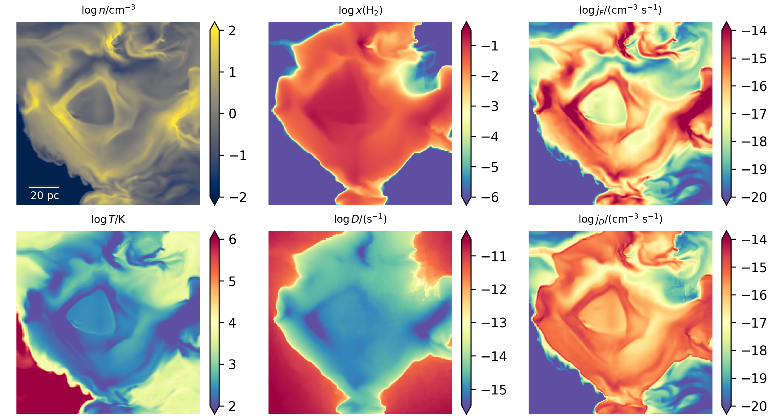
Figure 1: A 2D slice (xy plane) through the SILCC-Zoom simulation. The box size is $125{\rm pc}\times 125{\rm pc}$. The different panels show the gas density, the gas temperature, the H₂ abundance ($x({\rm H_{2}})\equiv n({\rm H_{2}})/n$), the H₂ photodissociation rate (Eq. 4), and the volumetric H₂ formation and photodissociation rates (Eq. 2). For an interactive figure, see sbialy.wixsite.com/astro/visuals.

Quantity	value
Simulation side length	$125$ pc
Resolution	$512^{3}$
Mean density	$3.3$ cm-3
Radiation field strength ($\chi$)	1
Total gas mass	$2.2\times 10^{5}\ M_{\odot}$
Fraction of gas out of CSS	41% (by volume)
	74% (by mass)

Table 1: The bottom two rows show our results for the fraction of cells out of CSS, where we define CSS as $0.5<(j_{F}/j_{D})<2$.

3 Numerical Method

3.1 Hydro Simulations

We generate synthetic maps of H₂ line emission, formation rate, and dissociation rate using the SILCC-Zoom simulations (Seifried et al., 2017). These are high-resolution zoom-in runs derived from the SILCC simulation suite (Walch et al., 2015; Girichidis et al., 2015). The SILCC simulation suite is a set of magnetohydrodynamical models of the chemical and thermal state of the ISM and the formation of stars in realistic galactic environments. The SILCC simulations have a stratified-box geometry. They include self-gravity as well as a background potential for the Galactic disk. Each simulation follows the thermal evolution of the gas and dust, including photoelectric heating by dust, cosmic-ray ionization heating, and radiative cooling through various atoms ions, and molecules. The chemistry of the ISM is modeled using an “on-the-fly” time-dependent network for hydrogen and carbon chemistry, tracking the evolution of the chemical abundances of free electrons, O, H⁺, H, H₂, C⁺, and CO. The simulation models H-H₂ chemistry, encompassing H$2$ formation on dust, photodissociation, photoionization, and cosmic-ray ionization. It also accounts for the attenuation of non-ionizing LW radiation through dust absorption ($f_{\rm dust}$) and H₂ self-shielding ($f_{\rm H_{2},shield}$). These attenuation factors, as represented in Eq. 4, are calculated using the TreeRay algorithm (Wünsch et al., 2018), which considers radiation propagating along multiple directions for each cell.

The SILCC-Zoom simulations focus on high-resolution modeling of MC formation and evolution within realistic ISM environments. Initially, turbulence is driven throughout the volume by injecting supernovae at a resolution of 4 pc. Subsequently, in selected regions where molecular clouds are anticipated to form, the resolution is enhanced to 0.12 pc, allowing for detailed study of cloud dynamics. For more details, see Walch et al. (2015); Girichidis et al. (2015); Seifried et al. (2017). The specific zoom-in run used herein is the “MC1-MHD” simulation, a simulation which contains an initial magnetic field with a strength of 3 $\mu$G, described first in detail in Seifried et al. (2019, 2020).

In this paper, we evaluate the reliability of using H₂ emission lines in combination with gas column densities to trace H₂ formation and dissociation rates. Specifically, we investigate whether the method described in §2.2 can accurately identify regions that deviate from CSS. For our analysis, we focus on a snapshot taken at a relatively early stage of the simulation, 3 Myr after initiating the zoom-in procedure, before the onset of star formation. At this point, the effects of non-CSS conditions are most pronounced. In our companion paper (Burkhart et al., 2024), we extend this analysis by examining multiple time snapshots from SILCC-Zoom, and explore the evolution of H₂ formation and dissociation rates and their relationship to the star formation rate.

For the analysis presented in this paper we map the zoom-in region over an extent of (125 pc)³ to a uniformly resolved grid with a resolution of 0.244 pc, i.e. 512³ cells. The general properties of the extracted volume are given in Table 1.

3.2 Synthetic Observations

The SILCC-Zoom simulations output the atomic, molecular, and total H nuclei volume densities, $n({\rm H})$, $n({\rm H_{2}})$, and $n$, respectively, the gas and dust temperatures, $T$ and $T_{d}$, and the LW radiation attenuation factors, $f_{\rm H_{2},shield}$ and $f_{\rm dust}$, on a cell-by-cell basis. With these outputs, we derive the H₂ line emission map ($\mathcal{I}_{\rm tot}$) as follows:

1. We consider the observer-cloud LOS extending along the $x$-axis direction.

2. For each cell at “sky” position $y,z$, and depth $x$ in the simulation, the hydrogen nucleus column density from that cell to the observer is $N(x,y,z)=\int_{0}^{x}n(x^{\prime},y,z)\mathrm{d}x^{\prime}$, and the corresponding optical depth is $\tau(x,y,z)=\sigma N(x,y,z)$.

3. For each cell in the simulation, $(x,y,z)$, we have the optical depth $\tau(x,y,z)$, the local photodissociation rate $D$ (Eq. (4) with $\chi=1$), and the local excitation rate $P=D/p_{\rm diss}\approx D/0.15$ (Eq. 8). Using these quantities, we calculate the 2D map of $\mathcal{I}_{\rm tot}$ for all LOSs $(y,z)$, using Eq. (A2), where the integration is along $x$.

4. We repeat steps 1–3 for the two other LOS orientations, LOSs along the $y$- and $z$-axes.

At the conclusion of steps 1–4, we obtain maps of the H₂ emission line intensity, $\mathcal{I}_{\rm tot}$, for three LOS orientations. These maps are presented in §4.2. It is important to note that our synthetic observations are idealized, as they do not account for the limitations of observational instruments.

Utilizing Eq. (9), we convert $\mathcal{I}_{\rm tot}$ to $\dot{\Sigma}_{D}^{\rm(obs)}$. In what follows (4.2-4.3) we compare these observationally-derived rates, $\dot{\Sigma}_{D}^{\rm(obs)}$ with the true rates, $\dot{\Sigma}_{D}^{\rm(true)}$ as given by directly integrating the volumetric formation and dissociation rates in the simulation (Eq. 7). This comparison addresses how well the total H₂ line intensity traces the H₂ photodissociation rate. Similarly, we derive $\dot{\Sigma}_{F}^{\rm(obs)}$ and compare it with the true formation rate given by the simulation $\dot{\Sigma}_{F}^{\rm(true)}$. To obtain $\dot{\Sigma}_{F}^{\rm(obs)}$, we utilize the HI column density, $N({\rm H})$, and the total (HI+H₂) gas column density, $N$, obtained from the simulation data. We then use Eq. (12) to derive $\dot{\Sigma}_{F}^{\rm(obs)}$. As is the case for $\dot{\Sigma}_{D}^{\rm(obs)}$, the formation rate $\dot{\Sigma}_{F}^{\rm(obs)}$ is an approximation for the true rate, as it relies on an average relation (Eq. 12) that uses integrated quantities (which can be observed) as inputs, as opposed to the real, cell-by-cell volumetric formation rates. In §4.2-4.3, we compare $\dot{\Sigma}_{F}^{\rm(obs)}$ with $\dot{\Sigma}_{F}^{\rm(true)}$ by directly integrating the volumetric H₂ formation rate, cell-by-cell, along the LOS (Eq. 7).

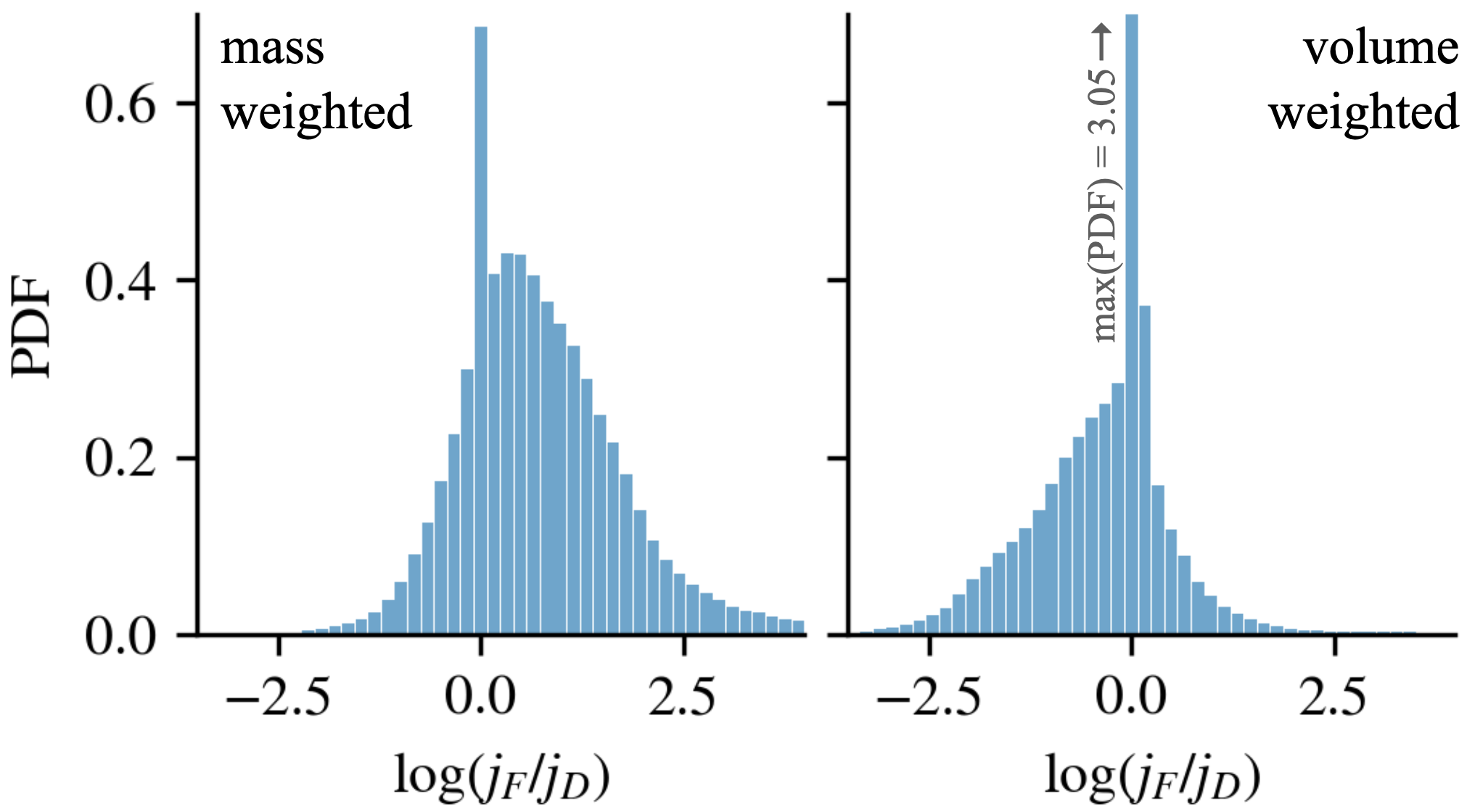
Figure 2: The 1D PDF of $\log j_{F}/j_{D}$, weighted by mass (left) and volume (right). Each PDF is composed of a population of cells that are in CSS (the peak at $\log j_{F}/j_{D}=0$), and a wide and prominent distribution of gas that is out-of-CSS (see also Table 1).

Quantity		True	Observed	Relative difference (%)
Total H2 formation rate	$\dot{M}_{\rm F}$	$8.6\times 10^{3}$ $({\rm M_{\odot}/Myr})$	$(9.3,10.9,7.3)\times 10^{3}$ $({\rm M_{\odot}/Myr})$	$(8,26,-15)$
Total H2 dissociation rate	$\dot{M}_{\rm D}$	$1.1\times 10^{3}$ $({\rm M_{\odot}/Myr})$	$(1.4,1.5,1.1)\times 10^{3}$ $({\rm M_{\odot}/Myr})$	$(23,29,-6)$
Net H2 formation rate	$\dot{M}_{\rm H_{2}}$	$7.5\times 10^{3}$ $({\rm M_{\odot}/Myr})$	$(7.9,9.4,6.2)\times 10^{3}$ $({\rm M_{\odot}/Myr})$	$(6,26,-17)$

Table 2: Integrated H₂ formation and dissociation rate statistics (see Eqs. 14, 15). The relative difference is defined as (obs-true)/true. The observed integrated rates (integrated over the entire cloud) recover the true rates to within 29%.

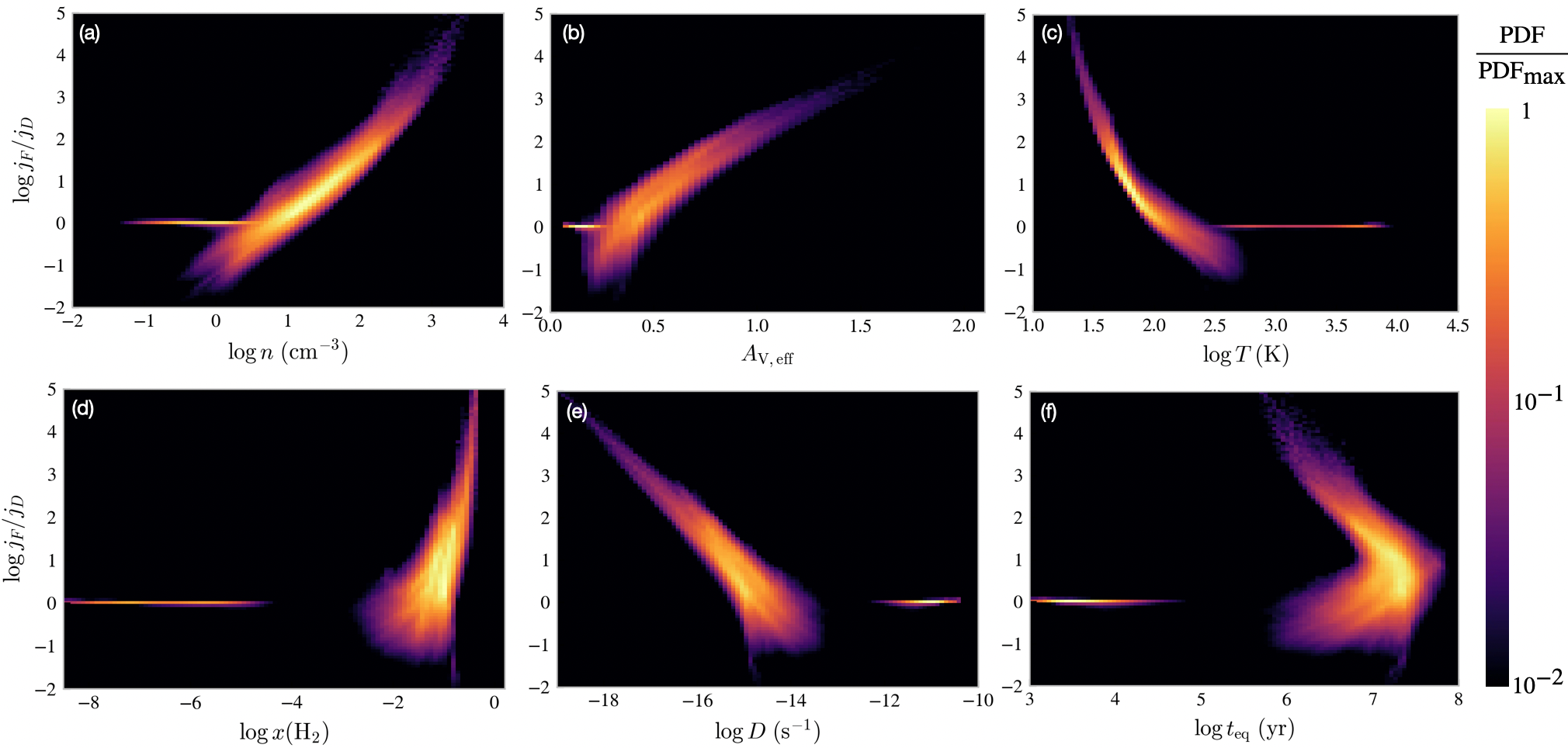
Figure 3: Mutual 2D mass-weighted PDFs of volumetric quantities in the simulation box. We show 2D PDFs of $\log j_{F}/j_{D}$ versus (a) gas density; (b) effective dust extinction; (c) gas temperature; (d) H₂ fraction; (e) local (attenuated) photodissociation rate; (f) chemical timescale (see text for details). These PDFs reveal two distinct populations: [1] A warm, diffuse and H₂-poor gas, located in low-shielded regions, that has achieved CSS (i.e., the narrow horizontal strips at $\log j_{F}/j_{D}=0$) and [2] Cold, dense, H₂-rich, well-shielded gas, that is out of CSS and exhibits a wide $j_{F}/j_{D}$ distribution.

4 Results

4.1 Volumetric quantities

Before presenting the integrated H₂ formation/dissociation rates, we begin by exploring key volumetric quantities. This provides intuition regarding the conditions in the simulation box. On all figures, $\log$ denotes the logarithm base 10.

Fig. 1 illustrates the cloud’s density structure and its chemical state. It shows a 2D slice parallel to the $xy$ plane sliced at the middle of the $z$ axis. The six panels correspond to various fields: the gas density $n$, the gas temperature $T$, the H₂ abundance $x({\rm H_{2}})\equiv n({\rm H_{2}})/n$, the local H₂ (shielded) photodissociation rate $D$ (Eq. 4), and the volumetric H₂ formation and photodissociation rates, $j_{F}$ and $j_{D}$ (Eq. 2). The gas is highly inhomogeneous, with density and temperature spanning large ranges. Due to absorption of the FUV radiation, the cloud interior is mostly cold, with $T\lesssim 100$ K. This attenuation of the radiation intensity with cloud depth is also evident in the maps of $x({\rm H_{2}})$ and $D$ where we see a sharp decrease in the photodissociation rate, and a sharp increase in the H₂ abundance from cloud edge to the cloud interior. The clumpy density structure of the cloud, as well as time-dependent chemical effects, result in inhomogenous structures of $j_{F}$ and $j_{D}$ where often the two are not in balance.

In Fig. 2 we present the probability density function (PDF) of $j_{F}/j_{D}$ (Eq. 2), weighted by mass (left) and by volume (right). The PDFs are composed of two components: a sharp peak at $\log j_{F}/j_{D}=0$ which arises from gas cells that are in CSS, and a broad component spanning a large range of out-of-CSS gas.

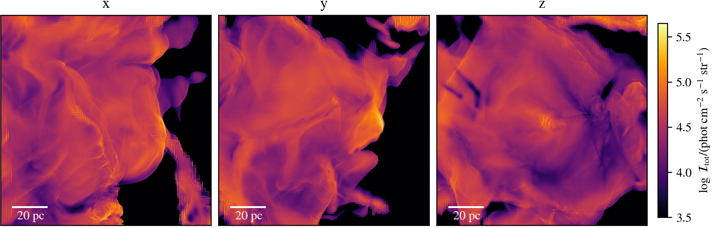
Figure 4: H₂ line emission maps. The panels show the H₂ emission line intensity (summed over all emission lines), for three orientations of the observer’s LOS (see §3.2 for details).

To get insight onto these two populations, in Fig. 3 we plot the joint distribution (mass-weighted) of $j_{F}/j_{D}$ versus various volumetric quantities: (a) the gas number density $n$; (b) the effective dust extinction $A_{\rm V,eff}$ (c) the gas temperature, $T$; (d) the H₂ abundance $x({\rm H_{2}})$; (e) the local H₂ photodissociation rate, $D$ (Eq. 4); (f) the timescale required to reach CSS, $t_{\rm chem}$ (Eq. 5). Looking at the 2D distributions in Fig. 3, we see these two populations. In the upper panels we see that the CSS population corresponds to gas that is relatively diffuse and warm, with $n\sim 0.1-3$ cm^-3 and $T\approx 300-6000$ K, and has low visual extinctions, $A_{\rm V,eff}\lesssim 0.25$. This gas is located closer to the cloud boundaries and is exposed to relatively strong FUV radiation. Indeed, from the $D$ and $x_{\rm H_{2}}$ PDFs, we see that the CSS gas experiences high dissociation rates $D\approx 10^{-12}-10^{-10}$ s^-1 (i.e., little attenuation), and is predominantly atomic with $x({\rm H_{2}})\lesssim 10^{-5}$. The timescale to achieve CSS for such conditions is the H₂ photodissociation time and is very short, $t_{\rm chem}\simeq 1/D\sim(0.03-3)\times 10^{4}$ yrs, and thus the gas is in CSS.

The gas that is in CSS occupies a significant volume fraction, however, it includes only a small fraction of the MC mass. Most of the mass is found in out-of-CSS gas (see also Seifried et al., 2022). This population shows up in Fig. 3 as the wide distribution of pixels extending from $\log j_{F}/j_{D}\sim-2$ to $\sim 4$. This gas is typically denser and colder, $n\sim 1-10^{3}$ cm^-3, $T\approx 20-300$ K, and is located in inner cloud regions with $A_{\rm V,eff}=0.25-1.5$. This gas is exposed to low FUV intensities ($D\lesssim 10^{-14}$ s^-1) and is H₂-rich ($x({\rm H_{2}})\gtrsim 10^{-2}$). Under these conditions, the chemical timescale is long, $t_{\rm chem}\simeq 1/(2Rn)\approx 1\text{--}100~{}\text{Myr}$, and the gas has not had sufficient time to reach CSS.

Qualitatively, defining CSS as regions where the H₂ formation and dissociation rates differ by less than a factor of two (i.e., $0.5<(j_{F}/j_{D})<2$), we find that only 26 % of the simulation mass is in CSS (see Table 1). The volume fraction of cells that are in CSS is 59 %. The volume fraction is higher than the mass fraction because the CSS regions reside near cloud boundaries where the gas is typically more diffuse and thus occupies larger volumes.

Integrating $j_{F}$ and $j_{D}$ over the MC volume, we obtain the total H₂ formation and dissociation rates. We find:

$$\dot{M}_{\rm F} =\bar{m}\iiint j_{F}\ \mathrm{d}V=8.6\times 10^{3}\ \mathrm{M_{\sun}\ Myr^{-1}},$$ (14)

$$\dot{M}_{\rm D} =\bar{m}\iiint j_{D}\ \mathrm{d}V=1.1\times 10^{3}\ \mathrm{M_{\sun}\ Myr^{-1}}\ ,$$

and a net H₂ mass formed per unit time $\dot{M}_{\rm H_{2}}=\dot{M}_{F}-\dot{M}_{D}=7.5\times 10^{3}\ \mathrm{M_{\sun}\ Myr^{-1}}$ (see Table 2, and see also Eq. 15). This net positive formation rate indicates that if the cloud were to maintain these gas conditions for a sufficiently long time ($t>t_{\rm chem}$), a significant mass of Hi would eventually convert to H₂. Consequently, the reduced Hi fraction would cause $j_{F}$ to decrease (see Equation 2) until it finally equilibrates with $j_{D}$, at which point the gas reaches CSS. In Paper II of this series (Burkhart et al., 2024), we explore the evolution of H₂ formation and dissociation rates over the dynamical timescales of MCs.

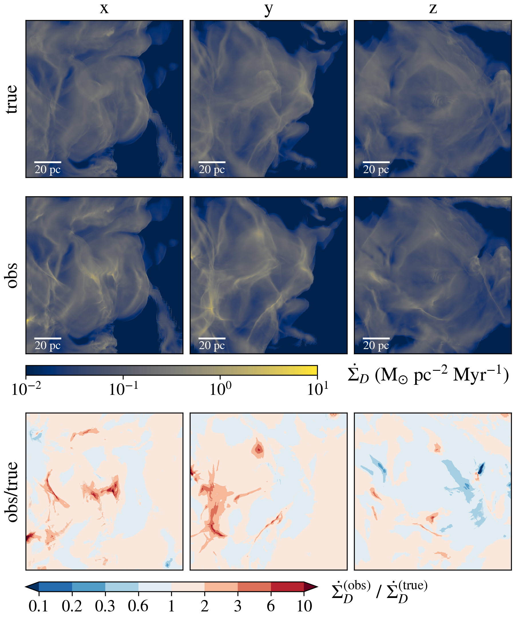
Figure 5: Integrated H₂ photodissociation rate maps. Top: maps of the true photodissociation rate, $\dot{\Sigma}_{D}^{\rm(true)}$, as calculated by integrating the volumetric photodissociation rate (Eq. 7). Middle: The observationally-derived rate, $\dot{\Sigma}_{D}^{\rm(obs)}$, as derived from the H₂ line emission map, $\mathcal{I}_{\rm tot}$ (Eq. 9; §3.2). 3^rd Bottom: The ratio $\dot{\Sigma}_{D}^{\rm(obs)}/\dot{\Sigma}_{D}^{\rm(true)}$.

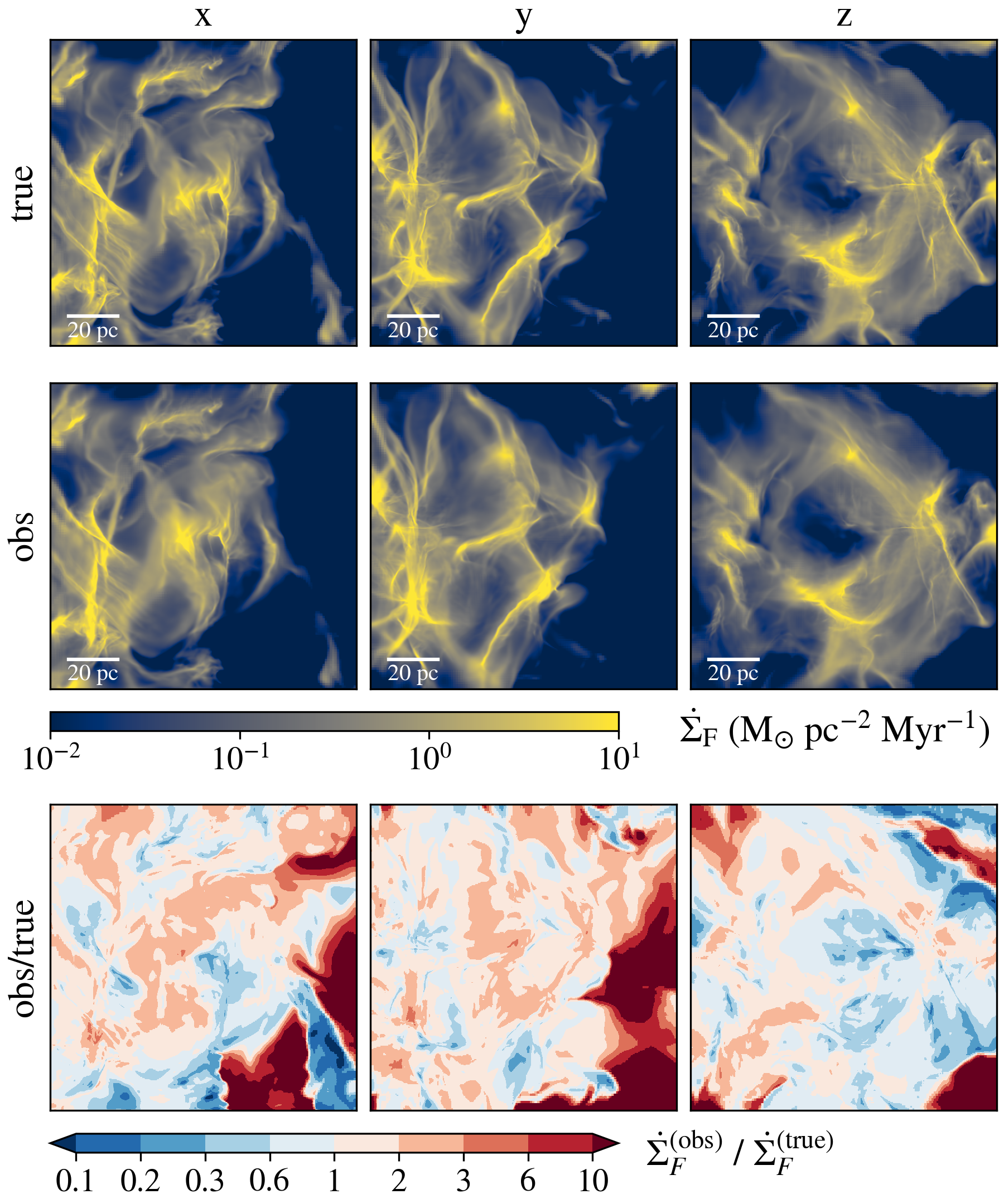
Figure 6: As Fig. 5, but for the H₂ formation rate.

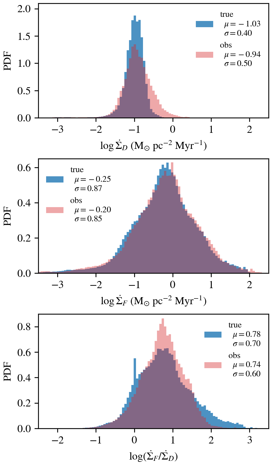
Figure 7: Mass-weighted rate PDFs. The PDF of the H₂ photodissociation rate, $\log\dot{\Sigma}_{D}$ (top), the H₂ formation rate, $\log\dot{\Sigma}_{F}$ (middle) and their ratio, $\log(\dot{\Sigma}_{F}/\dot{\Sigma}_{D})$ (bottom). For these PDFs we stacked data for the three LOS orientations, $x$, $y$, $z$. Each panel compares the observationally-derived (Eqs. 9, 12) and the true (Eq. 7) rate PDFs . The mean and standard deviations are indicated.

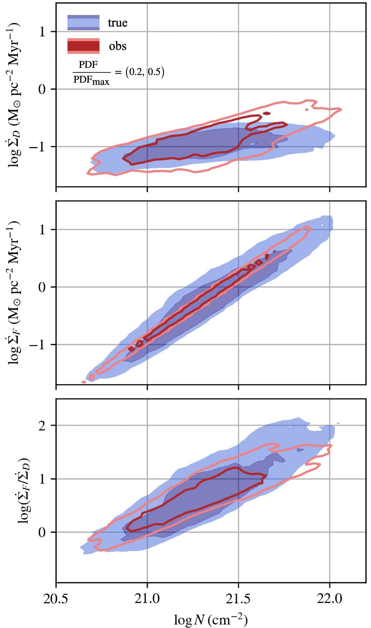
Figure 8: Mass-weighted mutual 2D PDFs of $\log N$, the total gas column density along the LOS, versus $\log\dot{\Sigma}_{D}$ (top), $\log\dot{\Sigma}_{F}$ (middle) and $\log(\dot{\Sigma}_{F}/\dot{\Sigma}_{D})$ (bottom). The red and blue PDFs correspond to the observationally-derived (Eqs. 9, 12) and the true (Eq. 7) rate PDFs respectively. The light and dark red contours correspond to PDF/PDF${}_{\rm max}=0.2$ and 0.5, respectively. Similarly, the light blue shows the level $0.2\leq{\rm PDF/PDF_{\rm max}}<0.5$ and the darker blue shows the PDF region of ${\rm PDF/PDF_{\rm max}}\geq 0.5$.

4.2 2D Maps

Fig. 4 presents maps of the total H₂ line emission, $\mathcal{I}_{\rm tot}$, for three LOS orientations, generated following the procedure described in § 3.2. These maps simulate the observations an astronomer might obtain by directing an FUV spectrograph towards an MC and aggregating all observed H₂ line intensities.

Fig. 5 compares the 2D maps of the true H₂ photodissociation rate, $\dot{\Sigma}_{D}^{\rm(true)}$, and the observer-derived rate, $\dot{\Sigma}_{D}^{\rm(obs)}$. The true rate is calculated by integrating the volumetric photodissociation rate cell-by-cell in the simulation (Eq. 7), while the observer-derived rate is obtained from the H₂ line emission maps (Eq. 9; see also §3.2). For the three LOS orientations, the observer-derived maps effectively recover the true H₂ dissociation maps over a large dynamic range of photodissociation rates, from $\dot{\Sigma}_{D}=10^{-2}$ to $10\ M_{\odot}$ pc^-2 Myr^-1. As discussed in §2.2.1, the observationally-derived rates and true rates are not identical because an observer does not have access to the true value of the attenuation factor and must rely on integrated quantities (i.e., Eq. A5 vs. Eq. A3).

Fig. 6 shows the true and observationally-derived H₂ formation rate maps. Here again, we observe that the overall structure of the observationally-derived H₂ formation rate map qualitatively agrees with the true formation rate map, spanning from weakly H₂-forming regions with $\dot{\Sigma}_{F}=0.01\ M_{\odot}$ pc^-2 Myr^-1 to highly efficient H₂-forming regions with $\dot{\Sigma}_{F}=10\ M_{\odot}$ pc^-2 Myr^-1.

When summing $\dot{\Sigma}_{D}$ and $\dot{\Sigma}_{F}$ over the entire area of the map, we obtain the total H₂ formation and dissociation rate,

$$\dot{M}_{F} \equiv\iint\dot{\Sigma}_{F}\mathrm{d}A\quad,\quad\dot{M}_{D}\equiv\iint\dot{\Sigma}_{D}\mathrm{d}A\ ,$$ (15)

and the net H₂ mass formed per unit time, $\dot{M}_{\rm H_{2}}=\dot{M}_{F}-\dot{M}_{D}$. In Table 2, we present the observationally derived values of $\dot{M}_{F}$, $\dot{M}_{D}$, and $\dot{M}_{\rm H_{2}}$ for the three LOS orientations, and compare them with the true integrated rates (which do not depend on orientation). We find that for the H₂ formation rate, the relative difference, $(\text{obs}-\text{true})/\text{true}$, ranges within 8 and 26%. For H₂ dissociation, the relative difference is within -6% and 29%, and for the net rate, the relative difference is within -17% and 26%. We provide an additional quantitative comparison of the true and observed formation and dissociation rates in the following section.

4.3 PDFs of $\dot{\Sigma}_{D}$ and $\dot{\Sigma}_{F}$

Fig. 7 shows the mass-weighted PDFs of $\dot{\Sigma}_{D}$, $\dot{\Sigma}_{F}$ and $\dot{\Sigma}_{F}/\dot{\Sigma}_{D}$. For these PDFs, we stack the data for the three LOS orientations, $x$, $y$, $z$. In each panel, the blue histograms correspond to the true rates, and the red to the observationally-derived rates. Qualitatively, the observational PDFs provide a good approximation to the true PDFs, recovering the general shape, average position and PDF dispersion. Quantitatively, we find that there are (small) statistical differences. For example, the mass-weighted average and standard deviation of $\log\dot{\Sigma}_{D}$ are $(\mu,\sigma)=(-1.03,0.40)$ for the “true” PDF, and $(-0.94,0.50)$ for the “observed” PDF. For $\log\dot{\Sigma}_{F}$ we find $(\mu,\sigma)=(-0.25,0.87)$ for the “true” PDF, and $(-0.20,0.85)$ for the “observed” PDF.

Comparing the PDFs in the top vs the middle panels, we see that the formation-rate PDFs have significantly larger dispersion compared to the dissociation-rate PDFs. This high dispersion in $\dot{\Sigma}_{F}$ is driven by the strong density fluctuations of the cloud, and the fact that for a significant fraction of the cloud mass the gas has not yet reached CSS (see §4.1).

This is further demonstrated in Fig. 8. in which we show the joint (2D) mass-weighted PDFs of $\dot{\Sigma}_{F}$, $\dot{\Sigma}_{D}$, and $\dot{\Sigma}_{F}/\dot{\Sigma}_{D}$, versus the gas column density $N$. Both formation and dissociation rates systematically increase with $N$. However, the formation rate has a steeper slope. Consequently, at large column densities, the H₂ formation rate surpasses the photodissociation rate. As discussed in § 4.1, the cloud regions contributing to this excess formation are areas with high volume density, typically embedded deep in the cloud, which are in the process of converting Hi into H₂ and have not yet reached CSS. If the MC were to maintain its physical conditions for a sufficiently long time ($\gg t_{\rm chem}$), these regions would eventually convert most of their Hi into H₂, reducing the formation rate until it balances with the dissociation rate. Such balance has already been achieved (approximately) in the more diffuse cloud regions, at $N\lesssim 10^{21}~{}\mathrm{cm}^{-2}$.

Fig. 8 also highlights cloud regions where our method performs well statistically and where it is less accurate. For H₂ dissociation, in less dense cloud regions ($N\lesssim 2\times 10^{21}~{}\mathrm{cm}^{-2}$), the observationally derived rates closely match the true rates. In denser regions, however, the observationally derived rates generally overestimate the true rate. At $N=3\times 10^{21}~{}\mathrm{cm}^{-2}$, this overestimation is typically a factor of 1.4 (comparing the means of the two PDFs), whereas at $N=10^{22}~{}\mathrm{cm}^{-2}$, the observational PDF’s performance further declines, with the overestimation increasing to a factor of 2.2. As we discuss in § 5.2, our method is not reliable at large columns in any case, as CR dissociation may become significant in such environments. For H₂ formation, the observationally derived PDF statistically recovers the true PDF over the entire range of $N$. However, at any given $N$, it exhibits a systematically lower dispersion compared to the true rate PDF.

These results demonstrate both the potential and limitations of our observational method for deriving H₂ formation and dissociation rates across various cloud conditions, setting the stage for a more detailed examination of its implications and applicability, which we discuss in the following section.

5 Discussion

As we showed in this paper, large fractions of clouds’ masses may be far from CSS, with H₂ formation and dissociation not balancing each other. We demonstrated that observations of H₂ emission lines, in combination with gas column densities, may be used to constrain the H₂ formation and dissociation rates and to assess whether the gas along the observation LOS is in CSS.

5.1 Generalization to IR line emission

Since FUV line emission from H₂ excitation is followed by rovibrational cascades within the ground electronic state, it is accompanied by IR line emission (van Dishoeck & Black, 1986; Black & van Dishoeck, 1987; Sternberg, 1988; Sternberg & Dalgarno, 1989). This H₂ line emission has been observed in a variety of sources (e.g., Gatley et al., 1987; Puxley et al., 1988; Dinerstein et al., 1988; Tanaka et al., 1989; Tanaka et al., 1991; Kaplan et al., 2021). These IR emission lines can also be used to estimate the integrated H₂ photodissociation rate.

While IR line emission can be used to derive the H₂ photodissociation rate, a complication arises because these transitions originate from ro-vibrationally excited H₂ states, which can be excited by various mechanisms beyond photo-excitation, including collisional excitation in warm gas regions (e.g., shocks), secondary electrons produced by penetrating cosmic rays or X-rays, and chemical pumping during H₂ formation (Fig. 1 in Bialy 2020). Consequently, deducing the H₂ photodissociation rate ($\dot{\Sigma}_{D}$) requires disentangling these various excitation processes. In contrast, FUV lines solely originate from photo-excitation, providing a more direct relation to the H₂ photodissociation rate, although IR line emission has the advantage of being less affected by dust extinction, allowing probing of deeper cloud regions. Ideally, both FUV and IR lines should be used in tandem to (a) verify the consistency of the H₂ dissociation rate derived from both methods, (b) assess the impact of dust extinction on H₂ line emission, and (c) determine the roles of the various excitation mechanisms.

Assuming the subtraction of H₂ line emission due to the alternative excitation processes, we may write a relation for the H₂ photodissociation rate in terms of the IR line emission. Following the derivation of Eq. (A4) (see Appendix) we obtain:

$$\dot{\Sigma}_{D}^{\rm(obs)} =\frac{4\pi p_{\rm diss}\bar{m}}{(1-p_{\rm diss})\ \mathcal{N}^{\rm IR}}\ \mathcal{I}_{\rm tot}^{\rm IR}$$ (16)

$$=4.4\times 10^{-2}\ \mathcal{I}_{5}^{\rm IR}\ {\rm M_{\odot}\ pc^{-2}\ Myr^{-1}}\ ,$$

where $\mathcal{I}_{\rm tot}^{\rm IR}$ is the IR total line intensity, and $\mathcal{I}_{5}\equiv\mathcal{I}_{\rm tot}^{\rm IR}/(10^{5}$ photons cm^-2 s^-1 str^-1). In Eq. (16) we do not include the dust attenuation $\beta_{\rm dust}$ factor (Eq. A3, A5) because for the IR wavelength dust absorption is typically negligible. For a dust absorption cross section of $4.5\times 10^{-23}$ cm² per hydrogen nucleus (for the 2–3 $\mu$m wavelength range; Draine 2011), the gas remains optically thin up to gas column densities $N\approx 2\times 10^{22}$ cm^-2.

The factor $\mathcal{N}^{\rm IR}=\mathcal{I}_{\rm tot}^{\rm IR}/\mathcal{I}_{\rm tot}$ is the ratio of IR to FUV photons emitted per H₂ photo-excitation. This factor arises because IR emission involves cascades through multiple rovibrational states, unlike FUV emission where each excitation produces a single photon. For instance, when the excited H₂ state $B^{1}\Sigma^{+}_{u}$ decays to $X^{1}\Sigma^{+}_{g}$, it emits one FUV photon and leaves H₂ rovibrationally excited, which may then emit multiple IR photons (e.g., three photons in the path $v=3\rightarrow 2\rightarrow 1\rightarrow 0$). Using the Meudon PDR code data (Le Petit et al., 2006), we calculated $\mathcal{N}^{\rm IR}$ for various gas temperatures, considering photo-pumping from $X^{1}\Sigma^{+}_{g}$ to excited levels within $B^{1}\Sigma^{+}_{u}$ and $C^{1}\Pi^{u}$, assuming a Boltzmann distribution for $X^{1}\Sigma^{+}_{g}$ rovibrational states and a Draine (1978) FUV radiation spectrum. Using Einstein $A$ coefficients, we computed decay probabilities and the resulting FUV and IR line emissions. For $T=100$ K, we found $\mathcal{N}^{\rm IR}=3.6$, a value that varies little (standard deviation 0.09, min-max variation 0.3) for temperatures between 10 and 1000 K, indicating that $\mathcal{N}^{\rm IR}$ remains relatively constant across a wide range of temperatures relevant to molecular clouds.

While in terms of photon number, the total IR line emission is higher, the energy surface brightness (erg cm^-2 s^-1 sr^-1) is greater in the FUV, due to the higher energies carried by the FUV photons.

5.2 Additional H₂ destruction processes

Our model focuses on H₂ photodissociation, neglecting other destruction mechanisms such as cosmic ray (CR) ionization and dissociation, X-ray ionization, and collisional dissociation in warm/hot gas. It is thus best suited for standard molecular clouds that are typically cold ($\ll 10^{4}$ K) and not exposed to abnormally strong X-ray or CR fluxes. In the Appendix, we describe a detailed model explicitly calculating the effect of CR ionization on H₂ removal rate compared to FUV photodissociation. For a typical CR ionization rate of $\zeta_{0}=10^{-16}$ s^-1, CR destruction remains negligible compared to photodissociation for lines of sight with column densities $N\lesssim 2\times 10^{22}$ cm^-2 (see Appendix and Fig. 9), consistent with analytic model predictions (Sternberg et al., 2024). X-rays similarly affect H₂ destruction, producing secondary electrons that lead to H₂ ionization and dissociation analogous to CRs.

In regions with abnormally high CR or X-ray fluxes, an apparent imbalance between H₂ formation and dissociation rates (as measured by FUV emission lines) may be observed, even if H₂ is in CSS, because FUV emission lines only reflect the contribution from FUV excitation and photo-dissociation, not the total H₂ removal rate (although at sufficiently high fluxes or column densities, CRs may also contribute to FUV line emission; Padovani et al. 2024). For such clouds, the additional contribution of CR ionization and dissociation to H₂ removal can be constrained by observing various molecular ions (e.g., H${}_{3}^{+}$, OH⁺, H₂O⁺, ArH⁺) in absorption spectroscopy (e.g., van der Tak & van Dishoeck, 2000; Indriolo & McCall, 2012; Neufeld & Wolfire, 2017; Bialy et al., 2019). Alternatively, the CR contribution may be derived from H₂ observations by targeting specific IR emission lines (within the 2-3 $\mu$m range) produced by CR-excited H₂, with the relative contribution of CR-excited versus UV-excited H₂ lines constrained by line ratios (Bialy, 2020; Padovani et al., 2022; Gaches et al., 2022). These lines may be observable with the NIRSpec spectrograph on JWST or, for exceptionally bright CR fluxes, by ground-based observatories (Bialy et al., 2022, 2024).

5.3 Observations of H₂ in the FUV and IR

The H₂ IR emission lines can be observed with JWST’s complementary instruments: NIRSpec and MIRI. NIRSpec (Jakobsen et al., 2022) offers low resolution ($R=100$) prism spectroscopy over the entire wavelength range $\lambda=0.6-5.3$ $\mu$m, as well as medium-to-high resolution ($R=1000-2700$) gratings covering various wavelength intervals within this range. The MIRI instrument (Bouchet et al., 2015) extends the observable H₂ IR line emission spectrum to longer wavelengths.

No FUV instrument has had or currently has the ability to resolve the H₂ fluorescent lines over the large solid angles spanned by MCs. FUV H₂ emission from individual protoplanetary disks was measured by HST COS (Herczeg et al., 2004, 2006) and rocket-borne experiments (Hoadley et al., 2014, 2016). Measurements spanning 70% of the sky with the FIMS/SPEAR mission (Jo et al., 2017) showed intense H₂ emission from star-forming regions across our Galaxy. However, the spectral resolution of less than 1,000 was too low to separate the fluorescent lines and determine the excitation conditions, while the spatial resolution of about $5^{\prime}$ was coarser than the clouds’ scales of variation, leading to great uncertainty in characterizing the H₂ formation and dissociation rates in even the nearest clouds.

Building on an initial proposal for a Medium Explorer-class space telescope (Hamden et al., 2022), we have refined the concept to match NASA’s Small Explorer opportunity. This revised mission, named Eos, is designed to measure FUV lines from nearby star-forming regions with spectral resolution $R>10,000$, sufficient to distinguish individual fluorescent lines. Eos would achieve angular resolution of a few arcseconds over a spectrograph slit several degrees long, enabling detailed resolution of cloud structures while providing coverage adequate to assess global evolutionary states. This telescope would implement the measurement approach outlined in this paper, determining the extent of MCs out of CSS and addressing fundamental questions about cloud origins, evolution, and dispersal in their role as stellar nurseries.

6 Conclusions

In this study, we have investigated the photodissociation and formation processes of H₂ in simulated molecular clouds (MCs), with a particular focus on utilizing FUV and IR line emissions to constrain these rates. Our key findings are as follows:

1. A significant fraction of MC mass and volume is out of chemical steady state (CSS) due to rapid dynamical evolution, with H₂ formation rates either exceeding or lagging behind photodissociation rates (Tables 1-2).

2. The total intensity of H₂ line emission, whether measured in FUV or IR, can effectively constrain the line-of-sight (LOS) integrated H₂ photodissociation rate $\dot{\Sigma}_{D}$ (Eqs. 9, 16).

3. Measurements of HI and total gas column density provide a means to constrain the integrated H₂ formation rate, $\dot{\Sigma}_{F}$ (Eq. 12).

4. By combining H₂ line emission and gas column densities, we can determine the chemical state of gas along the LOS: CSS ($\dot{\Sigma}_{F}/\dot{\Sigma}_{D}\approx 1$), active H₂ formation ($\dot{\Sigma}_{F}/\dot{\Sigma}_{D}\gg 1$), or active photodissociation ($\dot{\Sigma}_{F}/\dot{\Sigma}_{D}\ll 1$) (Eq. 13).

5. CSS assessment reveals key aspects of MC evolution. MCs far from CSS suggest recent rapid changes - either fresh gas inflow or quick evaporation. These changes happen faster than the time needed for chemical balance (Eq. 5).

These findings provide valuable insights into the dynamics of H₂ in MCs and offer observational strategies to probe the chemical and physical states of these complex systems. Our results underscore the importance of considering non-steady-state conditions in MC studies and highlight the potential of using molecular line emissions as diagnostic tools for cloud evolution.

SB acknowledges financial support from the physics department at the Technion, and from the Center for Theory and Computational (CTC) at the University of Maryland College Park. DS and SW thank the Deutsche Forschungsgemeinschaft (DFG) for funding through the SFB 956 “The conditions and impact of star formation” (sub-projects C5 and C6). Furthermore, DS and SW receive funding from the programme “Profilbildung 2020”, an initiative of the Ministry of Culture and Science of the State of North Rhine-Westphalia. TJH is funded by a Royal Society Dorothy Hodgkin Fellowship and UKRI ERC guarantee funding (EP/Y024710/1). B.B. acknowledges support from NSF grant AST-2009679 and NASA grant No. 80NSSC20K0500. B.B. is grateful for generous support by the David and Lucile Packard Foundation and Alfred P. Sloan Foundation. The work was carried out in part at the Jet Propulsion Laboratory, California Institute of Technology, under a contract with the National Aeronautics and Space Administration. The calculations were carried out using the Numpy and Scipy libraries (Harris et al., 2020; Virtanen et al., 2020) The figures were produced using the matplotlib library (Hunter, 2007). The interactive figure was produced using Plotly and Github.

Appendix A The $\dot{\Sigma}_{D}-\mathcal{I}_{\rm tot}$ relation

We derive the relationship between the integrated H₂ photodissociation rate, $\dot{\Sigma}_{D}$, and the total H₂ line emission intensity, $\mathcal{I}_{\rm tot}$. Following S89, the total photon intensity for a uniform density 1D slab is given by

$$\mathcal{I}_{\rm tot} =\frac{1}{4\pi}(1-p_{\rm diss})\int_{0}^{L}n({\rm H_{2}})\chi P_{0}\mathrm{e}^{-2\tau}f_{\rm H_{2},shield}\mathrm{d}s$$ (A1)

$$=\frac{1}{4\pi}(1-p_{\rm diss})\int_{0}^{L}n({\rm H_{2}})P\mathrm{e}^{-\tau}\mathrm{d}s\ .$$ (A2)

To derive this relation, we start with Eq. (A1) in S89, which describes the intensity of a single H₂ emission line. We sum over the branching ratios (denoted as $b$ in S89) for transitions to bound rovibrational states, introducing the factor $(1-p_{\rm diss})$ in our Eqs. (A1-A2). In these equations, $P_{0}$ is the un-attenuated photo-excitation rate for a unit Draine (Draine, 1978) radiation field, while $P$ is the local, attenuated H₂ photo-excitation rate at cloud depth $s$. For slab geometry, $P=\chi P_{0}f_{\rm H_{2},shield}\mathrm{e}^{-\tau}$, where $f_{\rm H_{2},shield}$ is the H₂ self-shielding function (e.g., Draine & Bertoldi, 1996), and $\tau=\int_{0}^{s}\sigma n\mathrm{d}s^{\prime}$ is the dust opacity from point $s$ to the cloud’s edge, with $\sigma=1.9\times 10^{-21}$ cm² being the dust absorption cross-section per hydrogen nucleus averaged over the LW band.

Our notation differs from S89: our $P_{0}$ and $D_{0}$ correspond to their $P$ and $D$, and they denote H₂ self-shielding as $f(N_{2})$. In Eqs. (A1-A2), we integrate emission through the cloud (from $s=0$ to $s=L$) along the LOS. The factor of two in the exponent of Eq. (A1) accounts for dust absorption in both directions: first, as LW radiation propagates from the cloud edge inward, exciting H₂, and second, as the resulting emission lines travel outward. Unlike FUV continuum radiation, which experiences both dust absorption and H₂ self-shielding, H₂ emission lines are primarily attenuated by dust alone. This is because most H₂ in the cloud occupies low ro-vibrational states and thus doesn’t re-absorb these emission lines which mostly correspond to high rovibrational lower states. However, this approach is an approximation, as some self-absorption can occur, and may alter the H₂ emission spectrum at shorter wavelengths (Le Bourlot, private communication).

Examining Eq. (A2), we notice its similarity to $\dot{\Sigma}_{D}^{\rm(true)}$ (Eq. 7), differing only by a constant multiplication term and an exponential term in the integral. To express $\mathcal{I}_{\rm tot}$ in terms of $\dot{\Sigma}_{D}^{\rm(true)}$, we first define an effective attenuation factor:

$$\beta_{\rm dust}\equiv\frac{\int n({\rm H_{2}})D\mathrm{e}^{-\tau}\mathrm{d}s}{\int n({\rm H_{2}})D\mathrm{d}s}\ .$$ (A3)

Using this definition, we can combine Eq. (A2) with Eq. (7) to derive a relation between the H₂ line intensity and the integrated H₂ photodissociation rate:

$$\mathcal{I}_{\rm tot}=\frac{1-p_{\rm diss}}{4\pi p_{\rm diss}\bar{m}}\beta_{\rm dust}\ \dot{\Sigma}_{D}^{\rm(true)}\ .$$ (A4)

In this derivation, we utilize the relationship $P=D/p_{\rm diss}$ (Eq. 8).

The $\beta_{\rm dust}$ factor accounts for the reduction in line emission due to dust absorption as photons propagate from the cloud interior to the observer. However, direct measurement of $\beta_{\rm dust}$ is challenging as it depends on the 3D density structure along the LOS and the radiation geometry. While 3D dust maps provide information on density structure (e.g., Leike et al. 2020), they typically cannot resolve the critical HI-to-H₂ transition length, which usually occurs over scales $\lesssim 1$ pc (Bialy et al., 2017). In the absence of 3D information, we approximate $\beta_{\rm dust}$ using the simplest possible geometry: a 1D uniform slab where H₂ line emission and dust absorption occur, with total dust optical depth $\tau_{\rm tot}=\int_{0}^{L}\sigma nds=\sigma N$, where $N$ is the integrated gas column density along the entire LOS. Assuming equal line emission per unit dust optical depth $d\tau$, we can express $\beta_{\rm dust}$ as:

$$\beta_{\rm dust}^{\rm(obs)}=\int_{0}^{\tau_{\rm tot}}\left(\frac{\mathrm{d}\tau}{\tau_{\rm tot}}\right)\mathrm{e}^{-\tau}=\frac{1-\mathrm{e}^{-\tau_{\rm tot}}}{\tau_{\rm tot}}=\frac{1-\mathrm{e}^{-1.9N_{21}}}{1.9N_{21}}\ .$$ (A5)

This expression is the exact solution given by the equation of transfer for attenuation in a medium where emitters are fully mixed with absorbers, and is analogous to the escape probability formalism. In the last equality, we use $\sigma=1.9\times 10^{-21}$ cm^-2 and define $N_{21}\equiv N/(10^{21}\ {\rm cm^{-2}})$, yielding $\tau_{\rm tot}=1.9N_{21}$. In the limit $\tau_{\rm tot}\ll 1$, $\beta_{\rm dust,obs}\rightarrow 1$, approaching the optically thin limit. Conversely, when $\tau_{\rm tot}\gg 1$, $\beta_{\rm dust,obs}\rightarrow 1/\tau_{\rm tot}$. This is because in the optically thick limit, the LOS contains $\sim\tau_{\rm tot}$ transition layers (each with opacity $\sim 1$), but we receive signals only from emission lines to a depth of $\tau_{\rm tot}\sim 1$, resulting in relative emission $\propto 1/\tau_{\rm tot}$.

Substituting Eq. (A5) for $\beta_{\rm dust}$ in Eq. (A4), we obtain:

$$\dot{\Sigma}_{D}^{\rm(obs)} =\frac{4\pi p_{\rm diss}\bar{m}}{1-p_{\rm diss}}\ \mathcal{I}_{\rm tot}\ \left(\frac{\tau_{\rm tot}}{1-\mathrm{e}^{-\tau_{\rm tot}}}\right)$$ (A6)

$$=0.3\ \mathcal{I}_{5}\left(\frac{N_{21}}{1-\mathrm{e}^{-1.9N_{21}}}\right)\ {\rm M_{\odot}\ pc^{-2}\ Myr^{-1}}\ ,$$

where in the numerical evaluation we use $\tau_{\rm tot}=1.9N_{21}$ and define $\mathcal{I}_{5}\equiv\mathcal{I}_{\rm tot}/({10^{5}\ {\rm photons\ cm^{-2}\ s^{-1}\ sr^{-1}}})$. The superscript “(obs)” in Eqs. (A5) and (A6) emphasizes that these expressions provide approximations to the true attenuation factor and H₂ photodissociation rates, as they rely on observable (integrated) quantities.

Appendix B H₂ destruction by cosmic rays

To assess the contribution of cosmic rays (CRs) to H₂ removal, we calculated the individual contributions of FUV and CRs to H₂ dissociation on a cell-by-cell basis in our simulation. In each cell, the H₂ removal rate (s^-1) by CRs is:

$$D_{\rm CR}=\varphi\zeta$$ (B1)

where $\zeta$ (s^-1) is the total H₂ ionization rate by primary CRs and secondary electrons, and $\varphi$ is the number of H₂ molecules destroyed per ionization event. This includes H₂ ionization by CRs, H₂ dissociation via chemical reactions with CR-produced ions, and direct H₂ dissociation by CRs. Following Sternberg et al. (2024), we adopt $\varphi=2$. The CR ionization rate is given by:

$$\zeta=\begin{cases}\zeta_{0}&\text{if }N_{\rm eff}<N_{0}\\ \zeta_{0}\left(\frac{N_{\rm eff}}{N_{0}}\right)^{-\gamma}&\text{if }N_{\rm eff}\geq N_{0}\end{cases}$$ (B2)

This form accounts for CR attenuation as they propagate through the cloud, where $N_{\rm eff}$ represents an effective mean column density for CRs propagating in different directions, and $\zeta_{0}$, $N_{0}$ and $\gamma$ are constants. We approximate $N_{\rm eff}$ using the effective visual extinction $A_{V,{\rm eff}}$ as calculated by the SILCC simulation, with $N_{\rm eff}=1.8\times 10^{21}A_{V,{\rm eff}}$ cm^-2 (see Gaches et al., 2022, for a discussion of this approach). We consider the two CR energy spectral shape models $\mathcal{H}$ and $\mathcal{L}$ discussed by Padovani et al. (2018), for which $\gamma=0.39$ and 0.28, respectively and adopt the standard values $N_{0}=10^{19}$ cm^-2 and $\zeta_{0}=10^{-16}$ s^-1 (Sternberg et al., 2024). Using these equations, we calculate the H₂ removal rate by CRs on a cell-by-cell basis. We then integrate these rates along the LOS (Eq. 7) to obtain the CR contribution to the H₂ integrated removal rate, $\dot{\Sigma}_{D}$.

In Fig. 9, we present the FUV and CR contributions to $\dot{\Sigma}_{D}$ as a function of the column density along the LOS, $N$. The left and right panels correspond to the $\mathcal{L}$ and $\mathcal{H}$ CR spectral shape models, respectively. The three shaded regions in each panel represent contours of the 2D PDF of $\log\dot{\Sigma}_{D}$ versus $\log N$. These contours correspond to PDF/PDF_max levels in the ranges (0.03, 0.1), (0.1, 0.3), and (0.3, 1), depicted by light to dark shades, respectively. Our analysis shows that for LOS with column densities $N\lesssim 2\times 10^{22}$ cm^-2, the CR contribution to H₂ removal is negligible compared to FUV photodissociation. This finding is consistent with the analytic model predictions of Sternberg et al. (2024). It is important to note that our chosen value of $\zeta_{0}=10^{-16}$ s^-1 represents a standard CR ionization rate in the ambient ISM. However, in the vicinity of CR sources, such as supernova remnants, the CR flux may be significantly higher, resulting in an increased value of $\zeta_{0}$. In such cases, the CR distribution shown in our figure would be shifted upward in proportion to the increase in $\zeta_{0}$. Consequently, the transition point where CR-induced H₂ removal becomes comparable to FUV photodissociation would occur at lower column densities.

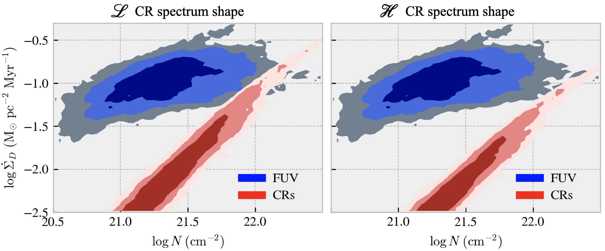
Figure 9: Contributions of FUV radiation and CRs to H₂ removal as a function of LOS column density. The left panel shows results for the $\mathcal{L}$ CR spectral shape model, while the right panel represents the $\mathcal{H}$ model (these models are discussed in Padovani et al., 2018). Both assume an unattenuated CR ionization rate of $\zeta_{0}=10^{-16}$ s^-1 and $N_{0}=10^{19}$ cm^-2 (see Eq. B1-B2). Shaded regions represent contours of the 2D PDF of $\log\dot{\Sigma}_{D}$ versus $\log N$, with light to dark shades corresponding to PDF/PDF_max levels that fall within the ranges (0.03, 0.1), (0.1, 0.3), and (0.3, 1), respectively. The figure demonstrates that for column densities $N\lesssim 2\times 10^{22}$ cm^-2, FUV photodissociation dominates over CR-induced H₂ removal, consistent with Sternberg et al. (2024).

References

- Abgrall et al. (1992) Abgrall H., Le Bourlot J., Pineau Des Forets G., Roueff E., Flower D. R., Heck L., 1992, A&A, 253, 525
- Barkana & Loeb (2001) Barkana R., Loeb A., 2001, Physics Reports, 349, 125
- Bialy (2020) Bialy S., 2020, Nature Communications Physics, 3, 32
- Bialy & Sternberg (2015) Bialy S., Sternberg A., 2015, Monthly Notices of the Royal Astronomical Society, 450, 4424
- Bialy & Sternberg (2016) Bialy S., Sternberg A., 2016, The Astrophysical Journal, 822, 83
- Bialy & Sternberg (2019) Bialy S., Sternberg A., 2019, The Astrophysical Journal, 881, 160
- Bialy et al. (2015) Bialy S., Sternberg A., Lee M.-Y., Petit F. L., Roueff E., 2015, The Astrophysical Journal, 809, 122
- Bialy et al. (2017) Bialy S., Burkhart B., Sternberg A., 2017, The Astrophysical Journal, 843, 92
- Bialy et al. (2019) Bialy S., Neufeld D., Wolfire M., Sternberg A., Burkhart B., 2019, The Astrophysical Journal, 885, 109
- Bialy et al. (2021) Bialy S., et al., 2021, The Astrophysical Journal Letters, 919, L5
- Bialy et al. (2022) Bialy S., Belli S., Padovani M., 2022, Astronomy & Astrophysics, 658, L13
- Bialy et al. (2024) Bialy S., et al., 2024, Constraining Cosmic Rays with H2 Ro-Vibrational Excitation in Dense Clouds, JWST Proposal. Cycle 3, ID. #5064
- Bigiel et al. (2008) Bigiel F., Leroy A., Walter F., Brinks E., de Blok W. J. G., Madore B., Thornley M. D., 2008, The Astronomical Journal, 136, 2846
- Bisbas et al. (2019) Bisbas T. G., Schruba A., Van Dishoeck E. F., 2019, Monthly Notices of the Royal Astronomical Society, 485, 3112
- Bisbas et al. (2021) Bisbas T. G., Tan J. C., Tanaka K. E. I., 2021, Monthly Notices of the Royal Astronomical Society, 502, 2701
- Black & van Dishoeck (1987) Black J. H., van Dishoeck E. F., 1987, The Astrophysical Journal, 322, 412
- Bouchet et al. (2015) Bouchet P., et al., 2015, PASP, 127, 612
- Bromm et al. (2001) Bromm V., Ferrara A., Coppi P., Larson R., 2001, Monthly Notices of the Royal Astronomical Society, 328, 969
- Burkhart et al. (2024) Burkhart B., et al., 2024, arXiv e-prints, p. arXiv:2402.01587
- Chevance et al. (2023) Chevance M., Krumholz M. R., McLeod A. F., Ostriker E. C., Rosolowsky E. W., Sternberg A., 2023, in Inutsuka S., Aikawa Y., Muto T., Tomida K., Tamura M., eds, Astronomical Society of the Pacific Conference Series Vol. 534, Protostars and Planets VII. p. 1 (arXiv:2203.09570), doi:10.48550/arXiv.2203.09570
- Dalgarno (2006) Dalgarno A., 2006, Proceedings of the National Academy of Sciences of the United States of America, 103, 12269
- Dalgarno et al. (1970) Dalgarno A., Herzberg G., Stephens T. L., 1970, ApJ, 162, L49
- Dawson (2013) Dawson J. R., 2013, Publications of the Astronomical Society of Australia, 30, e025
- Dinerstein et al. (1988) Dinerstein H. L., Lester D. F., Carr J. S., Harvey P. M., 1988, ApJ, 327, L27
- Draine (1978) Draine B. T., 1978, The Astrophysical Journal Supplement Series, 36, 595
- Draine (2011) Draine B. T., 2011, Physics of the Interstellar and Intergalactic Medium, doi:10.2307/j.ctvcm4hzr.
- Draine & Bertoldi (1996) Draine B. T., Bertoldi F., 1996, The Astrophysical Journal, 468, 269
- Faucher-Giguère et al. (2013) Faucher-Giguère C. A., Quataert E., Hopkins P. F., 2013, Monthly Notices of the Royal Astronomical Society, 433, 1970
- Field et al. (1966) Field G. B., Somerville W. B., Dressler K., 1966, Annual Review of Astronomy and Astrophysics, 4, 207
- Gaches et al. (2022) Gaches B. A. L., Bisbas T. G., Bialy S., 2022, Astronomy & Astrophysics, 658, A151
- Galli & Palla (1998) Galli D., Palla F., 1998, Astronomy and Astrophysics, 335, 403
- Gatley et al. (1987) Gatley I., et al., 1987, ApJ, 318, L73
- Girichidis et al. (2015) Girichidis P., et al., 2015, eprint arXiv:1508.06646
- Glover & Mac Low (2007) Glover S. C. O., Mac Low M.-M., 2007, The Astrophysical Journal, 659, 1317
- Haiman et al. (1996) Haiman Z., Rees M. J., Loeb A., 1996, The Astrophysical Journal, 467, 522
- Hamden et al. (2022) Hamden E. T., et al., 2022, Journal of Astronomical Telescopes, Instruments, and Systems, 8, 044008
- Harris et al. (2020) Harris C. R., et al., 2020, Nature, 585, 357
- Hartmann et al. (2002) Hartmann L., Ballesteros-Paredes J., Bergin E. A., 2002, The Astrophysical Journal, 562, 852
- Herbst & Klemperer (1973) Herbst E., Klemperer W., 1973, The Astrophysical Journal, 185, 505
- Herczeg et al. (2004) Herczeg G. J., Wood B. E., Linsky J. L., Valenti J. A., Johns-Krull C. M., 2004, ApJ, 607, 369
- Herczeg et al. (2006) Herczeg G. J., Linsky J. L., Walter F. M., Gahm G. F., Johns-Krull C. M., 2006, ApJS, 165, 256
- Hoadley et al. (2014) Hoadley K., et al., 2014, in Takahashi T., den Herder J.-W. A., Bautz M., eds, Society of Photo-Optical Instrumentation Engineers (SPIE) Conference Series Vol. 9144, Space Telescopes and Instrumentation 2014: Ultraviolet to Gamma Ray. p. 914406, doi:10.1117/12.2055661
- Hoadley et al. (2016) Hoadley K., et al., 2016, in den Herder J.-W. A., Takahashi T., Bautz M., eds, Society of Photo-Optical Instrumentation Engineers (SPIE) Conference Series Vol. 9905, Space Telescopes and Instrumentation 2016: Ultraviolet to Gamma Ray. p. 99052V (arXiv:1606.04979), doi:10.1117/12.2232242
- Hollenbach & McKee (1979) Hollenbach D., McKee C. F., 1979, The Astrophysical Journal Supplement Series, 41, 555
- Hollenbach & Tielens (1999) Hollenbach D. J., Tielens A. G. G. M., 1999, Reviews of Modern Physics, 71, 173
- Hopkins et al. (2020) Hopkins P. F., et al., 2020, Monthly Notices of the Royal Astronomical Society, 3498, 3465
- Hu et al. (2016) Hu C.-Y., Naab T., Walch S., Glover S. C. O., Clark P. C., 2016, Monthly Notices of the Royal Astronomical Society, 458, 3528
- Hu et al. (2021) Hu C.-Y., Sternberg A., van Dishoeck E. F., 2021, The Astrophysical Journal, 920, 44
- Hunter (2007) Hunter J. D., 2007, Computing in Science & Engineering, 9, 90
- Indriolo & McCall (2012) Indriolo N., McCall B. J., 2012, The Astrophysical Journal, 745, 91
- Jakobsen et al. (2022) Jakobsen P., et al., 2022, Astronomy & Astrophysics, 661, A80
- Jeffreson et al. (2024) Jeffreson S. M. R., Semenov V. A., Krumholz M. R., 2024, MNRAS, 527, 7093
- Jo et al. (2017) Jo Y.-S., Seon K.-I., Min K.-W., Edelstein J., Han W., 2017, The Astrophysical Journal Supplement Series, 231, 21
- Kaplan et al. (2021) Kaplan K. F., Dinerstein H. L., Kim H., Jaffe D. T., 2021, ApJ, 919, 27
- Koyama & Inutsuka (2000) Koyama H., Inutsuka S.-I., 2000, The Astrophysical Journal, 1, 980
- Krumholz (2012) Krumholz M. R., 2012, The Astrophysical Journal, 759, 9
- Krumholz et al. (2008) Krumholz M. R., McKee C. F., Tumlinson J., 2008, The Astrophysical Journal, 689, 865
- Krumholz et al. (2009) Krumholz M. R., McKee C. F., Tumlinson J., 2009, The Astrophysical Journal, 693, 216
- Le Petit et al. (2006) Le Petit F., Nehme C., Le Bourlot J., Roueff E., 2006, The Astrophysical Journal Supplement Series, 164, 506
- Leike et al. (2020) Leike R., Glatzle M., Enßlin T. A., 2020, Astronomy & Astrophysics, 138, 1
- Leroy et al. (2008) Leroy A. K., Walter F., Brinks E., Bigiel F., de Blok W. J. G., Madore B., Thornley M. D., 2008, The Astronomical Journal, 136, 2782
- Luhman et al. (1994) Luhman M. L., Jaffe D. T., Keller L. D., Pak S., 1994, The Astrophysical Journal, 436, L185
- Maloney et al. (1996) Maloney P. R., Hollenbach D. J., Tielens A. G. G. M., 1996, The Astrophysical Journal, 466, 561
- McKee & Ostriker (1977) McKee C. F., Ostriker J. P., 1977, The Astrophysical Journal, 218, 148
- McKee & Ostriker (2007) McKee C. F., Ostriker E. C., 2007, Annual Review of Astronomy and Astrophysics, 45, 565
- Neufeld & Spaans (1996) Neufeld D. A., Spaans M., 1996, The Astrophysical Journal, 473, 894
- Neufeld & Wolfire (2017) Neufeld D. A., Wolfire M. G., 2017, The Astrophysical Journal, 845, 163
- Noterdaeme et al. (2019) Noterdaeme P., Balashev S., Krogager J. K., Srianand R., Fathivavsari H., Petitjean P., Ledoux C., 2019, Astronomy and Astrophysics, 627, A32
- Ntormousi et al. (2011) Ntormousi E., Burkert A., Fierlinger K., Heitsch F., 2011, Astrophysical Journal, 731
- Omukai (2000) Omukai K., 2000, The Astrophysical Journal, 534, 809
- Orr et al. (2022) Orr M. E., Fielding D. B., Hayward C. C., Burkhart B., 2022, The Astrophysical Journal Letters, 924, L28
- Ostriker & Kim (2022) Ostriker E. C., Kim C.-G., 2022, ApJ, 936, 137
- Padovani et al. (2018) Padovani M., Galli D., Ivlev A. V., Caselli P., Ferrara A., 2018, Astronomy and Astrophysics, 619, 1
- Padovani et al. (2022) Padovani M., et al., 2022, A&A, 658, A189
- Padovani et al. (2024) Padovani M., Galli D., Scarlett L. H., Grassi T., Rehill U. S., Zammit M. C., Bray I., Fursa D. V., 2024, A&A, 682, A131
- Pound & Wolfire (2023) Pound M. W., Wolfire M. G., 2023, AJ, 165, 25
- Puxley et al. (1988) Puxley P. J., Hawarden T. G., Mountain C. M., 1988, MNRAS, 234, 29P
- Ranjan et al. (2018) Ranjan A., et al., 2018, Astronomy & Astrophysics, 618, A184
- Richings et al. (2014) Richings A. J., Schaye J., Oppenheimer B. D., 2014, Monthly Notices of the Royal Astronomical Society, 442, 2780
- Röllig & Ossenkopf-Okada (2022) Röllig M., Ossenkopf-Okada V., 2022, Astronomy and Astrophysics, 664, A67
- Röllig et al. (2007) Röllig M., et al., 2007, A&A, 467, 187
- Schruba et al. (2011) Schruba A., et al., 2011, The Astronomical Journal, 142, 37
- Schruba et al. (2018) Schruba A., Bialy S., Sternberg A., 2018, The Astrophysical Journal, 862, 110
- Seifried et al. (2017) Seifried D., et al., 2017, Monthly Notices of the Royal Astronomical Society, 472, 4797
- Seifried et al. (2019) Seifried D., Walch S., Reissl S., Ibáñez-Mejía J. C., 2019, MNRAS, 482, 2697
- Seifried et al. (2020) Seifried D., Haid S., Walch S., Borchert E. M. A., Bisbas T. G., 2020, MNRAS, 492, 1465
- Seifried et al. (2022) Seifried D., Beuther H., Walch S., Syed J., Soler J. D., Girichidis P., Wünsch R., 2022, MNRAS, 512, 4765
- Stecher & Williams (1967) Stecher T. P., Williams D. A., 1967, The Astrophysical Journal, 149, L29
- Sternberg (1988) Sternberg A., 1988, The Astrophysical Journal, 332, 400
- Sternberg (1989) Sternberg A., 1989, The Astrophysical Journal, 347, 863
- Sternberg & Dalgarno (1989) Sternberg A., Dalgarno A., 1989, ApJ, 338, 197
- Sternberg et al. (2014) Sternberg A., Petit F. L., Roueff E., Bourlot J. L., 2014, The Astrophysical Journal Supplement Series, 790, 10S
- Sternberg et al. (2024) Sternberg A., Bialy S., Gurman A., 2024, ApJ, 960, 8
- Syed et al. (2022) Syed J., et al., 2022, Astronomy & Astrophysics, 657, A1
- Tacconi et al. (2020) Tacconi L. J., Genzel R., Sternberg A., 2020, Annual Review of Astronomy and Astrophysics, 58, 157
- Tanaka et al. (1989) Tanaka M., Hasegawa T., Hayashi S. S., Brand P. W. J. L., Gatley I., 1989, ApJ, 336, 207
- Tanaka et al. (1991) Tanaka M., Hasegawa T., Gatley I., 1991, ApJ, 374, 516
- Tielens (2013) Tielens A. G. G. M., 2013, Reviews of Modern Physics, 85, 1021
- Tielens & Hollenbach (1985) Tielens A. G. G. M., Hollenbach D., 1985, Astrophysical Journal, 291, 722
- Valdivia et al. (2016) Valdivia V., Hennebelle P., Gérin M., Lesaffre P., 2016, A&A, 587, A76
- Virtanen et al. (2020) Virtanen P., et al., 2020, Nature Methods, 17, 261
- Wakelam et al. (2017) Wakelam V., et al., 2017, Molecular Astrophysics, 9, 1
- Walch et al. (2015) Walch S., et al., 2015, Monthly Notices of the Royal Astronomical Society, 454, 238
- Wolfire et al. (2003) Wolfire M. G., McKee C. F., Hollenbach D., Tielens A. G. G. M., 2003, The Astrophysical Journal, 587, 278
- Wolfire et al. (2022) Wolfire M. G., Vallini L., Chevance M., 2022, Annual Review of Astronomy and Astrophysics, pp 1–77
- Wünsch et al. (2018) Wünsch R., Walch S., Dinnbier F., Whitworth A., 2018, Monthly Notices of the Royal Astronomical Society, 475, 3393
- Zucker et al. (2021) Zucker C., et al., 2021, The Astrophysical Journal, 919, 35
- van Dishoeck & Black (1986) van Dishoeck E. F., Black J. H., 1986, The Astrophysical Journal Supplement Series, 62, 109
- van Dishoeck et al. (2013) van Dishoeck E. F., Herbst E., Neufeld D. A., 2013, Chemical reviews, 113, 9043
- van der Tak & van Dishoeck (2000) van der Tak F. F. S., van Dishoeck E. F., 2000, Astronomy and Astrophysics, 358L, 79V