Segue 2 Recently Collided with the Cetus-Palca Stream: New Opportunities to Constrain Dark Matter in an Ultra-Faint Dwarf

Abstract

Stellar streams in the Milky Way are promising detectors of low-mass dark matter (DM) subhalos predicted by $\Lambda$CDM. Passing subhalos induce perturbations in streams that indicate the presence of the subhalos. Understanding how known DM-dominated satellites impact streams is a crucial step towards using stream perturbations to constrain the properties of dark perturbers. Here, we cross-match a Gaia EDR3 and SEGUE member catalog of the Cetus-Palca stream (CPS) with H3 for additional radial velocity measurements and fit the orbit of the CPS using this 6-D data. We demonstrate for the first time that the ultra-faint dwarf Segue 2 had a recent (77$\pm$5 Myr ago) close flyby (within the stream’s 2$\sigma$ width) with the CPS. This interaction enables constraints on Segue 2’s mass and density profile at larger radii ($\mathcal{O}(1)$ kpc) than are probed by its stars ($\mathcal{O}(10)$ pc). While Segue 2 is not expected to strongly affect the portion of the stream covered by our 6-D data, we predict that if Segue 2’s mass within $\sim 6$ kpc is $5\times 10^{9}\,M_{\odot}$, the CPS’s velocity dispersion will be $\sim 40$ km/s larger ahead of the impact site than behind it. If no such heating is detected, Segue 2’s mass cannot exceed $10^{9}\,M_{\odot}$ within $\sim 6$ kpc. The proper motion distribution of the CPS near the impact site is mildly sensitive to the shape of Segue 2’s density profile. This study presents a critical test for frameworks designed to constrain properties of dark subhalos from stream perturbations.

1 Introduction

Stellar streams are formed from the tidal disruption of dwarf galaxies and globular clusters as they orbit within the gravitational potentials of their host galaxies. In the Milky Way (MW), streams offer one of the most promising avenues for constraining the nature of dark matter (DM) at small scales, as they contain signatures of past encounters with the low-mass subhalos predicted by $\Lambda$CDM theory (e.g. Ibata et al. 2002; Johnston et al. 2002; Siegal-Gaskins & Valluri 2008; see also Bonaca & Price-Whelan 2024 for a recent review).

The close passage of a subhalo imparts a gravitational kick on stream stars in the vicinity of the flyby, which leads to the formation of observable perturbations including gaps, kinks, spurs, asymmetries, and/or larger velocity dispersions (e.g. Carlberg, 2009, 2013; Yoon et al., 2011; Ngan et al., 2015, 2016; Erkal & Belokurov, 2015a, b; Helmi & Koppelman, 2016; Sanders et al., 2016; Sandford et al., 2017; Koppelman & Helmi, 2021; Carlberg et al., 2024). Gaps that are consistent with perturbations from compact substructures have been identified in the GD-1 (Bonaca et al., 2019b, 2020) and Pal-5 streams (Carlberg et al., 2012; Erkal et al., 2017). In the case of GD-1, Doke & Hattori (2022) found that interactions with known globular clusters were unable to reproduce the gaps in the stream, providing evidence for a dark subhalo formation channel.

An important step towards using streams as detectors of dark substructure is to study perturbations on streams from known substructures, such as MW satellites with constrained 3D velocities and positions. In such cases, the timing and geometry of the encounter, as well as some properties of the perturber, are constrained. Such cases present critical tests of the frameworks being developed to infer the existence and properties of truly dark subhalos.

In this paper, we report that a close encounter between the Cetus-Palca stream (CPS) and the ultra-faint dwarf (UFD) Segue 2 must have occurred within the past 100 Myr. We further study the imprints of this encounter on the structure of stellar members of the CPS and how these imprints can constrain the DM density profile and total mass of Segue 2.

Constraints on the distribution of DM within the Segue 2 UFD would shed light on several open questions in DM physics and the faint end of galaxy formation. For example, a key prediction of DM-only cosmological simulations in the $\Lambda$CDM paradigm is that all CDM halos, regardless of mass, will relax into a density profile with a central cusp (e.g. Navarro et al., 2010). However, observations of low-mass galaxy rotation curves frequently imply cored density profiles, creating the “core-cusp problem” (e.g. Flores & Primack 1994; Moore 1994; reviews by de Blok 2010; Bullock & Boylan-Kolchin 2017; Sales et al. 2022 and references therein). Proposed solutions to the core-cusp problem include un-accounted for uncertainties in modeling the internal kinematics of dwarf galaxies (e.g. Strigari et al., 2017; Genina et al., 2018; Harvey et al., 2018; Oman et al., 2019; Santos-Santos et al., 2020; Downing & Oman, 2023; Roper et al., 2023), supernova feedback (e.g. Dekel & Silk, 1986; Navarro et al., 1996a; Gnedin & Zhao, 2002; Read & Gilmore, 2005; Mashchenko et al., 2008; Pontzen & Governato, 2012; Teyssier et al., 2013; Di Cintio et al., 2014; Chan et al., 2015; Dutton et al., 2016; Tollet et al., 2016; Fitts et al., 2017; Lazar et al., 2020; Jahn et al., 2023; Jackson et al., 2024), and alternative models for DM, such as self-interacting DM (e.g. Spergel & Steinhardt, 2000; Yoshida et al., 2000; Vogelsberger et al., 2012; Rocha et al., 2013; Tulin & Yu, 2018; Burger & Zavala, 2019, 2021; Burger et al., 2022) and fuzzy DM (e.g. Hu et al., 2000; Schive et al., 2014; Marsh & Pop, 2015; Calabrese & Spergel, 2016; Chen et al., 2017; González-Morales et al., 2017; Safarzadeh & Spergel, 2020).

The Segue 2 / CPS interaction is especially useful for disentangling these proposed solutions to the core-cusp problem. Constraints on Segue 2’s DM distribution from its effect on the CPS would not be subject to the same modeling uncertainties as Segue 2’s internal dynamics. Meanwhile, supernova feedback is predicted to be inefficient at forming cores in UFDs (e.g. Tollet et al., 2016; Fitts et al., 2017), so constraining the DM density profile of a UFD, such as Segue 2, would provide a critical test of core formation in a regime where the effects of DM particle physics can be separated from the effects of baryonic processes. In addition, a constraint on the total DM mass of Segue 2 would help to understand the halo mass floor needed to host a galaxy (e.g. Wheeler et al., 2015; Jeon et al., 2017) in $\Lambda$CDM.

This paper is structured as follows. In Section 2 we provide information on the two targets of this study, the CPS and Segue 2. In Section 3, we identify a higher-purity subset of the CPS catalog from Thomas & Battaglia (2022) (hereafter TB22), which we cross-match with the H3 survey (Conroy et al., 2019) to obtain additional radial velocity measurements. In Section 4, we use these stars to fit the orbit of the CPS. We then characterize Segue 2’s interaction with the CPS in Section 5, making predictions for the observability of the perturbation Segue 2 leaves in the CPS as a function of the mass and density profile of its DM halo. Section 6 contains a discussion of the limitations of our models, as well as further exploration of a serendipitous kinematic association of stars in our data. Lastly, we summarize our results and conclude in Section 7.

2 Targets: the Cetus-Palca Stream and the Segue 2 UFD

There is a small but growing body of literature which explores the influence of known MW satellites and globular clusters on stellar streams. For example, the MW’s largest satellite, the LMC, can induce track / velocity misalignment in stellar streams (e.g. Erkal et al., 2018; Koposov et al., 2019; Erkal et al., 2019; Ji et al., 2021; Shipp et al., 2021; Vasiliev et al., 2021; Koposov et al., 2023), and cause streams to deform in the time-dependent MW/LMC potential (Lilleengen et al., 2023; Brooks et al., 2024). Additionally, the Sagittarius (Sgr) dwarf galaxy has been proposed as the culprit behind the kink observed in the ATLAS-Aliqa Uma stream (Li et al., 2021) as well as the multi-component appearance of the Jhelum stream (Woudenberg et al., 2023). Other studies have predicted that the MW’s satellite galaxies are expected to affect the orbits and tidal tails of its globular clusters (Garrow et al., 2020; El-Falou & Webb, 2022).

Inspired by these works, we searched for potential interactions between MW satellites and known streams by comparing the galstreams library of MW stellar streams (Mateu, 2023) to a state-of-the-art library of MW satellite orbits by Patel & Garavito-Camargo et al. (in prep.), finding that the CPS and Segue 2 likely experienced a recent interaction. In this section, we provide further background on these two targets, before confirming and studying their interaction in the remaining sections.

2.1 The Cetus-Palca Stream

The Cetus stream was originally identified in the SEGUE survey (Yanny et al., 2009a) as a group of blue horizontal branch (BHB) stars near the trailing arm of the Sgr stream with metallicities and radial velocities distinct from Sgr (Yanny et al., 2009b; Newberg et al., 2009). Newberg et al. (2009) also found that the globular cluster NGC 5824 is kinematically associated with the Cetus stream. Yam et al. (2013) first modeled Cetus with N-body simulations, showing it could be formed by the disruption of a $10^{8}\,M_{\odot}$ dwarf galaxy. Motivated by this finding and the stream’s association with NGC 5824, Yuan et al. (2019) investigated whether the cluster might be the stripped core of the Cetus stream’s progenitor, strengthening its kinematic association with Cetus and discovering a northern extension to the stream. Later, detailed N-body models by Chang et al. (2020) demonstrated that NGC 5824 was unlikely to be the Cetus stream’s progenitor, as its orbit could not reproduce the “main” southern component of the Cetus stream.

Chang et al. (2020) also first associated Cetus with the Palca stream, which had been discovered in Dark Energy Survey data by Shipp et al. (2018) and further studied by Li et al. (2021) and Li et al. (2022). Subsequently, Yuan et al. (2022) and TB22 extended previous detections of the Cetus stream to meet Palca, independently confirming that the Cetus and Palca streams are indeed one structure. Both works suggested that the main part of the Cetus stream be renamed to Cetus-Palca. Yuan et al. (2022) also identified two additional structures consistent with other wraps of the CPS in the Chang et al. (2020) simulations: 1) the “Cetus-New” wrap, which overlaps the main part of the CPS at closer distances ($\approx$18 kpc compared to $\approx$30 kpc for the main wrap); and 2) the previously known C-20 stream (Ibata et al., 2021). Meanwhile, TB22 used a sample of CPS stars they identified in SEGUE to guide an all-sky search for the CPS in Gaia EDR3. After compiling a dense catalog of Gaia member stars in the main wrap, they estimated the dwarf galaxy progenitor’s stellar mass at $1.5\times 10^{6}\,M_{\odot}$ based on the luminosity function of the stream members.

In summary, the CPS is an example of a thick dwarf galaxy stream with a complex morphology. The main wrap, which we focus on in this work (owing to its proximity with Segue 2), is $\sim 100^{\circ}$ long, with a $1\sigma$ width and proper motion dispersion of $\sim 5^{\circ}$ and $\sim 0.2$ mas/yr respectively (TB22; Yuan et al. 2022).

2.2 The Segue 2 UFD

Segue 2 (discovered by Belokurov et al. 2009) is one of the faintest known MW satellites ($L_{V}=900\,L_{\odot}$), possessing a stellar mass of just 1000 $M_{\odot}$ (Kirby et al., 2013). As a UFD, Segue 2 is also extremely DM-dominated (mass-to-light ratio of $\approx 360$ within its half-light radius of 46 pc; Kirby et al. 2013), making it a very useful system for studying the nature of DM at small scales.

Basic insights about Segue 2’s DM halo can be gained from the kinematics of its stars, such as dynamical mass estimates (Belokurov et al., 2009; Kirby et al., 2013) and constraints on DM particle models, for instance fuzzy DM (Dalal & Kravtsov, 2022). However, stellar kinematics can only probe the halo at scales similar to the half-light radius. The interaction of Segue 2 and the CPS presents a unique opportunity to constrain the mass and density profile of Segue 2’s DM halo at kiloparsec scales via its gravitational influence on the CPS.

There is ongoing debate about whether Segue 2 formed from the tidal stripping of an initially higher-mass dwarf or inside a very low-mass DM halo. The primary evidence that Segue 2 is a stripped remnant stems from its metallicity of [Fe/H] $\approx-2.2$, which places it well above the luminosity-metallicity relation extrapolated from brighter satellites (Kirby et al., 2013). The tidal stripping scenario was also supported by Belokurov et al. (2009), who found evidence for tidal tails around Segue 2, though Kirby et al. (2013) could not confirm this with a larger spectroscopic sample of member stars.

The evidence against the tidal stripping scenario comes from comparisons between Segue 2’s tidal radius and its size. Kirby et al. (2013) find that Segue 2 is too small to be undergoing tidal stripping at its present location. More recent studies that take Segue 2’s orbit into account (Simon, 2019; Pace et al., 2022) have argued that Segue 2 is only at risk of stripping if its velocity dispersion is much lower than the upper limit of 2.2 km/s measured by Kirby et al. (2013).

We note that regardless of whether Segue 2 has lost a significant fraction of its peak stellar mass to tidal stripping, its DM halo is likely more susceptible to stripping than its stars (e.g. Smith et al., 2016). In any case, its DM halo must once have been massive enough to retain enough supernova ejecta for Segue 2 to reach its present-day metallicity. Kirby et al. (2013) used this line of reasoning to argue that Segue 2’s halo must have had a peak mass between (1-3)$\times 10^{9}\,M_{\odot}$.

More generally, studies also disagree on the minimum halo mass required to host a luminous galaxy at the present day. Many authors have used cosmological zoom-in simulations that include the effects of a UV background during reionization to study the star formation histories of UFDs. For instance, the simulations of Shen et al. (2014) produced no halos with masses below $10^{9}\,M_{\odot}$ containing stars at the present day, while the simulations of Sawala et al. (2016) found that only 10% of halos less massive than $7\times 10^{8}\,M_{\odot}$ host galaxies at the present. Wheeler et al. (2015) showed UFDs typically inhabit halos between ($0.5$ - $3)\times 10^{9}\,M_{\odot}$, in agreement with Jeon et al. (2017), who found that the mass threshold for retaining gas through reionization is $3\times 10^{9}\,M_{\odot}$. (see also Jeon et al. 2019, 2021a, 2021b for extensions to this work). Munshi et al. (2021) found galaxies with stellar masses of $\sim 10^{3}\,M_{\odot}$ inhabiting $(0.3-15)\times 10^{8}\,M_{\odot}$ halos in their simulations. While these works disagree on the exact halo mass threshold for galaxy formation (in part due to resolution differences; see e.g. Munshi et al. 2021), constraints from cosmological simulations tend to settle around $10^{9}\,M_{\odot}$.

As an alternative to cosmological hydrodynamic simulations, Bland-Hawthorn et al. (2015) used idealized simulations of isolated galaxies to show halos as light as $10^{7}\,M_{\odot}$ can retain gas during a single supernova. Both Jethwa et al. (2018) and Nadler et al. (2020) assigned stellar masses to halos in cosmological simulations from a stellar mass - halo mass relation fit to MW satellites while accounting for observational biases. Jethwa et al. (2018) estimated that the peak mass of the faintest MW satellite in their sample (Segue 1) is $2.4\times 10^{8}\,M_{\odot}$, while Nadler et al. (2020) found that the faintest known MW satellites likely have halo masses below $3.2\times 10^{8}\,M_{\odot}$. Kim et al. (2018) performed completeness corrections on Sloan Digital Sky Survey MW satellite counts and found that the occupation fraction of subhalos drops below 0.5 below $10^{8}\,M_{\odot}$.

A measurement of Segue 2’s total mass and density profile from its imprint on the CPS would provide clarity on both the level of tidal stripping experienced by Segue 2 as well as a precious data point on the extreme faint end of the stellar mass - halo mass relation that could be used to test the minimum halo mass predictions outlined above. In this paper, we consider four mass models and two density profile shapes for Segue 2 (see Table 4 & Section 5.3.1). The masses are equally spaced between (0.5 - $10)\times 10^{9}\,M_{\odot}$, and we consider both Plummer profiles (which fall off quickly with radius, approximating a tidally truncated halo; Plummer 1911) and a Hernquist profile (which better approximates a pristine halo; Hernquist 1990). This range of models is chosen to span the possibility that Segue 2 may have formed in a “typical” UFD halo of $\sim 10^{9}\,M_{\odot}$ or in an initially much more massive halo that has experienced tidal stripping.

3 CPS Data

In this section, we describe the construction of our CPS member catalog from various surveys, including Gaia EDR3, H3, and SEGUE. To determine the orbit of the CPS, our goal is to build a high-purity sample of stars with at least five measured phase-space coordinates (sky position, proper motion, and distance). Where possible, we also include spectroscopic radial velocities. Section 3.1 lists and describes the coordinate systems we reference throughout this paper, while the datasets and selection of CPS members is discussed in Section 3.2.

3.1 Coordinate Systems

Here, we describe the conventions we adopt for coordinate systems referred to in this paper. Equatorial coordinates are given in ICRS right ascension ($\alpha$) and declination ($\delta$). We also make use of a “natural” coordinate system for the CPS (longitude along the stream’s orbital plane $\phi_{1}$, and latitude above/below the orbital plane $\phi_{2}$), closely based upon the Cetus-Palca-T21 frame published in galstreams. Unlike the small-circle frame presented in TB22, we choose a heliocentric great-circle frame in which $\phi_{1}$ increases in the stream’s direction of motion. The frame’s polar axis points at ($\alpha$, $\delta$) = (290.66303924^∘, -12.52105422^∘), and the origin is ($\alpha$, $\delta$) = (22.11454259^∘, -6.50712051^∘). Unless otherwise noted, proper motions are not corrected for the solar reflex motion, and proper motions in the $\alpha$ and $\phi_{1}$ directions include the cosine term. We adopt the astropy v4.0 (Astropy Collaboration et al., 2013, 2018, 2022) definition of Galactocentric Cartesian coordinates. However, note that we modify the default astropy Galactocentric frame to use the McMillan (2011) values for the local standard of rest ($v_{\rm{circ}}(8.29\,\rm{kpc})=239$ km/s) and the Schönrich et al. (2010) values for the Solar peculiar velocity ($(U,V,W)=(11.1,12.24,7.25)$ km/s). Transformations between coordinate systems are performed with astropy and gala (Price-Whelan, 2017).

3.2 Member Selection

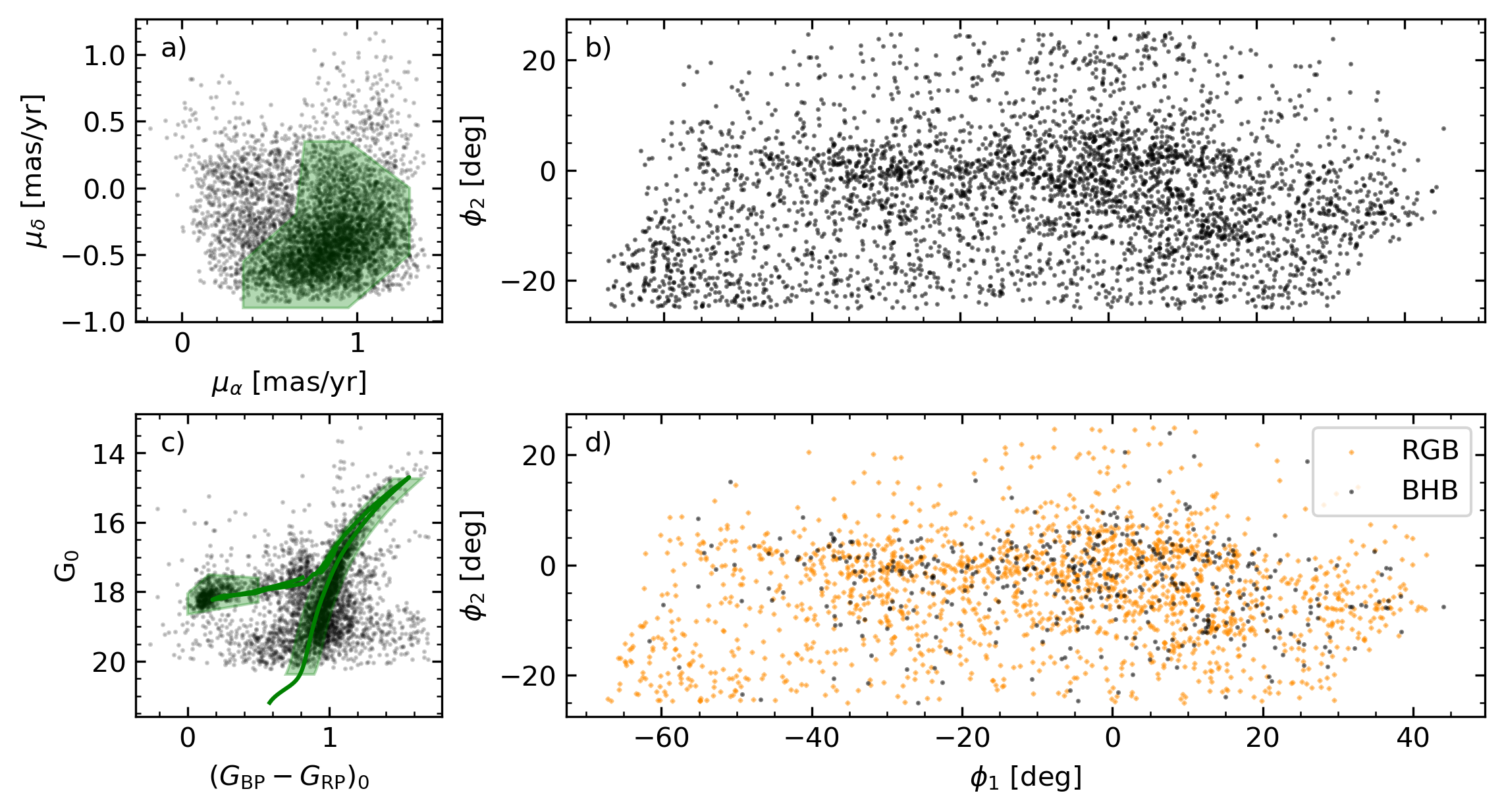
Figure 1: Initial selection of CPS members from the catalog of TB22. a) ICRS proper motions of 5336 stars with $P_{\rm{Cetus}}>0.5$ and $|\phi_{2}|\leq 25^{\circ}$. Stars belonging to the stream form an overdensity in proper motion space, which we select with the shaded polygon. b) On-sky positions of 3921 stars within the proper motion selection polygon in panel a in the CPS stream’s natural coordinates (see Section 3.1). c) Color-magnitude diagram of proper motion - selected stars. We use a 14 Gyr isochrone with [Fe/H] $=-1.93$ and shifted by a distance modulus of 17.7 (green line) to select BHB and RGB stars within the shaded regions. d) On-sky positions of 2210 stars passing both the proper motion and color-magnitude diagram selections. BHB (RGB) stars are shown as black circles (orange diamonds).

TB22 Catalog: We begin with the CPS member catalog selected from Gaia (Gaia Collaboration et al., 2016) EDR3 (Gaia Collaboration et al., 2021) as described in Section 4.3 of TB22. For the full details of their selection, we refer the interested reader to TB22, but provide an abridged version here. The sample is selected on the basis of color ($-0.5\leq(G_{\rm{BP}}-G_{\rm{RP}})_{0}\leq 1.7$), parallax ($-0.4<\varpi<0.2$ mas), proximity to the CPS orbital plane, and proper motion. Note that their orbital plane and proper motion selections are based on a different coordinate system for the CPS than we adopt in this paper (see Section 3.1).

In addition to these criteria, TB22 developed a model (their Equation 4) for the probability $P_{\rm{Cetus}}$ that a star in the sample belongs to the CPS (as opposed to the foreground or background), based on the stars’ sky positions and proper motions. The bottom panel of their Figure 12 shows the sky positions of the stars in their catalog with $P_{\rm{Cetus}}>0.2$.

We note that TB22 performed this selection to maximize completeness for the purposes of estimating the CPS progenitor’s mass. However, a kinematic study of the stream such as the one presented here requires that we apply additional criteria to maximize purity. To begin, we remove stars with $P_{\rm{Cetus}}<0.5$ and $|\phi_{2}|>25^{\circ}$.

Proper Motion Selection: Figure 1 illustrates the next steps of the selection process. Panel a shows the proper motions of potential stream stars. An overdensity in proper-motion space is indicated by the shaded polygon, which we fit by eye to maximize the contrast between the stream and the background. Panel b shows the stars encompassed by the polygon in CPS coordinates. Already, the stream is apparent against the remaining contamination.

Color-Magnitude Diagram Selection: To further refine our selection, we use the color-magnitude diagram in panel c, which contains all of the proper motion - selected stars. TB22 found that the CPS is well-described by a 14 Gyr-old MIST (Choi et al., 2016; Dotter, 2016) isochrone with [Fe/H] = -1.93 and a distance modulus of 17.7. We identify the BHB and red giant branch (RGB), and select stars belonging to both evolutionary stages within the shaded areas associated with this isochrone. In panel d, we are left with a relatively pure sample of CPS stars when compared with the original TB22 catalog, though some contamination remains.

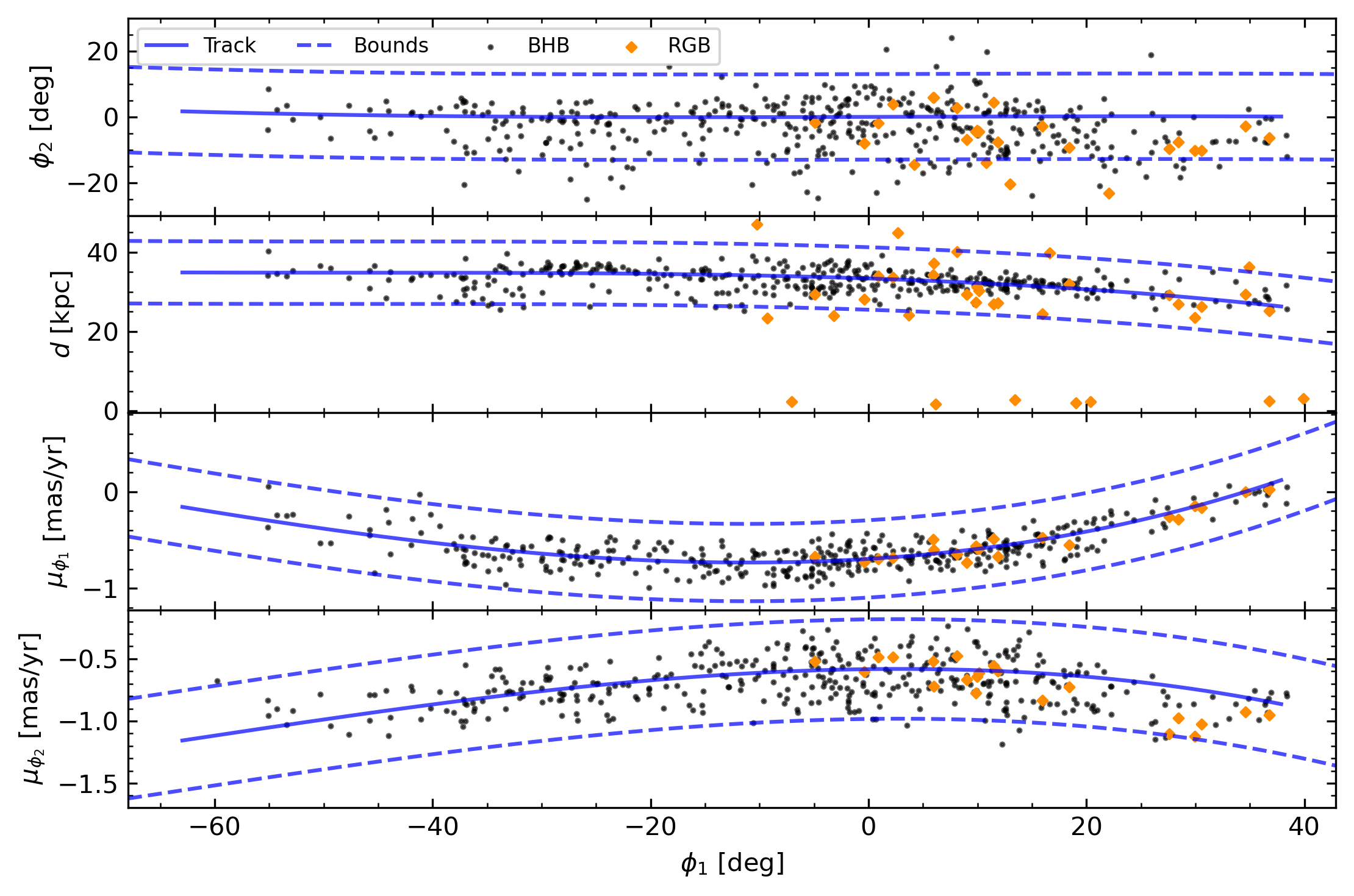
Figure 2: Track selection of 5-D CPS members. Each panel shows one phase-space coordinate ($\phi_{2}$, distance, proper motions) as a function of $\phi_{1}$. Black circles denote BHB stars selected in Figure 1, and orange diamonds show RGB stars selected in Figure 1 and cross-matched with H3. The solid lines show the Cetus-Palca-T21 track from galstreams (Mateu, 2023), and the dashed lines in each panel show the spread about the track used to select the stream as described in the text. Inspired by Koposov et al. (2019), Li et al. (2021), and Koposov et al. (2023), each panel contains stars selected from the other panels but not itself, i.e. stars in the $\phi_{2}$ panel are selected with distance and both proper motions, but not $\phi_{2}$. The final selection of stream members includes only stars that pass the selection in all four panels.

Radial Velocities and Distances: Thus far, our sample utilizes on sky positions and proper motions from Gaia. We now need distances and radial velocities for the stars in this sample to complete the full 6-dimensional dataset. To this end, we cross-match the remaining stars with the H3 survey (Conroy et al., 2019), identifying 47 matches from our RGB sample, and 8 matches from our BHB sample.

Performed with the MMT’s Hectochelle spectrograph (Szentgyorgyi et al., 2011), H3 consists of over 300,000 $\rm{R}=32,000$ spectra of MW halo stars selected from Gaia parallaxes and Pan-STARRS (Chambers et al., 2016) $r$-band magnitudes. H3 uses the MINESweeper pipeline (Cargile et al., 2020) to derive stellar parameters such as metallicities, $\alpha$-abundances, radial velocities, and spectrophotometric distances, and we use the latter two properties to fill in the remaining dimensions for our cross-matched CPS stars.

TB22 also identified 91 SEGUE (Yanny et al., 2009a) stars with spectroscopic radial velocities as likely CPS members, and we include a subset of 22 of these stars that meet the other selection criteria imposed so far. Distances for these SEGUE stars are provided by the machine-learning model presented in TB22. One star is duplicated in our SEGUE and H3 data, and we take the H3 values for its distance and radial velocity.

Next, to obtain distances for the BHB stars that were not matched with H3 or SEGUE, we make use of the Deason et al. (2011) relation between the color and absolute magnitude of BHB stars, re-calibrated for the Gaia EDR3 photometric system by TB22:

$$M_{\rm{G,BHB}}= -0.266(G_{\rm{BP}}-G_{\rm{RP}})_{0}^{3}+2.335(G_{\rm{BP}}-G_{\rm{RP}})_{0}^{2}$$ (1)

$$-1.955(G_{\rm{BP}}-G_{\rm{RP}})_{0}+0.794$$

Using this relation, we derive photometric distances to every BHB star in our remaining sample. Relative distance errors are assumed to be 5% (Deason et al. 2011; TB22). As no corresponding relation exists for RGB stars, we keep only the RGB stars that have distances measured from H3 (or from TB22’s model for the SEGUE stars).

Stream Track Selection: In Figure 2, we plot the BHB stars and RGB stars with known distances alongside the Cetus-Palca-T21 CPS track from galstreams. As a last step to increase the purity of our sample of 5-D stars, we remove stars far from this known stream track, similar to the method used by Koposov et al. (2023). The dashed blue lines show the region used to select stream stars in each dimension. We keep stars within $13^{\circ}$ of the $\phi_{2}$ track, 7.87 kpc of the distance track (the same width as the $\phi_{2}$ selection assuming a distance of 35 kpc), and 0.4 mas/yr of the proper motion tracks. These bounds are designed to fully encompass the stream given recent estimates of its 1-$\sigma$ width ($\sim$ $5^{\circ}$, $\sim$ $0.2$ mas/yr; TB22; Yuan et al. 2022) while discarding contaminants that are far from the stream track in position and/or velocity.

As in Figure 2 of Koposov et al. (2019), Figure 2 of Li et al. (2021), and Figure 1 of Koposov et al. (2023), each panel of Figure 2 shows the stars selected using constraints placed on the other three dimensions. For example, the stars shown in the top panel ($\phi_{2}$ versus $\phi_{1}$) are selected using the distance and proper motion cuts but not $\phi_{2}$. This allows us to confirm that our sample is relatively pure, i.e. no more than $11\%$ of stars in any given dimension lie outside our chosen bounds while passing the selections made in the other dimensions. Ultimately, we keep the stars that lie within the chosen bounds of the track in all four dimensions.

3.3 Radial Velocity Track

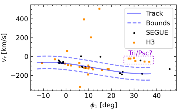
Figure 3: $v_{r}$ vs. $\phi_{1}$ for 55 stars with measured radial velocities after the selection process described in Section 3.2. SEGUE (H3) stars are shown as black circles (orange squares). The CPS is clearly visible in radial velocity space between $-12^{\circ}\lesssim\phi_{1}\lesssim 38^{\circ}$. In addition to the CPS, we identify a group of stars around $\phi_{1}\sim 33^{\circ}$ and $v_{r}\sim-20$ km/s that have radial velocities consistent with the Tri/Psc stream (purple box; see Section 6.3), as well as some contamination from stars clearly not associated with either stream. As described in the text, we fit a radial velocity track to the CPS stars (solid blue line), and keep the 39 stars within 66.4 km/s of this track (dashed blue lines) as members of our 6-D sample.

With our catalog of CPS members in-hand, we now turn to the subset of these members with measured radial velocities to determine the radial velocity track of the CPS. Figure 3 shows the heliocentric radial velocities ($v_{r}$) of the stars for which we have radial velocity measurements. While the CPS is clearly visible in radial velocity space, we see another group of stars near $\phi_{1}\sim 33^{\circ}$ and $v_{r}\sim-20$ km/s (inside the purple box). These stars have radial velocities consistent with the Triangulum / Pisces stream (Tri/Psc; Bonaca et al. 2012; Martin et al. 2013, 2014), which has a tentative association with the CPS (Bonaca et al. 2021; TB22; Yuan et al. 2022). We discuss these stars further in Section 6.3.

After removing the candidate Tri/Psc stars, we are left with CPS stars and a small number of contaminants. To find the radial velocity track of the CPS, we calculate the median $v_{r}$ in $10^{\circ}$ wide $\phi_{1}$ bins, shifted by $5^{\circ}$ along the stream, and then fit a third-degree polynomial to the binned medians. The result is shown as the solid blue line in Figure 3. To remove the remaining contaminants, we use the same method as in Figure 2, keeping stars with radial velocities less than 66.4 km/s from the track (dashed blue lines). This velocity limit of 66.4 km/s corresponds to 0.4 mas/yr in proper motion space assuming a distance of 35 kpc, consistent with the proper motion cuts in Figure 2.

Ultimately, we are left with a catalog containing two samples of CPS stars:

• 5-D Sample: 364 stars with five phase-space dimensions measured: sky positions, proper motions, and distances.

• 6-D Sample: 39 stars with all six phase-space dimensions measured via the addition of spectroscopic radial velocities.

These stars span $\sim 90^{\circ}$ on the sky at roughly constant $\alpha\sim 30^{\circ}$ between $\delta\sim-60^{\circ}$ - $+30^{\circ}$. The stream shows a distance gradient of 7 kpc, from $\sim 35$ kpc at the trailing edge to $\sim 28$ kpc at the leading edge, in agreement with the pure sample of BHB stars identified by TB22. These stream properties are also consistent with the previous detections of this wrap by Yuan et al. (2019) and Yuan et al. (2022). Note that we do not search for the diffuse component of the stream found in the Galactic north by Yuan et al. (2019) and Yuan et al. (2022), nor for the additional wraps identified by Yuan et al. (2022), as these are far from Segue 2 and are not expected to be recently affected by its passage.

4 Stream Orbit Fitting

In this section we estimate the orbit of the CPS based on the 5- and 6-D member catalogs assembled in the previous section. This allows us to track the location of the CPS stars backwards in time and identify the location and timing of closest approach between Segue 2 and the CPS. In Section 4.1, we describe our model of a combined MW / LMC gravitational potential. As no remnant of the CPS progenitor has been conclusively identified (e.g. Yuan et al. 2019, 2022; Chang et al. 2020; TB22), we utilize two complementary methods for inferring the stream’s orbit from the kinematics of its stars. In Section 4.2, we fit the orbit of the CPS based on a maximum-likelihood method used by Price-Whelan & Bonaca (2018) and Bonaca & Price-Whelan (2024), and in Section 4.3, we use the method of Chang et al. (2020) to find a stellar tracer that is representative of the stream. We refer to the orbits inferred with these methods as the “Fit Orbit” and “Tracer Orbit,” respectively.

4.1 Galaxy Models

Table 1: Galaxy model parameters.

Parameter	Value	Unit
Milky Way
$M_{\mathrm{vir}}$	$1\times 10^{12}$	$M_{\odot}$
$R_{\mathrm{vir}}$	262.76	kpc
$c_{\mathrm{vir}}$	9.86	-
$M_{\mathrm{disk}}$	$6.5\times 10^{10}$	$M_{\odot}$
$R_{\mathrm{disk}}$	3.5	kpc
$z_{\mathrm{disk}}$	0.53	kpc
$M_{\mathrm{H,bulge}}$	$1\times 10^{10}$	$M_{\odot}$
$a_{\mathrm{bulge}}$	0.7	kpc
LMC
$M_{\mathrm{H}}$	$1.8\times 10^{11}$	$M_{\odot}$
$a$	20	kpc

To find the orbit of the CPS, we require an assumption of the underlying gravitational potential. The MW model we adopt is described in Patel et al. (2017) and Patel et al. (2020) (their MW1). It is composed of an analytic NFW halo (Navarro et al., 1996b), a Miyamoto-Nagai disk (Miyamoto & Nagai, 1975), and a Hernquist bulge (Hernquist, 1990). We also include the LMC, owing to its substantial influence on the orbits of MW halo tracers (e.g. review by Vasiliev, 2023a, and references therein), such as stellar streams (e.g. Vera-Ciro & Helmi, 2013; Gómez et al., 2015; Erkal et al., 2018, 2019; Shipp et al., 2019, 2021; Ji et al., 2021; Vasiliev et al., 2021; Koposov et al., 2023; Lilleengen et al., 2023). Our LMC model is described in Garavito-Camargo et al. (2019) (their LMC3), and consists of an analytic Hernquist halo. The parameters of these galaxy models are summarized in Table 1.

The LMC’s primary effect on stellar streams stems from the reflex motion of the MW about the combined MW/LMC barycenter (e.g. Weinberg, 1995; Gómez et al., 2015; Erkal et al., 2019; Petersen & Peñarrubia, 2020; Ji et al., 2021; Vasiliev et al., 2021). We account for this by allowing the centers of mass of the MW and LMC to move in response to each other. However, as the potentials are analytic and therefore remain rigid and symmetric, we do not take into account the shape distortions of the MW and LMC halos during the LMC’s infall (Erkal et al., 2019; Garavito-Camargo et al., 2019; Cunningham et al., 2020; Erkal et al., 2020; Petersen & Peñarrubia, 2020; Garavito-Camargo et al., 2021; Makarov et al., 2023; Vasiliev, 2023b; Chandra et al., 2024; Sheng et al., 2024; Yaaqib et al., 2024). The consequences of this choice are discussed further in Section 6.2.2. We use the values given in Kallivayalil et al. (2013) for the LMC’s present-day Galactocentric position and velocity vector.

4.2 Likelihood Model

To fit the orbit of the CPS, we construct a maximum-likelihood-based model similar to the one used by Price-Whelan & Bonaca (2018) and Bonaca & Price-Whelan (2024), which searches for the orbit of a test particle that best traces the track of the stream. The Cetus-Palca-T21 track from galstreams is missing radial velocity information and is not informed by orbit fitting (Mateu, 2023). In contrast, a fit orbit will describe the stream more completely and will also be consistent with the potentials described in the previous section.

We note that, especially near apocenter, the track of a stream does not necessarily trace the stream orbit accurately, which can lead to additional systematic errors in fitting the MW potential if this assumption is made (Eyre & Binney, 2009, 2011; Sanders & Binney, 2013a, b). However, our aim is not to fit the potential of the MW / LMC system; rather we seek a description of the stream’s location as a function of time within a few hundred Myr of the present. Additionally, Chang et al. (2020) found that the CPS traces the orbit of its progenitor over the past $\sim$ two wraps. Therefore, finding the orbit that best traces the stream track is sufficient for our purposes.

In detail, we first initialize a test particle at a stream longitude of $\phi_{1,0}=45^{\circ}$, with the other phase-space coordinates given as model parameters:

$$\boldsymbol{P}=[\phi_{2,0},\>d_{0},\>\mu_{\alpha,0},\>\mu_{\delta,0},\>v_{r,0}].$$ (2)

Using gala, we integrate the test particle’s orbit backwards in time for 500 Myr in our combined MW/LMC potential. When interpolated with a cubic spline, this test particle orbit gives us a model of the stream’s “dependent” phase-space coordinates as a function of $\phi_{1}$ and $\boldsymbol{P}$:

$$\boldsymbol{\mathcal{O}}(\phi_{1},\boldsymbol{P})= [\phi_{2}^{orbit}(\phi_{1}),\>d^{orbit}(\phi_{1}),\>\mu_{\alpha}^{orbit}(\phi_{1}),\>$$ (3)

$$\mu_{\delta}^{orbit}(\phi_{1}),\>v_{r}^{orbit}(\phi_{1})].$$

We calculate the log-likelihood that the test particle orbit passes through the stream based on the measured locations of the CPS stars selected in Section 3:

$$\rm{ln}(\mathcal{L})=\sum_{i}\sum_{j}\left(-\frac{1}{2}\frac{(\mathcal{O}_{i}(\phi_{1,j},\boldsymbol{P})-x_{ij})^{2}}{\delta x_{ij}^{2}}-\frac{1}{2}\rm{ln}(2\pi\,\delta x_{ij}^{2})\right),$$ (4)

where the subscript $i$ labels the five dependent coordinates such that the position of the $j$th star is ($\phi_{1,j}$, $x_{ij}$), and $\delta x_{ij}$ similarly denotes the uncertainty on the $j$th star’s position in the $i$th coordinate. The uncertainties we use for this calculation are as follows.

For the $\phi_{2}$ uncertainties, the width of the stream in $\phi_{2}$ is on the order of degrees, much larger than the Gaia astrometry errors which are typically less than a milliarcsecond. This makes the observational errors a poor estimate of the uncertainty in the orbit given the width of the stream. Instead, we measure the $1\sigma$ width of the stream in $\phi_{2}$ (denoted $\sigma_{\phi_{2}}$) and set $\delta\phi_{2}$ equal to this for every star. To calculate $\sigma_{\phi_{2}}$, we first find the standard deviation of the star positions in $\phi_{2}$ in a $10^{\circ}$-wide $\phi_{1}$ window shifted by $5^{\circ}$ along the stream. After verifying the width of the stream is approximately constant with $\phi_{1}$ (see the solid line in the top row of panels in Figure 13), we set $\sigma_{\phi_{2}}$ equal to the mean of the binned widths, which is $4.8^{\circ}$. This width is consistent with other recent estimates of the CPS’s width (TB22; Yuan et al. 2022).

The distance uncertainties are those reported by SEGUE or H3 where available, or assumed to be 5% for the BHB photometric distances (Deason et al. 2011; TB22), as discussed in Section 3.2. We keep the proper motions in equatorial coordinates (as opposed to CPS coordinates) so that we can use the reported errors from Gaia without needing to transform these to the CPS frame. For stars with measured radial velocities, we use the uncertainties reported by SEGUE or H3. For stars without measured radial velocities, we use a value of 0 km/s and an uncertainty of 1000 km/s to ensure that these stars do not meaningfully contribute to the likelihood in the $v_{r}$ dimension.

To find the maximum of the likelihood, we use the BFGS algorithm available in scipy.optimize (Virtanen et al., 2020).

4.3 Representative Tracer Star

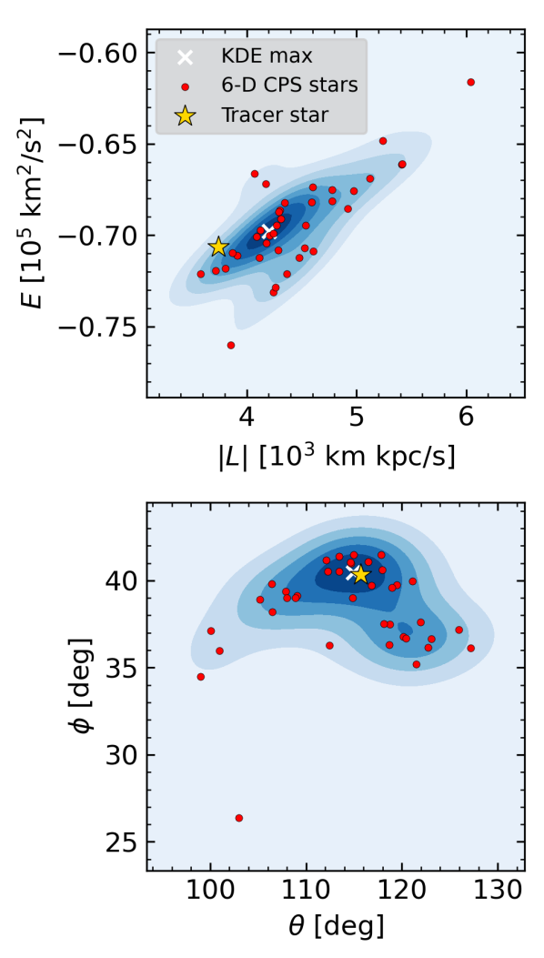
Figure 4: Selection of a 6-D star with an orbit representative of the stream. The distribution of 6-D stars in energy-angular momentum (top panel) and orbital pole (bottom panel) spaces is shown by the red points and as contours of a kernel density estimate (KDE). The max of the KDE in each panel is shown with a white cross. The “representative” star selected as the stream tracer (yellow star) is close to the max of the orbital pole distribution and below the max of the $(E,|\boldsymbol{L}|)$ distribution (c.f. Figure 3 of Chang et al. (2020)).

For a complementary method of estimating the orbit of the CPS, we use a slight modification of the method presented in Chang et al. (2020) to identify a single tracer star whose orbit is representative of the rest of the stream. For each star in our 6-D sample, we calculate the orbital energy $E$ and orbital angular momentum $\boldsymbol{L}$ about the MW’s center of mass in Galactocentric coordinates. From the angular momentum, we also calculate the stars’ orbital poles ($\theta$, $\phi$), where $\theta=\rm{arccos}(L_{z}/|\boldsymbol{L}|)$ is the polar angle from the Galactocentric $z$-axis, and $\phi=\rm{arctan2}(L_{x},|\boldsymbol{L}|)$ is the azimuthal angle from the Galactocentric $x$-axis.

Similar to Figure 3 of Chang et al. (2020), Figure 4 shows the distribution of the 6-D stars in the ($E$, $|\boldsymbol{L}|$) and ($\theta$, $\phi$) spaces in the top and bottom panels, respectively. For each space, we construct a kernel density estimate (KDE) of the distribution, shown by the shaded contours. To choose a representative tracer star, we sum the values of the two KDEs (normalized such their maxima are equal to 1) at the position of each star and choose the star with the largest combined value. The chosen tracer (yellow star) is very close the maximum of the orbital pole distribution (white cross) and below the maximum of the ($E$, $|\boldsymbol{L}|$) distribution.

4.4 Orbits

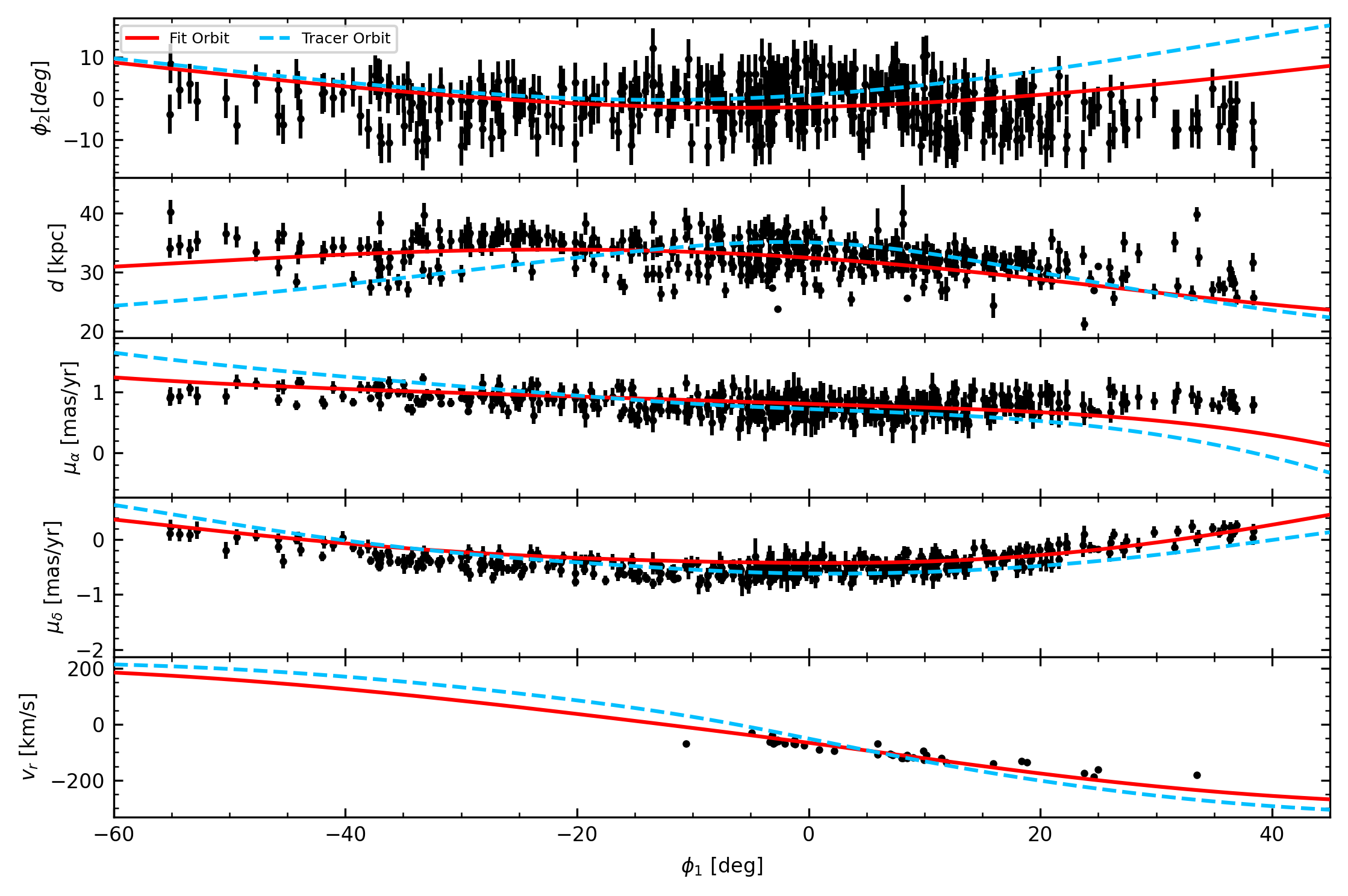
Figure 5: Model orbits for the CPS. Each panel shows the positions of the stars and their associated errors in the phase-space coordinates used to fit the CPS orbit as described in Section 4.2, plotted against $\phi_{1}$. Note that the top four panels show all of the stars in our CPS catalog, while the $v_{r}$ panel (bottom) shows only the 6-D sample for clarity. The orbit of the test particle with initial conditions that maximize Equation 4 is shown as the solid red line (“Fit Orbit"), while the orbit of the representative star found in Section 4.3 is shown as the dashed blue line (“Tracer Orbit"). The Fit Orbit traces the stream’s location over nearly its entire length. The Tracer Orbit reproduces the overall behavior of the stream but fits less well than the Fit Orbit.

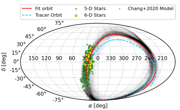
Figure 6: Sky positions in Mollweide projection of our CPS stars and orbit models compared to the CPS N-body model presented in Chang et al. (2020). Our CPS stars are split into the 5-D sample (green circles) and 6-D sample (yellow diamonds). The Fit and Tracer Orbits are shown as the solid red and dashed blue lines, respectively. The CPS model from Chang et al. (2020) is shown as the black points in the background. Our CPS member stars and orbits agree very well with the Chang et al. (2020) model, though the Tracer Orbit deviates slightly from the model in the North.

The CPS orbits derived from the methods described in Sections 4.2 and 4.3 are presented in Figure 5. Note that the proper motions are given in equatorial coordinates while the other dimensions are in CPS coordinates, as in Equation 4. Both orbits are integrated 500 Myr forwards and 500 Myr backwards from their initial conditions. For the “Fit CPS Orbit,” (solid red line) the initial conditions are those which maximize Equation 4, while the “Tracer CPS Orbit” (dashed blue line) is integrated from the present-day position and velocity of the tracer star. Note that the bottom panel ($v_{r}$ vs. $\phi_{1}$) shows only stars with measured radial velocities for clarity. In this panel, the radial velocity errorbars are typically smaller than the points.

The Fit Orbit traces the location of the stream well, lying within the width of the stream over its entire length in every dimension except $\mu_{\alpha}$, in which the orbit diverges from the stream slightly at $\phi_{1}>25^{\circ}$. The best agreement between the stream and orbit is in the region where the radial velocity data is concentrated, roughly $-5^{\circ}<\phi_{1}<15^{\circ}$. The Tracer Orbit tracks the stream less well when compared to the Fit Orbit. As the CPS is a dwarf galaxy stream, it is relatively hot and we may expect that a single star may not accurately trace the entire stream, as seen here. However, the Tracer Orbit still broadly agrees with the shape of the stream, and fits quite well in the $-5^{\circ}<\phi_{1}<15^{\circ}$ region where radial velocity information is available.

As another check on our stream member selection and orbits, we compare our results to the N-body simulation of the CPS presented in Chang et al. (2020), the present-day snapshot of which is made publicly available in Yuan et al. (2022). While this simulation does not include the LMC, Chang et al. (2020) argue the LMC has a negligible effect on the past orbit of the CPS progenitor. Figure 6 shows their present-day snapshot along with our member catalog and orbits on-sky. Our Fit Orbit agrees very well with the Chang et al. (2020) model, matching the position of the simulated stream over a full wrap. Our Tracer Orbit matches the simulation well in the South, but differs from the simulation by $\sim 10^{\circ}$ in the North. The Fit (Tracer) orbit has an apocenter of $\sim 38$ (39) kpc and a pericenter of $\sim 20$ (16) kpc, which is also in broad agreement with the Chang et al. (2020) model and the orbits of individual CPS BHB stars in TB22.

Altogether, we are confident that our Fit Orbit is an appropriate model of the stream over the most recent wrap, while the Tracer Orbit provides an example of how individual stars move with respect to the overall stream track. Differences between these two orbits illustrate the uncertainties in modeling the stream, and will allow us to compare two different Segue 2 / CPS impact geometries moving forward in Section 5.

5 Interaction with Segue 2

With the orbit of the CPS determined, we now seek to characterize the stream’s interaction with Segue 2. To study whether Segue 2 had a close passage with the CPS, we use gala to compute the orbit of Segue 2 from its present-day position and velocity in our combined MW/LMC potential (see Section 4.1).

Table 2: Summary of Segue 2’s present-day position and velocity.

Parameter	Value	Unit	Reference
$\alpha$	34.8167	deg	1
$\delta$	20.1753	deg	1
Dist. modulus	17.7$\pm$0.1	mag	1,2
$\mu_{\alpha}$	1.47$\pm$0.04	mas/yr	3
$\mu_{\delta}$	-0.31$\pm$0.04	mas/yr	3
$v_{r}$	-39.2$\pm 2.5$	km/s	1,2

Segue 2’s present-day 6-D phase space information is derived from the combination of radial velocity, distance modulus, and proper motions. We adopt the R.A., Dec., distance modulus, and heliocentric radial velocity from McConnachie & Venn (2020a), and the proper motions from McConnachie & Venn (2020b), who compute proper motions of MW satellites using Gaia EDR3. Note that the distance and radial velocity of Segue 2 were first reported in Belokurov et al. (2009). To account for uncertainties in the present-day 3-D position and velocity vectors of Segue 2, we consider 2000 Monte-Carlo (MC) draws from the joint 1-$\sigma$ error space of Segue 2’s distance, proper motion, and radial velocity. These values are summarized in Table 2. From each MC draw, we derive Segue 2’s 6-D phase-space vector in Galactocentric Cartesian coordinates before integrating its orbit. Our fiducial Segue 2 orbit is its “direct orbital history,” computed by taking the Table 2 values without errors.

5.1 The Close Approach Between Segue 2 and the CPS

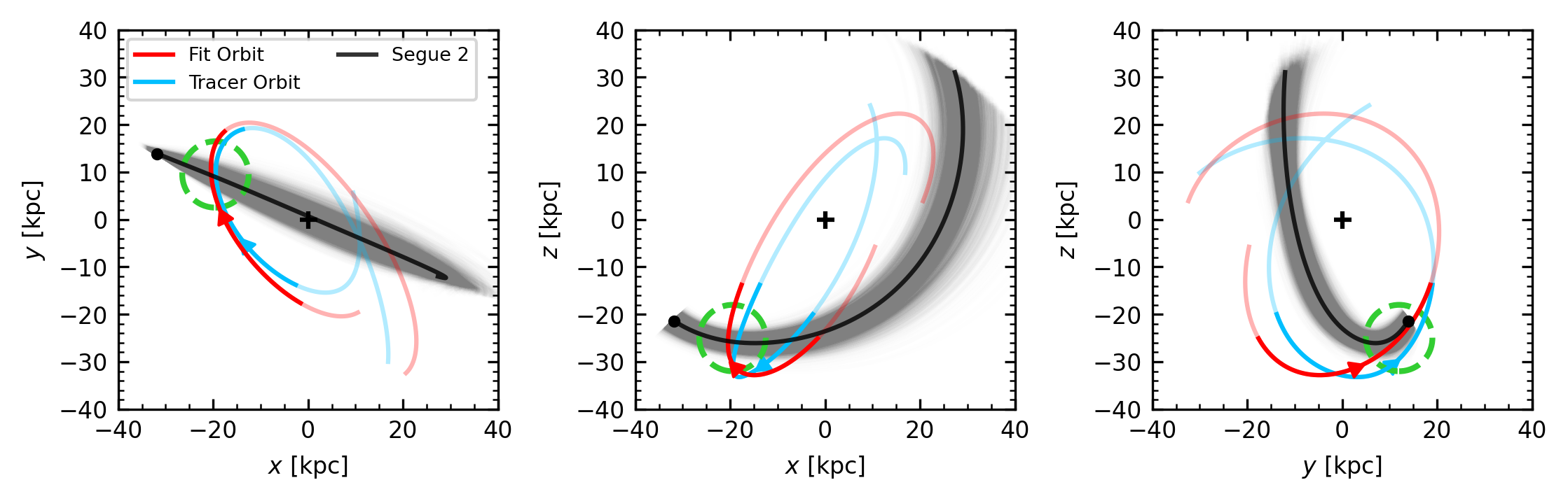
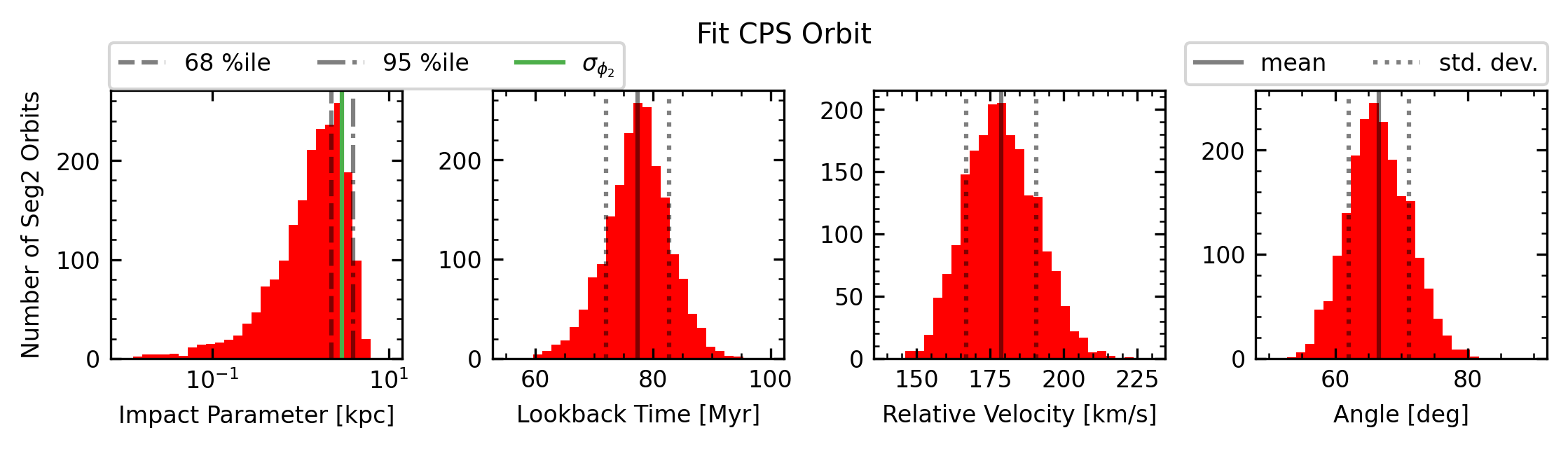
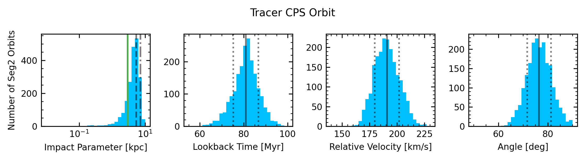
Figure 7: Galactocentric projections of our model stream orbits and Segue 2’s orbit. Each panel shows a different projection, with the Galactic center marked by the cross. Our Fit CPS Orbit and Tracer CPS Orbit are shown as the red and blue lines, respectively. The bold sections of the stream orbits mark the portion that is covered by our member star catalog, and arrows denote the stream’s direction of motion along the orbit. The present-day location of Segue 2 is marked by the black dot, and the black line shows its fiducial orbit over the past 500 Myr. The remainder of the Monte-Carlo Segue 2 orbits (as described in the text) are shown with gray lines. Segue 2 has a recent, close approach with the CPS, the approximate location of which is marked with a dashed circle in each panel.

Figure 8: Distributions of the timings and geometry of the recent flyby encounter between the MC Segue 2 and our model orbits. The top (bottom) row of panels shows the orbit parameters at closest approach to the Fit CPS Orbit (Tracer CPS Orbit). From left-to-right, each row contains histograms of: the impact parameter or closest approach distance, lookback time or how far in the past the closest approach occurred, the relative velocity between Segue 2 and the stream test particle at the point of closest approach, and the angle between the Segue 2 orbits and the CPS orbit. A solid green line in the impact parameter panels denotes the 1$\sigma$ radius of the stream, while dashed and dot-dashed lines indicate the 68th and 95th percentile, respectively, of the Segue 2 orbits. The solid and dotted vertical lines in the other panels show the mean and standard deviation of the distributions. See Table 3 for a summary of these values. Every Segue 2 orbit passes within 10 kpc of both model CPS orbits within 56-100 Myr ago.

Table 3: Summary of parameters describing the flyby between Segue 2 and the CPS.

Parameter	Measured w/	Measured w/	Unit
	Fit Orbit	Tracer Orbit
MC Segue 2 Orbits
Med. Impact P.	1.54	4.59	kpc
% Seg2 $<$ 1$\sigma_{\phi_{2}}$	82.00	17.34	-
% Seg2 $<$ 2$\sigma_{\phi_{2}}$	99.90	77.16	-
Lookback Time	$77.4\pm 5.4$	$81.0\pm 5.7$	Myr
Rel. Velocity	$178.6\pm 11.9$	$190.8\pm 11.1$	km/s
Angle	$66.6\pm 4.6$	$76.5\pm 4.8$	deg
Fiducial Segue 2 Orbit
Impact P.	1.36	4.67	kpc
Lookback Time	77.8	81.2	Myr
Rel. Velocity	178.3	190.4	km/s
Angle	66.6	76.6	deg

Figure 8 shows the distribution of MC Segue 2 orbits (grey lines) with the fiducial present-day location and orbit of Segue 2 (black dot and line) highlighted. Each Segue 2 orbit has been integrated backwards in time for 500 Myr. The proper motion uncertainties are responsible for a $\sim 10^{\circ}$ spread in Segue 2’s orbital plane, while the distance uncertainties drive a $\sim 10$ kpc spread in its pericenter distance. We also plot the model CPS orbits presented in Section 4.4, with the Fit and Tracer Orbits shown as the red and blue line respectively. For each CPS orbit, we highlight the section of the orbit between $-56^{\circ}<\phi_{1}<38^{\circ}$ where our catalog of member stars is located. Arrows at arbitrary locations denote the direction the stream stars move along the orbits.

All of the possible Segue 2 orbits pass close to the CPS orbits within the longitude range covered by stream stars (the flyby location is highlighted by a dashed green circle in each panel), implying that Segue 2 had a recent close flyby with the observable portion of the CPS. To more precisely quantify the probability, timing, and geometry of the flyby, we calculate the minimum distance (impact parameter) between each MC Segue 2 orbit and both model CPS orbits. At each point of closest approach, we determine how far in the past the closest approach occurred (lookback time), the relative velocity between Segue 2 and the model CPS orbit’s test particle at the time of closest approach, and the angle that Segue 2’s trajectory makes with the stream orbit.

The distributions of these quantities are plotted in Figure 8. Each panel shows a histogram of one quantity for all of the 2000 MC Segue 2 orbits, measured with respect to one of the CPS model orbits. The top row is calculated with the Fit CPS Orbit, while the bottom row is calculated with the Tracer CPS Orbit. For lookback time, relative velocity, and angle, we include solid and dotted lines denoting the mean and standard deviation of the distribution. Numerical values of these statistics are provided in Table 3 along with the corresponding values for the fiducial Segue 2 orbit.

For the impact parameters, the distributions are folded at zero (as negative impact parameters are impossible), so simply calculating and reporting the mean and standard deviation are not appropriate. Instead, we estimate the probability that Segue 2 has an impact parameter inside the stream as follows: We use $\sigma_{\phi_{2}}=2.92$ kpc (the angular width of the stream in $\phi_{2}$ as described in Section 4.2, converted to a length assuming a distance of 35 kpc) as an estimate for the width of the stream. The solid green line in the left column of panels denotes $\sigma_{\phi_{2}}$, while the dashed and dot-dashed lines in the impact parameter panels show the 68th and 95th percentile of the impact parameters. In our analysis, we consider impact parameters within $2\sigma_{\phi_{2}}=5.84$ kpc to be “direct hits,” i.e. Segue 2’s center of mass passes within the radius from the stream’s orbit that contains approximately 95% of the stream stars. Table 3 reports the percentage of Segue 2 orbits with impact parameters less than $\sigma_{\phi_{2}}$ and $2\sigma_{\phi_{2}}$.

The median impact parameter is 1.54 kpc for the Fit Orbit, and 4.59 kpc for the Tracer Orbit. All but two of the 2000 possible Segue 2 orbits pass within $2\sigma_{\phi_{2}}$ of the Fit CPS Orbit, while only $77.16\%$ pass within $2\sigma_{\phi_{2}}$ of the Tracer CPS Orbit. This discrepancy is caused by the difference in the position of the model CPS orbits around $\phi_{1}\sim 10^{\circ}$ where the flyby occurs (see Section 5.2). In this region, the Tracer Orbit is at a larger distance and closer to the upper edge of the stream in $\phi_{2}$, slightly farther away from the fiducial Segue 2 orbit, which passes just inside the Fit Orbit (see Figure 8).

The timing of the encounter is consistent between the stream orbit models and is roughly 80 Myr ago, while the relative velocity of the flyby differs at just over 1-$\sigma$, with the Fit Orbit implying a $\sim 10$ km/s lower velocity ($\sim$180 km/s) than the Tracer Orbit ($\sim$190 km/s).

Segue 2’s orbital plane is inclined $\sim 40^{\circ}$ to that of the CPS. As Segue 2 crosses the stream, it moves from the interior of the stream’s orbit to the exterior, making a total angle of $\sim 67^{\circ}$ with the Fit CPS Orbit, and $\sim 76^{\circ}$ with the Tracer CPS Orbit. These differences in impact angle are barely more than 2-$\sigma$, and are again driven by the Tracer Orbit being slightly less parallel to the stream stars in the vicinity of the flyby.

In summary, we find that when considering the observational errors on Segue 2’s distance and velocity vector, Segue 2 has a high probability (99.9% or 77.16% depending on the stream model) of directly impacting the CPS between 60-100 Myr ago.

5.2 Perturbation Predictions

Table 4: Summary of our Segue 2 models

Model	Profile	Total Mass	Scale Radius
		[$10^{9}M_{\odot}$]	[kpc]
Seg2-1P	Plummer	0.5	0.686
Seg2-2P	Plummer	1.0	0.865
Seg2-3P	Plummer	5.0	1.48
Seg2-3H	Hernquist	5.0	8.35
Seg2-4P	Plummer	10.0	1.86

In this section, we quantify the expected perturbation to the CPS due to Segue 2’s close passage as a function of Segue 2’s mass and density profile. The Segue 2 models used in this section are summarized in Table 4. As motivated in Section 5, these Segue 2 models are chosen to represent a range of possible formation scenarios for Segue 2, including tidally truncated halos of varying mass (represented by Plummer potentials) and a massive intact halo (represented with a Hernquist potential). For each choice of profile and total mass, we fit the scale radius such that the mass enclosed within a radius of 46 pc is $1.5\times 10^{5}M_{\odot}$, consistent with the upper limit on Segue 2’s dynamical mass within its half-light radius by Kirby et al. (2013). Throughout this section, we use Segue 2’s fiducial orbit, i.e. the black line in Figure 8, unless otherwise noted. As a reminder, the lower portion of Table 3 lists the impact geometry for this orbit.

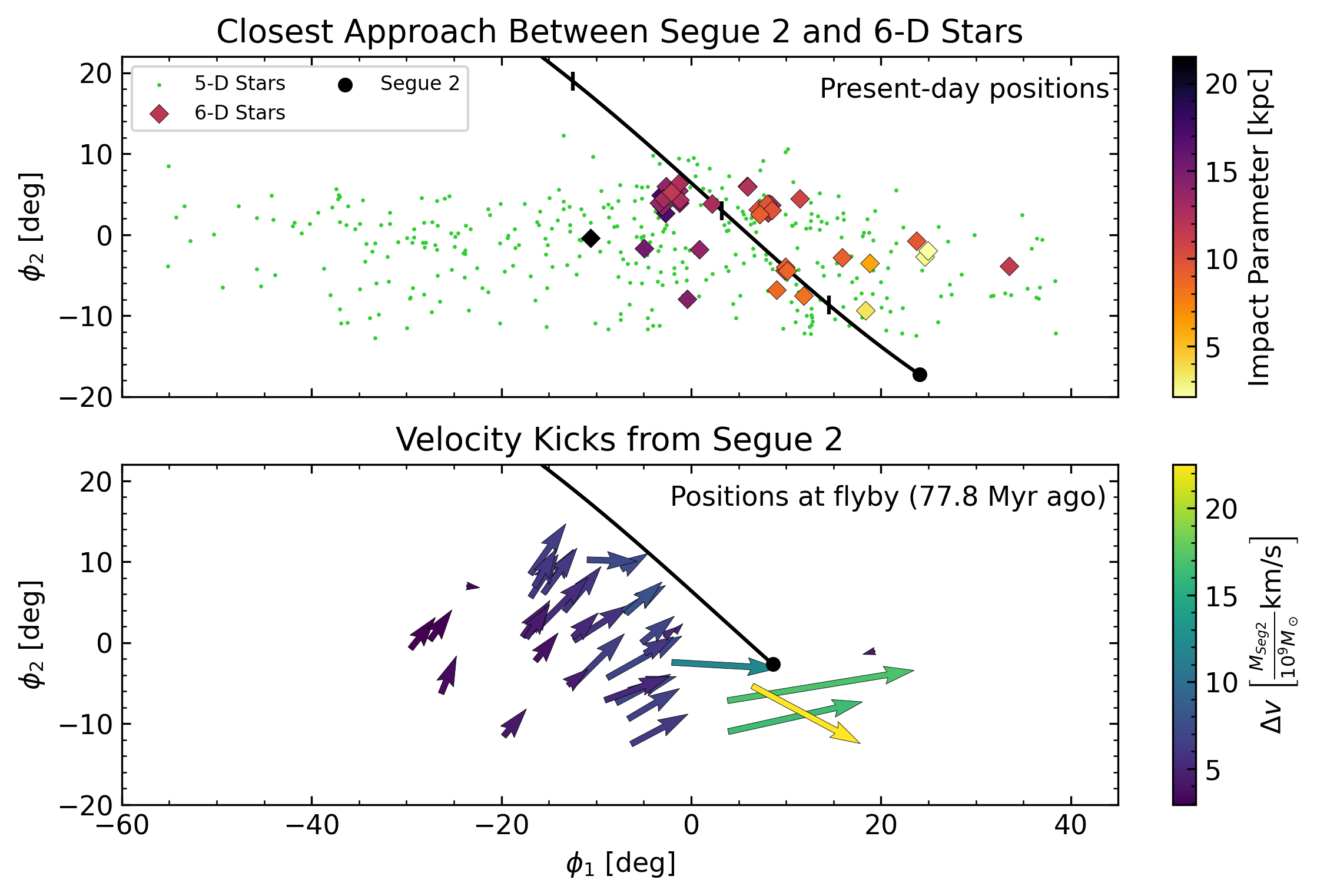
Figure 9: Geometry of the perturbation imparted on 6-D CPS stars from a $10^{9}\,M_{\odot}$ Segue 2. The top panel shows the present-day locations of the 5-D stars (green points), 6-D stars (colored diamonds), Segue 2 (black point), and its fiducial orbit over the past 500 Myr (black line). Tick marks along Segue 2’s orbit denote 50 Myr increments. 6-D star points are colored according to their minimum distance (impact parameter) to Segue 2 over the past 500 Myr. The bottom panel shows the same at the time of closest approach with the Fit CPS Orbit (77.8 Myr ago), omitting the 5-D stars as their positions at this time are not known. Arrows drawn from the 6-D stars’ positions indicate the projected direction and magnitude of the change in velocity of each star due to Segue 2. Segue 2 passes through the leading edge of our 6-D star sample, pulling stars near the flyby location primarily in the direction of their orbits, while deflecting the trailing portion of the stream slightly to the west.

To begin, we integrate our 6-D CPS stars backwards in time for 500 Myr, adding the influence of our $10^{9}\,M_{\odot}$ Plummer Seg2-2P model such that the stars feel gravity from the MW, LMC, and Segue 2. For each star, we measure the closest approach / impact parameter between the star and Segue 2, as well as the change in the star’s velocity due to Segue 2 (i.e. the difference in the star’s velocity with and without Segue 2’s gravity). The latter measurement is taken by numerically integrating over the star’s acceleration from Segue 2 over the duration of the simulation. The results are plotted in Figure 9. The top panel shows the locations of the 6-D stars and Segue 2 at the present day. We also include the 5-D stars for a reference of the position of the stream as a whole. The 6-D stars are colored by their impact parameter with respect to Segue 2. The stars around $\phi_{1}\sim 25^{\circ}$ (similar to Segue 2’s present longitude) have the smallest impact parameters of $\sim 2.5$ kpc, and are expected to be the most perturbed by Segue 2’s passage.

To show where the 6-D stars are relative to Segue 2 during the encounter, the bottom panel is drawn 77.8 Myr ago when Segue 2 has its closest approach with the Fit CPS Orbit. In this panel, we only include the 6-D stars (as the 5-D stars cannot be integrated backwards owing to their missing radial velocities). The 6-D stars are represented as arrows which point from the stars’ positions and denote the magnitude and projected direction of their change in velocity due to Segue 2, based on integrating their accelerations from Segue 2 over the past 500 Myr. Assuming Segue 2 has a mass of $10^{9}\,M_{\odot}$, it changes the velocities of stars near the flyby by $\sim 20$ km/s, comparable to the overall velocity dispersion of the stream. As the stars’ accelerations due to Segue 2 are directly proportional to Segue 2’s mass, the largest velocity perturbation received by a star from the Plummer models scales as $\Delta v_{\rm{max}}\sim(22.5\,\rm{km/s})(M_{\rm{Seg2}}/10^{9}M_{\odot})$, and similarly for the other stars. From this basic test, we can already see that it is likely that Segue 2 masses above $10^{9}\,M_{\odot}$ are required to measurably increase the velocity dispersion of the CPS, which we confirm in Section 5.3.1.

From the top panel of Figure 9, there are many 5-D stars in the vicinity of the largest perturbation / smallest impact parameter at present. Unfortunately, the stars for which we have spectroscopic data only cover one side of the flyby well, as only one of our 6-D stars is ahead of Segue 2 at the time of flyby (bottom panel).

The limited radial velocity data precludes a detailed search for Segue 2’s effect on the stream with our 6-D observational data. However, the existing data does provide strong motivation that limits on Segue 2’s mass profile can be made with future radial velocity datasets such as e.g. DESI (Cooper et al. 2023; see Sections 5.3.1 & 5.3.2). Instead, we turn to constructing a set of synthetic stream models to predict the signatures of Segue 2’s flyby in the CPS as function of Segue 2’s mass and density profile. These models are described in Section 5.3, and the results are presented in Sections 5.3.1 (mass) and 5.3.2 (density profile).

5.3 Synthetic Streams

We note that the most detailed modeling strategy for the CPS would self-consistently generate a model stream by simulating the disruption a dwarf galaxy through particle-spray methods or an N-body simulation as in e.g., Chang et al. (2020). Such an approach is expensive, however, especially when considering the need to fine-tune the initial conditions of the simulation to globally reproduce the observed properties of the stream. These difficulties are compounded by the fact that the CPS progenitor’s location is unknown. Here, our goal is simply to compare the perturbations generated by different Segue 2 mass models on a local area of the stream. Therefore, we utilize a much less expensive strategy which involves distributing star particles along our stream orbits from Section 4.4 according to the measured width of the stream in each dimension.

In detail, we use both of our interpolated CPS orbits as “templates” for the synthetic streams that describe the streams’ positions in $\phi_{2}$, $d$, $v_{r}$, $\mu_{\phi_{1}}$, and $\mu_{\phi_{2}}$ as a function of $\phi_{1}$ similarly to Section 4.2. For each synthetic stream, we distribute 1000 star particles uniformly in $\phi_{1}\in[-80,70]$, with the other five phase-space coordinates specified by the template orbit. This results in a linear density of stars similar to the most dense portion of the observed stream.

We then introduce a scatter in the star particles’ phase-space positions, drawing the scatter in each coordinate from an independent normal distribution. The width of the distribution in each dimension is as follows: The spread in $\phi_{2}$ is $\sigma_{\phi_{2}}$. The scatter in each proper motion direction is estimated with the same procedure as $\sigma_{\phi_{2}}$ (see Section 4.2), i.e. we calculate the binned standard deviation of the stream in $\mu_{\phi_{2}}$ and then take the mean of the binned widths. In principle, the width of the observed stream already encodes perturbations from Segue 2, but as only a portion of the stream is near the impact site, averaging over longitude bins reduces the contribution of the perturbed portion to the width measurement. The spread in $d$ ($v_{r}$) is the same as the spread in $\phi_{2}$ $(\mu_{\phi_{2}}$), translated to a length (linear velocity) using the distance of the template orbit at the $\phi_{1}$ location of each star. This process generates a population of stars that locally reproduces the observed properties of the CPS, suitable for estimating Segue 2’s influence on the stream.

5.3.1 The Mass of Segue 2

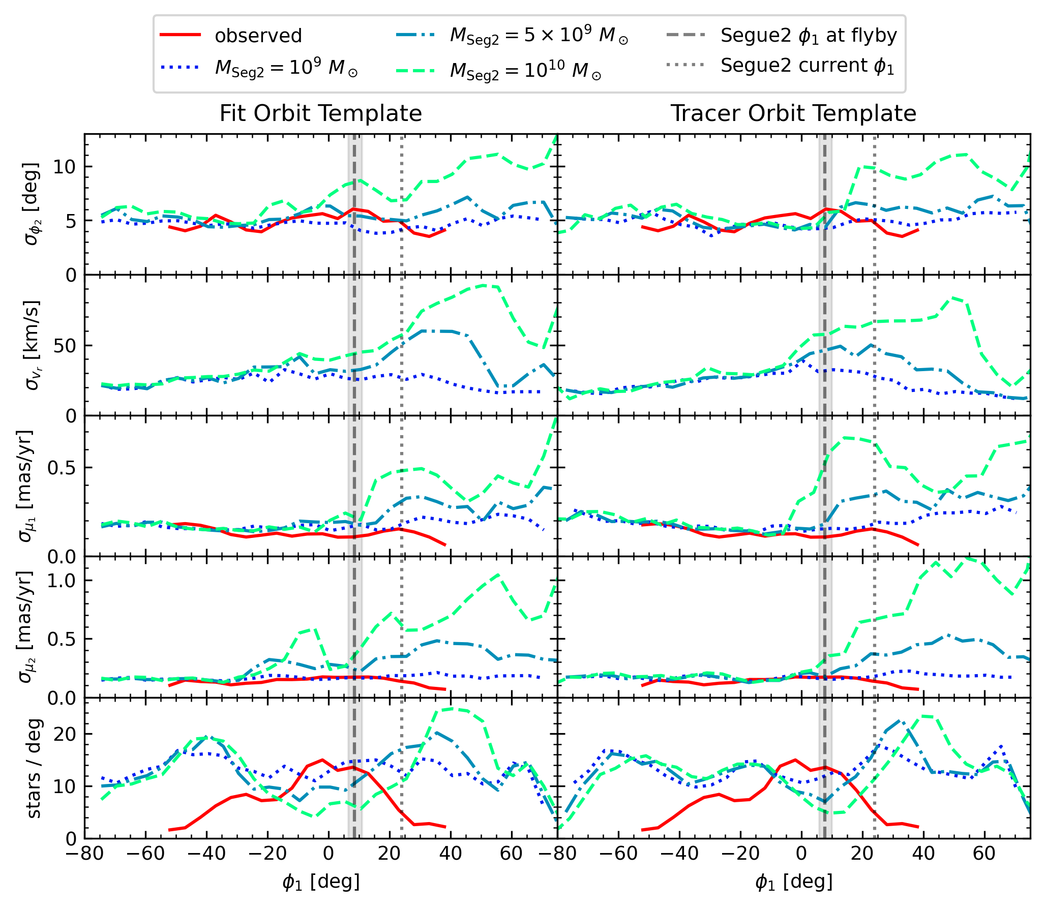
Figure 10: Width and density of our synthetic streams as a function of $\phi_{1}$ and Segue 2’s mass. The left column of panels shows the streams generated from the Fit Orbit, while the right column shows streams generated from the Tracer Orbit. Each panel shows the width of the observed stream (solid red line), and perturbed models (dotted, dash-dotted, and dashed lines) in one dimension, with the bottom row showing the linear density of the streams. The streams perturbed by a $10^{9}$ $M_{\odot}$ Segue 2 are effectively identical to the $5\times 10^{8}$ $M_{\odot}$ and unperturbed cases, so we omit the latter two for clarity. Note that we do not include the observed radial velocity width of the CPS as we have too few stars with measured radial velocities to plot a width reliably along the full length of the stream. For reference, vertical dotted lines indicate the present-day $\phi_{1}$ location of Segue 2, and vertical dashed lines show the location of closest approach of the fiducial Segue 2 orbit to the stream orbit. A shaded region shows the spread of the flyby locations from the 2000 MC Segue 2 orbits described in Section 5.1. A significant perturbation (larger than the shot noise from placing the stars) to the CPS is expected if Segue 2 has a mass $>10^{9}M_{\odot}$. A Segue 2 mass of $10^{10}\,M_{\odot}$ is inconsistent with the observed properties of the CPS.

Once the synthetic streams are generated, we integrate the star particles backwards in time for 500 Myr in the gravity of the MW and LMC only. At this point, we inject Segue 2 on its fiducial orbit and integrate forward to the present day, allowing the stars to feel the gravity of all three galaxies. To quantify the heating of the stream by Segue 2, we measure the dispersion of the stream in $\phi_{2}$ and its three velocity components in a series of $10^{\circ}$ - wide $\phi_{1}$ bins, shifted by $5^{\circ}$ along the stream. In addition, we measure the linear density of the stream by counting the number of stars in each bin.

We repeat this process for each of the synthetic stream templates (CPS orbits) and each of the Plummer Segue 2 models in Table 4. The results for the streams generated from the Fit and Tracer Orbits are shown in the left and right columns of Figure 10, respectively. For comparison, we also include the width / density of the observed CPS in every dimension except radial velocity dispersion, as we do not have enough stars with spectroscopic radial velocities to accurately measure this quantity. To guide the eye, a dashed vertical line in each panel denotes the $\phi_{1}$ location of the fiducial Segue 2 orbit’s closest approach to the stream orbit, while the shaded region shows the 5 - 95 percentile range of the MC Segue 2 flyby locations. Similarly, a dotted vertical line shows the present-day $\phi_{1}$ location of Segue 2. Note that we omit the $M_{\rm{Seg2}}=5\times 10^{8}\,M_{\odot}$ case and the unperturbed synthetic stream for clarity, as these are effectively identical to the $M_{\rm{Seg2}}=10^{9}\,M_{\odot}$ case (dotted lines).

In other words, if Segue 2’s mass is $\leq 10^{9}\,M_{\odot}$, it does not leave a detectable perturbation signature in the dispersions of the stream stars. This agrees with the result in Section 5.2 that the velocity kicks imparted to stream stars by a $10^{9}\,M_{\odot}$ Segue 2 are comparable to the intrinsic dispersion of the stream.

Conversely, if Segue 2 has a mass of $5\times 10^{9}\,M_{\odot}$, its passage noticeably heats the stars in the vicinity of the flyby. By the present day, the proper motion (radial velocity) dispersion of the stream near Segue 2’s present-day location ($\phi_{1}\approx 25^{\circ}$) is $\sim 0.15$ mas/yr (40 km/s) higher than the unperturbed portion of the stream. In the $M_{\rm{Seg2}}=10^{10}\,M_{\odot}$ case, the heating is even larger, $\sim 0.3$ mas/yr in proper motions or $\sim$ 50 km/s in radial velocity in the vicinity of Segue 2.

Interestingly, a $10^{10}\,M_{\odot}$ Segue 2 also noticeably heats the stream behind the flyby location. In particular, the $\mu_{\phi_{2}}$ dispersion of the stream based on the Fit Orbit is $\sim 0.3$ mas/yr higher around $\phi_{1}\sim-10^{\circ}$ in response to a $10^{10}\,M_{\odot}$ Segue 2 than the other masses we consider. A similar bump in the $\mu_{\phi_{1}}$ dispersion near $\phi_{1}\sim 0^{\circ}$ can be seen in the stream based on the Tracer Orbit in the presence of a $10^{10}\,M_{\odot}$ Segue 2. This heating of the CPS behind the flyby is inconsistent with the observed CPS.

Direct comparisons between the simulated and observed velocity dispersions at $\phi_{1}\gtrsim 10^{\circ}$ (the impact site) are challenging as the density of the CPS drops quickly with increasing $\phi_{1}$ (bottom panels of Figure 13). The series of cuts we employed in the construction of the catalog (Section 3) may exclude stream stars that have experienced large velocity kicks from Segue 2, which may artificially drop the CPS density in this region.

Alternatively, the drop in density may be a genuine gap caused by Segue 2’s passage. To investigate this possibility, we compare the observed decrease in density to the simulated streams (bottom panels of Figure 13). A $10^{9}\,M_{\odot}$ Segue 2 does not cause significant variations in the density of our synthetic streams above the shot noise from placing the star particles. For higher Segue 2 masses however, the beginning stages of gap formation can be seen in the form of an underdensity around $\phi_{1}\sim 0^{\circ}$ and corresponding overdensity around $\phi_{1}\sim 30^{\circ}$. This effect is mild in the case of a $5\times 10^{9}\,M_{\odot}$ Segue 2. However, if Segue 2 has a mass of $10^{10}\,M_{\odot}$, the significant underdensity in the simulated streams at $\phi_{1}\sim 0^{\circ}$ is inconsistent with the observed CPS’s density peak at this location.

Running all three simulations into the future reveals that a gap in the stream due to Segue 2’s flyby forms $\sim 300$, 200, or 70 Myr in the future if Segue 2’s mass is $10^{9}$, $5\times 10^{9}$, or $10^{10}\,M_{\odot}$, respectively. Even the earliest allowed flyby given the uncertainties in Segue 2’s distance and proper motion is no more than 100 Myr ago (see Figure 8), less than 23 Myr earlier than the fiducial Segue 2 orbit we simulate here. Therefore, even the earliest allowable flyby of the most massive Segue 2 model we consider leaves insufficient time for gap formation before the present day.

Instead, we see three potential causes of the observed drop in density at the leading edge of the stream:

1. Incompleteness and/or crowding in the observations in this region as the stream approaches the MW’s disk.

2. Intrinsic variations in the density of the stream due to the details of its formation process (e.g., epicyclic density variations; Küpper et al. 2008, 2010, 2012; Just et al. 2009; Mastrobuono-Battisti et al. 2012).

3. Selection effects from our catalog construction process (see Section 3). If the stream is indeed heated by Segue 2 at $\phi_{1}\gtrsim 10^{\circ}$, a flat proper motion cut such as the one employed here would select fewer stars in the heated portion of the stream.

Future work will be needed to determine the contribution of each effect.

To summarize, we find that a Segue 2 mass as high as $10^{10}\,M_{\odot}$ produces high-level inconsistencies between the observed and simulated properties of the stream. We cannot confidently rule out a mass of $5\times 10^{9}M_{\odot}$ given the outstanding uncertainties in the observations and the inherent limitations of our simplistic modeling approach. If Segue 2’s mass is $\leq 10^{9}\,M_{\odot}$, we should not expect to observe heating in the CPS due to the interaction at present. None of the Segue 2 models or orbits we consider are capable of creating a density gap in the CPS by the present day. The primary effect of a sufficiently massive Segue 2’s passage at present is heating of the stream in all three velocity components at $\phi_{1}\gtrsim 10^{\circ}$.

5.3.2 The Density Profile of Segue 2

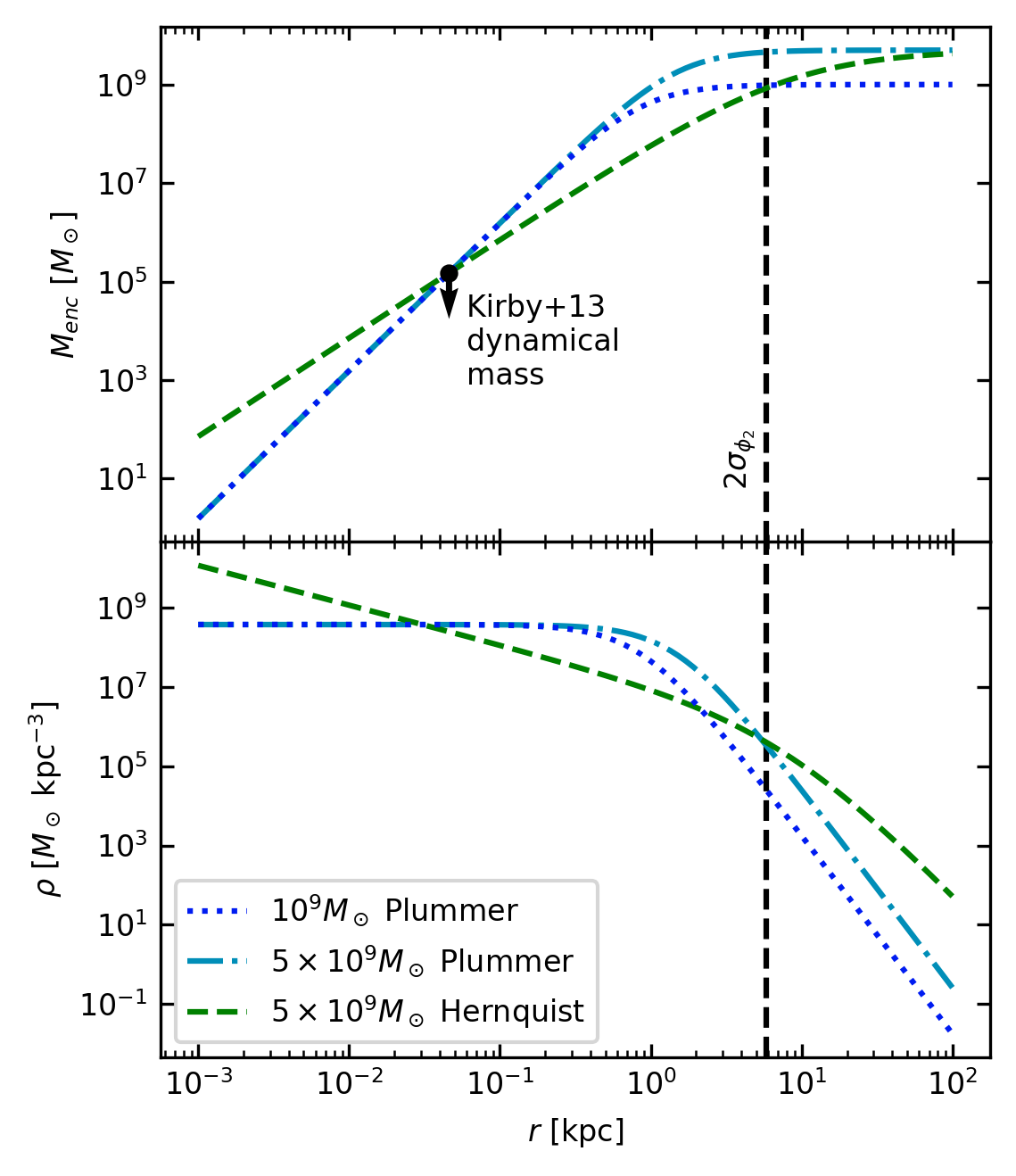
Figure 11: Mass (top) and density (bottom) profiles for the Segue 2 models studied in Section 5.3.2. The $10^{9}\,M_{\odot}$ and $5\times 10^{9}\,M_{\odot}$ Plummer profiles are shown as the dotted and dash-dotted lines, while the $5\times 10^{9}\,M_{\odot}$ Hernquist profile is shown as the dashed line. All profiles match the Kirby et al. (2013) dynamical mass limit for Segue 2 by construction. A vertical dashed line indicates the 2-$\sigma$ width of the CPS, which marks the radius from Segue 2’s center that the stream is sensitive to Segue 2’s mass as explained in the text.

Here, we investigate the possibility of using the Segue 2 / CPS interaction to constrain the density profile of Segue 2’s DM halo. As a basic test, we compare our Plummer sphere models to a Hernquist sphere with a total mass of $5\times 10^{9}\,M_{\odot}$. (see Section 5.3.1 & Table 4). We choose this mass as it is above the threshold where the CPS is sensitive to Segue 2’s passage in Figure 13, allowing us to compare the effects of a cuspy (Hernquist) vs. cored (Plummer) profile. Note that in addition to having a central core, a Plummer profile falls off more steeply than a Hernquist profile outside of its scale radius, and is therefore a better approximation of a tidally truncated halo. For reference, we plot the mass and density profiles of the $10^{9}\,M_{\odot}$ and $5\times 10^{9}\,M_{\odot}$ Plummer profiles and the $5\times 10^{9}\,M_{\odot}$ Hernquist profile in Figure 11. As a reminder, the enclosed mass of all profiles is $1.5\times 10^{5}\,M_{\odot}$ at a radius of 46 pc (Kirby et al. 2013; black circle) by construction.

The Hernquist model for Segue 2 leaves no detectable perturbation in the width or density of either synthetic stream by the present day. In other words, if we were to plot the properties of the synthetic stream perturbed by the Hernquist Segue 2 model on Figure 10, it would look extremely similar to the synthetic stream perturbed by the $M_{\rm{Seg2}}=10^{9}\,M_{\odot}$ Plummer sphere Segue 2 model.

This can be understood in terms of the mass enclosed by each Segue 2 model within its impact parameter to the stream stars, which determines the gravitational acceleration felt by the stars for a fixed Segue 2 orbit. Depending on Segue 2’s impact parameter to the stream’s orbit, the encounters allowed by the MC Segue 2 orbits (see Figure 8) can be split into two cases:

• Direct hits (impact parameters in (0, $2\sigma_{\phi_{2}}\approx 6$] kpc): In this case, Segue 2’s center of mass passes within the stream. Individual stream stars will therefore have impact parameters with respect to Segue 2 spanning the width of the stream, i.e. within (0, $2\sigma_{\phi_{2}}$].

• Close flybys (impact parameters between 6 - 10 kpc; note that no Segue 2 orbits allowed within the error space have impact parameters larger than 10 kpc): In this case, some individual stream stars will still pass within $2\sigma_{\phi_{2}}$ of Segue 2’s center of mass, because Segue 2 cannot be more than $10-5.84=4.16$ kpc from the edge of the stream.

Therefore, within the range of impact parameters to the CPS orbit allowed by Segue 2, individual stream stars will probe Segue 2’s mass within roughly $2\sigma_{\phi_{2}}\approx 6$ kpc. In Figure 11, we mark $2\sigma_{\phi_{2}}$ with a dashed, vertical line. Note that within this distance, the enclosed mass of the $10^{9}\,M_{\odot}$ Plummer profile is very similar to the $5\times 10^{9}\,M_{\odot}$ Hernquist profile, explaining why both models have the same effect on the width of our synthetic streams.

This allows us to refine our conclusions from the previous section about Segue 2’s mass profile. Namely, any Segue 2 DM density profile that encloses a total mass $\leq 10^{9}M_{\odot}$ within $\sim 6$ kpc is not expected to leave a measurable perturbation on the CPS. On the other hand, if a perturbation is detected, this would put a lower limit on Segue 2’s mass within $\sim 6$ kpc of $>10^{9}M_{\odot}$.

Crucially, the Segue 2 / CPS interaction is unique in that the perturbing DM halo hosts a luminous galaxy that has a dynamical mass estimate within $\sim$ 50 pc. When combined with a mass measurement at kiloparsec scales from our predicted stream perturbation, these two data points will measure the slope of Segue 2’s density profile.

For the sake of a strong example, let us pretend that a future observation with a well-characterized selection function has searched for and discovered a hot component of the CPS ahead of the impact site which is consistent with our predictions for a $5\times 10^{9}\,M_{\odot}$ Plummer sphere (i.e. Segue 2’s mass is $5\times 10^{9}\,M_{\odot}$ within $\sim 6$ kpc). In this hypothetical case, to simultaneously satisfy both this constraint and the Kirby et al. (2013) dynamical mass constraint at 46 pc, Segue 2’s density profile could not fall off more steeply than approximately $r^{-0.86}$ over this range, which would exclude an NFW or Hernquist profile, though not a DM cusp. In short, Segue 2’s interaction with the CPS may be capable of providing a second data point on the mass profile of a UFD at a drastically different distance scale than is probed by its internal dynamics.

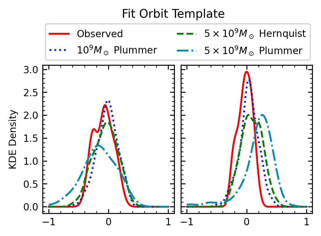
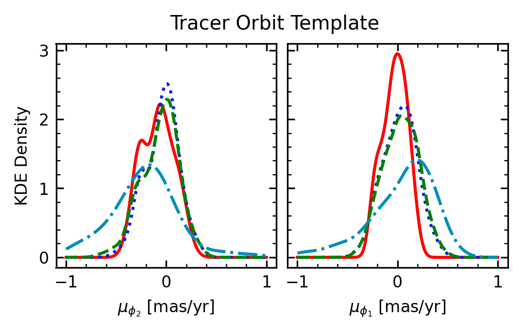
Figure 12: Proper motion distributions of the stars within $10^{\circ}<\phi_{1}<30^{\circ}$ (the impact site). The top (bottom) row shows the synthetic streams generated from the Fit (Tracer) Orbit, as well as the observed CPS stars. In both cases, the synthetic stream perturbed by a $10^{9}\,M_{\odot}$ Plummer Segue 2 is similar to the observed stream. The $5\times 10^{9}\,M_{\odot}$ Plummer Segue 2 broadens the tails of the distributions in both components, and shifts the peak of the distribution by roughly $-0.2$ mas/yr in $\mu_{\phi_{1}}$ and $0.2$ mas/yr in $\mu_{\phi_{2}}$. For the Tracer Orbit synthetic streams, the $5\times 10^{9}\,M_{\odot}$ Hernquist case is similar to the $10^{9}\,M_{\odot}$ Plummer case. However, for the Fit Orbit synthetic streams, the $5\times 10^{9}\,M_{\odot}$ Hernquist Segue 2 creates subtle shoulders in the distributions around $\mu_{\phi_{2}}\sim-0.3$ and $\mu_{\phi_{1}}\sim 0.2$ which are not created by the $10^{9}\,M_{\odot}$ Plummer profile. The velocity distribution of stars near the impact site can distinguish between Segue 2 mass profiles, with the existing data slightly preferring a $10^{9}\,M_{\odot}$ Plummer sphere.

We next examine the impact of changes in Segue 2’s DM density profile on the velocity distribution of CPS stars. We plot KDEs of the proper motion distributions of stars near the impact location ($\phi_{1}\in(10^{\circ},30^{\circ})$) for the observed CPS and the synthetic streams perturbed by our Seg2-2P, Seg2-3P, and Seg2-3H Segue 2 models (those shown in Figure 11) in Figure 12. In this figure, the proper motions of the synthetic stream stars are shown with respect to the orbit template used to generate the synthetic stream, while the observed proper motions are shown with respect to the Cetus-Palca-T21 track. The $5\times 10^{9}\,M_{\odot}$ Plummer model for Segue 2 has the largest effect on the velocity distributions, broadening the tails and shifting the peak of the distribution up (down) by about 0.2 mas/yr in $\mu_{\phi_{1}}$ ($\mu_{\phi_{2}}$). This shifting of the proper motion distributions suggests that a sufficiently massive Segue 2 may be capable of creating a track / velocity misalignment near the impact, as has been seen in other streams due to the LMC (e.g. Erkal et al., 2018; Koposov et al., 2019; Erkal et al., 2019; Ji et al., 2021; Shipp et al., 2021; Vasiliev et al., 2021; Koposov et al., 2023).

The $5\times 10^{9}\,M_{\odot}$ Hernquist and $10^{9}\,M_{\odot}$ Plummer models for Segue 2 do not affect the distributions as strongly, creating shoulders instead of shifting the entire distribution. For example, both of these models create a shoulder near $\mu_{\phi_{2}}\sim-0.3$ in the Tracer Orbit synthetic streams, which is also seen in the observed CPS. For the Fit Orbit synthetic streams (for which Segue 2’s impact parameter is smaller), the $5\times 10^{9}\,M_{\odot}$ Hernquist Segue 2 creates slight shoulders in the distributions around $\mu_{\phi_{2}}\sim-0.3$ and $\mu_{\phi_{1}}\sim 0.2$, while the $10^{9}\,M_{\odot}$ Plummer Segue 2 does not. To summarize, the velocity distribution of stars near the flyby location is mildly sensitive to the extended mass distribution of Segue 2, which could help break the degeneracy in stream heating between a $10^{9}\,M_{\odot}$ Plummer and $5\times 10^{9}\,M_{\odot}$ Hernquist profile. Breaking this degeneracy would provide insight on both the level of tidal stripping experienced by Segue 2 and whether DM cores can form in the absence of strong supernova feedback.

6 Discussion

6.1 Sensitivity of Our Results to Segue 2’s Orbit

As we have only considered Segue 2’s fiducial orbit in Sections 5.2 & 5.3, it is worth asking to what extent our results depend on Segue 2’s orbit. In Figure 10, we consider synthetic streams made with both CPS orbit models, which results in two different flyby distances, timings, velocities, and angles (see the bottom portion of Table 8). The heating in the CPS caused by Segue 2 is much more sensitive to changes in Segue 2’s mass (compare different lines within the same panel) than changes in the flyby (compare the same Segue 2 mass within a row).

Additionally, as the CPS is a thick stream, individual stream stars in a given flyby will have a range of impact parameters and relative velocities to Segue 2 that is similar to the range of impact parameters and relative velocities allowed by the uncertainty in Segue 2’s orbit. Therefore, we expect the magnitude of the perturbation in the CPS primarily probes Segue 2’s mass and is insensitive to Segue 2’s orbit within its allowed parameter space.

6.2 Limitations of Our Models

In this section, we discuss the outstanding limitations inherent in our choice of modeling approach. Specifically, we address: the effect of the MW and LMC masses in Section 6.2.1, our choice of rigid galaxy potentials in Section 6.2.2, and the effect of dynamical friction in Section 6.2.3.

6.2.1 MW and LMC mass

Table 5: Model parameters for our alternative potentials.

Parameter	Value	Unit
Heavy MW
$M_{\mathrm{vir}}$	$1.5\times 10^{12}$	$M_{\odot}$
$R_{\mathrm{vir}}$	300.79	kpc
$c_{\mathrm{vir}}$	9.56	-
$M_{\mathrm{disk}}$	$5.5\times 10^{10}$	$M_{\odot}$
$R_{\mathrm{disk}}$	3.5	kpc
$z_{\mathrm{disk}}$	0.53	kpc
$M_{\mathrm{H,bulge}}$	$1\times 10^{10}$	$M_{\odot}$
$a_{\mathrm{bulge}}$	0.7	kpc
Heavy LMC
$M_{\mathrm{H}}$	$2.5\times 10^{11}$	$M_{\odot}$
$a$	25.2	kpc

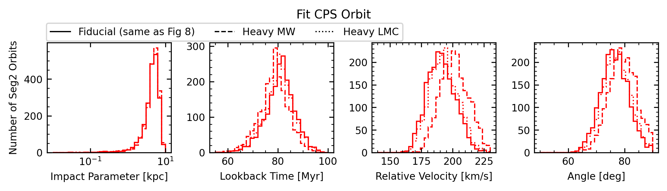
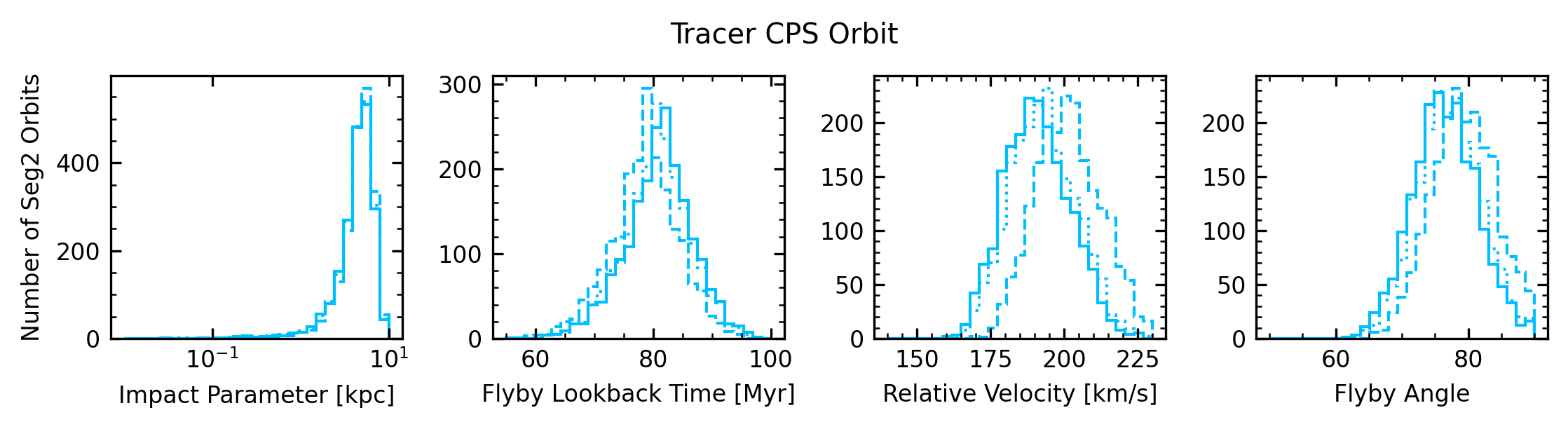
Figure 13: Same as Figure 8, with the addition of the flyby parameter distributions in our Heavy MW (dashed lines) and Heavy LMC potentials (dotted lines). The probability of a close encounter, i.e. distribution of impact parameters, is unchanged by modifying the MW or LMC mass. The timing, relative velocity, and angle of the flyby are negligibly affected by changing the LMC mass. Changing the MW mass does not affect the shape of the distributions, but causes the encounter to happen at smaller lookback times, at a slightly higher relative velocity and angle. Changes in the mean flyby timing, relative velocity, and angle owing to a larger MW mass are all $\approx$ 1$\sigma$.

Table 6: Flyby parameters in our alternative potentials.

Parameter	Measured w/	Measured w/	Unit
	Fit Orbit	Tracer Orbit
Heavy MW
Lookback Time	$74.9\pm 5.4$	$78.5\pm 5.7$	Myr
Rel. Velocity	$191.0\pm 12.1$	$201.5\pm 11.3$	km/s
Angle	$69.3\pm 4.4$	$79.2\pm 4.8$	deg
Heavy LMC
Lookback Time	$77.0\pm 5.4$	$80.6\pm 5.7$	Myr
Rel. Velocity	$181.4\pm 12.0$	$192.9\pm 11.2$	km/s
Angle	$67.4\pm 4.6$	$77.1\pm 4.8$	deg

To determine the dependence of our results on the mass of the MW and LMC, we repeat the analyses of Sections 4 and 5.1 with two alternative potentials, varying the mass of the Milky Way in one version and the mass of the LMC in the other. The model parameters for our Heavy MW and Heavy LMC are listed in Table 5. The Heavy MW is the same as the MW2 model from Patel et al. (2020), and the Heavy LMC is Garavito-Camargo et al. (2019)’s LMC4.

The results of this experiment are shown in Figure 13, which shows the distributions of flyby parameters for the 2000 MC Segue 2 orbits similarly to Figure 8. The solid lines reproduce the distributions from Figure 8 in our fiducial potential, while the dashed (dotted) lines show the distributions calculated with the Heavy MW (LMC). Looking at the left column of panels (impact parameter), it is clear that the probability of Segue 2’s flyby with the CPS is unchanged by varying the mass of the MW or LMC. In other words, the CPS / Segue 2 interaction is recent enough that changes in the orbits of both objects in our alternative mass models are too small to prevent the encounter. A more massive LMC or MW does not affect the shape of the timing, relative velocity, or flyby angle distributions. Instead, a heavier LMC causes the flybys to occur slightly more recently, at a larger relative velocity, and at larger angles, though these differences are negligible. A more massive MW causes the same effects, though the differences from the fiducial MW mass are more pronounced, at about the 1-$\sigma$ level. Table 6 contains a summary of the flyby timing and geometry in our alternative potentials.

6.2.2 Deformation of the MW and LMC

In this work, we have chosen to use rigid, spherical or axisymmetric potentials for all the galaxies we consider. While we account for the bulk movement / reflex motion of the MW’s center of mass in response to the LMC, our choice of rigid potentials fails to account for the shape and kinematic distortions to the halos of the MW and LMC owing to their interaction (Erkal et al., 2019, 2020, 2021; Garavito-Camargo et al., 2019; Cunningham et al., 2020; Petersen & Peñarrubia, 2020; Garavito-Camargo et al., 2021; Petersen & Peñarrubia, 2021; Makarov et al., 2023; Vasiliev, 2023b; Chandra et al., 2024; Sheng et al., 2024; Yaaqib et al., 2024).

However, the CPS is currently far from the LMC and orbits within the inner halo of the MW where the effects of the LMC are less prominent (e.g. Laporte et al., 2018; Erkal et al., 2019, 2020; Garavito-Camargo et al., 2019; Vasiliev, 2023a; Sheng et al., 2024). In addition, we have demonstrated that our results are insensitive to changing the mass of the MW or LMC (see Section 6.2.1), which will have a larger effect on the orbits of Segue 2 and the CPS than the detailed shape of the MW’s halo. In short, we do not expect the shape of the MW’s halo and/or presence of the LMC to change the fact that Segue 2 is impacting the CPS.

6.2.3 Dynamical Friction

In our simulations, we have neglected the effect of dynamical friction, which in general causes the orbits of objects within a host galaxy’s DM halo to decay over time (Chandrasekhar, 1943). To confirm that dynamical friction does not cause a significant change in the orbits of MW satellites over the timescales we consider in this work (the past 500 Myr), we compare the LMC’s orbit over this time in our simulations to an orbit with dynamical friction from Patel et al. (2020). Their orbit is computed in their MW1 potential (which we also use in this work; see Section 4.1). By 500 Myr, the LMC’s position in our simulation differs from that of Patel et al. (2020) by just $\approx 2$ kpc. Over the timescales in which Segue 2 interacts with the CPS (< 100 Myr ago), the LMC’s position in the two simulations is effectively identical. The strength of the dynamical friction drag force scales as $M_{\rm{sat}}/v_{\rm{sat}}^{2}$ (Chandrasekhar, 1943), so the drag force on our most massive Segue 2 model will be $\approx 3.6$ times weaker than the drag on the LMC at present. Therefore, neglecting dynamical friction in our simulations has no bearing on our results.

6.3 Triangulum / Pisces Stream Candidates

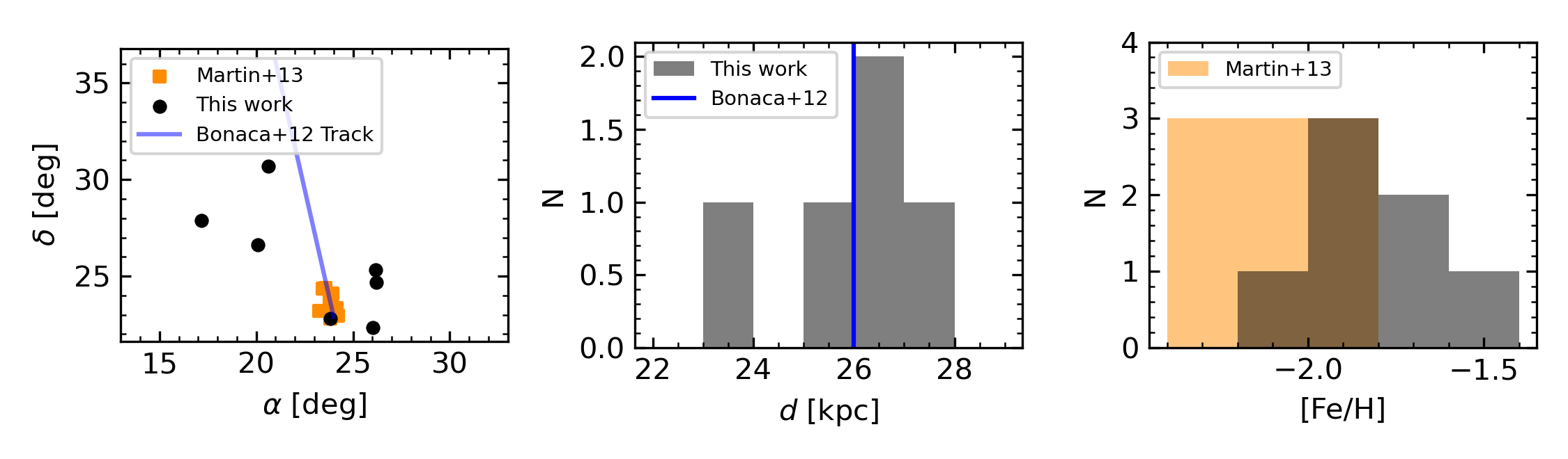
Figure 14: Comparison of our Tri/Psc candidates to the Tri-Pis-B12 track and the Martin et al. (2013) Tri/Psc catalog. The left panel shows the sky positions of our stars (black points), the Martin et al. (2013) stars (orange squares), and the Tri-Pis-B12 track (blue line). One of our stars is included in the Martin et al. (2013) sample. The remaining stars cluster around the track with a large spread. In the center panel, we show the distance distribution of our candidates. Bonaca et al. (2012) measured the distance of Tri/Psc to be 26 kpc (indicated by the blue line). The right panel compares the metallicity distribution of our candidates (black) to that of the Martin et al. (2013) stars (orange). While our candidates are spread out with respect to the stream track, they are consistent with Tri/Psc in spatial location, metallicity, and radial velocity (see Figure 3), suggesting they may correspond to an envelope or cocoon structure.

Here, we conduct a further investigation into the group of seven stars identified in the purple box in Figure 3 as having radial velocities and longitudes consistent with the Tri/Psc stream. Figure 14 compares the on-sky positions of these stars to the Tri-Pis-B12 track from Bonaca et al. (2012) published in galstreams and to a catalog of spectroscopic Tri/Psc members published by Martin et al. (2013). One of the Martin et al. (2013) stars is present in our candidate list. While the remaining six candidates are $\gtrsim 2^{\circ}$ from the stream track, their distances and metallicities are roughly consistent with constraints on Tri/Psc from Bonaca et al. (2012) and Martin et al. (2013) respectively.

Therefore, we tentatively propose that the six candidates not previously identified as Tri/Psc members may be part of a wider “cocoon” component of the stream, similar to those found around GD-1 (Malhan et al., 2019; Valluri et al., 2024) and Jhelum (Bonaca et al., 2019a; Awad et al., 2024). Such a hot envelope around Tri/Psc would be consistent with the picture that its globular cluster progenitor once belonged to the dwarf galaxy progenitor of the CPS as proposed by Bonaca et al. (2021) (see also TB22; Yuan et al. 2022). In this scenario, the hot envelope could be created via pre-processing of the globular cluster inside the Cetus-Palca dwarf (e.g. Carlberg, 2018) and could be used to constrain the density profile of the Cetus-Palca dwarf’s DM halo (e.g. Malhan et al., 2021). Additional study will be needed to confirm the association between these stars and the cold component of the stream.

7 Conclusions

In this paper, we have used the observed kinematics of the CPS and Segue 2 to discover and study the interaction between these two members of the MW halo. Our main findings are summarized below.

• Beginning with the catalog of TB22, we identify a relatively pure sample of 403 RGB and BHB stars belonging to the CPS. 39 of these stars have spectroscopic radial velocities measured with SEGUE or H3. Our sample is consistent with other detections of the main CPS wrap (Yuan et al., 2019, 2022). However, we refrain from searching for other components of the CPS identified by these authors.

• We employ two methods for inferring the orbit of the CPS, fitting the orbit assuming that it is roughly described by the stream track (“Fit Orbit”), and by finding the orbit of a representative member star (“Tracer Orbit”). The resulting orbits trace the stream track well, and are in broad agreement with the findings of Chang et al. (2020) and TB22.

• By considering 2000 possible orbits of Segue 2 based on uncertainties in its distance and velocity vector, we find that Segue 2 had a recent (77$\pm$5 Myr ago), close (within the stream’s $2\sigma$ width) “flyby" passage with the CPS. When using our Fit CPS Orbit as a proxy for the stream location, all but two of the possible Segue 2 orbits pass within the CPS’s 2$\sigma$ width (5.84 kpc), and the flyby occurs 77$\pm$5 Myr ago at a relative velocity of $179\pm 12$ km and an angle of $67\pm 5$ degrees. With our Tracer CPS Orbit, 77.16% of the Segue 2 orbits pass within the same distance to the stream, and the flyby occurs 81$\pm$6 Myr ago at a relative velocity of $191\pm 11$ km/s and an angle of $76\pm 5$ degrees. These results are insensitive to the LMC mass assumed, but raising the MW mass by 50% makes the flyby occur $\sim$ 4 Myr earlier. This is the first known interaction between a stream and a UFD. Crucially, Segue 2’s velocity and position are known a priori, so this interaction can be used to test our theoretical understanding of stream perturbations.

• By integrating the orbits of our 6-D sample of stars, we find that the passage of Segue 2 is expected to perturb the velocities of stream stars near $\phi_{1}\sim 25^{\circ}$ by up to $\sim 20$ km/s assuming Segue 2 has a total mass of $\mathbf{10^{9}}$ $\mathbf{M_{\odot}}$ and is described by a Plummer profile with a scale radius of 0.865 kpc. The magnitude of this perturbation is similar to the intrinsic velocity dispersion of the stream. The stars with the smallest impact parameters / largest perturbations from Segue 2 are near $\phi_{1}\sim 25^{\circ}$ at the present day. Unfortunately, our 6-D observational data only covers one side of the flyby well, as Segue 2 passes barely through the leading edge of our 6-D stars. Additional radial velocity observations of stars ahead of the flyby and a selection strategy that takes into account potential heating from Segue 2 are needed to confirm the presence or absence of a perturbation in the CPS from Segue 2.

• Using synthetic stream models, we show that the primary signature of Segue 2’s flyby is an increase in all velocity dispersion components of the CPS at $\mathbf{\phi_{1}\gtrsim 10^{\circ}}$. If such a perturbation is detected, it would place a lower limit on Segue 2’s mass within $\sim 6$ kpc of $\mathbf{>10^{9}}$ $\mathbf{M_{\odot}}$. Below this mass, the passage of Segue 2 is not expected to produce detectable heating, i.e. velocity kicks imparted to stream stars by Segue 2 are smaller than the stream’s width in velocity space. We expect this result is insensitive to the uncertainty in Segue 2’s orbit. As such, a conclusive detection or non-detection of heating in the CPS from Segue 2 would provide a measurement or upper limit to Segue 2’s halo mass.

• The density and proper motion dispersions of our synthetic stream models have high-level inconsistencies with the observed CPS if Segue 2’s mass is $\mathbf{10^{10}\,M_{\odot}}$ within $\sim 6$ kpc. Therefore, we tentatively place an upper limit on Segue 2’s mass within 6 kpc of $10^{10}\,M_{\odot}$ assuming Segue 2 is well-described by a Plummer sphere. A more detailed future modeling effort coupled with a more careful search for CPS stars outside of the established velocity track will be required to confirm or refute this result.

• We should not expect to observe a gap in the CPS due to Segue 2’s passage at present. The earliest flyby allowed by our models and search of the error space of Segue 2’s orbit predicts a gap will form 23 Myr in the future, even if Segue 2’s mass is $10^{10}\,M_{\odot}$.

• Given that Segue 2’s mass within its half-light radius is constrained via the internal dynamics of its stars, the slope of Segue 2’s density profile can be constrained by a measurement of its mass at $\sim 6$ kpc from the kinematics of CPS stars near the flyby. In particular, if a perturbation to the CPS consistent with $M_{\mathrm{Seg2}}(<6\,\rm{kpc})=5\times 10^{9}\,M_{\odot}$ is found, Segue 2’s inner density profile must be more shallow than an NFW or Hernquist profile.

• The proper motion distribution of stars near the impact site ($\phi_{1}\in(10^{\circ},30^{\circ})$) is mildly sensitive to Segue 2’s extended mass distribution, with our data tentatively preferring a $10^{9}\,M_{\odot}$ Plummer model for Segue 2. This suggests the shape of the velocity distribution may also be useful for constraining Segue 2’s density profile and degree of tidal truncation with future datasets.

• We report the serendipitous discovery of a potential envelope or cocoon around the Tri/Psc stream. In the population of TB22 stars that we excluded from the CPS, we found seven stars with radial velocities and metallicities consistent with the Tri/Psc stream. These stars cluster around the 3-D position of Tri/Psc with a spread of several degrees, much larger than the width of the cold stream ($\approx 0.2^{\circ}$; Bonaca et al. 2012). If these stars are confirmed as a hot component of Tri/Psc, this finding would lend evidence to the scenario proposed by Bonaca et al. (2021) in which Tri/Psc formed from a globular cluster belonging to the CPS’s progenitor.

Moving forward, increasingly deep spectroscopic surveys (e.g., DESI (Cooper et al., 2023), WEAVE (Jin et al., 2024), 4MOST (De Jong et al., 2019), PFS (Takada et al., 2014), and Via) will provide a more complete census and greater radial velocity coverage of the CPS. Together with future modeling efforts based on these datasets, these observations will serve as an excellent proving ground for the basic predictions made here. Ideally, observations should aim to measure the velocity dispersion of the CPS as a function of longitude to the $\approx$1 km/s level with a well-understood selection function. Our models predict that the dispersion of the CPS at $\phi_{1}\gtrsim 10^{\circ}$ will be $\sim 60$ km/s compared to $\sim 20$ km/s at $\phi_{1}\lesssim 0^{\circ}$ if Segue 2’s mass within $\sim 6$ kpc is $5\times 10^{9}\,M_{\odot}$. Conversely, if the CPS’s dispersion is constant with longitude, an upper limit of $10^{9}\,M_{\odot}$ can be placed on Segue 2’s mass enclosed within $\sim 6$ kpc.

The CPS / Segue 2 interaction is a rare example of a close encounter between a stellar stream and a known MW satellite galaxy. This scenario is an ideal test-bed for models designed to infer the properties of an unknown dark perturber from a stream perturbation, such as those developed by Erkal & Belokurov (2015b), Bonaca et al. (2019b), and Hilmi et al. (2024). While a thick dwarf galaxy stream like the CPS is inherently less sensitive to Segue 2’s passage than a thin globular cluster stream, verifying that these models can recover Segue 2’s position, velocity, mass and size from CPS perturbations will confirm their ability to discover the low-mass dark halos predicted by $\Lambda$CDM from perturbations in colder streams.

Additionally, this interaction offers a unique probe of the DM halo of one of the most DM-dominated galaxies known. A constraint on Segue 2’s halo mass within $\sim 6$ kpc from its influence on the CPS will provide a new mass measurement for a UFD halo at a larger radius than is possible with its internal dynamics, placing a rare data point on the faint end of the stellar mass - halo mass relation. Segue 2’s density profile can be constrained by 1) determining its slope from existing estimates of Segue 2’s mass within its half-light radius (Belokurov et al., 2009; Kirby et al., 2013) combined with a second data point at $\sim 6$ kpc from Segue 2’s influence on the CPS; and 2) examining the velocity distribution of CPS stars near the impact site. Measuring the density profile of Segue 2 would clarify its degree of tidal truncation and provide a crucial test of the core-cusp problem in a halo that should be minimally affected by baryonic physics.

In short, further study of the CPS / Segue 2 interaction will shed light on the formation process of UFDs and the path forward for constraining the nature of DM at the smallest galactic scales.

References

- Astropy Collaboration et al. (2013) Astropy Collaboration, Robitaille, T. P., Tollerud, E. J., et al. 2013, A&A, 558, A33
- Astropy Collaboration et al. (2018) Astropy Collaboration, Price-Whelan, A. M., Sipőcz, B. M., et al. 2018, AJ, 156, 123
- Astropy Collaboration et al. (2022) Astropy Collaboration, Price-Whelan, A. M., Lim, P. L., et al. 2022, ApJ, 935, 167
- Awad et al. (2024) Awad, P., Canducci, M., Balbinot, E., et al. 2024, Astronomy and Astrophysics, 683, A14, aDS Bibcode: 2024A&A…683A..14A. https://ui.adsabs.harvard.edu/abs/2024A&A...683A..14A
- Belokurov et al. (2009) Belokurov, V., Walker, M. G., Evans, N. W., et al. 2009, Monthly Notices of the Royal Astronomical Society, 397, 1748. https://doi.org/10.1111/j.1365-2966.2009.15106.x
- Bland-Hawthorn et al. (2015) Bland-Hawthorn, J., Sutherland, R., & Webster, D. 2015, The Astrophysical Journal, 807, 154, publisher: IOP ADS Bibcode: 2015ApJ…807..154B. https://ui.adsabs.harvard.edu/abs/2015ApJ...807..154B
- Bonaca et al. (2019a) Bonaca, A., Conroy, C., Price-Whelan, A. M., & Hogg, D. W. 2019a, The Astrophysical Journal, 881, L37, publisher: IOP ADS Bibcode: 2019ApJ…881L..37B. https://ui.adsabs.harvard.edu/abs/2019ApJ...881L..37B
- Bonaca et al. (2012) Bonaca, A., Geha, M., & Kallivayalil, N. 2012, The Astrophysical Journal, 760, L6, publisher: IOP ADS Bibcode: 2012ApJ…760L…6B. https://ui.adsabs.harvard.edu/abs/2012ApJ...760L...6B
- Bonaca et al. (2019b) Bonaca, A., Hogg, D. W., Price-Whelan, A. M., & Conroy, C. 2019b, ApJ, 880, 38. https://iopscience.iop.org/article/10.3847/1538-4357/ab2873
- Bonaca & Price-Whelan (2024) Bonaca, A., & Price-Whelan, A. M. 2024, Stellar Streams in the Gaia Era, arXiv, arXiv:2405.19410 [astro-ph]. http://arxiv.org/abs/2405.19410
- Bonaca et al. (2020) Bonaca, A., Conroy, C., Hogg, D. W., et al. 2020, ApJ, 892, L37. https://iopscience.iop.org/article/10.3847/2041-8213/ab800c
- Bonaca et al. (2021) Bonaca, A., Naidu, R. P., Conroy, C., et al. 2021, The Astrophysical Journal Letters, 909, L26, publisher: The American Astronomical Society. https://dx.doi.org/10.3847/2041-8213/abeaa9
- Brooks et al. (2024) Brooks, R. A. N., Sanders, J. L., Lilleengen, S., Petersen, M. S., & Pontzen, A. 2024, Action and energy clustering of stellar streams in deforming Milky Way dark matter haloes, arXiv, arXiv:2401.11990 [astro-ph], doi:10.48550/arXiv.2401.11990. http://arxiv.org/abs/2401.11990
- Bryan & Norman (1998) Bryan, G. L., & Norman, M. L. 1998, The Astrophysical Journal, 495, 80, publisher: IOP Publishing. https://iopscience.iop.org/article/10.1086/305262/meta
- Bullock & Boylan-Kolchin (2017) Bullock, J. S., & Boylan-Kolchin, M. 2017, Annu. Rev. Astron. Astrophys., 55, 343, arXiv:1707.04256 [astro-ph, physics:hep-ph]. http://arxiv.org/abs/1707.04256
- Burger & Zavala (2019) Burger, J. D., & Zavala, J. 2019, Monthly Notices of the Royal Astronomical Society, 485, 1008. https://doi.org/10.1093/mnras/stz496
- Burger & Zavala (2021) —. 2021, The Astrophysical Journal, 921, 126, publisher: The American Astronomical Society. https://dx.doi.org/10.3847/1538-4357/ac1a0f
- Burger et al. (2022) Burger, J. D., Zavala, J., Sales, L. V., et al. 2022, Monthly Notices of the Royal Astronomical Society, 513, 3458. https://doi.org/10.1093/mnras/stac994
- Calabrese & Spergel (2016) Calabrese, E., & Spergel, D. N. 2016, Monthly Notices of the Royal Astronomical Society, 460, 4397, publisher: OUP ADS Bibcode: 2016MNRAS.460.4397C. https://ui.adsabs.harvard.edu/abs/2016MNRAS.460.4397C
- Cargile et al. (2020) Cargile, P. A., Conroy, C., Johnson, B. D., et al. 2020, The Astrophysical Journal, 900, 28, publisher: The American Astronomical Society. https://dx.doi.org/10.3847/1538-4357/aba43b
- Carlberg (2009) Carlberg, R. G. 2009, The Astrophysical Journal, 705, L223, publisher: IOP ADS Bibcode: 2009ApJ…705L.223C. https://ui.adsabs.harvard.edu/abs/2009ApJ...705L.223C
- Carlberg (2013) —. 2013, The Astrophysical Journal, 775, 90, publisher: IOP ADS Bibcode: 2013ApJ…775…90C. https://ui.adsabs.harvard.edu/abs/2013ApJ...775...90C
- Carlberg (2018) —. 2018, The Astrophysical Journal, Volume 861, Issue 1, article id. 69, <NUMPAGES>12</NUMPAGES> pp. (2018)., 861, 69. https://ui.adsabs.harvard.edu/abs/2018ApJ...861...69C/abstract
- Carlberg et al. (2012) Carlberg, R. G., Grillmair, C. J., & Hetherington, N. 2012, The Astrophysical Journal, 760, 75, publisher: IOP ADS Bibcode: 2012ApJ…760…75C. https://ui.adsabs.harvard.edu/abs/2012ApJ...760...75C
- Carlberg et al. (2024) Carlberg, R. G., Jenkins, A., Frenk, C. S., & Cooper, A. P. 2024, Star Stream Velocity Distributions in CDM and WDM Galactic Halos, arXiv, arXiv:2405.18522 [astro-ph]. http://arxiv.org/abs/2405.18522
- Chambers et al. (2016) Chambers, K. C., Magnier, E. A., Metcalfe, N., et al. 2016, arXiv e-prints, arXiv:1612.05560
- Chan et al. (2015) Chan, T. K., Kereš, D., Oñorbe, J., et al. 2015, Monthly Notices of the Royal Astronomical Society, 454, 2981. https://doi.org/10.1093/mnras/stv2165
- Chandra et al. (2024) Chandra, V., Naidu, R. P., Conroy, C., et al. 2024, All-Sky Kinematics of the Distant Halo: The Reflex Response to the LMC, arXiv, arXiv:2406.01676 [astro-ph]. http://arxiv.org/abs/2406.01676
- Chandrasekhar (1943) Chandrasekhar, S. 1943, The Astrophysical Journal, 97, 255, aDS Bibcode: 1943ApJ….97..255C. https://ui.adsabs.harvard.edu/abs/1943ApJ....97..255C
- Chang et al. (2020) Chang, J., Yuan, Z., Xue, X.-X., et al. 2020, ApJ, 905, 100, publisher: The American Astronomical Society. https://dx.doi.org/10.3847/1538-4357/abc338
- Chen et al. (2017) Chen, S.-R., Schive, H.-Y., & Chiueh, T. 2017, Monthly Notices of the Royal Astronomical Society, 468, 1338, publisher: OUP ADS Bibcode: 2017MNRAS.468.1338C. https://ui.adsabs.harvard.edu/abs/2017MNRAS.468.1338C
- Choi et al. (2016) Choi, J., Dotter, A., Conroy, C., et al. 2016, The Astrophysical Journal, 823, 102, publisher: IOP ADS Bibcode: 2016ApJ…823..102C. https://ui.adsabs.harvard.edu/abs/2016ApJ...823..102C
- Conroy et al. (2019) Conroy, C., Bonaca, A., Cargile, P., et al. 2019, The Astrophysical Journal, 883, 107, aDS Bibcode: 2019ApJ…883..107C. https://ui.adsabs.harvard.edu/abs/2019ApJ...883..107C
- Cooper et al. (2023) Cooper, A. P., Koposov, S. E., Prieto, C. A., et al. 2023, ApJ, 947, 37, publisher: The American Astronomical Society. https://dx.doi.org/10.3847/1538-4357/acb3c0
- Cunningham et al. (2020) Cunningham, E. C., Garavito-Camargo, N., Deason, A. J., et al. 2020, The Astrophysical Journal, 898, 4, aDS Bibcode: 2020ApJ…898….4C. https://ui.adsabs.harvard.edu/abs/2020ApJ...898....4C
- Dalal & Kravtsov (2022) Dalal, N., & Kravtsov, A. 2022, Not so fuzzy: excluding FDM with sizes and stellar kinematics of ultra-faint dwarf galaxies, arXiv, publication Title: arXiv e-prints ADS Bibcode: 2022arXiv220305750D, doi:10.48550/arXiv.2203.05750. https://ui.adsabs.harvard.edu/abs/2022arXiv220305750D
- de Blok (2010) de Blok, W. J. G. 2010, Advances in Astronomy, 2010, 789293, _eprint: https://onlinelibrary.wiley.com/doi/pdf/10.1155/2010/789293. https://onlinelibrary.wiley.com/doi/abs/10.1155/2010/789293
- De Jong et al. (2019) De Jong, R. S., Agertz, O., Berbel, A. A., et al. 2019, Published in The Messenger vol. 175, pp. 3-11, 9 pages, artwork Size: 9 pages Medium: PDF Publisher: European Southern Observatory (ESO). http://doi.eso.org/10.18727/0722-6691/5117
- Deason et al. (2011) Deason, A. J., Belokurov, V., & Evans, N. W. 2011, Monthly Notices of the Royal Astronomical Society, 416, 2903, publisher: OUP ADS Bibcode: 2011MNRAS.416.2903D. https://ui.adsabs.harvard.edu/abs/2011MNRAS.416.2903D
- Dekel & Silk (1986) Dekel, A., & Silk, J. 1986, The Astrophysical Journal, 303, 39, publisher: IOP ADS Bibcode: 1986ApJ…303…39D. https://ui.adsabs.harvard.edu/abs/1986ApJ...303...39D
- Di Cintio et al. (2014) Di Cintio, A., Brook, C. B., Macciò, A. V., et al. 2014, Monthly Notices of the Royal Astronomical Society, 437, 415. https://doi.org/10.1093/mnras/stt1891
- Doke & Hattori (2022) Doke, Y., & Hattori, K. 2022, The Astrophysical Journal, 941, 129, publisher: IOP ADS Bibcode: 2022ApJ…941..129D. https://ui.adsabs.harvard.edu/abs/2022ApJ...941..129D
- Dotter (2016) Dotter, A. 2016, The Astrophysical Journal Supplement Series, 222, 8, publisher: IOP ADS Bibcode: 2016ApJS..222….8D. https://ui.adsabs.harvard.edu/abs/2016ApJS..222....8D
- Downing & Oman (2023) Downing, E. R., & Oman, K. A. 2023, Monthly Notices of the Royal Astronomical Society, 522, 3318, publisher: OUP ADS Bibcode: 2023MNRAS.522.3318D. https://ui.adsabs.harvard.edu/abs/2023MNRAS.522.3318D
- Dutton et al. (2016) Dutton, A. A., Macciò, A. V., Dekel, A., et al. 2016, Monthly Notices of the Royal Astronomical Society, 461, 2658, publisher: OUP ADS Bibcode: 2016MNRAS.461.2658D. https://ui.adsabs.harvard.edu/abs/2016MNRAS.461.2658D
- El-Falou & Webb (2022) El-Falou, N., & Webb, J. J. 2022, Monthly Notices of the Royal Astronomical Society, 510, 2437. https://doi.org/10.1093/mnras/stab3505
- Erkal & Belokurov (2015a) Erkal, D., & Belokurov, V. 2015a, Monthly Notices of the Royal Astronomical Society, 450, 1136, aDS Bibcode: 2015MNRAS.450.1136E. https://ui.adsabs.harvard.edu/abs/2015MNRAS.450.1136E
- Erkal & Belokurov (2015b) —. 2015b, Monthly Notices of the Royal Astronomical Society, 454, 3542. https://doi.org/10.1093/mnras/stv2122
- Erkal et al. (2020) Erkal, D., Belokurov, V. A., & Parkin, D. L. 2020, Monthly Notices of the Royal Astronomical Society, 498, 5574, aDS Bibcode: 2020MNRAS.498.5574E. https://ui.adsabs.harvard.edu/abs/2020MNRAS.498.5574E
- Erkal et al. (2017) Erkal, D., Koposov, S. E., & Belokurov, V. 2017, Monthly Notices of the Royal Astronomical Society, 470, 60, publisher: OUP ADS Bibcode: 2017MNRAS.470…60E. https://ui.adsabs.harvard.edu/abs/2017MNRAS.470...60E
- Erkal et al. (2018) Erkal, D., Li, T. S., Koposov, S. E., et al. 2018, Monthly Notices of the Royal Astronomical Society, 481, 3148, aDS Bibcode: 2018MNRAS.481.3148E. https://ui.adsabs.harvard.edu/abs/2018MNRAS.481.3148E
- Erkal et al. (2019) Erkal, D., Belokurov, V., Laporte, C. F. P., et al. 2019, Monthly Notices of the Royal Astronomical Society, 487, 2685, aDS Bibcode: 2019MNRAS.487.2685E. https://ui.adsabs.harvard.edu/abs/2019MNRAS.487.2685E
- Erkal et al. (2021) Erkal, D., Deason, A. J., Belokurov, V., et al. 2021, Monthly Notices of the Royal Astronomical Society, 506, 2677. https://doi.org/10.1093/mnras/stab1828
- Eyre & Binney (2009) Eyre, A., & Binney, J. 2009, Monthly Notices of the Royal Astronomical Society, 400, 548. https://doi.org/10.1111/j.1365-2966.2009.15494.x
- Eyre & Binney (2011) —. 2011, Monthly Notices of the Royal Astronomical Society, 413, 1852. https://doi.org/10.1111/j.1365-2966.2011.18270.x
- Fitts et al. (2017) Fitts, A., Boylan-Kolchin, M., Elbert, O. D., et al. 2017, Monthly Notices of the Royal Astronomical Society, 471, 3547. https://doi.org/10.1093/mnras/stx1757
- Flores & Primack (1994) Flores, R. A., & Primack, J. R. 1994, The Astrophysical Journal, 427, L1, publisher: IOP ADS Bibcode: 1994ApJ…427L…1F. https://ui.adsabs.harvard.edu/abs/1994ApJ...427L...1F
- Gaia Collaboration et al. (2016) Gaia Collaboration, Prusti, T., De Bruijne, J. H. J., et al. 2016, Astronomy & Astrophysics, 595, A1. http://www.aanda.org/10.1051/0004-6361/201629272
- Gaia Collaboration et al. (2021) Gaia Collaboration, Brown, A. G. A., Vallenari, A., et al. 2021, Astronomy and Astrophysics, 649, A1, aDS Bibcode: 2021A&A…649A…1G. https://ui.adsabs.harvard.edu/abs/2021A&A...649A...1G
- Garavito-Camargo et al. (2019) Garavito-Camargo, N., Besla, G., Laporte, C. F. P., et al. 2019, ApJ, 884, 51, arXiv:1902.05089 [astro-ph]. http://arxiv.org/abs/1902.05089
- Garavito-Camargo et al. (2021) —. 2021, The Astrophysical Journal, 919, 109, aDS Bibcode: 2021ApJ…919..109G. https://ui.adsabs.harvard.edu/abs/2021ApJ...919..109G
- Garrow et al. (2020) Garrow, T., Webb, J. J., & Bovy, J. 2020, Monthly Notices of the Royal Astronomical Society, 499, 804, aDS Bibcode: 2020MNRAS.499..804G. https://ui.adsabs.harvard.edu/abs/2020MNRAS.499..804G
- Genina et al. (2018) Genina, A., Benítez-Llambay, A., Frenk, C. S., et al. 2018, Monthly Notices of the Royal Astronomical Society, 474, 1398, aDS Bibcode: 2018MNRAS.474.1398G. https://ui.adsabs.harvard.edu/abs/2018MNRAS.474.1398G
- Gnedin & Zhao (2002) Gnedin, O. Y., & Zhao, H. 2002, Monthly Notices of the Royal Astronomical Society, 333, 299, publisher: OUP ADS Bibcode: 2002MNRAS.333..299G. https://ui.adsabs.harvard.edu/abs/2002MNRAS.333..299G
- González-Morales et al. (2017) González-Morales, A. X., Marsh, D. J. E., Peñarrubia, J., & Ureña-López, L. A. 2017, Monthly Notices of the Royal Astronomical Society, 472, 1346, aDS Bibcode: 2017MNRAS.472.1346G. https://ui.adsabs.harvard.edu/abs/2017MNRAS.472.1346G
- Gómez et al. (2015) Gómez, F. A., Besla, G., Carpintero, D. D., et al. 2015, The Astrophysical Journal, 802, 128, aDS Bibcode: 2015ApJ…802..128G. https://ui.adsabs.harvard.edu/abs/2015ApJ...802..128G
- Harris et al. (2020) Harris, C. R., Millman, K. J., van der Walt, S. J., et al. 2020, Nature, 585, 357, publisher: Nature Publishing Group. https://www.nature.com/articles/s41586-020-2649-2
- Harvey et al. (2018) Harvey, D., Revaz, Y., Robertson, A., & Hausammann, L. 2018, Monthly Notices of the Royal Astronomical Society: Letters, 481, L89. https://doi.org/10.1093/mnrasl/sly159
- Hayashi et al. (2020) Hayashi, K., Chiba, M., & Ishiyama, T. 2020, The Astrophysical Journal, 904, 45, publisher: IOP ADS Bibcode: 2020ApJ…904…45H. https://ui.adsabs.harvard.edu/abs/2020ApJ...904...45H
- Helmi & Koppelman (2016) Helmi, A., & Koppelman, H. H. 2016, The Astrophysical Journal, 828, L10, publisher: IOP ADS Bibcode: 2016ApJ…828L..10H. https://ui.adsabs.harvard.edu/abs/2016ApJ...828L..10H
- Hernquist (1990) Hernquist, L. 1990, The Astrophysical Journal, 356, 359, aDS Bibcode: 1990ApJ…356..359H. https://ui.adsabs.harvard.edu/abs/1990ApJ...356..359H
- Hilmi et al. (2024) Hilmi, T., Erkal, D., Koposov, S. E., et al. 2024, Inferring dark matter subhalo properties from simulated subhalo-stream encounters, arXiv, arXiv:2404.02953 [astro-ph]. http://arxiv.org/abs/2404.02953
- Hu et al. (2000) Hu, W., Barkana, R., & Gruzinov, A. 2000, Physical Review Letters, 85, 1158, aDS Bibcode: 2000PhRvL..85.1158H. https://ui.adsabs.harvard.edu/abs/2000PhRvL..85.1158H
- Hunter (2007) Hunter, J. D. 2007, Computing in Science & Engineering, 9, 90, conference Name: Computing in Science & Engineering. https://ieeexplore.ieee.org/document/4160265
- Ibata et al. (2021) Ibata, R., Malhan, K., Martin, N., et al. 2021, The Astrophysical Journal, 914, 123, publisher: The American Astronomical Society. https://dx.doi.org/10.3847/1538-4357/abfcc2
- Ibata et al. (2002) Ibata, R. A., Lewis, G. F., Irwin, M. J., & Quinn, T. 2002, Monthly Notices of the Royal Astronomical Society, 332, 915, publisher: OUP ADS Bibcode: 2002MNRAS.332..915I. https://ui.adsabs.harvard.edu/abs/2002MNRAS.332..915I
- Jackson et al. (2024) Jackson, R. A., Kaviraj, S., Yi, S. K., et al. 2024, Monthly Notices of the Royal Astronomical Society, 528, 1655, publisher: OUP ADS Bibcode: 2024MNRAS.528.1655J. https://ui.adsabs.harvard.edu/abs/2024MNRAS.528.1655J
- Jahn et al. (2023) Jahn, E. D., Sales, L. V., Marinacci, F., et al. 2023, Monthly Notices of the Royal Astronomical Society, 520, 461. https://doi.org/10.1093/mnras/stad109
- Jeon et al. (2017) Jeon, M., Besla, G., & Bromm, V. 2017, The Astrophysical Journal, 848, 85, publisher: IOP ADS Bibcode: 2017ApJ…848…85J. https://ui.adsabs.harvard.edu/abs/2017ApJ...848...85J
- Jeon et al. (2019) —. 2019, The Astrophysical Journal, 878, 98, publisher: IOP ADS Bibcode: 2019ApJ…878…98J. https://ui.adsabs.harvard.edu/abs/2019ApJ...878...98J
- Jeon et al. (2021a) —. 2021a, Monthly Notices of the Royal Astronomical Society, 506, 1850, publisher: OUP ADS Bibcode: 2021MNRAS.506.1850J. https://ui.adsabs.harvard.edu/abs/2021MNRAS.506.1850J
- Jeon et al. (2021b) Jeon, M., Bromm, V., Besla, G., Yoon, J., & Choi, Y. 2021b, Monthly Notices of the Royal Astronomical Society, 502, 1, publisher: OUP ADS Bibcode: 2021MNRAS.502….1J. https://ui.adsabs.harvard.edu/abs/2021MNRAS.502....1J
- Jethwa et al. (2018) Jethwa, P., Erkal, D., & Belokurov, V. 2018, Monthly Notices of the Royal Astronomical Society, 473, 2060, publisher: OUP ADS Bibcode: 2018MNRAS.473.2060J. https://ui.adsabs.harvard.edu/abs/2018MNRAS.473.2060J
- Ji et al. (2021) Ji, A. P., Koposov, S. E., Li, T. S., et al. 2021, The Astrophysical Journal, 921, 32, publisher: The American Astronomical Society. https://dx.doi.org/10.3847/1538-4357/ac1869
- Jin et al. (2024) Jin, S., Trager, S. C., Dalton, G. B., et al. 2024, Monthly Notices of the Royal Astronomical Society, 530, 2688. https://academic.oup.com/mnras/article/530/3/2688/7076341
- Johnston et al. (2002) Johnston, K. V., Spergel, D. N., & Haydn, C. 2002, The Astrophysical Journal, 570, 656, publisher: IOP ADS Bibcode: 2002ApJ…570..656J. https://ui.adsabs.harvard.edu/abs/2002ApJ...570..656J
- Just et al. (2009) Just, A., Berczik, P., Petrov, M. I., & Ernst, A. 2009, Monthly Notices of the Royal Astronomical Society, 392, 969, publisher: OUP ADS Bibcode: 2009MNRAS.392..969J. https://ui.adsabs.harvard.edu/abs/2009MNRAS.392..969J
- Kallivayalil et al. (2013) Kallivayalil, N., van der Marel, R. P., Besla, G., Anderson, J., & Alcock, C. 2013, The Astrophysical Journal, 764, 161, aDS Bibcode: 2013ApJ…764..161K. https://ui.adsabs.harvard.edu/abs/2013ApJ...764..161K
- Kim et al. (2018) Kim, S. Y., Peter, A. H., & Hargis, J. R. 2018, Phys. Rev. Lett., 121, 211302, publisher: American Physical Society. https://link.aps.org/doi/10.1103/PhysRevLett.121.211302
- Kirby et al. (2013) Kirby, E. N., Boylan-Kolchin, M., Cohen, J. G., et al. 2013, The Astrophysical Journal, 770, 16, publisher: IOP ADS Bibcode: 2013ApJ…770…16K. https://ui.adsabs.harvard.edu/abs/2013ApJ...770...16K
- Koposov et al. (2019) Koposov, S. E., Belokurov, V., Li, T. S., et al. 2019, Monthly Notices of the Royal Astronomical Society, 485, 4726, aDS Bibcode: 2019MNRAS.485.4726K. https://ui.adsabs.harvard.edu/abs/2019MNRAS.485.4726K
- Koposov et al. (2023) Koposov, S. E., Erkal, D., Li, T. S., et al. 2023, Monthly Notices of the Royal Astronomical Society, doi:10.1093/mnras/stad551, aDS Bibcode: 2023MNRAS.tmp..536K. https://ui.adsabs.harvard.edu/abs/2023MNRAS.tmp..536K
- Koppelman & Helmi (2021) Koppelman, H. H., & Helmi, A. 2021, Astronomy & Astrophysics, 649, A55, publisher: EDP Sciences. https://www.aanda.org/articles/aa/abs/2021/05/aa39968-20/aa39968-20.html
- Küpper et al. (2010) Küpper, A. H. W., Kroupa, P., Baumgardt, H., & Heggie, D. C. 2010, Monthly Notices of the Royal Astronomical Society, 401, 105, publisher: OUP ADS Bibcode: 2010MNRAS.401..105K. https://ui.adsabs.harvard.edu/abs/2010MNRAS.401..105K
- Küpper et al. (2012) Küpper, A. H. W., Lane, R. R., & Heggie, D. C. 2012, Monthly Notices of the Royal Astronomical Society, 420, 2700, publisher: OUP ADS Bibcode: 2012MNRAS.420.2700K. https://ui.adsabs.harvard.edu/abs/2012MNRAS.420.2700K
- Küpper et al. (2008) Küpper, A. H. W., MacLeod, A., & Heggie, D. C. 2008, Monthly Notices of the Royal Astronomical Society, 387, 1248, publisher: OUP ADS Bibcode: 2008MNRAS.387.1248K. https://ui.adsabs.harvard.edu/abs/2008MNRAS.387.1248K
- Laporte et al. (2018) Laporte, C. F. P., Gómez, F. A., Besla, G., Johnston, K. V., & Garavito-Camargo, N. 2018, Monthly Notices of the Royal Astronomical Society, 473, 1218, aDS Bibcode: 2018MNRAS.473.1218L. https://ui.adsabs.harvard.edu/abs/2018MNRAS.473.1218L
- Lazar et al. (2020) Lazar, A., Bullock, J. S., Boylan-Kolchin, M., et al. 2020, Monthly Notices of the Royal Astronomical Society, 497, 2393. https://doi.org/10.1093/mnras/staa2101
- Li et al. (2021) Li, T. S., Koposov, S. E., Erkal, D., et al. 2021, ApJ, 911, 149. https://iopscience.iop.org/article/10.3847/1538-4357/abeb18
- Li et al. (2022) Li, T. S., Ji, A. P., Pace, A. B., et al. 2022, The Astrophysical Journal, 928, 30, aDS Bibcode: 2022ApJ…928…30L. https://ui.adsabs.harvard.edu/abs/2022ApJ...928...30L
- Lilleengen et al. (2023) Lilleengen, S., Petersen, M. S., Erkal, D., et al. 2023, Monthly Notices of the Royal Astronomical Society, 518, 774, aDS Bibcode: 2023MNRAS.518..774L. https://ui.adsabs.harvard.edu/abs/2023MNRAS.518..774L
- Makarov et al. (2023) Makarov, D., Khoperskov, S., Makarov, D., et al. 2023, Monthly Notices of the Royal Astronomical Society, 521, 3540. https://doi.org/10.1093/mnras/stad757
- Malhan et al. (2019) Malhan, K., Ibata, R. A., Carlberg, R. G., Valluri, M., & Freese, K. 2019, The Astrophysical Journal, 881, 106, publisher: IOP ADS Bibcode: 2019ApJ…881..106M. https://ui.adsabs.harvard.edu/abs/2019ApJ...881..106M
- Malhan et al. (2021) Malhan, K., Valluri, M., & Freese, K. 2021, Monthly Notices of the Royal Astronomical Society, 501, 179. https://doi.org/10.1093/mnras/staa3597
- Marsh & Pop (2015) Marsh, D. J. E., & Pop, A.-R. 2015, Monthly Notices of the Royal Astronomical Society, 451, 2479, arXiv:1502.03456 [astro-ph, physics:hep-ph, physics:hep-th]. http://arxiv.org/abs/1502.03456
- Martin et al. (2013) Martin, C., Carlin, J. L., Newberg, H. J., & Grillmair, C. 2013, The Astrophysical Journal, 765, L39, publisher: IOP ADS Bibcode: 2013ApJ…765L..39M. https://ui.adsabs.harvard.edu/abs/2013ApJ...765L..39M
- Martin et al. (2014) Martin, N. F., Ibata, R. A., Rich, R. M., et al. 2014, The Astrophysical Journal, 787, 19, publisher: IOP ADS Bibcode: 2014ApJ…787…19M. https://ui.adsabs.harvard.edu/abs/2014ApJ...787...19M
- Mashchenko et al. (2008) Mashchenko, S., Wadsley, J., & Couchman, H. M. P. 2008, Science, 319, 174, aDS Bibcode: 2008Sci…319..174M. https://ui.adsabs.harvard.edu/abs/2008Sci...319..174M
- Mastrobuono-Battisti et al. (2012) Mastrobuono-Battisti, A., Di Matteo, P., Montuori, M., & Haywood, M. 2012, Astronomy and Astrophysics, 546, L7, aDS Bibcode: 2012A&A…546L…7M. https://ui.adsabs.harvard.edu/abs/2012A&A...546L...7M
- Mateu (2023) Mateu, C. 2023, Monthly Notices of the Royal Astronomical Society, 520, 5225. https://doi.org/10.1093/mnras/stad321
- McConnachie & Venn (2020a) McConnachie, A. W., & Venn, K. A. 2020a, The Astronomical Journal, 160, 124, publisher: IOP ADS Bibcode: 2020AJ….160..124M. https://ui.adsabs.harvard.edu/abs/2020AJ....160..124M
- McConnachie & Venn (2020b) McConnachie, A. W., & Venn, K. A. 2020b, Research Notes of the American Astronomical Society, 4, 229
- McKinney (2010) McKinney, W. 2010, in Proceedings of the 9th Python in Science Conference, ed. Stéfan van der Walt & Jarrod Millman, Vol. 445, 56 – 61
- McMillan (2011) McMillan, P. J. 2011, Monthly Notices of the Royal Astronomical Society, 414, 2446. https://doi.org/10.1111/j.1365-2966.2011.18564.x
- Miyamoto & Nagai (1975) Miyamoto, M., & Nagai, R. 1975, Publications of the Astronomical Society of Japan, 27, 533, aDS Bibcode: 1975PASJ…27..533M. https://ui.adsabs.harvard.edu/abs/1975PASJ...27..533M
- Moore (1994) Moore, B. 1994, Nature, 370, 629, publisher: Nature Publishing Group. https://www.nature.com/articles/370629a0
- Munshi et al. (2021) Munshi, F., Brooks, A. M., Applebaum, E., et al. 2021, The Astrophysical Journal, 923, 35. https://iopscience.iop.org/article/10.3847/1538-4357/ac0db6
- Nadler et al. (2020) Nadler, E. O., Wechsler, R. H., Bechtol, K., et al. 2020, ApJ, 893, 48, publisher: American Astronomical Society. https://doi.org/10.3847/1538-4357/ab846a
- Navarro et al. (1996a) Navarro, J. F., Eke, V. R., & Frenk, C. S. 1996a, Monthly Notices of the Royal Astronomical Society, 283, L72, publisher: OUP ADS Bibcode: 1996MNRAS.283L..72N. https://ui.adsabs.harvard.edu/abs/1996MNRAS.283L..72N
- Navarro et al. (1996b) Navarro, J. F., Frenk, C. S., & White, S. D. M. 1996b, The Astrophysical Journal, 462, 563, aDS Bibcode: 1996ApJ…462..563N. https://ui.adsabs.harvard.edu/abs/1996ApJ...462..563N
- Navarro et al. (2010) Navarro, J. F., Ludlow, A., Springel, V., et al. 2010, Monthly Notices of the Royal Astronomical Society, 402, 21, publisher: OUP ADS Bibcode: 2010MNRAS.402…21N. https://ui.adsabs.harvard.edu/abs/2010MNRAS.402...21N
- Newberg et al. (2009) Newberg, H. J., Yanny, B., & Willett, B. A. 2009, The Astrophysical Journal, 700, L61, aDS Bibcode: 2009ApJ…700L..61N. https://ui.adsabs.harvard.edu/abs/2009ApJ...700L..61N
- Ngan et al. (2015) Ngan, W., Bozek, B., Carlberg, R. G., et al. 2015, The Astrophysical Journal, 803, 75, publisher: IOP ADS Bibcode: 2015ApJ…803…75N. https://ui.adsabs.harvard.edu/abs/2015ApJ...803...75N
- Ngan et al. (2016) Ngan, W., Carlberg, R. G., Bozek, B., et al. 2016, The Astrophysical Journal, 818, 194, publisher: IOP ADS Bibcode: 2016ApJ…818..194N. https://ui.adsabs.harvard.edu/abs/2016ApJ...818..194N
- Oman et al. (2019) Oman, K. A., Marasco, A., Navarro, J. F., et al. 2019, Monthly Notices of the Royal Astronomical Society, 482, 821. https://doi.org/10.1093/mnras/sty2687
- Pace et al. (2022) Pace, A. B., Erkal, D., & Li, T. S. 2022, ApJ, 940, 136, arXiv:2205.05699 [astro-ph]. http://arxiv.org/abs/2205.05699
- pandas development team (2023) pandas development team, T. 2023, pandas-dev/pandas: Pandas, v1.5.3, Zenodo, doi:10.5281/zenodo.7549438. https://doi.org/10.5281/zenodo.3509134
- Patel et al. (2017) Patel, E., Besla, G., & Sohn, S. T. 2017, Mon. Not. R. Astron. Soc., 464, 3825. https://academic.oup.com/mnras/article-lookup/doi/10.1093/mnras/stw2616
- Patel et al. (2020) Patel, E., Kallivayalil, N., Garavito-Camargo, N., et al. 2020, The Astrophysical Journal, 893, 121, aDS Bibcode: 2020ApJ…893..121P. https://ui.adsabs.harvard.edu/abs/2020ApJ...893..121P
- Petersen & Peñarrubia (2020) Petersen, M. S., & Peñarrubia, J. 2020, Monthly Notices of the Royal Astronomical Society, 494, L11, aDS Bibcode: 2020MNRAS.494L..11P. https://ui.adsabs.harvard.edu/abs/2020MNRAS.494L..11P
- Petersen & Peñarrubia (2021) —. 2021, Nature Astronomy, 5, 251, aDS Bibcode: 2021NatAs…5..251P. https://ui.adsabs.harvard.edu/abs/2021NatAs...5..251P
- Planck Collaboration et al. (2020) Planck Collaboration, Aghanim, N., Akrami, Y., et al. 2020, A&A, 641, A6. https://www.aanda.org/10.1051/0004-6361/201833910
- Plummer (1911) Plummer, H. C. 1911, Monthly Notices of the Royal Astronomical Society, 71, 460, publisher: OUP ADS Bibcode: 1911MNRAS..71..460P. https://ui.adsabs.harvard.edu/abs/1911MNRAS..71..460P
- Pontzen & Governato (2012) Pontzen, A., & Governato, F. 2012, Monthly Notices of the Royal Astronomical Society, 421, 3464, aDS Bibcode: 2012MNRAS.421.3464P. https://ui.adsabs.harvard.edu/abs/2012MNRAS.421.3464P
- Price-Whelan et al. (2023) Price-Whelan, A., Sipőcz, B., Wagg, T., et al. 2023, adrn/gala: v1.7.1, Zenodo, doi:10.5281/zenodo.8217584. https://doi.org/10.5281/zenodo.8217584
- Price-Whelan (2017) Price-Whelan, A. M. 2017, Journal of Open Source Software, 2, 388. https://joss.theoj.org/papers/10.21105/joss.00388
- Price-Whelan & Bonaca (2018) Price-Whelan, A. M., & Bonaca, A. 2018, ApJL, 863, L20, publisher: The American Astronomical Society. https://dx.doi.org/10.3847/2041-8213/aad7b5
- Read & Gilmore (2005) Read, J. I., & Gilmore, G. 2005, Monthly Notices of the Royal Astronomical Society, 356, 107, publisher: OUP ADS Bibcode: 2005MNRAS.356..107R. https://ui.adsabs.harvard.edu/abs/2005MNRAS.356..107R
- Read et al. (2018) Read, J. I., Walker, M. G., & Steger, P. 2018, Monthly Notices of the Royal Astronomical Society, 481, 860. https://doi.org/10.1093/mnras/sty2286
- Rocha et al. (2013) Rocha, M., Peter, A. H. G., Bullock, J. S., et al. 2013, Monthly Notices of the Royal Astronomical Society, 430, 81. http://academic.oup.com/mnras/article/430/1/81/984169/Cosmological-simulations-with-selfinteracting-dark
- Roper et al. (2023) Roper, F. A., Oman, K. A., Frenk, C. S., et al. 2023, Monthly Notices of the Royal Astronomical Society, 521, 1316. https://doi.org/10.1093/mnras/stad549
- Safarzadeh & Spergel (2020) Safarzadeh, M., & Spergel, D. N. 2020, The Astrophysical Journal, 893, 21, aDS Bibcode: 2020ApJ…893…21S. https://ui.adsabs.harvard.edu/abs/2020ApJ...893...21S
- Sales et al. (2022) Sales, L. V., Wetzel, A., & Fattahi, A. 2022, Nature Astronomy, 6, 897, publisher: Nature Publishing Group. https://www.nature.com/articles/s41550-022-01689-w
- Sanders & Binney (2013a) Sanders, J. L., & Binney, J. 2013a, Monthly Notices of the Royal Astronomical Society, 433, 1813. https://doi.org/10.1093/mnras/stt806
- Sanders & Binney (2013b) —. 2013b, Monthly Notices of the Royal Astronomical Society, 433, 1826. https://doi.org/10.1093/mnras/stt816
- Sanders et al. (2016) Sanders, J. L., Bovy, J., & Erkal, D. 2016, Monthly Notices of the Royal Astronomical Society, 457, 3817. https://doi.org/10.1093/mnras/stw232
- Sandford et al. (2017) Sandford, E., Küpper, A. H. W., Johnston, K. V., & Diemand, J. 2017, Monthly Notices of the Royal Astronomical Society, 470, 522, publisher: OUP ADS Bibcode: 2017MNRAS.470..522S. https://ui.adsabs.harvard.edu/abs/2017MNRAS.470..522S
- Santos-Santos et al. (2020) Santos-Santos, I. M. E., Navarro, J. F., Robertson, A., et al. 2020, Monthly Notices of the Royal Astronomical Society, 495, 58. https://doi.org/10.1093/mnras/staa1072
- Sawala et al. (2016) Sawala, T., Frenk, C. S., Fattahi, A., et al. 2016, Monthly Notices of the Royal Astronomical Society, 456, 85, publisher: OUP ADS Bibcode: 2016MNRAS.456…85S. https://ui.adsabs.harvard.edu/abs/2016MNRAS.456...85S
- Schive et al. (2014) Schive, H.-Y., Chiueh, T., & Broadhurst, T. 2014, Nature Physics, 10, 496, aDS Bibcode: 2014NatPh..10..496S. https://ui.adsabs.harvard.edu/abs/2014NatPh..10..496S
- Schönrich et al. (2010) Schönrich, R., Binney, J., & Dehnen, W. 2010, Monthly Notices of the Royal Astronomical Society, 403, 1829. https://doi.org/10.1111/j.1365-2966.2010.16253.x
- Shen et al. (2014) Shen, S., Madau, P., Conroy, C., Governato, F., & Mayer, L. 2014, The Astrophysical Journal, 792, 99, publisher: IOP ADS Bibcode: 2014ApJ…792…99S. https://ui.adsabs.harvard.edu/abs/2014ApJ...792...99S
- Sheng et al. (2024) Sheng, Y., Ting, Y.-S., Xue, X.-X., Chang, J., & Tian, H. 2024, Uncovering the first-infall history of the LMC through its dynamical impact in the Milky Way halo, arXiv, arXiv:2404.08975 [astro-ph]. http://arxiv.org/abs/2404.08975
- Shipp et al. (2018) Shipp, N., Drlica-Wagner, A., Balbinot, E., et al. 2018, The Astrophysical Journal, 862, 114, publisher: The American Astronomical Society. https://dx.doi.org/10.3847/1538-4357/aacdab
- Shipp et al. (2019) Shipp, N., Li, T. S., Pace, A. B., et al. 2019, The Astrophysical Journal, 885, 3, aDS Bibcode: 2019ApJ…885….3S. https://ui.adsabs.harvard.edu/abs/2019ApJ...885....3S
- Shipp et al. (2021) Shipp, N., Erkal, D., Drlica-Wagner, A., et al. 2021, ApJ, 923, 149, publisher: The American Astronomical Society. https://dx.doi.org/10.3847/1538-4357/ac2e93
- Siegal-Gaskins & Valluri (2008) Siegal-Gaskins, J. M., & Valluri, M. 2008, The Astrophysical Journal, 681, 40, publisher: IOP Publishing. https://iopscience.iop.org/article/10.1086/587450/meta
- Simon (2019) Simon, J. D. 2019, Annual Review of Astronomy and Astrophysics, 57, 375, arXiv:1901.05465 [astro-ph]. http://arxiv.org/abs/1901.05465
- Smith et al. (2016) Smith, R., Choi, H., Lee, J., et al. 2016, The Astrophysical Journal, 833, 109, publisher: IOP ADS Bibcode: 2016ApJ…833..109S. https://ui.adsabs.harvard.edu/abs/2016ApJ...833..109S
- Spergel & Steinhardt (2000) Spergel, D. N., & Steinhardt, P. J. 2000, Physical Review Letters, 84, 3760, aDS Bibcode: 2000PhRvL..84.3760S. https://ui.adsabs.harvard.edu/abs/2000PhRvL..84.3760S
- Strigari et al. (2017) Strigari, L. E., Frenk, C. S., & White, S. D. M. 2017, The Astrophysical Journal, 838, 123, publisher: The American Astronomical Society. https://dx.doi.org/10.3847/1538-4357/aa5c8e
- Szentgyorgyi et al. (2011) Szentgyorgyi, A., Furesz, G., Cheimets, P., et al. 2011, Publications of the Astronomical Society of the Pacific, 123, 1188, publisher: IOP Publishing. https://iopscience.iop.org/article/10.1086/662209/meta
- Takada et al. (2014) Takada, M., Ellis, R. S., Chiba, M., et al. 2014, Publications of the Astronomical Society of Japan, 66, R1. https://doi.org/10.1093/pasj/pst019
- Taylor (2005) Taylor, M. B. 2005, in Astronomical Society of the Pacific Conference Series, Vol. 347, Astronomical Data Analysis Software and Systems XIV, ed. P. Shopbell, M. Britton, & R. Ebert, 29
- Teyssier et al. (2013) Teyssier, R., Pontzen, A., Dubois, Y., & Read, J. I. 2013, Monthly Notices of the Royal Astronomical Society, 429, 3068, publisher: OUP ADS Bibcode: 2013MNRAS.429.3068T. https://ui.adsabs.harvard.edu/abs/2013MNRAS.429.3068T
- Thomas & Battaglia (2022) Thomas, G. F., & Battaglia, G. 2022, A&A, 660, A29, publisher: EDP Sciences. https://www.aanda.org/articles/aa/abs/2022/04/aa42347-21/aa42347-21.html
- Tollet et al. (2016) Tollet, E., Macciò, A. V., Dutton, A. A., et al. 2016, Monthly Notices of the Royal Astronomical Society, 456, 3542. https://doi.org/10.1093/mnras/stv2856
- Tulin & Yu (2018) Tulin, S., & Yu, H.-B. 2018, Physics Reports, 730, 1, aDS Bibcode: 2018PhR…730….1T. https://ui.adsabs.harvard.edu/abs/2018PhR...730....1T
- Valluri et al. (2024) Valluri, M., Fagrelius, P., Koposov, S. E., et al. 2024, GD-1 Stellar Stream and Cocoon in the DESI Early Data Release, , , publication Title: arXiv e-prints ADS Bibcode: 2024arXiv240706336V, doi:10.48550/arXiv.2407.06336. https://ui.adsabs.harvard.edu/abs/2024arXiv240706336V
- van der Marel et al. (2012) van der Marel, R. P., Fardal, M., Besla, G., et al. 2012, ApJ, 753, 8. https://iopscience.iop.org/article/10.1088/0004-637X/753/1/8
- Vasiliev (2023a) Vasiliev, E. 2023a, Galaxies, 11, 59, number: 2 Publisher: Multidisciplinary Digital Publishing Institute. https://www.mdpi.com/2075-4434/11/2/59
- Vasiliev (2023b) —. 2023b, Dear Magellanic Clouds, welcome back!, arXiv, arXiv:2306.04837 [astro-ph]. http://arxiv.org/abs/2306.04837
- Vasiliev et al. (2021) Vasiliev, E., Belokurov, V., & Erkal, D. 2021, Monthly Notices of the Royal Astronomical Society, 501, 2279, arXiv:2009.10726 [astro-ph]. http://arxiv.org/abs/2009.10726
- Vera-Ciro & Helmi (2013) Vera-Ciro, C., & Helmi, A. 2013, The Astrophysical Journal, 773, L4, aDS Bibcode: 2013ApJ…773L…4V. https://ui.adsabs.harvard.edu/abs/2013ApJ...773L...4V
- Virtanen et al. (2020) Virtanen, P., Gommers, R., Oliphant, T. E., et al. 2020, Nature Methods, 17, 261, publisher: Nature Publishing Group. https://www.nature.com/articles/s41592-019-0686-2
- Vitral et al. (2024) Vitral, E., Marel, R. P. v. d., Sohn, S. T., et al. 2024, The Astrophysical Journal, 970, 1, publisher: The American Astronomical Society. https://dx.doi.org/10.3847/1538-4357/ad571c
- Vogelsberger et al. (2012) Vogelsberger, M., Zavala, J., & Loeb, A. 2012, Monthly Notices of the Royal Astronomical Society, 423, 3740. https://academic.oup.com/mnras/article-lookup/doi/10.1111/j.1365-2966.2012.21182.x
- Weinberg (1995) Weinberg, M. D. 1995, The Astrophysical Journal, 455, L31, publisher: IOP Publishing. https://iopscience.iop.org/article/10.1086/309803/meta
- Wheeler et al. (2015) Wheeler, C., Oñorbe, J., Bullock, J. S., et al. 2015, Monthly Notices of the Royal Astronomical Society, 453, 1305, publisher: OUP ADS Bibcode: 2015MNRAS.453.1305W. https://ui.adsabs.harvard.edu/abs/2015MNRAS.453.1305W
- Woudenberg et al. (2023) Woudenberg, H. C., Koop, O., Balbinot, E., & Helmi, A. 2023, Astronomy & Astrophysics, 669, A102, publisher: EDP Sciences. https://www.aanda.org/articles/aa/abs/2023/01/aa43266-22/aa43266-22.html
- Yaaqib et al. (2024) Yaaqib, R., Petersen, M. S., & Peñarrubia, J. 2024, The radial variation of the LMC-induced reflex motion of the Milky Way disc observed in the stellar halo, arXiv, arXiv:2402.10841 [astro-ph]. http://arxiv.org/abs/2402.10841
- Yam et al. (2013) Yam, W., Carlin, J. L., Newberg, H. J., et al. 2013, The Astrophysical Journal, 776, 133, aDS Bibcode: 2013ApJ…776..133Y. https://ui.adsabs.harvard.edu/abs/2013ApJ...776..133Y
- Yanny et al. (2009a) Yanny, B., Rockosi, C., Newberg, H. J., et al. 2009a, The Astronomical Journal, 137, 4377, publisher: The American Astronomical Society. https://dx.doi.org/10.1088/0004-6256/137/5/4377
- Yanny et al. (2009b) Yanny, B., Newberg, H. J., Johnson, J. A., et al. 2009b, The Astrophysical Journal, 700, 1282, publisher: IOP ADS Bibcode: 2009ApJ…700.1282Y. https://ui.adsabs.harvard.edu/abs/2009ApJ...700.1282Y
- Yoon et al. (2011) Yoon, J. H., Johnston, K. V., & Hogg, D. W. 2011, The Astrophysical Journal, 731, 58, publisher: IOP ADS Bibcode: 2011ApJ…731…58Y. https://ui.adsabs.harvard.edu/abs/2011ApJ...731...58Y
- Yoshida et al. (2000) Yoshida, N., Springel, V., White, S. D. M., & Tormen, G. 2000, ApJ, 544, L87, publisher: IOP Publishing. https://iopscience.iop.org/article/10.1086/317306/meta
- Yuan et al. (2019) Yuan, Z., Smith, M. C., Xue, X.-X., et al. 2019, ApJ, 881, 164, publisher: The American Astronomical Society. https://dx.doi.org/10.3847/1538-4357/ab2e09
- Yuan et al. (2022) Yuan, Z., Malhan, K., Sestito, F., et al. 2022, The Astrophysical Journal, 930, 103, aDS Bibcode: 2022ApJ…930..103Y. https://ui.adsabs.harvard.edu/abs/2022ApJ...930..103Y