Infer-and-widen versus split-and-condition:
two tales of selective inference
Abstract
Recent attention has focused on the development of methods for post-selection inference. However, the connections between these methods, and the extent to which one might be preferred to another, remain unclear. In this paper, we classify existing methods for post-selection inference into one of two frameworks: infer-and-widen or split-and-condition. The infer-and-widen framework produces confidence intervals whose midpoints are biased due to selection, and must be wide enough to account for this bias. By contrast, split-and-condition directly adjusts the intervals’ midpoints to account for selection. We compare the two frameworks in three vignettes: the winner’s curse, maximal contrasts, and inference after the lasso. Our results are striking: in each of these examples, a split-and-condition strategy leads to confidence intervals that are much narrower than the state-of-the-art infer-and-widen proposal, when methods are tuned to yield identical selection events. Furthermore, even an “oracle” infer-and-widen confidence interval — the narrowest possible interval that could be theoretically attained via infer-and-widen — is not necessarily narrower than a feasible split-and-condition method. Taken together, these results point to split-and-condition as the most promising framework for post-selection inference in real-world settings.
1 Introduction
In classical statistics, the target of inference — for instance, the null hypothesis that we wish to test, or the parameter for which we wish to construct a confidence interval — is fixed. However, in recent years, and motivated by the explosion of data across a variety of fields, interest has focused on the setting where the target of inference is itself a function of the data, and therefore is random. The terms selective inference and post-selection inference are interchangeably used to describe the set of strategies available for conducting inference on a random target. In this paper, we categorize the existing approaches for selective inference into one of two frameworks, which we will refer to as split-and-condition and infer-and-widen. These two frameworks are outlined in Boxes 1 and 1.
The simplest example of the split-and-condition framework (Box 1), sample splitting, involves splitting the data into independent training and test sets. The training set can be used to define the target of inference, and the test set to conduct inference on this target. Because the two sets are independent, we can conduct inference on the test set as though the target of inference were fixed, despite the fact that it is actually a function of the training data: thus, despite the name “split-and-condition”, no conditioning is required. Sample splitting provides a simple and attractive approach to generate independent training and test sets that is applicable in the case of independent and identically distributed (i.i.d.) observations (Cox, 1975). More recent data thinning proposals enable the generation of independent training and test sets in the absence of i.i.d. observations, and even when just a single observation is available (Rasines and Young, 2023; Neufeld et al., 2024; Dharamshi et al., 2024).
The split-and-condition strategy can also be applied in settings when it is either impossible or undesirable to create independent training and test sets. For instance, a researcher may wish to define the target of inference using all of the data. In this case, they can conduct inference conditional on the event that the data led to this particular target of inference, as in the conditional selective inference proposals of Fithian et al. (2017); Lee et al. (2016); Chen and Witten (2023); Gao et al. (2024). In this case, we can think of the data as having been trivially “split” into identical training and test sets that contain the entire data. Alternatively, if a researcher is willing to define the target of inference using only a subset of the data, but no strategy is available to create independent training and test sets, then they might split the data into dependent training and test sets; a target of inference can then be defined on the training set, and inference conditional on the training set can be conducted on the test set, as in the data fission proposal of Leiner et al. (2023). Although conditional selective inference and data fission provide conditional (rather than marginal) inferential guarantees, conditional guarantees imply marginal guarantees via the law of total expectation.
[!htb]
In Section 2.1, we will elaborate on the split-and-condition framework laid out in Box 1, and will clarify how each of the methods discussed in the preceding paragraphs fits into this framework.
By contrast, the infer-and-widen framework, presented in Box 1, involves (Step 1) defining a target of inference using some or all of the data, and then (Step 2) adjusting the critical values arising from “classical” inference to account for the fact that the target of inference is not fixed. The simplest examples of this strategy are the Bonferroni (Bonferroni, 1936), Holm-Bonferroni (Holm, 1979), and Šidák (Šidák, 1967) procedures, which are suitable when a finite number of targets of inference are considered (and, in the case of Šidák, under additional assumptions). In the special case of inference on contrasts of a linear model, the Scheffé correction is available (Scheffé, 1959); this idea is further refined by the PoSI method (Berk et al., 2013). While conceptually attractive, these approaches tend to be quite conservative, and require consideration of a finite number of targets of inference (Bonferroni, Holm-Bonferroni, Šidák), a linear model setting (Scheffé, PoSI), or are computationally intractable (PoSI).
The algorithmic stability proposal of Zrnic and Jordan (2023) is an elegant recent addition to the infer-and-widen literature. By drawing connections with the field of differential privacy (Dwork and Roth, 2014), the “stability” of the approach for selecting the target of inference in Step 1 of Box 1 is quantified; this, in turn, leads to a stability-specific adjustment of the critical values in Step 2 of Box 1. In a sense, algorithmic stability achieves the lofty goals laid out in the PoSI proposal of Berk et al. (2013) by creating a framework to compute a selection-specific adjustment to the critical values; Zrnic and Jordan (2023) further argue that algorithmic stability has higher power than sample splitting in some settings. We discuss algorithmic stability in greater detail in Section 2.2.
[!htb]
Our paper has three main contributions.
-
1.
We introduce the split-and-condition and infer-and-widen frameworks, which provide a lens through which to view existing proposals for selective inference.
-
2.
We compare these two frameworks within the context of two vignettes that were previously studied in Zrnic and Jordan (2023) in the context of algorithmic stability. In each vignette, we develop a split-and-condition method that uses exactly the same selection event as the algorithmic stability proposal of Zrnic and Jordan (2023). In both vignettes, the former yields subtantially narrower confidence intervals than the latter.
-
3.
Finally, we consider a third vignette involving the lasso (Tibshirani, 1996), for which no infer-and-widen approach is as-of-yet available without extremely over-conservative correction (Bonferroni, 1936) or substantial modification to the underlying algorithm (Zrnic and Jordan, 2023). We show that a simple split-and-condition approach is competitive with an “oracle” infer-and-widen procedure, which is not attainable in practice as it relies on knowledge of the true parameter value.
The bottom line is as follows: when we develop split-and-condition strategies and infer-and-widen strategies that make use of identical selection events, the former outperform the latter. Furthermore, the former often outperform even the “oracle” infer-and-widen procedure.
The rest of this paper is organized as follows. In Section 2, we discuss the split-and-condition and infer-and-widen frameworks in greater detail. In Sections 3, 4, and 5, we compare these two frameworks in two vignettes considered in Zrnic and Jordan (2023), and in an example involving model selection via the lasso. In Section 6, we show analytically that the performance of the infer-and-widen interval is due to bias in the interval midpoint. We close with a discussion in Section 7. Theoretical results are proven in the Appendix. Scripts to fully reproduce all numerical results can be found at
https://github.com/rflperry/two_tales_of_selective_inference.
2 Strategies for selective inference
Consider a random variable with domain , and a collection of parameters whose elements can be indexed by a (possibly infinite) index set . For a fixed index , and for , we let denote the confidence interval for , derived from the distribution of , with coverage; that is,
| (2.1) |
In what follows, we will refer to in (2.1) as a classical confidence interval.
Now, suppose that is no longer a fixed index; instead, some selection rule uses the data to select a parameter on which to conduct inference. It has been well-established that (2.1) does not provide a valid confidence interval for ; that is, may far exceed . The goal of selective inference is to enable valid inference on (Fithian et al., 2017; Gao et al., 2024; Chen and Witten, 2023; Chen and Bien, 2020; Neufeld et al., 2022; Lee et al., 2016; Hyun et al., 2018, 2021; Jewell et al., 2022).
We now will categorize the existing selective inference approaches as either split-and-condition or infer-and-widen.
2.1 The split-and-condition framework
Box 1 outlines the split-and-condition framework. In Step 1, we let and denote the training and test sets. In Step 2, the target of inference is . In Step 3, we construct a confidence interval that satisfies the conditional coverage guarantee
| (2.2) |
However, it is sometimes more convenient to construct a confidence interval
that satisfies
| (2.3) |
for some conditioning set such that , where denotes the sigma algebra generated by a random variable, i.e. the coverage guarantee in (2.3) conditions on more than that in (2.2). By the law of total probability, (2.3) implies (2.2), and both imply marginal coverage (Fithian et al., 2017).
Table 1 specifies the conditioning set and the relationship between , , and for some well-known split-and-condition approaches. Additional details are as follows:
- •
- •
- •
In general, constructing a confidence interval for data thinning and sample splitting (2.4) is no more complicated than constructing the classical confidence interval (2.1). Constructing a confidence interval for data fission (2.5) or conditional selective inference (2.6) is more challenging, and may require bespoke approaches tailored to the problem at hand.
| Method | Note | |||
|---|---|---|---|---|
| Sample splitting | ||||
| Data thinning | ||||
| Data fission | ||||
| Conditional selective inference |
2.2 The infer-and-widen framework
We now consider the infer-and-widen framework, outlined in Box 1. This involves a modification to the classical confidence interval (2.1), to account for the fact that is a data-driven parameter. Based on the particulars of the selection function , a modified -level, , is derived so that is valid at level , i.e.
| (2.7) |
In a Bonferroni correction we have , and in the Holm-Bonferroni correction it is slightly larger. Since these approaches do not adapt to the details of the selection rule , the constant is easy to compute but overly conservative.
The foundational PoSI proposal (Berk et al., 2013) considers the setting of linear regression with fixed regressors. They derive a constant that enables inference on the coefficient(s) in any submodel, regardless of the form of . However, for a particular selection rule , the resulting confidence interval may be quite conservative. Furthermore, computing the constant is challenging unless the number of regressors is quite small.
We note that despite the notation used in (2.7), the aforementioned infer-and-widen proposals result in confidence intervals whose widths do not depend on the particulars of the selection rule : that is, could be written more simply as .
By contrast, the recent algorithmic stability proposal of Zrnic and Jordan (2023) provides constants that are tailored to the particular selection rule under consideration, and therefore has the potential to yield narrow confidence intervals at a given nominal coverage. The notion of stability underlying algorithmic stability is as follows.
Definition 1 (Definitions 4.1 and 4.2, Zrnic and Jordan (2023)).
Two random variables and are -indistinguishable from each other, denoted , if for all measurable sets , it holds that
| (2.8) |
A (possibly randomized) selection rule is -stable with respect to a distribution on if there exists a (possibly random, possibly dependent on ) variable such that
| (2.9) |
Note that the probability is taken solely with respect to .
Since is independent of , we can use the classical interval (2.1) to conduct inference on a target given by , i.e. it holds that . The key insight underlying algorithmic stability is that if is stable, then for most , the distribution of is quite close to that of : and so it is “almost as if” the selection rule did not involve . This notion is formalized in Theorem 2.
Theorem 2 (Theorem 5.2, Zrnic and Jordan (2023)).
Let be a -stable selection rule with parameters possibly dependent on the data distribution of . Assume that for any fixed , we have access to a confidence interval for with coverage at least , i.e. it satisfies (2.1). Then
| (2.10) |
Thus, to conduct inference on a data-driven target , we can apply the infer-and-widen interval in (2.7) with , a function of the stability of the selection rule . The values of that govern the stability of directly determine the width of the confidence interval: the smaller these parameters, the narrower the confidence interval. Zrnic and Jordan (2023) construct stable selection rules in a number of settings via the introduction of auxiliary randomness. For technical reasons, they make use of Laplacian randomness; however, in the following sections we will explore both Gaussian and Laplacian auxiliary randomness to facilitate our investigation of infer-and-widen versus split-and-condition.
We close with a remark about the infer-and-widen framework: at first glance, it appears that an “advantage” of infer-and-widen, over (for instance) conditional selective inference, is that the interval in (2.7) is of the same form as the classical interval in the absence of selection (2.1); i.e., no bespoke methods for computing a confidence interval are required. However, this is a double-edged sword, in the sense that bias induced by the selection event is perpetuated into the confidence interval. For instance, in the linear regression setting considered by Berk et al. (2013), the confidence intervals are centered around the coefficient estimates for the selected model, and hence their midpoints are highly biased. Thus, an infer-and-widen confidence interval that attains the nominal coverage must necessarily be extremely wide, to account for bias in the interval’s midpoint. We will see in the coming sections that this is a major drawback of infer-and-widen, and leads to intervals that are substantially wider than those arising from much simpler split-and-condition alternatives.
3 Vignette #1: The winner’s curse
Suppose that we observe independent Gaussian random variables with common known variance, and are interested in conducting inference on the unknown mean of the largest observed variable. That is,
| (3.1) |
the selection rule is
| (3.2) |
and our target of inference is . It is not hard to see that a confidence interval for that treats as though it were fixed (rather than a function of the data) will fail to achieve the nominal coverage. This is the “winner’s curse” (Andrews et al., 2019).
To achieve a “stable” algorithm, Zrnic and Jordan (2023) consider a randomized version of the selection rule (3.2) via the addition of centered Laplace noise,
| (3.3) |
Here, is a positive constant that governs the amount of additive noise. When , simplifies to in (3.2).
Proposition 1 (An infer-and-widen interval based on (3.3), motivated by algorithmic stability (Zrnic and Jordan, 2023)).
We will now construct a split-and-condition interval that makes use of exactly the same selection event, (3.3). Towards this end, note that where .
Since does not admit a tractable distribution, we will additionally condition on , as in (2.3). This yields a multivariate truncated normal distribution with independent marginals, which we use to obtain the confidence interval in Proposition 2.
Proposition 2 (A split-and-condition interval based on (3.3)).
In the notation of Table 1, (3.6) uses . This procedure lies somewhere between data fission (Leiner et al., 2023) and randomized conditional selective inference (Tian and Taylor, 2018; Panigrahi et al., 2024) in Table 1, in that we conduct selection using , and then condition on a bit more for inference. Computing the confidence interval in Proposition 2 requires numerically solving (3.5) for and .
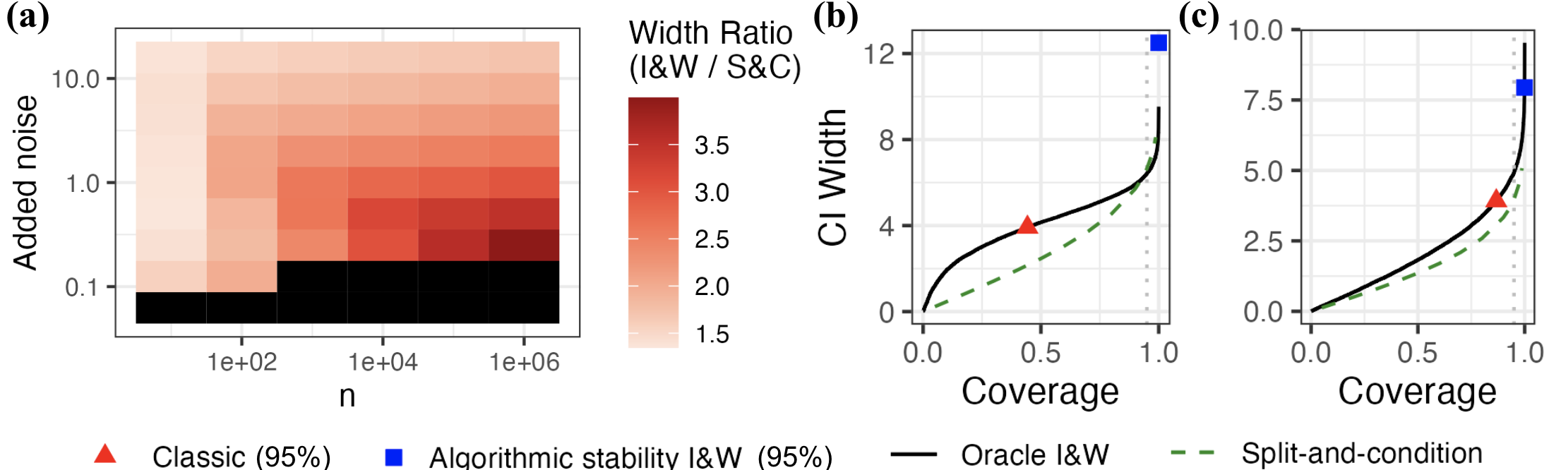
Thus, both (3.4) and (3.6) provide confidence intervals for that attain coverage . We should prefer the approach that yields narrower intervals. Figure 1(a) displays the ratio of the width of the infer-and-widen confidence interval (3.4) to the width of the split-and-condition confidence interval (3.6) when and , as we vary the sample size and the Laplacian variance in (3.3).
The infer-and-widen interval (3.4) involves tuning parameters and ; to construct Figure 1(a), for a fixed value of the noise and sample size in (3.3), we select the and that minimize the confidence interval width, subject to the constraints in Proposition 1. In the figure, black indicates values of and that necessitate a tiny quantile of the normal distribution, yielding numerical issues in R and therefore an interval (3.4) of apparently infinite width. The split-and-condition intervals are much narrower than the infer-and-widen intervals across all values of and considered.
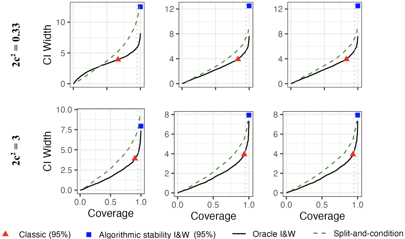
It is possible that the width of the infer-and-widen interval (3.4) is due to the fact that Zrnic and Jordan (2023) apply a series of inequalities in its derivation. Therefore, we now consider the “oracle” infer-and-widen interval: this is the narrowest possible interval centered at that achieves a given coverage. It is not computable in practice, as it requires knowledge of the true parameter value . In Figures 1(b, c), we numerically compare the “oracle” infer-and-widen method to the split-and-condition interval (3.6) under the selection rule (3.3) with variances and , respectively. In this setting, the “oracle” infer-and-widen interval is substantially wider than the split-and-condition interval in (3.6), thereby indicating that no infer-and-widen interval can outperform the split-and-condition interval (3.4) in this setting.
4 Vignette #2: Maximal contrasts
Following Zrnic and Jordan (2023), we consider the model 3.1 and suppose we also have access to a fixed design matrix with normalized columns . Our interest lies in the quantity defined via the selection rule
| (4.1) |
Zrnic and Jordan (2023) refer to this as the “maximal contrast”. If , then this setting is similar to Vignette #1, except with an absolute value in the selection rule.
To achieve a “stable” algorithm, Zrnic and Jordan (2023) consider the selection rule
| (4.2) |
where is a positive constant that governs the scale of additive noise.
Proposition 1 (An infer-and-widen interval based on (4.2), motivated by algorithmic stability (Zrnic and Jordan, 2023)).
We now construct a split-and-condition interval that makes use of the selection event (4.2). Note that is a function of . Since the distribution of is intractable, we cannot directly use it to derive a split-and-condition interval, as in Proposition 2. Proposition 2 instead makes use of the distribution of conditional on and some additional quantities.
Proposition 2 (A split-and-condition interval based on 4.2).
Consider the model in 3.1 and selection rule in 4.2. Define
where is defined in Subsection B.1. Let denote the CDF of the normal distribution with mean and variance , truncated to the set , and define and to satisfy
| (4.4) |
A split-and-condition confidence interval for takes the form
| (4.5) |
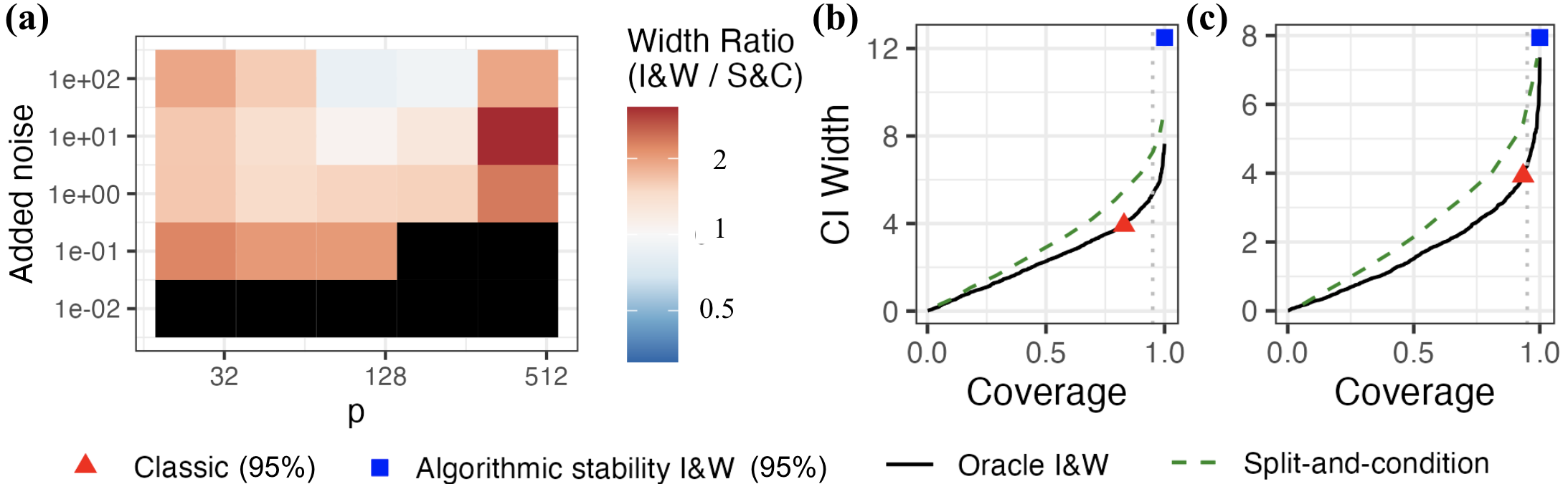
We now compare the interval (4.3) to (4.5), as well as to the “oracle” infer-and-widen interval using the Laplace selection rule (4.2). We simulate data according to 3.1 with and . We set where half of the elements of are zero and the other half are drawn from an exponential distribution with mean . The rows of are independent draws from with , and the columns of are scaled so that . Figure 2(a) displays the ratio of confidence interval widths across values of and the variance of the Laplacian noise in 4.2.
The infer-and-widen interval (4.5) involves tuning parameters and ; to construct Figure 2(a), for a fixed value of the noise and number of features in (4.2), we select the and that minimize the confidence interval width, subject to the constraints in Proposition 1. In the figure, black indicates values of and that necessitate a tiny quantile of the normal distribution, yielding numerical issues in R and therefore an interval (4.3) of apparently infinite width. The split-and-condition intervals are narrower than the infer-and-widen intervals across most values of and considered.
It is possible that the width of the infer-and-widen interval (4.3) is due to the fact that Zrnic and Jordan (2023) apply a series of inequalities in its derivation. Therefore, we now consider the “oracle” infer-and-widen interval: this is the narrowest possible interval centered at that achieves a given coverage. It is not computable in practice, as it requires knowledge of the true parameter value. In Figures 2(b, c), we numerically compare the “oracle” infer-and-widen method to the split-and-condition interval (4.5) under the selection rule (4.2) with variance and , respectively. In this setting, the “oracle” infer-and-widen interval is narrower than the split-and-condition interval in (4.5), thereby indicating that in principle, an infer-and-widen interval can outperform the split-and-condition interval (4.5) in this setting. However, to the best of our knowledge, no methods to construct such an infer-and-widen interval are currently available.
Remark 1.
Figure 2 of Zrnic and Jordan (2023) shows that the infer-and-widen interval (4.3) far outperforms a split-and-condition interval based on sample splitting in Vignette #2. In fact, in this setting, a split-and-condition interval based on sample splitting is pathological and better split-and-conditon intervals are available; see Subsection B.2. Thus, our results are not at odds with those of Zrnic and Jordan (2023).
5 Vignette #3: Inference after the lasso
We now consider inference on the set of coefficients selected by the lasso in a linear model (Tibshirani, 1996). We again consider the model 3.1, alongside a fixed design matrix with unit-normalized columns, i.e. . Our new selection rule is the magnitude-ordered set of features selected by the lasso:
| (5.1) | ||||
We then consider a least squares model fit to the features in . The target of inference is the coefficient of the feature with largest lasso magnitude, i.e. where
| (5.2) |
Here, the design matrix has columns ordered by the selected indices .
Zrnic and Jordan (2023) do not propose an infer-and-widen interval based on the lasso algorithm, as the lasso is not stable in the sense of Definition 1: while they do consider a variant of the lasso that is stable, it is far enough from the original lasso proposal that we do not investigate it here. Instead, we construct a split-and-condition interval based on Gaussian data thinning (Neufeld et al., 2024; Dharamshi et al., 2024), and then will consider the “oracle” infer-and-widen interval that makes use of the identical selection event.
Towards this end, we define
| (5.3) |
Proposition 1.
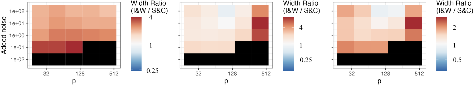
We compare the widths of the split-and-condition (5.4) and “oracle” infer-and-widen intervals — both of which have identical selection events — in Figure 3. We simulate data according to 3.1 with and . We set , where half of the elements of are zero and the other half are either zero or drawn from exponential distributions with means or in panels (a), (b), and (c) of Figure 3. The rows of are independent draws from with , and the columns of are scaled so that . Figure 3 displays the ratio of confidence interval widths as we vary and the variance of the Gaussian noise in (5.3).
We see from Figure 3 that the relative widths of the two intervals depend on details of the noise variance in (5.3) and distribution of . Of course, the “oracle” infer-and-widen interval cannot be computed in practice: any real-world infer-and-widen interval that achieves nominal coverage would necessarily be at least as wide as the oracle interval, if not far wider. Thus, while it may be possible to develop an infer-and-widen interval that might outperform the simple split-and-condition interval in 5.4 in specific scenarios, the potential upside of any such approach is extremely limited.
(a) (b) (c)
6 The bias of infer-and-widen intervals
We have seen in the previous sections that when infer-and-widen and split-and-condition intervals are formed for the same data-driven target of inference, the former tends to yield intervals that are far wider than the latter. We now investigate the reason for this. To facilitate the analysis, we consider Vignette #1 with a simple selection rule that uses Gaussian noise (as opposed to the Laplace noise used in (3.3)),
| (6.1) |
We know from Section 2.2 that any infer-and-widen interval is centered around .
Proposition 1 (Bounding the bias of the infer-and-widen midpoint).
That is, the bias increases on the order of . Note that as , i.e. the selection rule becomes fully random, this lower bound goes to zero as expected.
Noting that in (6.1) is independent of , it is straightforward to show that is a valid split-and-condition confidence interval for . Furthermore, , i.e. the midpoint of the split-and-condition interval is unbiased for the mean of the selected observation.
Thus, for finite , infer-and-widen here leads to a confidence interval that is centered in the wrong place, and the situation worsens as increases. By contrast, split-and-condition leads to a confidence interval that is correctly centered.
7 Discussion
Towards a better systematic understanding of the plethora of methods available for post-selection inference, in this paper we classified these methods into one of two frameworks: infer-and-widen and split-and-condition. We investigated the performance of these frameworks in three vignettes: two taken from Zrnic and Jordan (2023), and the third involving feature selection via the lasso. We constructed split-and-condition intervals that had exactly the same selection events as recently-proposed infer-and-widen intervals (Vignettes #1 and #2) or as an “oracle” infer-and-widen approach. Our findings are as follows:
-
1.
In the first two vignettes, when we devise split-and-condition and infer-and-widen intervals that have identical selection events, the former are substantially narrower than the latter.
-
2.
For a given nominal coverage, the “oracle” infer-and-widen interval is substantially narrower than the interval arising from algorithmic stability, which is the current state-of-the-art approach for the infer-and-widen framework (Zrnic and Jordan, 2023). Stated another way, while algorithmic stability may be the best infer-and-widen method to date, there is still room for improvement in constructing tighter intervals.
-
3.
Nonetheless, we can in some cases obtain a simple and easy-to-compute split-and-condition interval that outperforms the “oracle” infer-and-widen approach (in the sense of having a narrower interval width for a given selection error). Thus, the benefit of developing improved infer-and-widen methods is limited or non-existent.
Why does split-and-condition so often outperform infer-and-widen? The answer is simple: the latter yields intervals centered around a biased estimator of the target of inference, whereas the former faces no such restriction. This point was illustrated in Section 6.
We close with two remarks, firstly about the case of a deterministic selection rule. Zrnic and Jordan (2023) point out that because such a rule is -stable in the sense of Definition 1, the algorithmic stability interval is simply the classical interval (see Theorem 2). Of course, the same is true for split-and-condition: in the case of a deterministic selection rule, we can take and , using the notation in Section 2; then, the split-and-condition interval is simply the classical interval.
Secondly, it is worth mentioning the results of Goeman and Solari (2022), who proved that any split-and-condition method is dominated by an unconditional multiple testing procedure defined on the full universe of hypotheses. In contrast, we examine unconditional methods which (1) are defined only on the selected hypotheses and (2) are in the infer-and-widen framework. For instance, a Bonferroni correction provides valid inference on the selected mean in Vignette #1, but is dominated in power by Bonferroni-corrected tests of all possible means. Our comparisons reflects a study of existing approaches and practices.
Acknowledgements
We acknowledge funding from the following sources: ONR N00014-23-1-2589, NSF DMS 2322920, a Simons Investigator Award in Mathematical Modeling of Living Systems, and NIH 5P30DA048736.
References
- Andrews et al. [2019] Isaiah Andrews, Toru Kitagawa, and Adam McCloskey. Inference on winners. Working Paper 25456, National Bureau of Economic Research, January 2019.
- Berk et al. [2013] Richard Berk, Lawrence Brown, Andreas Buja, Kai Zhang, and Linda Zhao. Valid post-selection inference. The Annals of Statistics, 41(2):802–837, April 2013. ISSN 0090-5364, 2168-8966. Publisher: Institute of Mathematical Statistics.
- Bonferroni [1936] C. Bonferroni. Teoria statistica delle classi e calcolo delle probabilita. Pubblicazioni del R Istituto Superiore di Scienze Economiche e Commericiali di Firenze, 8:3–62, 1936.
- Chen and Bien [2020] Shuxiao Chen and Jacob Bien. Valid inference corrected for outlier removal. Journal of Computational and Graphical Statistics, 29(2):323–334, 2020.
- Chen and Witten [2023] Yiqun T. Chen and Daniela M. Witten. Selective inference for k-means clustering. Journal of Machine Learning Research, 24(152):1–41, 2023. ISSN 1533-7928.
- Cox [1975] D. R. Cox. A note on data-splitting for the evaluation of significance levels. Biometrika, 62(2):441–444, August 1975. ISSN 0006-3444.
- Dharamshi et al. [2024] Ameer Dharamshi, Anna Neufeld, Keshav Motwani, Lucy L. Gao, Daniela Witten, and Jacob Bien. Generalized data thinning using sufficient statistics. Journal of the American Statistical Association, 0(0):1–13, 2024.
- Dwork and Roth [2014] Cynthia Dwork and Aaron Roth. The algorithmic foundations of differential privacy. Found. Trends Theor. Comput. Sci., 9(3–4):211–407, aug 2014. ISSN 1551-305X.
- Fithian et al. [2017] William Fithian, Dennis Sun, and Jonathan Taylor. Optimal Inference After Model Selection, April 2017. arXiv:1410.2597.
- Gao et al. [2024] Lucy L. Gao, Jacob Bien, and Daniela Witten. Selective Inference for Hierarchical Clustering. Journal of the American Statistical Association, 119:332–342, October 2024.
- Goeman and Solari [2022] Jelle Goeman and Aldo Solari. Conditional Versus Unconditional Approaches to Selective Inference, July 2022. arXiv:2207.13480 [stat].
- Holm [1979] Sture Holm. A Simple Sequentially Rejective Multiple Test Procedure. Scandinavian Journal of Statistics, 6(2):65–70, 1979. Publisher: [Board of the Foundation of the Scandinavian Journal of Statistics, Wiley].
- Hyun et al. [2018] Sangwon Hyun, Max Grazier G’Sell, and Ryan J. Tibshirani. Exact post-selection inference for the generalized lasso path. Electronic Journal of Statistics, 12:1053–1097, 2018.
- Hyun et al. [2021] Sangwon Hyun, Kevin Z. Lin, Max G’Sell, and Ryan J. Tibshirani. Post-selection inference for changepoint detection algorithms with application to copy number variation data. Biometrics, 77(3):1037–1049, September 2021.
- Jewell et al. [2022] Sean Jewell, Paul Fearnhead, and Daniela Witten. Testing for a Change in Mean after Changepoint Detection. Journal of the Royal Statistical Society Series B: Statistical Methodology, 84(4):1082–1104, September 2022.
- Kamath [2015] Gautam Kamath. Bounds on the expectation of the maximum of samples from a gaussian. Technical report, University of Waterloo, 2015.
- Lee et al. [2016] Jason D. Lee, Dennis L. Sun, Yuekai Sun, and Jonathan E. Taylor. Exact post-selection inference, with application to the lasso. The Annals of Statistics, 44(3):907 – 927, 2016.
- Leiner et al. [2023] James Leiner, Boyan Duan, Larry Wasserman, and Aaditya Ramdas. Data fission: Splitting a single data point. Journal of the American Statistical Association, 0(0):1–12, 2023.
- Neufeld et al. [2024] Anna Neufeld, Ameer Dharamshi, Lucy L. Gao, and Daniela Witten. Data Thinning for Convolution-Closed Distributions. Journal of Machine Learning Research, 25(57):1–35, 2024.
- Neufeld et al. [2022] Anna C. Neufeld, Lucy L. Gao, and Daniela M. Witten. Tree-Values: Selective Inference for Regression Trees. Journal of Machine Learning Research, 23(305):1–43, 2022.
- Panigrahi et al. [2024] Snigdha Panigrahi, Kevin Fry, and Jonathan Taylor. Exact selective inference with randomization. Biometrika, April 2024. ISSN 1464-3510.
- Rasines and Young [2023] D García Rasines and G A Young. Splitting strategies for post-selection inference. Biometrika, 110(3):597–614, September 2023. ISSN 1464-3510.
- Scheffé [1959] Henry Scheffé. The analysis of variance. Wiley, Oxford, England, 1959.
- Tian and Taylor [2018] Xiaoying Tian and Jonathan Taylor. Selective Inference with a Randomized Response. The Annals of Statistics, 46(2):679–710, 2018. ISSN 0090-5364. Publisher: Institute of Mathematical Statistics.
- Tibshirani [1996] Robert Tibshirani. Regression shrinkage and selection via the lasso. Journal of the Royal Statistical Society Series B: Statistical Methodology, 58(1):267–288, 1996.
- Zrnic and Jordan [2023] Tijana Zrnic and Michael I. Jordan. Post-selection inference via algorithmic stability. The Annals of Statistics, 51(4):1666–1691, August 2023. ISSN 0090-5364, 2168-8966. Publisher: Institute of Mathematical Statistics.
- Šidák [1967] Zbyněk Šidák. Rectangular Confidence Regions for the Means of Multivariate Normal Distributions. Journal of the American Statistical Association, 62(318):626–633, June 1967. ISSN 0162-1459.
Appendix A Vignette #1
A.1 Proof of Proposition 2
To construct a split-and-condition confidence interval under the selection rule 3.2, it suffices to characterize the distribution , where and . This conditional distribution is difficult to characterize, however, and so we instead consider the distribution conditional on and an additional event.
Lemma 1 (Data fission with Laplace noise).
Let where . Let where . Define , , and the set . Then the density of the conditional distribution has the following form:
| (A.1) |
where denotes an -dimensional multivariate normal distribution truncated to the set .
Proof.
The conditional density is as follows:
| (A.2) |
Thus the density of is that of multivariate normal distribution with independent marginals, truncated to , which restricts the domain to the intersection of halfspaces defined by elements of . ∎
It remains to derive a confidence interval for . Note that since is a truncated normal distribution with a diagonal covariance, the marginal distributions are also truncated normal distributions (note that this is not in general true for an arbitrary covariance). Thus the marginal distribution , where A valid post-selection confidence interval for follows from the CDF of this truncated normal distribution, yielding Proposition 2.
A.2 Proof of Proposition 1
First, since ,
To bound the conditional expectation, let , where is the additive noise. Thus, . Let , with maximum order statistic . We can bound the conditional expectation
where the final inequality comes from Kamath [2015]. Taking the expectation on each side completes the proof.
Appendix B Vignette #2
B.1 Proof of Proposition 2
Proof.
The proof will make use of Theorem 5.2 of Lee et al. [2016], which we restate now.
Theorem 1 (Theorem 5.2 of Lee et al. [2016]).
Let an -dimensional random vector, and a vector of interest. For any fixed matrix and vector , define
and the pair
Then
| (B.1) |
where denotes a normal distribution truncated to .
Returning to our setting under the model in 3.1 with a fixed and column-normalized design matrix , for brevity let and where . Recall that our target of inference is , where is the selection rule in 4.2. This selection rule is implicitly a function of the Laplacian noise , and so to emphasize this point we will write in this section.
To construct a confidence interval, as in 2.6 it will suffice to derive the distribution of where , e.g. we will condition on the selection event along with an additional event. By the law of total probability, conditional coverage implies marginal coverage.
We will show that there exists a matrix for which
| (B.2) |
where
| (B.3) |
Henceforth, for brevity, we will denote by .
To show that there exists a matrix for which (B.2) holds, note that by definition, if and only if for all . In turn, expanding the absolute value and definition of , (B.2) holds if and only if both (I) and (II) hold:
-
(I)
if , then for all it holds that
-
(a)
,
-
(b)
,
-
(c)
;
-
(a)
-
(II)
else if , then for all it holds that
-
(a)
,
-
(b)
,
-
(c)
.
-
(a)
We further rearrange the above inequalities to collect the terms on one side, as follows:
-
(I)
If , then for all it holds that
-
(a)
,
-
(b)
,
-
(c)
;
-
(a)
-
(II)
else if , then for all it holds that
-
(a)
,
-
(b)
,
-
(c)
.
-
(a)
Thus, if , then we are in case (I), and if and only if satisfies , where
| (B.4) |
and we denote and for brevity. If instead , then we are in case (II), where if and only if satisfies . Thus, in either case, if and only if , and so, by definition of , if and only if . This establishes that (B.2) holds for defined in (B.4).
Thus, by B.2, we see that
We would like to apply Theorem 1 to the right-hand side of this result with and , but these are random quantities and so we will need to fix them by conditioning on and .
Defining as in Theorem 1, we have that
| (B.5) | |||
| (B.6) | |||
| (B.7) | |||
| (B.8) |
To establish B.7, note that the event is composed of a system of inequalities, the first of which states that , or equivalently, that . Recalling the definition of in (B.3), it follows that the event implies that . This yields (B.7).
Finally, recall that . Note that , , and the event are functions of , and thus all three are independent of . B.8 follows.
We now apply Theorem 1 with , , , and . Furthermore, recalling that is column-normalized, we have that and in the statement of Theorem 1. Thus,
| (B.9) |
for and given in the statement of Proposition 2, which are functions of and through and .
A confidence interval for is thus obtained using the CDF of the above truncated normal distribution. This in turn provides valid unconditional coverage for by the law of total probability. ∎
B.2 Sample splitting versus data thinning
Not all split-and-condition methods are alike. For instance, at first glance, it may appear that sample splitting and data thinning [Rasines and Young, 2023, Neufeld et al., 2024, Dharamshi et al., 2024] are comparable: both approaches yield independent training and test sets, and the widths of their confidence intervals depend on the fraction of the Fisher information in the test set. However, the two methods can fundamentally differ wildly. This explains why our results for Vignette #2 in Section 4 comparing algorithmic stability to split-and-condition approaches other than sample splitting, with identical selection events, differ from the results seen in Figure 2 of Zrnic and Jordan [2023].
Consider the setup in Section 4 with , and let and . Suppose we conduct sample splitting and put fraction of the observations into the training sets , and the rest into the test sets . Let . Then, since with probability the training set contains the row of corresponding to the maximal magnitude element of . Note that this probability is independent of . Furthermore, the th column in is necessarily a column of zeros, since is the identity and the th column of had a one in it. Thus, is a degenerate distribution with mean and variance .
In contrast, data thinning constructs independent folds and , . Let . Then, occurs with probability dependent on , , and . Furthermore, , leading to a non-degenerate distribution. We see that both selection and inference differ substantially from sample splitting in this case.
B.3 Additional simulation results
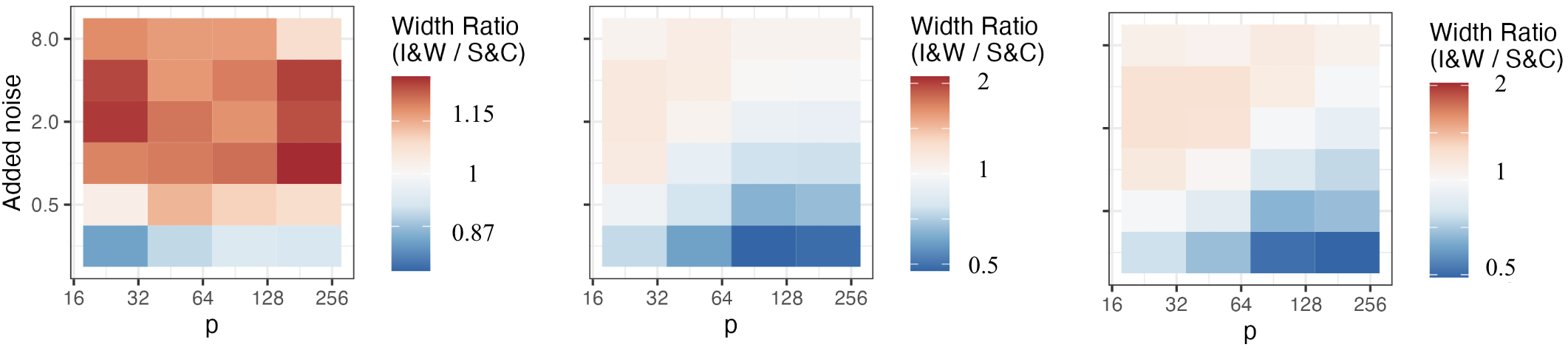
The simulation results in Section 4 reflect a limited set of parameter choices. Figure 4 extends Figure 2(a) to a wider range of levels of signal. Figure 5 extends Figures 2(b, c) to a wider range of levels of signal.
(a) (b) (c)
Appendix C Vignette #3
C.1 Proof of LABEL:{thm:vignette-3-gaussian-DT}
The result follows from independence of the selection and inference stages, per the following result.
Lemma 1 (Gaussian data thinning, Rasines and Young [2023], Neufeld et al. [2024]).
Assume , where is unknown and is known. For any , let , and define and . Then , , and .
Thus the selection event in 5.1, a function of through , is independent of . Hence, inference conducted on is independent of the selection event and hence is valid. We proceed to conduct conventional inference in an ordinary least squares model on the first selected coefficient, using the known variance , as given in Section 4.1 of Berk et al. [2013].