EqNIO: Subequivariant Neural Inertial Odometry

Abstract

Neural networks are seeing rapid adoption in purely inertial odometry, where accelerometer and gyroscope measurements from commodity inertial measurement units (IMU) are used to regress displacements and associated uncertainties. They can learn informative displacement priors, which can be directly fused with the raw data with off-the-shelf non-linear filters. Nevertheless, these networks do not consider the physical roto-reflective symmetries inherent in IMU data, leading to the need to memorize the same priors for every possible motion direction, which hinders generalization. In this work, we characterize these symmetries and show that the IMU data and the resulting displacement and covariance transform equivariantly, when rotated around the gravity vector and reflected with respect to arbitrary planes parallel to gravity. We design a neural network that respects these symmetries by design through equivariant processing in three steps: First, it estimates an equivariant gravity-aligned frame from equivariant vectors and invariant scalars derived from IMU data, leveraging expressive linear and non-linear layers tailored to commute with the underlying symmetry transformation. We then map the IMU data into this frame, thereby achieving an invariant canonicalization that can be directly used with off-the-shelf inertial odometry networks. Finally, we map these network outputs back into the original frame, thereby obtaining equivariant covariances and displacements. We demonstrate the generality of our framework by applying it to the filter-based approach based on TLIO, and the end-to-end RONIN architecture, and show better performance on the TLIO, Aria, RIDI and OxIOD datasets than existing methods.

1 Introduction

Inertial Measurement Units (IMUs) are critical sensors that measure the forces and angular velocities experienced by a body. These sensors are essential for applications such as robot navigation and AR/VR, where they facilitate precise and rapid tracking of inertial frames. Visual Inertial Odometry (VIO) approaches that combine an IMU and camera sensors have achieved impressive performance in accurately estimating camera poses. However, VIO methods are prone to failure when the image sensor fails in challenging lighting conditions. Recently, a class of novel methods has attempted to push the limit of IMU-only odometry by training a "statistical" IMU represented as a neural network [33, 30]. These approaches perform competitively against VIO methods using only a single IMU sensor. Despite these impressive results, these approaches rely heavily on motion patterns learned from the training data. In particular, the networks trained on a particular configuration of the IMU do not easily generalize to a different test setting due to the rotation of the body frames. This is particularly relevant if we want to do more than just forward-moving motions and allow flexible mounting of the IMU sensors. This issue is illustrated in Figure 1, where the rotated inputs fail to yield appropriately rotated trajectories with TLIO [33] due to the network’s inability to ensure equivariance. In contrast, EqNIO ensures rotation and reflection equivariance ($O(2)$), enabling it to handle rotations and reflections unseen during training.

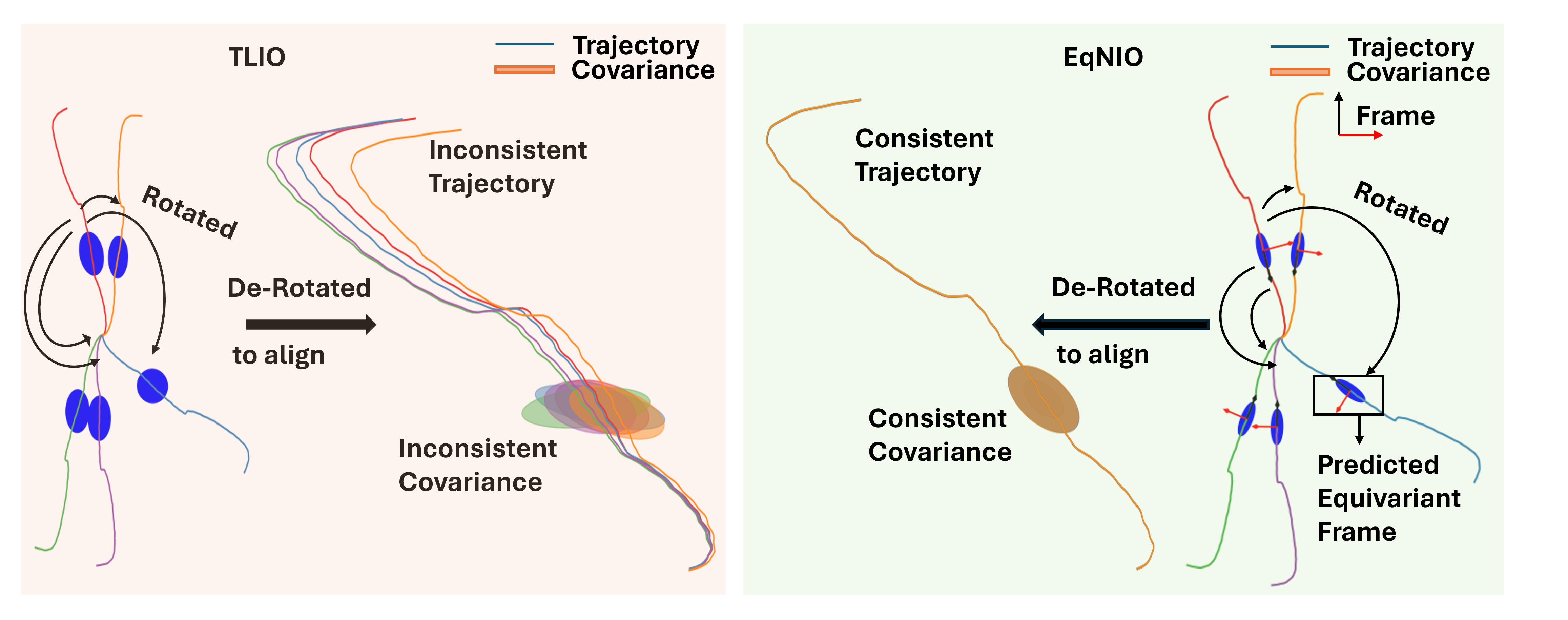
Figure 1: Left: the predicted trajectories and covariance ellipsoids from the non-equivariant TLIO baseline are displayed for 5 identical trajectories with different IMU frames during inference. The de-rotated trajectories and ellipsoids demonstrate significant inconsistency. Right: we show that the de-rotated trajectories and covariances from the equivariance-enabled EqNIO are perfectly aligned.

We hypothesize that this lack of robustness stems from the network’s failure to leverage the inherent geometric symmetry in the environment, which compels the network to overfit to the motion patterns relative to the training data frames. Although strategies like rotational augmentations have been suggested to mitigate these challenges, they significantly increase the training complexity and computational demands. Moreover, achieving approximate equivariance through training data augmentation does not ensure consistent outputs under transformations, as shown in Figure 1.

In this study, we address the symmetry problem in IMU measurements, influenced by gravity and the vital role of gyro data, by modeling it as a problem of subequivariance. This is further aligned with $SO(2)$ and $O(2)$ equivariance. We introduce a novel framework to predict a subequivariant frame, tailored to canonicalize sequential IMU data, enabling subequivariant predictions of both displacement and covariance. Specifically, the network designed to predict the frame is inherently subequivariant, incorporating subequivariant basic layers intentionally crafted. The frame predicted is aligned with the principal axes of the covariance matrix, as shown in Figure 1, enhancing the efficient learning of subequivariant covariance. We demonstrate that our subequivariant networks can be seamlessly integrated with existing methods such as TLIO and RONIN, enhancing end-to-end odometry performance. Our approach is thoroughly validated through experimental trials on multiple real-world datasets. Here is a summary of our contributions: (i) Modeling subequivariance: We derive the inherent symmetry of IMU data as subequivariance, which is refined to $SO(2)$ or $O(2)$ equivariance through designed preprocessing. (ii) Subequivariant Framework: We introduce a novel subequivariant framework specifically designed for inertial-only odometry, enhancing robustness and generalizability across different motion patterns and sensor configurations. We present the theoretical backbone for applying the framework to an odometry network under $O(2)$ and $SO(2)$ transformations. (iii) Comprehensive Evaluation and State-of-the-Art Performance: We perform a detailed quantitative analysis to compare our subequivariant neural networks with several baseline methods across diverse datasets. This evaluation confirms the superiority of our approach. Our method establishes a new standard for state-of-the-art performance in inertial-only odometry, significantly enhancing accuracy and reliability compared to existing techniques.

2 Related Work

2.1 Inertial Odometry

Purely Inertial Odometry can be broadly classified into two categories: kinematics-based approaches and learning-based approaches. The kinematics-based approaches [42, 3] leverage analytical solutions based on double integration that suffer from drift accumulation over time when applied to consumer-grade IMUs. A kinematics-based approach that requires loop closures has been explored by Solin et al. [38]. Other approaches [27, 29, 4] rely on crafting pseudo measurements for an Extended Kalman Filter where only IMU measurements are the source of information. This has been extensively studied in Pedestrian Dead Reckoning [32] where a variety of models have been developed for step counting [31, 4], detecting when the system is static [26, 35] and gait estimation [2] to mention a few.

Learning-based approaches using CNNs, RNNs, LSTMs, and TCN have been used to regress velocity, which alleviates the curse of inertial tracking. RIDI [52] and PDRNet [1] use a hierarchical approach with a subgroup classification module to identify the location and build separate type-specific regression modules. RIDI uses the regressed velocity to correct the IMU measurements, while RONIN [30] directly integrates the regressed velocities but assumes orientation information. Denoising networks have been used to either regress the biases [6, 7, 5] or output the denoised IMU measurements [39]. Buchanan et al. [7] build a device-specific IMU noise modeling architecture and use constant covariance while AI-IMU [5] estimates the covariance for automotive applications. Displacement-based neural network methods like IONet [10], TLIO [33], RNIN-VIO [13], and IDOL [40] directly estimate 2D/3D displacement. IONet uses LSTM to reduce integration drift, while TLIO employs Resnet18, regressing both displacement and uncertainty to update an Extended Kalman Filter for estimating the full 6DOF pose and IMU biases. Unlike TLIO, which only regresses the diagonal of the covariance matrix, Russell and Reale [36] parametrizes the full covariance matrix using Pearson correlation. RNIN-VIO extends TLIO’s methods to account for continuous human motion and regresses displacement in a global frame, adding a loss function for long-term accuracy. IDOL separately estimates orientation.

Equivariant Inertial Odometry

The previous learning-based approaches [33, 13] use random $SO(2)$ augmentation strategies to achieve approximate $SO(2)$ equivariance. MotionTransformer [12] used GAN-based RNN encoder approach to transfer IMU data into domain-invariant space by separating the domain-related constant. Recently, RIO [8] demonstrated the benefits of rotational equivariance with an auxiliary loss and introduced Adaptive Test Time Training (TTT) and a deep ensemble of models for uncertainty estimation despite TTT’s increased computation and inference time. We propose integrating equivariance directly into the framework for guaranteed rotational consistency. Additionally, no prior work has addressed reflection equivariance, which is not straightforward since gyroscope data adhere to the right-hand rule. Our novel $O(2)$ equivariant framework easily adapts to existing learning-based inertial navigation systems, showing benefits on TLIO and RONIN.

2.2 Equivariant Networks

Group equivariant networks [16] provide deep learning pipelines that are equivariant by design with respect to group transformations of the input. Extensive research has been conducted on how these networks process a variety of inputs, including point clouds [41, 14, 20], 2D [49, 46], 3D [47, 22], and spherical images [18, 21, 23, 24], graphs [37] and general manifolds [19, 17, 48, 51]. However, for a sequence of vectors and scalars, there is no current applicable equivariant model for the prediction of motion prior with IMU data, and we are the first to apply the equivariant model for neural integration of IMUs. On the other hand, general theories and methods have been developed for networks that are equivariant to $E(n)$ and its subgroups. Cesa et al. [9], Xu et al. [50] utilize Fourier analysis to design the steerable kernels in CNNs on homogeneous space, while Finzi et al. [25] proposed a numerical algorithm to compute a kernel by solving the linear equivariant map constraint. Additionally, [44] demonstrated that any $O(n)$ equivariant function can be represented using a set of scalars and vectors. However, applying these general approaches to the IMU prediction problem is not straightforward. Gravity’s presence introduces subequivariance, the angular velocity in the input data follows the right-hand rule, and the input is a sequence with a time dimension. These factors make the direct application of the vast theory available on equivariant networks challenging. Related works [28, 15] tackle subequivariance using equivariant graph networks and calculating gram matrices for invariant weights for vectors and gravity, achieving simple $O(2)$ equivariance when data doesn’t obey the right-hand rule. Our approach handles data sequences and employs specially designed linear layers, nonlinearities, and normalization for $SO(2)$ and $O(2)$, respectively, seamlessly integrating them into architectures like CNNs and transformers. Additionally, we tackle the reflection equivariance challenge posed by the right-hand rule through a bijection map aligning data with $O(2)$ equivariant spaces.

3 Problem Setup

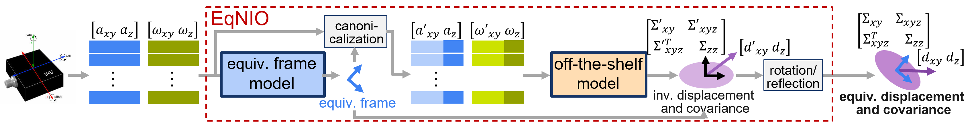
(a)

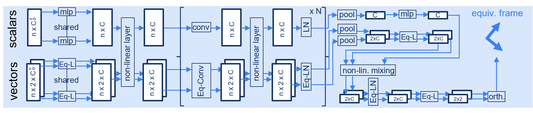
(b)

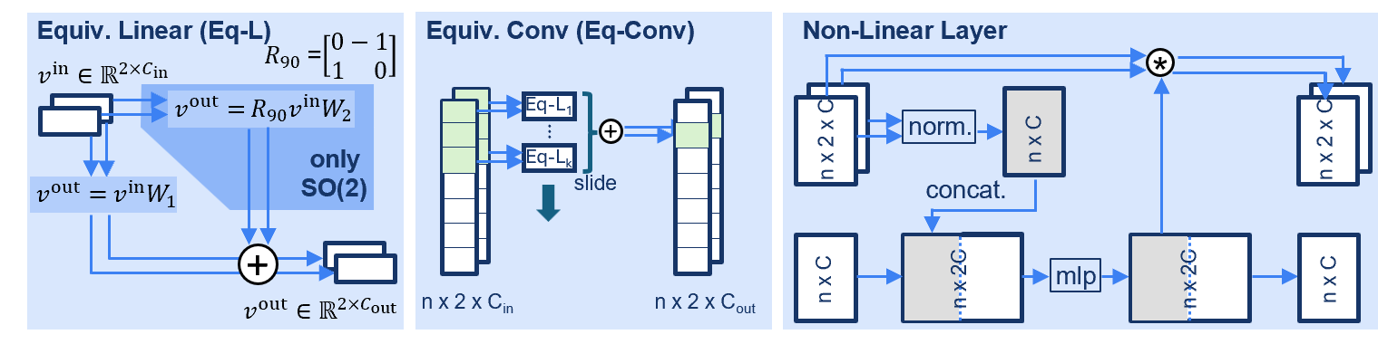
(c)

Figure 2: EqNIO (a) processes sequences of gravity-aligned IMU measurements, $\{(a_{i},\omega_{i})\}_{i=1}^{n}$. An equivariant network (blue) predicts a canonical equivariant frame on the plane orthogonal to gravity. The input sequence is then mapped into this frame, i.e. canonicalized, to obtain invariant inputs $\{(a^{\prime}_{i},\omega^{\prime}_{i})\}_{i=1}^{n}$. An off-the-shelf model (conventional neural network) uses them to predict invariant displacement ($d^{\prime}$) and covariance ($\Sigma^{\prime}$) which are later mapped back into the original frame to obtain equivariant displacement ($d$) and covariance ($\Sigma$). The equivariant network architecture (b) preprocesses the inputs to $n\times C_{0}^{s}$ scalars, and $n\times C_{0}^{v}$ vectors: Vectors are processed by equivariant linear layers (Eq-L), convolutional layers (Eq-Conv), and normalization layers (Eq-LN), while scalars are separately processed with conventional layers. The vector and scalar features interact only in the non-linear layer in an equivariant way. Eq-L (c, left) uses two weights $W_{1},W_{2}$ for SO(2) equivariance, and only $W_{1}$ for O(2) equivariance. Eq-L (c, middle) uses Eq-L to perform 1-D convolutions over time. The equivariant non-linear layer (c, right) mixes the vector and scalar features.

This paper aims to estimate the orientation, position, and/or velocity of a rigid body over time given a sequence of IMU accelerometer (giving accelerations $a_{i}\in\mathbb{R}^{3}$) and gyroscope (giving angular velocity $\omega_{i}\in\mathbb{R}^{3}$) measurements $\{(a_{i},\omega_{i})\}_{i=1}^{n}$, expressed in the local IMU inertial frame. Simply integrating these measurements results in large drift due to sensor noise and biased IMU readings, and thus, we use off-the-shelf neural networks to regress accurate 3 degrees-of-freedom (DoF) linear velocities [30] or 3D displacement measurements $d\in\mathbb{R}^{3}$ and covariances $\Sigma\in\mathbb{R}^{3\times 3}$ [33]. In the latter case, we treat the network outputs as measurements and fuse them in an Extended Kalman Filter (EKF) estimating the IMU state, i.e. orientation, position, velocity, IMU biases, and uncertainties. Preliminaries on the terms used in inertial odometry are included in Appendix A.1.2. Preliminaries and details on EKFs and the associated IMU measurement model are included in Appendix A.4.

To reduce the data variability in IMU measurements, we map them to a gravity-aligned frame (i.e. perform gravity-alignment), which has its z-axis aligned with the gravity direction. We do this by simple rotations. Typically, the gravity direction can be estimated from an auxiliary visual-inertial odometry (VIO) method or can be estimated from the dominant direction of accelerometer readings at rest during training. During test time, the orientation estimated from the current state of the EKF or known orientation is used for gravity-alignment. Reducing the data variability aids in learning priors associated with particular IMU motions, and also simplifies odometry due to the elimination of two degrees of freedom. This frame is, however, ill-defined, since simply rotating it around z or reflecting it across planes parallel to z (applications of rotations or roto-reflections from the groups $SO(2)$ and $O(2)$) result in new valid gravity-aligned frames. Our main contribution is to eliminate these additional degrees of variability in IMU data with an $\bm{SO(2)}$ or $\bm{O(2)}$ equivariance framework, and thus facilitate more efficient learning of motion priors.

Our framework operates in three steps as seen in Figure 2(a): After gravity alignment, it first estimates a canonical frame using an equivariant neural network. Then, it maps the IMU data into this frame, i.e. canonicalizes them, before predicting linear velocity or displacement and covariance with an off-the-shelf neural network $\Phi$. Finally, it uses the canonical frame to map the resulting quantities into the original frame. In the language of equivariance research, our method thus has the property that transforming the gravity-aligned frame with the aforementioned symmetries (and as a result, the IMU data expressed in that frame) leads to an equivariant change in the resulting displacement and covariances. Unlike related approaches [30, 33, 8], which enforce this property with yaw augmentations or auxiliary losses (i.e. possess non-strict equivariance), our method enforces this property exactly (strict $O_{\vec{g}}(3)$ equivariance), and by design.

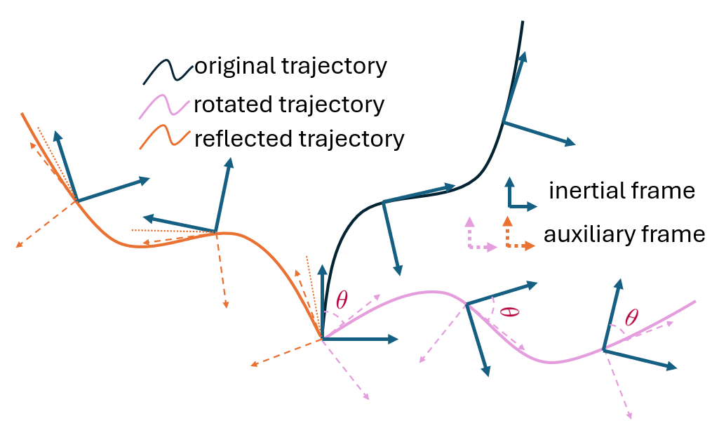
Figure 3: In this 2D case, the inertial and local gravity-aligned frames are aligned, showing an original (blue), rotated (purple), and reflected trajectory (orange). The inertial frame (blue) changes along each trajectory. Along the rotated and reflected trajectories, auxiliary frames are introduced where accelerations and rotations represented are the same as those represented in the inertial frame of the original trajectory. Consequently, both inputs (acceleration and rotation) and displacements are rotated or reflected accordingly in the inertial frames along these two trajectories.

Similar to prior works [15, 28], the presence of gravity breaks symmetry in the z-axis which is aligned with the gravity $\vec{g}\in\mathbb{R}^{3}$. Hence, the orthogonal symmetry $O(3)$ is no longer preserved in all directions. In fact, it is only preserved for the subgroup $O_{\vec{g}}(3):=\{R\in O(3)|R\vec{g}=\vec{g}\}$ where $R\in O(3):=\{R\in\mathbb{R}^{3\times 3}|R^{T}R=I\}$. This relaxation of strict $O(3)$ equivariance in the gravity direction is termed as $O_{\vec{g}}(3)$ equivariance or $O(3)$ subequivariance. Similarly, the subgroup $SO_{\vec{g}}(3):=\{R\in SO(3)|R\vec{g}=\vec{g}\}$ where $R\in SO(3):=\{R\in\mathbb{R}^{3\times 3}|R^{T}R=I,\text{det}(R)=1\}$. Denote $R_{3\times 3}\in\mathbb{R}^{3\times 3}\subset O_{\vec{g}}(3)$ an orthonormal roto-reflection operator which rotates vectors around the $z$-axis (axis aligned with gravity direction), and reflects them along a plane parallel to the $z$-axis if $\text{det}(R_{3\times 3})=-1$. Figure 3 illustrates the effect of $R_{3\times 3}$ on displacements and the resulting trajectory. Since $R_{3\times 3}$ only affects the $xy$ components of vectors $v$ and keeps their $z$ components, we decompose $R_{3\times 3}=R_{2\times 2}\oplus 1$ (where $\oplus$ composes $R_{2\times 2}$ and $1$ in block diagonal form), and $v=(v_{xy},v_{z})$ into their separate components. Since $R_{3\times 3}$ is fully defined by $R_{2\times 2}$, we can directly identify it with the rotation matrix $R_{2\times 2}$ which is part of the smaller subgroup $SO(2):=\{R\in\mathbb{R}^{2\times 2}|R^{T}R=I,\text{det}(R)=1\}$ or $O(2):=\{R\in\mathbb{R}^{2\times 2}|R^{T}R=I\}$. In fact, the above argument implies that $SO(2)$ and $SO_{\vec{g}}(3)$ are isomorphic, i.e. $SO(2)\cong SO_{\vec{g}}(3)$ (and similarly $O_{\vec{g}}(3)\cong O(2)$) and so for the remainder of the paper we will simply use the terms $SO(2)$ and $O(2)$ equivariance. Moreover, we refer to the xy-components $v_{xz}$ of vectors that transform with $R_{2\times 2}$ as equivariant vectors and the z-components $v_{z}$ that remain unchanged by $R_{2\times 2}$ as invariant scalars. We formalize and achieve equivariance with the tools of group and representation theory, and include necessary preliminaries in the Appendix A.1.1. We train an off-the-shelf neural network $\Phi:\mathbb{R}^{n\times 2\times 3}\rightarrow\mathbb{R}^{3}\times\ \mathbb{R}^{3\times 3}$ that takes as input a sequence of $n$ IMU measurements $\{(a_{i},\omega_{i})\}_{i=1}^{n}$ in a gravity-aligned frame and regresses 3D displacement ($d\in\mathbb{R}^{3}$) and covariance ($\Sigma\in\mathbb{R}^{3\times 3}$) in the same frame, and thus

$$d,\Sigma=\Phi(\{(a_{i},\omega_{i})\}_{i=1}^{n})$$ (1)

We design separate networks that handle $SO(2)$ and $O(2)$ equivariance, i.e. have the property $\Phi(\{(\rho_{a}(R_{2\times 2})a_{i},\rho_{\omega}(R_{2\times 2})\omega_{i})\}_{i=1}^{n})=\rho_{o}(R_{2\times 2})\Phi(\{(a_{i},\omega_{i})\}_{i=1}^{n})$. Here $\rho$ denotes a group representation and generates suitable transformation matrices for acceleration $(\rho_{a})$, angular velocity $(\rho_{\omega})$, and output variables $\rho_{o}$ under the action of $R_{2\times 2}$. The representation $\rho_{o}$ in particular decomposes into $\rho_{o}=\rho_{d}\oplus\rho_{\Sigma}$, where $\rho_{d}$ and $\rho_{\Sigma}$ act separately on the displacement and covariance generated by the neural network. For accelerations and displacements, $\rho_{a}(R_{2\times 2})=R_{2\times 2}\oplus 1$ and $\rho_{d}(R_{2\times 2})=R_{2\times 2}\oplus 1$, while for angular velocities $\rho_{\omega}(R_{2\times 2})=\text{det}(R_{2\times 2})(R_{2\times 2}\oplus 1)$. Upon reflection, the rotation direction of $\omega$ must be additionally inverted, which is why we add a factor of $\text{det}(R)$, and is further illustrated in Figure 4(a). When designing the equivariant network, we desire all input quantities to transform similarly. For this reason, when dealing with $O_{\vec{g}}(3)$ equivariance, we will later introduce an additional preprocessing step, which decomposes $\omega=v_{1}\times v_{2}$. These vectors transform in the same way as acceleration, i.e. $\rho_{v_{2}}(R_{2\times 2})=\rho_{v_{1}}(R_{2\times 2})=R_{2\times 2}\oplus 1$, and lead to the desired transform of resulting $\omega$. Finally, covariance $\Sigma$ transforms as $(R_{2\times 2}\oplus 1)\Sigma(R_{2\times 2}\oplus 1)^{T}$. If we write $\Sigma$ in vectorized form we have $\text{vec}(\Sigma)^{\prime}=(R_{2\times 2}\oplus 1)\otimes(R_{2\times 2}\oplus 1)\text{vec}(\Sigma)$ so $\rho_{\Sigma}(R_{2\times 2})=(R_{2\times 2}\oplus 1)\otimes(R_{2\times 2}\oplus 1)$. Here $\otimes$ denotes the Kronecker product between matrices.

4 Subequivariant Framework

4.1 Preprocessing

As mentioned in Section 3, accelerations and angular velocities do not transform the same way under an action of $R_{2\times 2}\in O(2)$ when there is a reflection involved. To address this, we decompose the angular rate into vectors $v_{1},v_{2}$ such that $\omega=v_{1}\times v_{2}$ (see Figure 4(b)). Both vectors transform as $v^{\prime}_{1/2}=(R_{2\times 2}\oplus 1)v_{1/2}$ under rotation $R_{2\times 2}$, identical to the acceleration, and their cross product has the desirable property $\omega^{\prime}=v^{\prime}_{1}\times v^{\prime}_{2}=((R_{2\times 2}\oplus 1)v_{1})\times((R_{2\times 2}\oplus 1)v_{2})=\text{det}(R_{2\times 2}\oplus 1)(R_{2\times 2}\oplus 1)(v_{1}\times v_{2})=\text{det}(R_{2\times 2})(R_{2\times 2}\oplus 1)\omega$, using the standard cross-product property $(Ax)\times(Ay)=\text{det}(A)A(x\times y)$. The group action on $\omega$ exactly coincides with what was derived in Section 3. Our preprocessing step is summarized by the following mapping $\mathcal{F}:\mathbb{R}^{6}\rightarrow\mathbb{R}^{9}$ defined as:

$$\mathcal{F}(a,\omega)=(a,v_{1},v_{2})=(a,\sqrt{\|\omega\|}\frac{w_{1}}{\|w_{1}\|},\sqrt{\|\omega\|}\frac{w_{2}}{\|w_{2}\|}),$$ (2)

where we define $w_{1}=(-\omega_{y},\omega_{x},0)$ and $w_{2}=\omega\times w_{1}$. It can be checked that these vectors are indeed orthogonal and that $\omega=v_{1}\times v_{2}$. If $\omega_{x}=\omega_{y}=\bm{0}$, we use $w_{1}=a\times\omega$ and $w_{2}=\omega\times v_{1}$. Finally, if both $\omega_{x}=\omega_{y}=\bm{0}$ and $a\times\omega=\bm{0}$, we use $w_{1}=\omega\times(1,0,0)$ and $w_{2}=\omega\times v_{1}$. Applying an action $R_{2\times 2}$ on the input data results in

$$\mathcal{F}(\rho_{a}(R_{2\times 2})a,\rho_{\omega}(R_{2\times 2})\omega)= (\rho_{a}(R_{2\times 2})a,\rho_{v_{1}}(R_{2\times 2})v_{1},\rho_{v_{2}}(R_{2\times 2})v_{2})$$

$$= (R_{2\times 2}\oplus 1)^{\oplus 3}\mathcal{F}(a,\omega)=\rho_{\mathcal{F}}(R_{2\times 2})\mathcal{F}(a,\omega)$$

meaning $\mathcal{F}$ preserves equivariance. Here $(.)^{\oplus n}$ means the direct sum of the matrix $n-1$-times with itself. Introducing $\mathcal{F}$ imposes the following, new equivariance constraint for our network: $\Phi(\{\rho_{\mathcal{F}}(R_{2\times 2})\mathcal{F}(a_{i},\omega_{i})\}_{i=1}^{n})=\rho_{o}(R_{2\times 2})\Phi(\{\mathcal{F}(a_{i},\omega_{i})\}_{i=1}^{n})$.

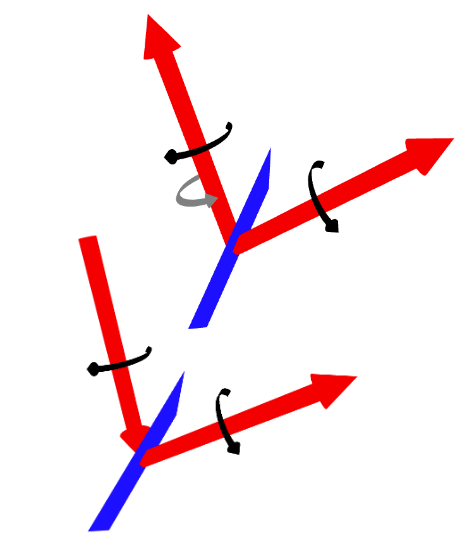
(a)

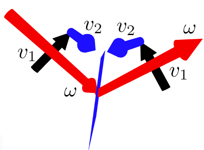
(b)

Figure 4: (a). Above: When $\omega$ (red) is reflected across a plane (blue), the corresponding rotations (black and gray arrowed arc ) are not correspondingly reflected. Bottom: To achieve the reflected rotations (black), $\omega$ should be reflected with a reversal of direction. (b). The rotation can be represented by $\omega$ or $v_{1}$(black) together with $v_{2}$ (blue). $v_{1}$ and $v_{2}$ represented the flow of the rotation. When the rotation is reflected, $v_{1}$ and $v_{2}$ are reflected.

4.2 Equivariant Frame

Instead of enforcing the above equivariance constraint on every network layer, we instead employ a subequivariant network (see Figure 2(b)) to regress a canonical frame $G$ from the preprocessed input obtained from preprocessed IMU measurements $\{(a_{i},\omega_{i})\}_{i=1}^{n}$ when dealing with $SO_{\vec{g}}(3)$ and preprocessed IMU measurements $\{(a_{i},v_{1,i},v_{2,i})\}_{i=1}^{n}$, when dealing with $O_{\vec{g}}(3)$. The canonical frame $G$ is uniquely achieved by transforming the identity frame with $R_{G}\in SO(2)$ or $O(2)$, which means we equivalently learn the transformation $R_{G}$ when we learn the equivariant frame $G$. We first convert the IMU data into $n\times C_{0}^{s}$ rotation invariant scalar features, and $n\times 2\times C_{0}^{v}$ rotation equivariant vector features, and process them jointly, taking inspiration from [44], which shows that learning from invariant features alongside vector inputs can produce universally equivariant outputs. As vector features we select the $xy$-components of each input vector ($C_{0}^{v}=2$ for $SO(2)$ and $C_{0}^{v}=3$ for $O(2)$). Instead, as scalar features we select (i) the z-components of each vector, (ii) the norm of the $xy$-components of each vector, and (iii) the pairwise dot-product of the $xy$-components of each vector. For $SO(2)$ we have $C_{0}^{s}=2+2+1=5$, while for $O(2)$ we have $C_{0}^{s}=3+3+3=9$.

As seen in Figure 2(a), preprocessed IMU measurements $\{(a_{i},\omega_{i})\}_{i=1}^{n}$ are mapped into equivariant frame $G$ i.e. canonicalized into invariant features $\{(a^{\prime}_{i},\omega^{\prime}_{i})\}_{i=1}^{n}$. This mapping is $a^{\prime}_{i}=\rho_{a}(R_{G}^{T})a_{i}$, and similarly for other vectors. Note that we first perform the aforementioned preprocessing when dealing with $O_{\vec{g}}(3)$. We then regress the invariant displacement $d^{\prime}$ and covariance $\Sigma^{\prime}$ on these invariant features before mapping back into the original frame, using the same canonical frame. Specifically, the invariant covariance is remapped as $\text{vec}(\Sigma)=\rho_{\Sigma}(R_{G})\Sigma$. This results in equivariant displacement $d=\rho_{d}(R_{G})d^{\prime}$ and covariance $\text{vec}(\Sigma)=\rho_{\Sigma}(R_{G})\text{vec}(\Sigma^{\prime})$. This design enables seamless integration of our equivariant network while separating the effects of transformations, leveraging traditional networks to process intrinsic data.

4.3 Basic Layers

While multilayer perceptrons and standard 1-D convolutions are employed to process scalar features, here we describe the specific linear and non-linear layers that combine scalar and vector features.

Equivariant Linear Layer

Following [44], we design a $2D$ version of vector neuron [20] to process the vector features in our network, enhancing efficiency. Following [25], we consider linear mappings $v^{\text{out}}=Wv^{\text{in}}$, with $v^{\text{in}},v^{\text{out}}\in\mathbb{R}^{2}$ and seek a basis of weights $W\in\mathbb{R}^{2\times 2}$, which satisfy $R_{2\times 2}Wv=WR_{2\times 2}v$, i.e., equivariantly transform vector features $v\in\mathbb{R}^{2}$. This relation yields the constraint

$$(R_{2\times 2}\otimes R_{2\times 2})\text{vec}(W)=\text{vec}(W),$$ (3)

Solving the above equation amounts to finding the eigenspace of the left-most matrix with eigenvalue 1. Such analysis for $R_{2\times 2}\in SO(2)$ yields $W_{SO(2)}=w_{1}I_{2\times 2}+w_{2}R_{90}$, where $R_{90}$ denotes a $90$ degree counter-clockwise rotation in 2D, and $w_{1},w_{2}\in\mathbb{R}$ are learnable weights. Similarly, for $O(2)$ we find $W_{O(2)}=w_{1}I_{2\times 2}$. Vectorizing this linear mapping to multiple input and output vector features we have the following $SO(2)$ and $O(2)$ equivariant linear layers:

$$SO(2) :\quad v^{\text{out}}=v^{\text{in}}W_{1}+R_{90}v^{\text{in}}W_{2}$$ (4)

$$O(2) :\quad v^{\text{out}}=v^{\text{in}}W_{1}$$ (5)

with $v^{\text{in}}\in\mathbb{R}^{2\times C_{\text{in}}}$, $v^{\text{out}}\in\mathbb{R}^{2\times C_{\text{out}}}$ and $W_{1},W_{2}\in\mathbb{R}^{C_{\text{in}}\times C_{\text{out}}}$. Note that the $SO(2)$ layer has twice as many parameters as the $O(2)$ layer.

We use the above linear components to design equivariant 1-D convolution layers by stacking multiple such weights into a kernel. Since the IMU data forms a time sequence, we implement convolutions across time. We visualize our Linear and Convolutional Layers in Figure 2(c) for better understanding.

Nonlinear Layer

Previous works [47, 46] propose various nonlinearities such as norm-nonlinearity, tensor-product nonlinearity, and gated nonlinearity for $SO(3)$ and $O(2)$ equivariance in an equivariant convolutional way; while Deng et al. [20] applies per-point nonlinearity for vector features only. Since we apply convolutions over time, and there is no transformation on this dimension, we don’t apply nonlinearity in a convolutional way but apply a nonlinearity pointwise. On the other hand, since our data includes both scalars and vectors unlike [20], we want to mix these two types of features. Therefore, we adapt gated nonlinearity [47] to pointwise nonlinearity. Specifically, for $n$ vector and scalar features $v^{\text{in}}\in\mathbb{R}^{n\times 2\times C},s^{\text{in}}\in\mathbb{R}^{n\times C}$, we concatenate the vector norm features $\|v^{\text{in}}\|\in\mathbb{R}^{n\times C}$ with the scalar features $s^{\text{in}}$, and run a single MLP yielding an output of size $n\times 2C$. We then split this output into new norm features $\gamma\in\mathbb{R}^{n\times C}$ and new activations $\beta\in\mathbb{R}^{n\times C}$ which we modulate with a non-linearity $s^{\text{out}}=\sigma(\beta)$. Finally, we rescale the original vector features according to the new norm. In summary, the update looks like

$$\gamma,\beta =\text{mlp}([\|v^{\text{in}}\|,s^{\text{in}}])$$ (6)

$$v^{\text{out}} =\gamma v^{\text{in}}$$ (7)

$$s^{\text{out}} =\sigma(\beta)$$ (8)

where $[.,.]$ concatenates along the feature dimension. See Figure 2(c) for more details.

4.4 Equivariant Covariance

Our loss function follows the previous work [33] as $\mathcal{L}_{MSE}(\hat{d},d)=\|d-\hat{d}\|_{2}$ in the first stage, and $\mathcal{L}_{MLE}(\hat{d},d)=(d-\hat{d})^{T}\Sigma^{-1}(d-\hat{d})$ in the second stage when $\mathcal{L}_{MSE}$ converges. TLIO [33] opted for a diagonal covariance matrix instead of parameterizing the off-diagonal elements using Pearson correlation, to enhance training stability [36]. However, such an assumption breaks the equivariance of the covariance and, therefore, breaks the invariance of $\mathcal{L}_{MLE}$. This issue arises because a rotation of the input invariably alters the covariance, preventing it from remaining diagonal consistently.

The design of the equivariant frame addresses the issue of equivariance by facilitating the transformation of invariant covariance as shown in Figure 2(a). We opt for a diagonal matrix format to predict the invariant covariance for several reasons: (1) Primarily, it forces the network to learn the equivariant frame whose axis is the principle axis of the covariance, and it can also regularize the network; (2) the off-diagonal elements in the equivariant frame can introduce ambiguity since when the frame is transformed by $R_{2\times 2}\in O(2)$, the network can predict $(R_{2\times 2}\oplus 1)^{T}\Sigma(R_{2\times 2}\oplus 1)$ to achieve invariant loss; (3) Empirically, we observe that $d_{z}$ is independent of $d_{xy}$, justifying the use of three diagonal elements to parameterize the covariance in the predicted frame.

See Appendix A.1.3 for details on covariance parameterizations.

5 Experiments

To demonstrate the effectiveness of canonicalizing the IMU data using the equivariant framework, we apply it to two types of neural inertial navigation systems: 1) end-to-end deep learning approach (RONIN), and 2) filter-based approach with a learned prior (TLIO). Both architectures take IMU samples in a gravity-aligned frame without gravity compensation as input to the neural network. While RONIN regresses only the 2D velocity, TLIO estimates orientation, position, velocity, IMU biases, and noise using an EKF which takes displacement and uncertainty predicted by a neural network as measurement update.

In this section, we train our framework applied to TLIO architecture on TLIO Dataset [33] and test on TLIO Dataset and Aria Everyday Activities (Aria) Dataset  [34]. Our method applied to RONIN is trained on RONIN [30]. RONIN, RIO’s methods, and our two frameworks are tested on the three popular pedestrian datasets RONIN [30], RIDI [52] and OxIOD [11]. We use the specific test datasets only to provide a fair comparison with prior work. See AppendixA.2 for more dataset details, and see AppendixA.3 and Figure 2(b) for more details and visualizations of the equivariant network. Further, in Section 6 we conduct extensive ablation illustrating the usefulness of modeling symmetry and validate our design choices for the subequivariant framework.

The Neural Network performance (indicated with $*$) is evaluated using three metrics: Mean Squared Error (MSE) in $m^{2}$, Absolute Translation Error (ATE) in $m$, and Relative Translation Error (RTE) in $m$. For evaluating only the NN, the trajectory is reconstructed via cumulative summation from the initial state as done in prior work. In case of TLIO architecture, we additionally evaluate the overall performance after integrating the NN with the EKF and report the ATE in $m$, RTE in $m$, and Absolute Yaw Error (AYE) in degrees. Details of these metrics are provided in the Appendix A.5. In the following text and tables, Eq F. will refer to EqNIO, i.e., the application of Equivariant Framework.

5.1 TLIO Architecture

	TLIO Dataset						Aria Dataset
Model	MSE*	ATE	ATE*	RTE	RTE*	AYE	MSE*	ATE	ATE*	RTE	RTE*	AYE
TLIO	3.242	1.812	3.722	0.500	0.551	2.376	5.322	1.285	2.103	0.464	0.521	2.073
TLIO-N	3.333	1.722	3.079	0.521	0.542	2.366	15.248	1.969	4.560	0.834	0.977	2.309
TLIO + Eq F. $\mathbf{SO(2)}$	3.194	1.480	2.401	0.490	0.501	2.428	2.457	1.178	1.864	0.449	0.484	2.084
TLIO + Eq F. $\mathbf{O(2)}$	2.982	1.433	2.406	0.458	0.478	2.389	2.304	1.118	1.850	0.416	0.465	2.059

Table 1: Neural network results (no EKF) are labeled with $*$. MSE are multiplied by 100. TLIO-N is TLIO trained without yaw augmentations. A lower error indicates a better model. A lowest values are annotated with Red, while the second lowest with Orange. Our proposed methods are in bold.

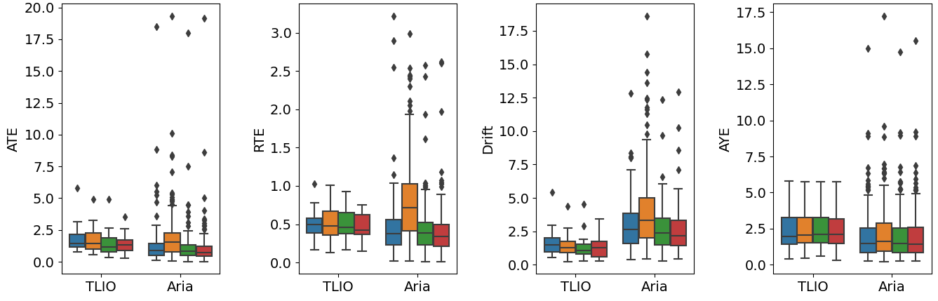
Figure 5: The superior performance of our framework applied to TLIO architecture when compared to baseline TLIO trained with and without augmentations on TLIO and Aria Datasets visualized with a box plot. Blue, Orange, Green and Red indicate TLIO, TLIO-N, TLIO+Eq F. $SO(2)$ and TLIO+Eq F. $O(2)$.

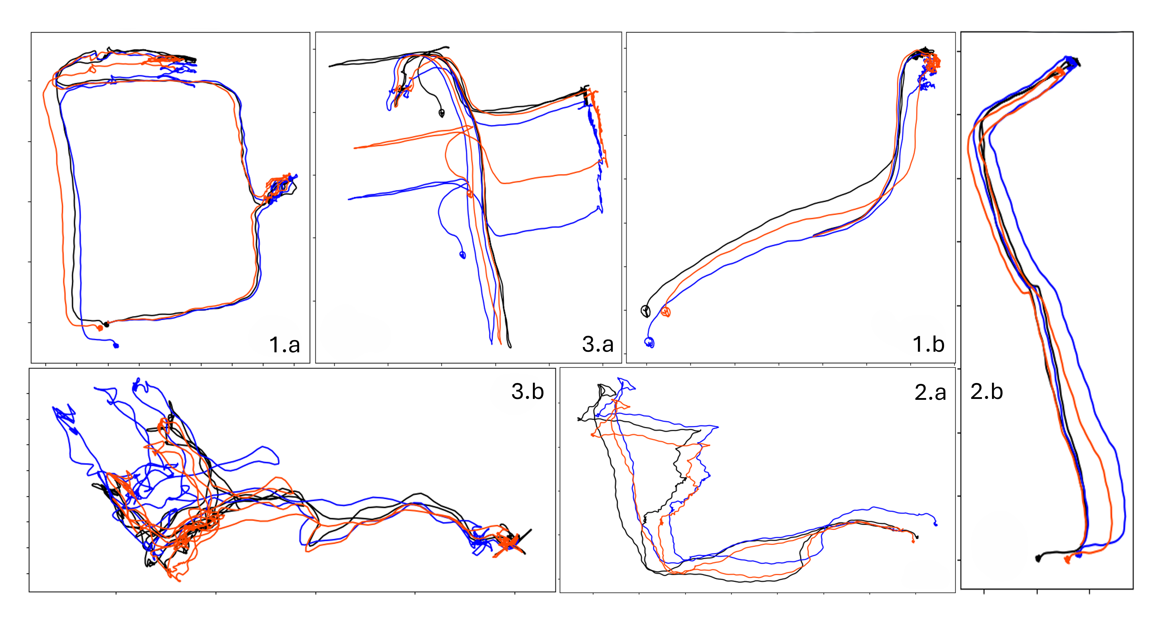
Figure 6: Visualization of final estimated trajectories on TLIO Dataset by baseline TLIO (Blue), our best method applied to TLIO (TLIO+Eq F. $O(2)$)(Red), and the Ground-Truth trajectory (Black). $1.a$ and $1.b$ are easy trajectories; $2.a$ and $2.b$ are mid-level hard trajectories; $3.a$ and $3.b$ are unusual motions not present in the training set are performed.

In Table 1, we compare baseline TLIO, trained with yaw augmentations as mentioned in their paper (termed TLIO), TLIO without the augmentation (termed TLIO-N), and our two methods applied to TLIO (termed Eq.F. $SO(2)$ and $O(2)$). As seen in Table  1, Eq F. $O(2)$ has better performance on all three metrics comparing the NN (indicated by $*$) by a large margin of 56%, 12%, and 10% with the baseline TLIO model on MSE*, ATE*, and RTE* respectively, and the Eq F. $SO(2)$ model closely follows with 56%, 11% and 7% respectively on Aria Dataset. The performance of our methods is consistent across TLIO and Aria Datasets illustrating our generalization ability. Table  1 and Figure  5 shows our method surpasses the baseline on most metrics while remaining comparable in AYE. The superior performance of our model as compared to baseline TLIO when the NN is combined with EKF (i.e., performance on ATE, RTE and AYE metrics) is attributed to its generalization ability when the orientation estimate is not very accurate as well as the equivariant covariance predicted by the network. The AYE of our method is comparable to TLIO with a difference of magnitude 0.02 degrees and the equivariant network is more tolerant to yaw perturbations. The trajectory plots for trajectories from the TLIO test dataset are seen in Figure 6 and Appendix A.6.

5.2 RONIN Architecture

	RONIN-U		RONIN-S		RIDI-T		RIDI-C		OxIOD
Model	ATE*	RTE*	ATE*	RTE*	ATE*	RTE*	ATE*	RTE*	ATE*	RTE*
RONIN-100%	5.14	4.37	3.54	2.67	1.63	1.91	1.67	1.62	3.46	4.39
RIO B-ResNet	5.57	4.38	-	-	1.19	1.75	-	-	3.52	4.42
RIO J-ResNet	5.02	4.23	-	-	1.13	1.65	-	-	3.59	4.43
RIO B-ResNet-TTT	5.05	4.14	-	-	1.04	1.53	-	-	2.92	3.67
RIO J-ResNet-TTT	5.07	4.17	-	-	1.03	1.51	-	-	2.96	3.74
RONIN + Eq F. $\mathbf{SO(2)}$	5.18	4.35	3.67	2.72	0.86	1.59	0.63	1.39	1.22	2.39
RONIN + Eq F. $\mathbf{O(2)}$	4.42	3.95	3.32	2.66	0.82	1.52	0.70	1.41	1.28	2.10

Table 2: Results for RONIN. We follow the original paper to report results with two decimal places. RONIN-U, RONIN-S, RIDI-T, RIDI-C, OxIOD refers to RONIN Unseen Dataset, RONIN Seen Dataset, RIDI Test Dataset, RIDI Cross Subject Dataset and Oxford Inertial Odometry Dataset respectively. A lower error indicates a better model. The lowest values are annotated with Red, while the second lowest with Orange. Our proposed methods are in bold.

We compare our methods applied to RONIN with the original RONIN [30], 4 methods reported by RIO [8]- RIO B-ResNet is the original RONIN model retrained, RIO J-ResNet is optimized for both MSE loss on velocity prediction and cosine similarity with an equivariance constraint modeled using an auxiliary loss, RIO B-ResNet-TTT is original RONIN model adapted at test time using Adaptive Test-Time-Training strategy, and RIO J-ResNet-TTT is RIO J-ResNet adapted at test time using Adaptive Test-Time-Training strategy. Original RONIN is trained on 100% RONIN train dataset while RIO and our methods are trained on only the publicly available 50% of RONIN train dataset. RIO does not provide results for RONIN Seen Dataset (RONIN-S) or RIDI Cross Subject Dataset (RIDI-C). As Seen in Table 2, our equivariant methods significantly outperform the original RONIN by a large margin of 14% and 9% on ATE* and RTE* respectively even on the RONIN-U dataset. Our methods have better generalization as seen on RIDI-T and OxIOD, outperforming even RIO J-ResNet-TTT by a margin of 56% and 43% on ATE* and RTE* respectively on OxIOD Dataset. The Eq F. $O(2)$ model converges at 38 epochs compared to over 100 in RONIN implying faster network convergence with our framework as compared to data augmentation used in RONIN. This demonstrates the superior generalization of our strictly equivariant architecture. RIO’s approach, involving multiple data rotations, test optimization, and a deep ensemble at test time, would result in higher computational and memory costs as compared to our method.

6 Ablation Study

	TLIO Dataset						Aria Dataset
Model	MSE*	ATE	ATE*	RTE	RTE*	AYE	MSE*	ATE	ATE*	RTE	RTE*	AYE
TLIO	3.242	1.812	3.722	0.500	0.551	2.376	5.322	1.285	2.102	0.464	0.521	2.073
TLIO-N	3.333	1.722	3.079	0.521	0.542	2.366	15.248	1.969	4.560	0.834	0.977	2.309
Deeper TLIO	3.047	1.613	2.766	0.524	0.519	2.397	2.403	1.189	2.541	0.472	0.540	2.081
TLIO-NQ	3.008	1.429	2.443	0.495	0.496	2.411	2.437	1.213	2.071	0.458	0.508	2.096
TLIO-PCA	3.473	1.506	2.709	0.523	0.535	2.459	6.558	1.717	4.635	0.771	0.976	2.232
Eq CNN	3.194	1.580	3.385	0.564	0.610	2.394	8.946	3.223	6.916	1.091	1.251	2.299
TLIO + Eq F. $SO(2)$+S	3.331	1.626	2.796	0.524	0.536	2.440	2.591	1.146	2.067	0.466	0.517	2.089
TLIO + Eq F. $SO(2)$+P	3.298	1.842	2.652	0.588	0.523	2.537	2.635	1.592	2.303	0.585	0.539	2.232
TLIO + Eq F. $\mathbf{SO(2)}$	3.194	1.480	2.401	0.490	0.501	2.428	2.457	1.178	1.864	0.449	0.484	2.084
TLIO + Eq F. $O(2)$+S	3.061	1.484	2.474	0.462	0.481	2.390	2.421	1.175	1.804	0.421	0.458	2.043
TLIO + Eq F. $O(2)$+P	2.990	1.827	2.316	0.578	0.478	2.534	2.373	1.755	1.859	0.564	0.468	2.223
TLIO + Eq F. $\mathbf{O(2)}$	2.982	1.433	2.406	0.458	0.478	2.389	2.304	1.118	1.849	0.416	0.465	2.059

Table 3: Ablation Studies. TLIO-NQ is TLIO with non-equivariant frames. TLIO-PCA is TLIO using PCA to predict handcrafted frames. TLIO-N is TLIO trained without yaw augmentations. Eq F. $\bm{SO(2)}$+S is Equivaraiant frame with circular covariance. Eq F. $\bm{SO(2)}$+P is $SO(2)$ equivariant networks with pearson parameterized covariance. Eq CNN is fully equivariant CNN. The same naming conventions apply to the $O(2)$ variants. A lower error indicates a better model. The lowest values are annotated with Red, followed by Orange and Yellow respectively. Our proposed methods are in bold.

In this section, we investigate and motivate the necessity for incorporating equivariance in inertial odometry, the choice of equivariant architecture and covariance. We present all the ablation on TLIO in Table 3 for the neural network and the overall performance when NN is integrated with the EKF. Appendix A.7 contains the results of evaluating all the above models separately on a test dataset augmented with rotations and/or reflections. Appendix A.10 presents the ablation on IMU input sequence length and lastly, in Appendix A.11 we present sensitivity analysis to gravity direction using 5 discrete angles.

Baseline Ablation: Is yaw augmentation needed when the input is in a local gravity-aligned frame? We trained TLIO both with and without yaw augmentation using identical hyperparameters and the results in Table 3 revealed that augmentation enhances the network’s generalization, improving all metrics for the Aria dataset with the lowest margin of 10% on AYE and highest margin of 65% for MSE*. This underscores the importance of equivariance for network generalization. Does a Deeper TLIO with a comparable number of parameters match the performance of equivariant methods? We enhanced the residual depth of the original TLIO architecture from 4 residual blocks of depth 2 each to 4 residual blocks with depth 3 each to align its number of parameters with our Eq F. $SO(2)$ model. Despite having fewer parameters due to the removal of the orthogonal basis in the $SO(2)$ vector neuron-based architecture, the Eq F. $O(2)$ model still outperformed the augmented TLIO. The data from Table 3 demonstrate that merely increasing the network’s size, without integrating true equivariance, is insufficient for achieving precise inertial odometry.

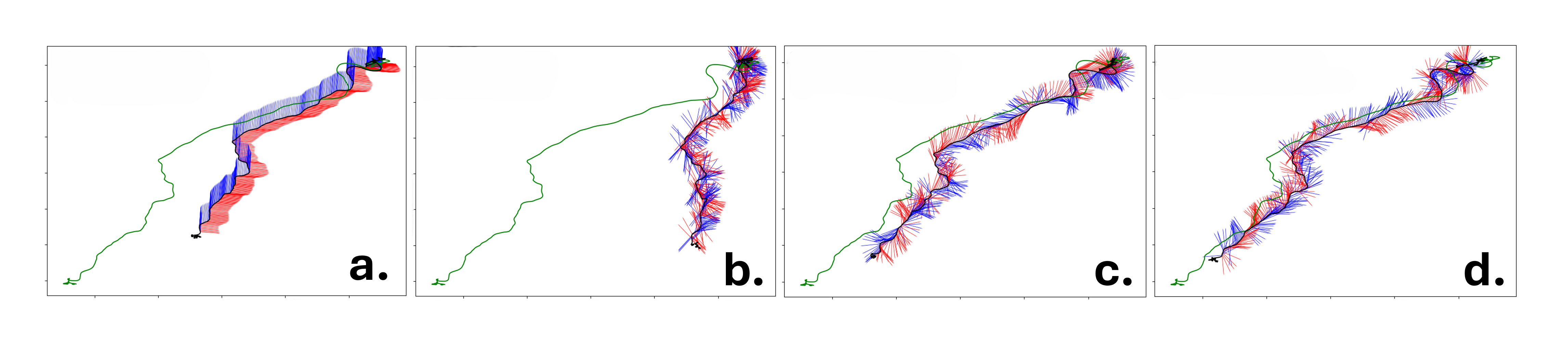
Figure 7: Visualization of one neural integrated trajectory in the Aria Dataset: the green trajectory shows the ground truth, the black trajectories show predictions, and the blue and red vectors represent the predicted frame’s basis vectors. a) Non-equivariant MLP b) PCA c) Eq F. SO(2) d) Eq F. O(2)

Frame Ablation: Can a non-equivariant MLP predict meaningful frames? We trained TLIO with augmentation and identical hyperparameters alongside an additional MLP mirroring the architecture of our method to predict a frame and term this baseline TLIO-NQ. We observed that TLIO-NQ tends to overfit to the TLIO dataset, and the predicted frames were not meaningful, as illustrated in Figure 7. Can frames predicted using PCA (handcrafted equivariant frame) achieve the same performance? PCA frames underperform on the Aria dataset and perform worse than the original TLIO, likely due to PCA’s noise sensitivity and the production of non-smooth frames, as shown in Figure 7. Additionally, PCA cannot distinguish between $SO(2)$ and $O(2)$ transformations. Figure 7 also shows that $O(2)$ does not have frames as smooth as $SO(2)$ as the reflected bends have reflected frames.

Architecture Ablation: Does a fully equivariant architecture perform better than our frame-based approach ? We trained a fully equivariant convolutional network using the basic layers described in Section 4.3. As shown in Table 3, our frame-based methods are more effective and efficient than the equivariant CNN. We believe the fully equivariant architecture is overly restrictive, while our approach leverages the power of scalars and conventional backbones. Additionally, our method integrates easily with any state-of-the-art neural inertial navigation system, unlike the fully equivariant architecture, which requires redesigning.

Covariance Ablation: Do we need equivariant covariance? We investigated the importance of equivariant covariance for both $SO(2)$ and $O(2)$ groups, as described in Section 4.4( See Appendix A.1.3 for more details on covariance parameterizations.). In Table 3, the models Eq F. $SO(2)$+S and Eq F. $O(2)$+S are trained with invariant covariance. The results show that equivariant covariance yields better performance, especially when combined with EKF, as it provides a more accurate estimate of the measurement covariance. Can a full covariance matrix predicted via Pearson parameterization further improve the performance? In Table 3, Eq F. $SO(2)$+P and Eq F. $O(2)$+P are outperformed by our model in most cases. As mentioned in Section 4.4, this experimental result indicates that by aligning the principle axis of the covariance into the basis of the equivariant frame, we intrinsically force the covariance in the equivariant frame to be diagonal, which reduces the ambiguity while training. Prediction of diagonal covariance improves stabilization and convergence in the optimization process as stated in TLIO. The visualization of covariance consistency of our Eq F. $O(2)$ model is in Appendix A.9.

7 Limitations

Similarly to previous works such as TLIO and RONIN, our framework employs gravity-aligned frames. This assumption reduces the problem from full $O(3)$ equivariance to $O(2)$ subequivariance. In reality, this alignment depends on the accuracy of the estimated gravity vector. However, the effectiveness of this approach hinges on the precision of the estimated gravity vector. Given that our data preprocessing incorporates ground truth estimates, inaccuracies in gravity alignment may lead to errors in predicted displacement, velocities, and covariance measures.

Another limitation is the robustness of the method against unseen motions. While our focus was on enhancing generalization across unseen rotations and reflections, we did not address the network’s sensitivity to unexpected motion patterns, such as sudden jerks or free falls. Moreover, generalizing networks trained on one hardware platform to another remains a challenge. We leave these aspects to our future work.

8 Conclusion

We introduce an equivariant framework designed for neural IMUs. Our method robustly estimates the equivariant frame, capturing the inherent symmetry of IMU input data. Our theoretical framework enforces $O(2)$ subequivariance in both the predicted velocity/displacement and the predicted covariance. We applied this framework to the TLIO and RONIN architectures and benchmarked it on various datasets. Our results show improved performance compared to networks using only data augmentation, advancing the state-of-the-art for neural integration of IMU data. This work further highlights the effectiveness of equivariant networks in overcoming generalization challenges.

Appendix A Appendix

A.1 Preliminary

A.1.1 Equivariance

In this section, we introduce more preliminaries of group and representation theory which form the mathematical tools for equivariance.

Group

The group $G$ is a set equipped with an associative binary operation $\cdot$ which maps two arbitrary two elements in $G$ to an element in $G$. It includes an identity element, and every element in the set has an inverse element.

In this paper, we focus on the group $SO(2)$ and $O(2)$. $SO(2)$ is the set of all 2D planar rotations, represented by 2x2 orthogonal matrices with determinant 1. This group operation is matrix multiplication, and each rotation matrix has an inverse, which is its transpose. The identity element is the matrix representing no rotation.

$O(2)$ consists of all distance-preserving transformations in Euclidean 2D space, including both rotations and reflections. Elements of $O(2)$ are 2x2 orthogonal matrices, with the group operation being matrix multiplication. Each transformation matrix has an inverse, and the identity element is the matrix representing no transformation.

Group Representation and Irreducible Representation

Group representation is a homomorphism from the group $G$ to the general linear map of a vector space $V$ of a file $K$, denoted $GL(V)$.

An irreducible representation (irrep) of a group $G$ is a representation in which the only invariant subspaces under the action of $G$ are the trivial subspace $\{\bm{0}\}$ and the entire space $V$. In other words, an irreducible representation cannot be broken down into smaller, nontrivial representations,i.e., it cannot be the direct sum of several nontrivial representations.

For $SO(2)$, we can use $\theta\in(0,2\pi]$ to represent $SO(2)$, for any $\theta$, the irreducible representation of the frequency $n\in\mathbb{N}$ is:

$$\rho_{n}(\theta)=\begin{pmatrix}\cos n\theta&-\sin n\theta\\ \sin n\theta&\cos n\theta\end{pmatrix}.$$

For $O(2)$, we can use $r\in\{-1,1\}$ to denote reflection and $\theta\in(0,2\pi]$ to denote rotation. The trivial representation $\rho_{0}(r,\theta)=1$. For the nontrivial representation of frequency $n\in\mathbb{N}^{+}$

$$\rho_{n}(r,\theta)=\begin{pmatrix}\cos(n\theta)&-\sin(n\theta)\\ \sin(n\theta)&\cos(n\theta)\end{pmatrix}\begin{pmatrix}1&0\\ 0&r\end{pmatrix}$$

There is another one-dimensional irreps for $O(2)$, $\rho(r,\theta)=r$ which corresponds to the trivial representation of rotation.

The introduction to group representations has been covered extensively in previous work on equivariance [16, 47, 51]. Specifically, for $SO(2)$ and $O(2)$, Weiler and Cesa [46] provide a detailed introduction.

Invariance and Equivariance

Given a network $\Phi:\mathcal{X}\rightarrow\mathcal{Y}$, if for any $x\in\mathcal{X}$,

$$\Phi(\rho^{\mathcal{X}}x)=\Phi(x),$$

implies the group representation $\rho^{\mathcal{Y}}$ of the output space is trivial, i.e. identity, and the input does not transform (i.e. the input is invariant) under the action of the group. In our paper, the coordinates/ projections of $3D$ vector to the gravity axis $z$-axis are invariant, therefore we call them invariant scalars.

A network $\Phi:\mathcal{X}\rightarrow\mathcal{Y}$ is equivariant if it satisfies the constraint

$$\Phi(\rho^{\mathcal{X}}x)=\rho^{\mathcal{Y}}\Phi(x).$$

In this paper, when the output is displacement the $z-$ component is invariant while $xy-$ components are acted under the representation of $\rho_{1}$ defined in the above section. Hence, for displacement, $\rho^{\mathcal{Y}}=\rho_{1}\oplus 1$ and for covariance $3D$ covariance, $\rho^{\mathcal{Y}}=(\rho_{1}\oplus 1)\otimes(\rho_{1}\oplus 1)$

Subequivariance

As mentioned in prior works [15, 28], the existence of gravity breaks the symmetry in the vertical direction, reducing O(3) to its subgroup O(2). We formally characterize this phenomenon of equivariance relaxation as subequivariance. We have mathematically defined the subequivariance in Section 3 of the paper. In simpler terms, the gravity axis is decoupled and treated as an invariant scalar while the other two axes are handled as a separate 2D vector. Upon rotation, the invariant scalar remains constant while the other two axes are transformed under rotation. So we are limited now to SO(2) rotations and roto-reflections. In the general case of equivariance, the 3D vector would be considered three-dimensional and an SO(3) rotation would act on it. The transformation would be along all three axes.

A.1.2 Inertial Odometry

In this section, we introduce more preliminaries on the terms used in inertial odometry.

Inertial Measurement Unit

Inertial Measurement Unit (IMU) is an electronic device that measures and reports linear acceleration, angular velocity, orientation, and other gravitational forces. An IMU typically consists of a 3-axis accelerometer, a 3-axis gyroscope, and depending on the heading requirement a 3-axis magnetometer.

An accelerometer measures instantaneous linear acceleration ($a_{i}$). It can be thought of as a mass on a spring, however in micro-electro-mechanical systems (MEMS) it is beams that flex instead of spring.

A gyroscope measures instantaneous angular velocity ($\omega_{i}$). It measures the angular velocity of its frame, not any external forces. Traditionally, this can be measured by the fictitious forces that act on a moving object brought about by the Coriolis effect, when the frame of reference is rotating. In MEMs, however, we use high-frequency oscillations of a mass to capture angular velocity readings by the capacitance sense cones that pick up the torque that gets generated.

World Frame

A world frame, also known as a cartesian coordinate frame, is a fixed frame with a known location and does not change over time.

Gravity-aligned World Frame

When the world frame has one of its axes perfectly aligned with the gravity vector, it is said to be a gravity-aligned world frame. In this paper, we denote this frame with $w$.

Local-gravity-aligned Frame

A local-gravity-aligned frame has one of its axes aligned with the gravity vector at all times but it is not fixed to a known location.

Body Frame

A body frame comprises the origin and orientation of the object described by the navigation solution. In this paper, the body frame is the IMU’s frame. This is denoted as $i$ for the IMU data.

Gravity-compensation

Gravity compensation refers to the removal of the gravity vector from the accelerometer reading.

Gravity-alignment

Gravity-alignment of IMU data refers to expressing the data in the gravity-aligned frame. This is done by aligning the z-axis of the IMU inertial frame with the gravity vector pointing downwards and is usually achieved by fixing the roll and pitch (rotations around the x and y axes) or by applying a transformation estimated by the relative orientation between the gravity vector and a fixed z-axis pointing downwards. This is usually achieved with a simple rotation.

A.1.3 Uncertainty Quantification in Inertial Odometry

In this section, we provide more context on uncertainty quantification in odometry and detail the different parameterizations used for regressing the covariance matrix in the paper.

Homoscedastic Uncertainty

Homoscedatic uncertainty refers to uncertainty that does not vary for different samples, i.e., it is constant.

Heteroscedastic Uncertainty

Heteroscedastic uncertainty is uncertainty that is dependent on the sample, i.e., it varies from sample to sample.

Epistemic Uncertainty

Epistemic uncertainty is uncertainty in model parameters. This can be reduced by training the model for longer and/or increasing the training dataset to include more diverse samples.

Aleatoric Uncertainty

Aleatoric uncertainty is the inherent noise of the samples. This cannot be reduced by tuning the network or increasing the diversity of the data.

Why do we need to estimate uncertainty in inertial odometry?

In inertial odometry when we use a probabilistic filter-based approach like a Kalman Filter, the filter estimates the probability distribution over the pose recursively. While integrating the neural network prediction, the filter fuses the prediction with other sensor measurements, like raw IMU data in TLIO [33], by weighing it based on the accuracy or reliability of the measurements. For neural networks, this reliability is obtained by estimating the uncertainty. If we use a fixed uncertainty (homoscedastic) it is seen to cause catastrophic failures of perception systems. The uncertainty estimated in TLIO captures the extend to which input measurements encode the motion model prior.

What is the uncertainty we are estimating in inertial odometry?

We are regressing aleatoric uncertainty using the neural network and training the model till the epistemic uncertainty is very small as compared to aleatoric uncertainty.

How is the uncertainty estimated in this paper?

We regress aleatoric uncertainty as a covariance matrix jointly while regressing 3D displacement following the architecture of TLIO [33]. Since there is no ground truth for the covariance, we use the negative log-likelihood loss of the prediction using the regressed Gaussian distribution. As this loss captures the Mahalanobis distance, the network gets jointly trained to tune the covariance prediction. We do not estimate epistemic uncertainty separately in this paper, but as mentioned in Russell and Reale [36] we train the network until the epistemic uncertainty is small as compared to aleatoric uncertainty.

Diagonal covariance matrix

TLIO [33] regresses only the three diagonal elements of the covariance matrix as log $\sigma_{xx}$, log $\sigma_{yy}$ and log $\sigma_{zz}$ and the off-diagonal elements are zero. This formulation assumes the axes are decoupled and constrains the uncertainty ellipsoid to be along the local gravity-aligned frame.

Full covariance matrix using Pearson correlation

Russell and Reale [36] define a parameterization to regress the full covariance matrix. They regress six values of which three are the diagonal elements log $\sigma_{xx}$, log $\sigma_{yy}$ and log $\sigma_{zz}$ and the remaining three are Pearson correlation coefficients $\rho_{xy}$, $\rho_{yz}$, and $\rho_{xz}$. The diagonal elements are obtained by exponential activation while the off-diagonal elements are computed as follows

$$\Sigma_{ij}=\rho_{ij}\sigma_{i}\sigma_{j}$$

where $\rho_{ij}$ passes through tanh activation.

Diagonal covariance matrix in canonical frame

In our approach we regress the three diagonal elements as log $\sigma_{xx}$, log $\sigma_{yy}$ and log $\sigma_{zz}$ in the invariant canonical frame. Since the z-axis is decoupled from the xy-axis, only $\sigma_{xx}$ and $\sigma_{yy}$ are back-projected using the equivariant frame to obtain a full 2D covariance matrix from the diagonal entries. The resulting matrix is as follows

$$\begin{bmatrix}\sigma_{xx}&\sigma_{xy}&0\\ \sigma_{xy}&\sigma_{yy}&0\\ 0&0&\sigma_{zz}\end{bmatrix}$$

A.2 Dataset Details

In this section, we provide a detailed description of the 4 datasets used in this work - TLIO and Aria for TLIO architecture, and RONIN, RIDI and OxIOD for RONIN architecture.

TLIO Dataset-

The TLIO Dataset [33] is a headset dataset that consists of IMU raw data at 1kHz and ground truth obtained from MSCKF at 200 Hz for 400 sequences totaling 60 hours. The ground truth consists of position, orientation, velocity, IMU biases and noises in $\mathbb{R}^{3}$. The dataset was collected using a custom rig where an IMU (Bosch BMI055) is mounted on a headset rigidly attached to the cameras. This dataset captures a variety of activities including walking, organizing the kitchen, going up and down stairs, on multiple different physical devices and more than 5 people for a wide range of individual motion patterns, and IMU systematic errors. We use their data splits for training (80%), validation (10%), and testing(10%).

Aria Everyday Dataset-

Aria Everyday Dataset [34] is an open-sourced egocentric dataset that is collected using Project Aria Glasses. This dataset consists of 143 recordings accumulating to 7.3 hrs capturing diversity in wearers and everyday activities like reading, morning exercise, and relaxing. There are two IMUs on the left and right side of the headset of frequencies 800 and 1kHz respectively. They have two sources of ground truth- open and closed loop trajectory at 1kHz. Open loop trajectory is strictly causal while closed loop jointly processes multiple recordings to place them in a common coordinate system. The ground truth contains position and orientation in $\mathbb{R}^{3}$. We use it as a test dataset. The raw right IMU data is used to compare closed-loop trajectory with EKF results. The data was downsampled to 200Hz and preprocessed using the closed-loop trajectory to test the Neural Network trained on TLIO.

RONIN Dataset-

RONIN Dataset [30] consists of pedestrian data with IMU frequency and ground truth at 200Hz. RONIN data features diverse sensor placements, like the device placed in a bag, held in hand, and placed deep inside the pocket, and multiple Android devices from three vendors Asus Zenfone AR, Samsung Galaxy S9 and Google Pixel 2 XL. Hence, this dataset has different IMUs depending on the vendor. We use RONIN data splits to train and test their model with and without our framework.

RIDI Dataset-

RIDI Dataset [52] is another pedestrian dataset with IMU frequency and ground truth at 200 Hz. This dataset features specific human motion patterns like walking forward/backward, walking sidewards, and acceleration/deceleration. They also record data with four different sensor placements. We report test results of RONIN models on both RIDI test and cross-subject datasets. RIDI results are presented after post-processing the predicted trajectory with the Umeyama algorithm [43] for fair comparison against other methods.

OxIOD Dataset-

OxIOD Dataset [11] stands for Oxford Inertial Odometry Dataset consists of various device placements/attachments, motion modes, devices, and users capturing everyday usage of mobile devices. The dataset contains 158 sequences totaling 42.5 km and 14.72 hours captured in a motion capture system. We use their unseen multi-attachments test dataset for evaluating our framework applied to RONIN architecture.

A.3 Equivariant Network Implementation Details

In this section, we describe in detail the equivariant network implementation and how it is combined with TLIO and RONIN. The input to the framework is IMU samples from the accelerometer and gyroscope for a window of 1s with IMU frequency 200Hz resulting in $n$ = 200 samples. All IMU samples within a window are gravity-aligned with the first sample at the beginning of the window, previously referred to as the clone state. The network design, as seen in Figure 2(b) and Figure 2(c), differs in architecture for $SO(2)$ and $O(2)$ and hence described separately below.

$SO(2)$-

We decouple the z-axis from the other two axes and treat linear acceleration and angular velocity along the z-axis as scalars (2). We also take the norm of the 2D accelerometer and gyroscope measurements (2), their inner product (1) resulting in invariant scalars $\mathbb{R}^{n\times 5}$. The x and y components of IMU measurements are passed as vector inputs $\mathbb{R}^{n\times 2\times 2}$. The vectors and scalars are then separately passed to the linear layer described in Section 4.3. The equivariant network predicting the equivariant frame consists of 1 linear layer, 1 nonlinearity, 1 convolutional block with convolution applied over time, non-linearity, and layer norm. The hidden dimension is 128 and the convolutional kernel is 16 x 1. Finally, the fully connected block of hidden dimension 128 and consisting of linear, nonlinearity, layer norm, and output linear layer follows a pooling over the time dimension. The output of the final linear layer is 2 vectors representing the two bases of the equivariant frame. The input vectors of dimension $\mathbb{R}^{n\times 2\times 2}$ are projected into the invariant space via the equivariant frame resulting in invariant features in $\mathbb{R}^{n\times 4}$. These features are combined with the input scalars and passed as input ($\mathbb{R}^{n\times 6}$) to TLIO or RONIN base architecture. The output of TLIO is invariant 3D displacement and diagonal covariance along the principal axis. The output of RONIN is 2D velocity. The x and y components are back-projected using the equivariant frame to obtain displacement vector d in $\mathbb{R}^{2}$ and the covariance in the original frame. The covariance is parameterized and processed as mentioned in Section 4.4.

$O(2)$-

The preprocessing is as described in Section 4.1 where $\omega$ is decomposed to two vectors $\textit{v}_{1}$ and $\textit{v}_{2}$ that have magnitude $\lvert\omega\rvert$. The preprocessed input therefore consists of 3 vectors a, $\textit{v}_{1}$ and $\textit{v}_{2}$. This is then passed to the equivariant network by decoupling the z-axis resulting in vector input $\mathbb{R}^{n\times 3\times 2}$ which represents 3 vectors in 2D. The scalars passed to the linear layer described in Section 4.3 consist of the accelerometer z-axis measurement (1), the z component of the two vectors $v_{1}$ and $v_{2}$ (2), the norm of the vectors (3) and the inner product of the vectors(3) resulting in $\mathbb{R}^{n\times 9}$. The network architecture is the same as $SO(2)$ with hidden dimension 64 and 2 convolutional blocks in order to make it comparable in the number of parameters to $SO(2)$ architecture. The invariant features obtained by projecting the three vectors using the equivariant frame are processed as mentioned in Section 4.1 to obtain 2 vectors in 3D that are fed as input to TLIO and RONIN. The postprocessing is the same as $SO(2)$.

The framework is implemented in Pytorch and all hyperparameters of the base architectures are used to train TLIO and RONIN respectively. The $SO(2)$ architecture has 1821312 while $O(2)$ has 2378368 number of parameters and the base TLIO architecture has 5424646. The baseline TLIO and our methods applied to TLIO were trained on NVIDIA a40 GPU occupying 7-8 GB memory per epoch. The training took 5 mins per epoch over the whole training dataset. We train for 10 epochs with MSE Loss and the remaining 40 epochs with MLE Loss similar to TLIO [33]. RONIN was trained on NVIDIA 2080ti for 38 epochs taking 2 mins per epoch. The loss function used was MSE as mentioned in Herath et al. [30]. The EKF described in TLIO was run on NVIDIA 2080ti with the same initialization and scaling of predicted measurement covariance as in TLIO [33].

We compare the resource requirements of the SO(2), and O(2) variant of our method coupled with TLIO, with base TLIO without an equivariant frame. We report the floating point operations (FLOPs), the inference time (in milliseconds), and Maximum GPU memory (in GB) during inference, on an NVIDIA 2080 Ti GPU for the neural network averaged over multiple runs to get accurate results. While base TLIO uses 35.5 MFLOPs, 3.5 ms, and 0.383 GB per inference, our SO(2) equivariant method instead uses 531.9 MFLOPs, 4.3 ms, and 0.383 GB per inference. Finally, our O(2) equivariant method uses 638.5 MFLOPs, 4.6 ms, and 0.385 GB per inference. We further evaluate the Maximum GPU memory for the equivariant networks separately and report 0.255 GB per inference for SO(2) equivariant frame prediction and 0.257 GB per inference for O(2) equivariant frame prediction. The Maximum GPU memory is unaffected because the equivariant frame computation utilizes less memory than TLIO.

Finally, we also evaluate our method with a downstream EKF on an NVIDIA 2080 Ti GPU. The EKF incorporates raw IMU measurements for propagation, and displacement measurements from the neural network as measurement updates. For every 20 imu samples, we send the last 200 IMU measurements to the neural network to provide this measurement update. The original TLIO requires 0.492 seconds and 1.113 GB of memory. For the SO(2) variant of our method, we require 0.554 seconds and 1.109 GB of memory to process 1 second of real-world data. For the O(2) variant, we use 0.554 seconds and 1.115 GB of memory, showing that our method is faster than real-time. The increase in memory for the O(2) variant is due to the additional preprocessing step.

With comparable computing resources, our equivariant model outperforms TLIO since we leverage symmetry, which is an intrinsic property in inertial odometry.

A.4 EKF Details

A.4.1 Process Model

The EKF filter states include orientation, translation, velocity, biases of the imu body. The EKF propagation uses raw IMU samples in the local IMU frame, following strap-down inertial kinematics equations:

$$\small\mathbf{\prescript{w}{i}{\hat{R}_{k+1}}}=\mathbf{\prescript{w}{i}{\hat{R}_{k}}}\exp_{SO(3)}(\mathbf{(\omega_{k}-\hat{b}_{gk})}\Delta t)$$

$$\mathbf{\prescript{w}{}{\hat{v}_{k+1}}}=\mathbf{\prescript{w}{}{\hat{v}_{k}}}+\mathbf{\prescript{w}{}{g}}\Delta t+\mathbf{\prescript{w}{i}{\hat{R}_{k}}(a_{k}-\hat{b}_{ak})}\Delta t$$

$$\mathbf{\prescript{w}{}{\hat{p}_{k+1}}}=\mathbf{\prescript{w}{}{\hat{p}_{k}}}+\mathbf{\prescript{w}{}{\hat{v}_{k}}}\Delta t+\frac{1}{2}\Delta t^{2}(\mathbf{\prescript{w}{}{g}+\mathbf{\prescript{w}{i}{\hat{R}_{k}}}(a_{k}-\hat{b}_{a}k)})$$

$$\mathbf{\hat{b}_{g(k+1)}=\hat{b}_{gk}+\eta_{gdk}}$$

$$\mathbf{\hat{b}_{a(k+1)}=\hat{a}_{gk}+\eta_{adk}}$$

where at timestep k, $\prescript{w}{i}{\hat{R}_{k}}$ is the orientation estimate of the Kalman filter from IMU frame to the gravity-aligned world frame, $\hat{b}_{gk}$ are the gyroscope biases, $\Delta t$ is the time interval, $\prescript{w}{}{\hat{v}_{k}}$ is the velocity estimate, $\prescript{w}{}{g}$ is the constant gravity vector, $\hat{b}_{ak}$ are the accelerometer biases, $\prescript{w}{}{\hat{p}_{k}}$ is the position estimate, $\eta_{gdk}$ and $\eta_{adk}$ are the IMU noises that are assumed to be normally distributed.

A.4.2 Measurement Model

The measurement model in the EKF uses the displacement estimates provided by the neural network, aligning them in a local gravity-aligned frame to ensure the measurements are decoupled from global yaw information:

$$\hat{h}(\mathbf{X})=\mathbf{R}_{\gamma}^{T}(\mathbf{p}_{j}-\mathbf{p}_{i})=\hat{d}_{ij}+\eta_{ij}$$

where $\mathbf{R}_{\gamma}$ is the yaw rotation matrix, $\mathbf{p}_{i}$ and $\mathbf{p}_{j}$ are positions of the past and current states, and $\eta_{ij}$ represents the measurement noise modeled by the network’s uncertainty output.

A.4.3 Update Model

The Kalman gain is computed based on the measurement and covariance matrices, and the state and covariance are updated accordingly. The key update equations involve the computation of the Kalman gain ($\mathbf{K}$), updating the state ($\mathbf{X}$), and updating the covariance matrix ($\mathbf{P}$):

$$\mathbf{K}=\mathbf{P}\mathbf{H}^{T}(\mathbf{H}\mathbf{P}\mathbf{H}^{T}+\Sigma)^{-1}$$

$$\mathbf{X}=\mathbf{X}+\mathbf{K}(\hat{h}(\mathbf{X})-\hat{d}_{ij})$$

$$\mathbf{P}=(\mathbf{I}-\mathbf{K}\mathbf{H})\mathbf{P}$$

A.5 Evaluation Metrics Definition

We follow most metrics in TLIO [33] and RONIN [30], besides $MSE$ loss we reported in the paper. Here we provide the mathematical details of these metrics.

• MSE (m²): Translation error per sample between the predicted and ground truth displacement averaged over the trajectory. It is computed as $\frac{1}{n}\sum^{n}_{i}\|\prescript{w}{}{p}_{i}-\prescript{w}{}{\hat{p}}_{i}\|$. However, it should be noted that MSE mentioned in TLIO [33] is the same as MSE Loss calculated as the squared error averaged separately for each axis $\frac{1}{n}\sum^{n}_{i}\|\prescript{w}{}{p}_{i,r}-\prescript{w}{}{\hat{p}}_{i,r}\|$ where r is an axis.

• ATE (m): Translation Error assesses the discrepancy between predicted and ground truth (GT) positions across the entire trajectory. It is computed as $\sqrt{\frac{1}{n}\sum^{n}_{i}\|\prescript{w}{}{p}_{i}-\prescript{w}{}{\hat{p}}_{i}\|}$

• RTE (m): Following the method described in [16], Relative Translation Error measures the local differences between predicted and GT positions over a specified time window of duration $\delta t$ (1 minute). $\sqrt{\frac{1}{n}\sum^{n}_{i}\|\prescript{w}{}{p}_{i+\delta t}-\prescript{w}{}{p}_{i}-(\prescript{w}{}{\hat{p}}_{i+\delta t}-\prescript{w}{}{\hat{p}}_{i})\|}$.

• AYE Absolute Yaw Error is calculated as $\sqrt{\frac{1}{n}\sum^{n}_{i}\|\gamma_{i}-\hat{\gamma}_{i}\|}$.

A.6 Visualization of TLIO results

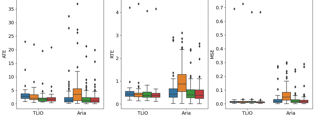
Figure 8: The superior performance of our framework applied to TLIO architecture when compared to baseline TLIO trained with and without augmentations on TLIO and Aria Datasets visualized with a box plot. Blue, Orange, Green and Red indicate TLIO, TLIO-N, TLIO+Eq F. $SO(2)$ and TLIO+Eq F. $O(2)$. ATE, RTE and MSE indicate ATE*, RTE* and MSE* corresponding to only the NN results.

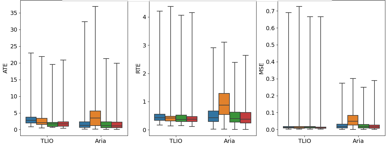
Figure 9: The superior performance of our framework applied to TLIO architecture when compared to baseline TLIO trained with and without augmentations on TLIO and Aria Datasets visualized with a box plot. Blue, Orange, Green and Red indicate TLIO, TLIO-N, TLIO+Eq F. $SO(2)$ and TLIO+Eq F. $O(2)$. ATE, RTE and MSE indicate ATE*, RTE* and MSE* corresponding to only the NN results. The whisker is extended to 1.5 * IQR (inter-quartile range).

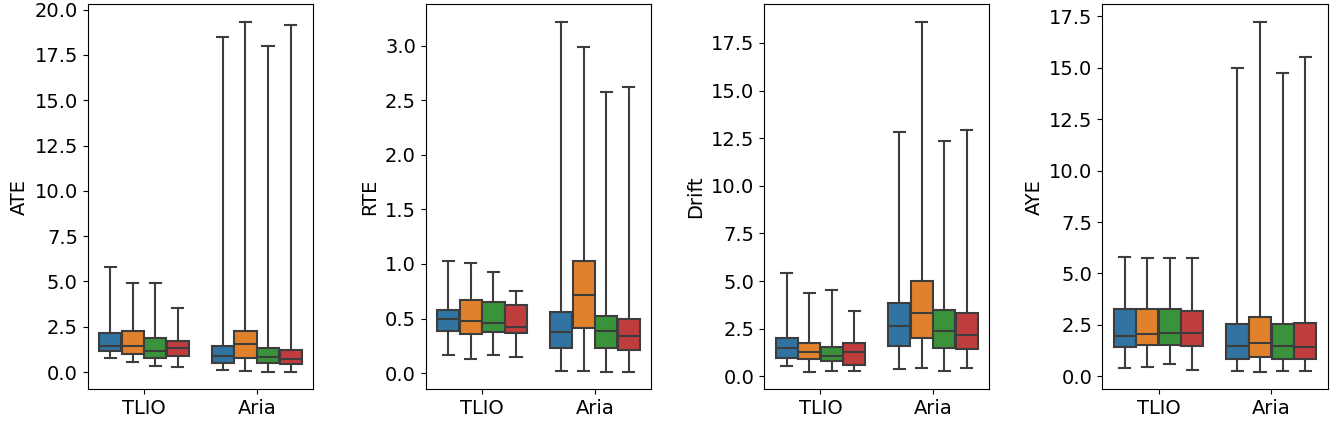
Figure 10: The superior performance of our framework applied to TLIO architecture when compared to baseline TLIO trained with and without augmentations on TLIO and Aria Datasets visualized with a box plot. Blue, Orange, Green and Red indicate TLIO, TLIO-N, TLIO+Eq F. $SO(2)$ and TLIO+Eq F. $O(2)$. The whisker is extended to 1.5 * IQR (inter-quartile range).

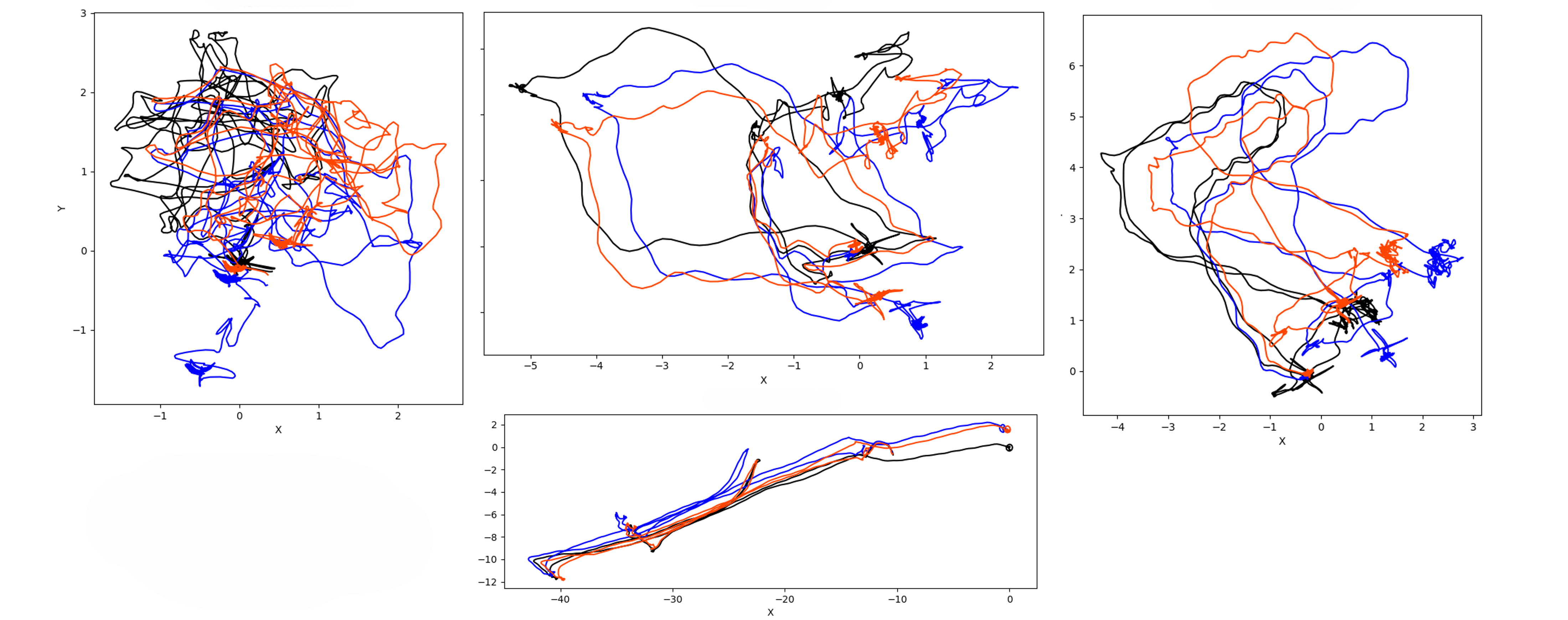
Figure 11: More Visualizations of final estimated trajectories on TLIO Dataset by baseline TLIO (Blue), our best method applied to TLIO (TLIO+Eq F. $O(2)$)(Red), and the Ground-Truth trajectory (Black).

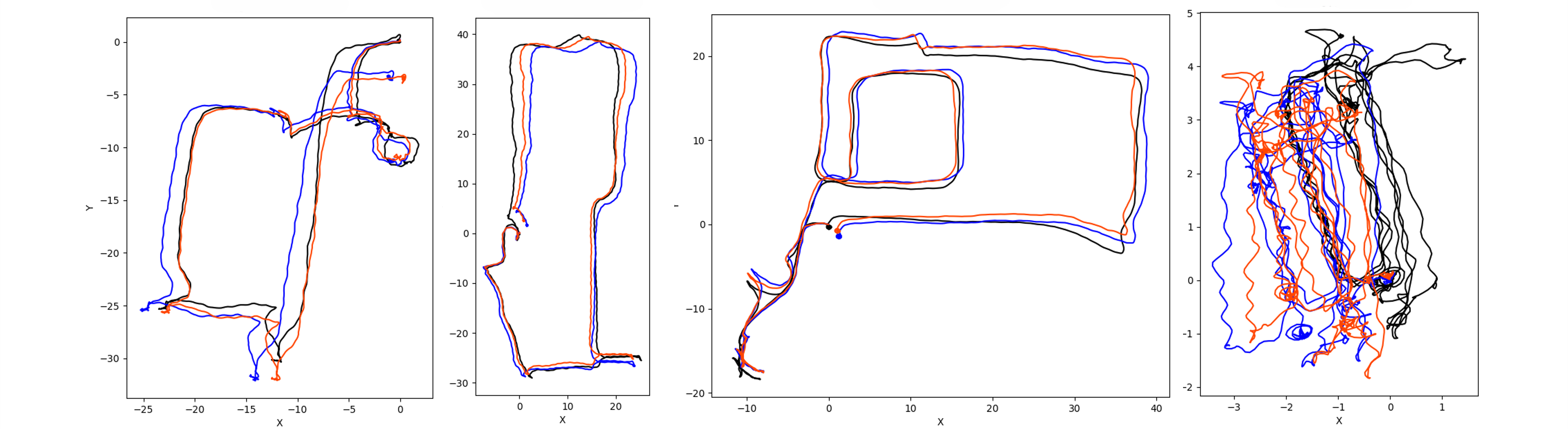
Figure 12: More Visualizations of final estimated trajectories on TLIO Dataset by baseline TLIO (Blue), our best method applied to TLIO (TLIO+Eq F. $O(2)$)(Red), and the Ground-Truth trajectory (Black).

Figure 8 and Figure 9 show only the neural network results compared to ground truth displacements. The ATE and RTE is calculated on the cumulative trajectory obtained form the predicted displacements. Figure 9 is with whisker extended to include the outlier which are commonly calculated as 1.5 * IQR (inter-quartile range). Figure 10 shows the results of EKF without excluding the outliers. We provide more trajectory visualizations of TLIO test data in Figure 11 and Figure 12.

A.7 Augmented TLIO Test Dataset Results and Analysis

We also perform an ablation study on test data augmentation for our model. For neural network results, we apply four random yaw rotations per trajectory and random rotations plus reflection per trajectory. The results are detailed in Table 4. Except for our equivariant model, all other methods show decreased performance compared to their results on non-augmented test data, whereas our model maintains consistent performance and outperforms the other methods.

For the Extended Kalman Filter (EKF) results, we augment the test data using random $SO(3)$ rotations. Notably, we do not include reflections due to the structural constraints of the Kalman filter. As shown in Table 5, despite the TLIO-NQ model outperforming ours in non-augmented tests on ATE metrics. Our model exceeds TLIO-NQ on the augmented dataset. Our approach not only sets a new benchmark but also maintains consistent performance across random rotations.

	Rotations			Rotations + Reflections
Model	MSE*	ATE*	RTE*	MSE*	ATE*	RTE*
TLIO	0.0327	3.3180	0.5417	0.0347	2.9110	0.5654
TLIO-N	0.2828	27.7797	3.1390	0.2989	23.4839	3.1313
Deeper TLIO	0.0306	3.0264	0.5300	0.0332	2.3028	0.5592
TLIO-NQ	0.0302	2.6379	0.5025	0.0331	2.3212	0.5446
TLIO-PCA	0.2286	21.3795	2.5288	0.2467	10.1660	2.2283
$\dagger$Eq F. $\mathbf{SO(2)}$	0.0319	2.3218	0.4957	0.0339	1.8664	0.5178
$\dagger$Eq F. $\mathbf{O(2)}$	0.0298	2.3305	0.4719	0.0298	1.6418	0.4361

Table 4: Ablation Study For Neural Network with Random Rotation and Reflection Transformation (4 per trajectory) on TLIO test dataset. $\dagger$ represents TLIO+. A lower error indicates a better model. The lowest values are annotated with Red. Our proposed methods are in bold.

Exp	ATE	RTE	Drift	AYE
TLIO	1.6744	0.4944	1.5526	2.7290
TLIO-N	10.3005	3.6263	2.9501	3.3684
Deeper TLIO	1.6447	0.5466	1.2767	2.7279
TLIO-NQ	1.4924	0.5119	1.2721	2.7109
TLIO-PCA	8.5787	2.9962	2.0872	3.0183
$\dagger$Eq F. $\mathbf{SO(2)}$	1.4850	0.4901	1.3029	2.7615
$\dagger$Eq F. $\mathbf{O(2)}$	1.4316	0.4592	1.3096	2.7250

Table 5: Results of evaluation of EKF with Random Rotation Transformations (4 per trajectory) on TLIO test dataset (i.e., results on augmentated test dataset). $\dagger$ represents TLIO+. A lower error indicates a better model. The lowest values are annotated with Red. Our proposed methods are in bold.

A.8 Visualization of RONIN

The visualization of trajectories in RONIN is displayed in Figure 13.

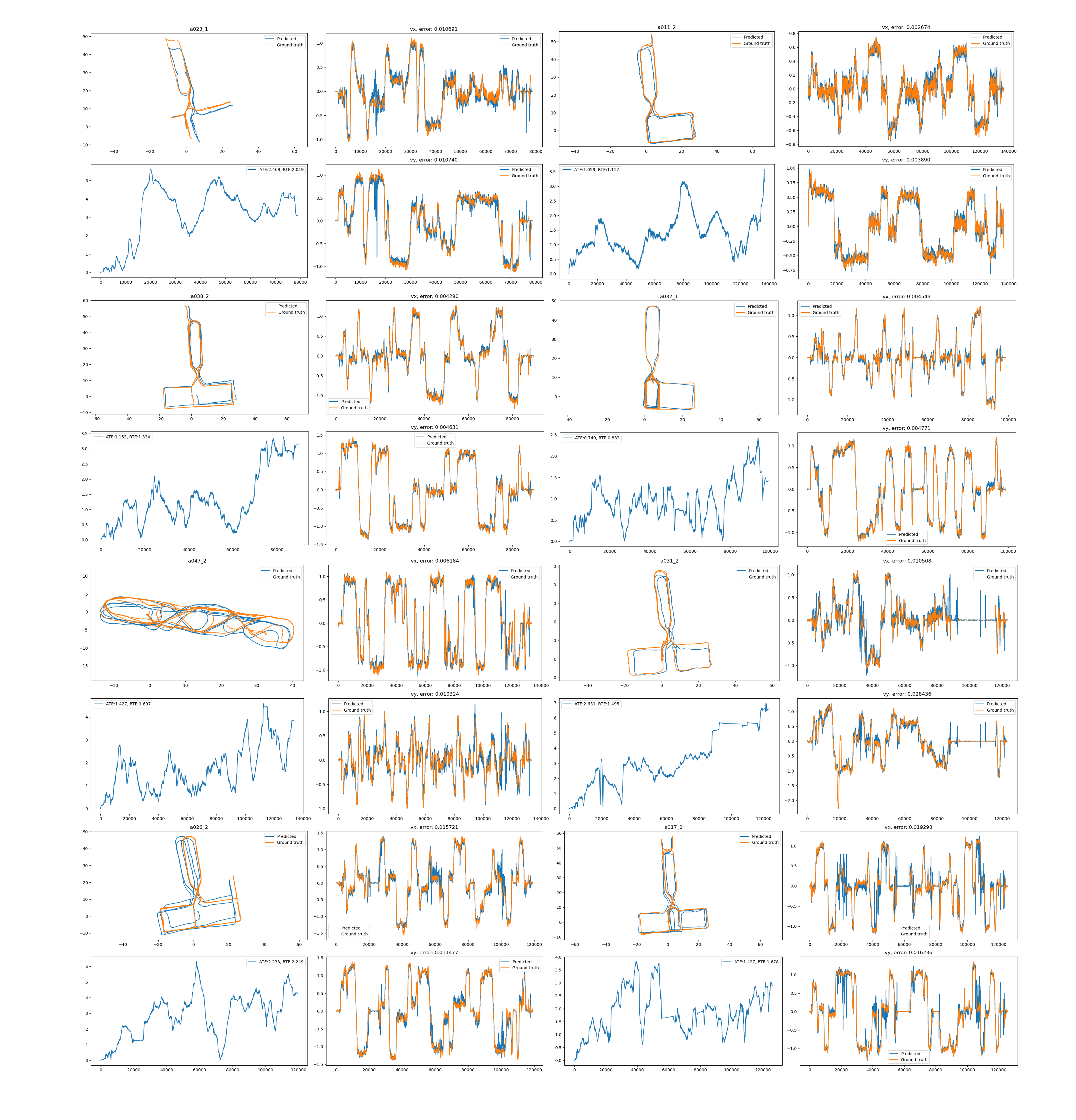
Figure 13: Visualization of RONIN Unseen Test Dataset Trajectories for our best method applied to RONIN, RONIN+Eq F. $O(2)$.

A.9 Covariance Consistency

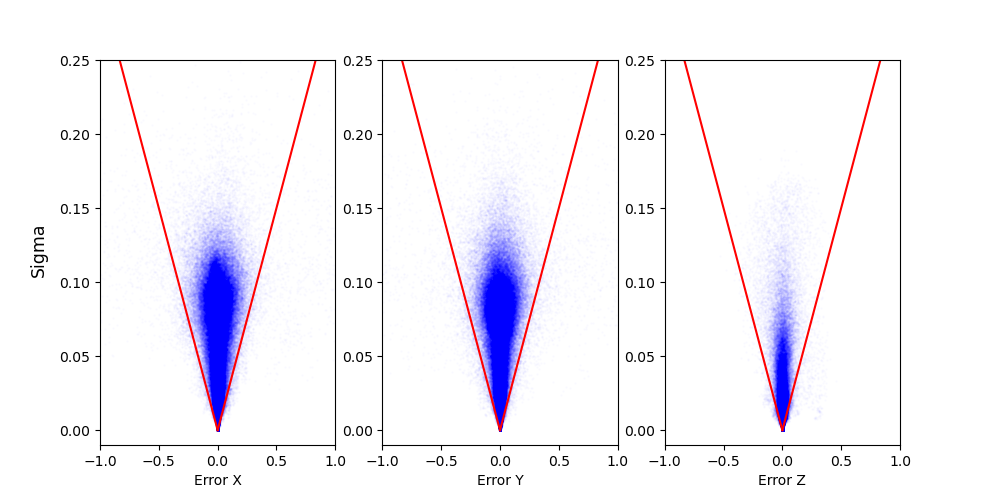
Figure 14: Consistency of Covariance Prediction in the Invariant Space for TLIO test dataset

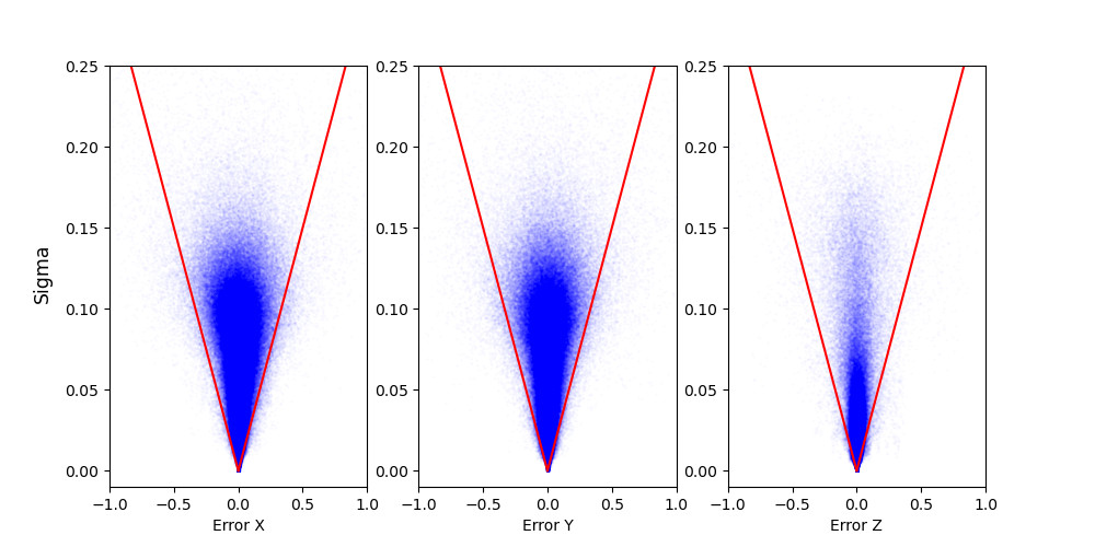
Figure 15: Consistency of Covariance Prediction in the Invariant Space for Aria dataset

Similar to TLIO [33], we plot the prediction error against standard deviation ($\sigma$) predicted by the network in the invariant space. As seen in Figure 15 and Figure 14 the covariance prediction of our method is consistently within the 3-$\sigma$ depicted by the red lines. These results show that our diagonal covariance prediction in the invariant space is consistent.

A.10 Ablation on IMU sequence length

We aligned the sequence length with baseline models for fair comparison. However, in this Section, we ablate on the sequence length as shown in Table 6 and Table 7. Table 6 varies sequence lengths and displacement prediction windows (e.g., 0.5s displacement with 0.5s of 200Hz IMU data results in a sequence length of 100). Table 7 fixes the prediction window at 1s and varies the context window (e.g., a 2s context window with 200Hz IMU data results in a sequence length of 400). Our results confirm TLIO [33] Sec. VII A.1: increasing the context window reduces MSE but not ATE. A lower MSE loss over the same displacement window does not translate to a lower ATE. Thus, the addition of the equivariant framework does not change the characteristics of the base (off-the-shelf) model used.

		TLIO Dataset			Aria Dataset
Exp	Displacement Window (s)	MSE*	ATE*	RTE*	MSE*	ATE*	RTE*
TLIO	0.5	1.132	2.029	0.340	1.038	1.489	0.332
TLIO	1	3.242	3.722	0.551	5.322	2.103	0.521
TLIO	2	9.862	5.102	0.944	6.717	3.452	0.970
$\dagger$Eq F. $SO(2)$	0.5	1.124	0.711	0.175	1.040	0.673	0.190
$\dagger$Eq F. $SO(2)$	1	3.194	2.401	0.501	2.457	1.864	0.484
$\dagger$Eq F. $SO(2)$	2	10.019	3.862	0.797	6.569	2.745	0.774
$\dagger$Eq F. $O(2)$	0.5	1.040	0.595	0.136	1.002	0.589	0.148
$\dagger$Eq F. $O(2)$	1	2.982	2.406	0.478	2.304	1.849	0.465
$\dagger$Eq F. $O(2)$	2	9.804	4.268	0.762	6.112	2.556	0.709

Table 6: Results for ablation on changing prediction displacement window on TLIO architecture. $\dagger$  represents TLIO+

		TLIO Dataset			Aria Dataset
Exp	Context Window (s)	MSE*	ATE*	RTE*	MSE*	ATE*	RTE*
TLIO	1	3.242	3.722	0.551	5.322	2.103	0.521
TLIO	2	3.199	2.555	0.511	3.790	2.895	0.713
TLIO	3	3.284	4.463	0.617	3.511	3.014	0.738
$\dagger$Eq F. $SO(2)$	1	3.194	2.401	0.501	2.457	1.864	0.484
$\dagger$Eq F. $SO(2)$	2	2.886	1.837	0.429	2.187	1.533	0.444
$\dagger$Eq F. $SO(2)$	3	2.790	3.090	0.492	1.986	1.684	0.447
$\dagger$Eq F. $O(2)$	1	2.982	2.406	0.478	2.304	1.849	0.465
$\dagger$Eq F. $O(2)$	2	2.382	1.895	0.367	1.307	1.382	0.338
$\dagger$Eq F. $O(2)$	3	2.161	2.083	0.366	0.974	1.672	0.366

Table 7: Results for ablation on changing context window with fixed displacement window of 1s on TLIO architecture. $\dagger$ represents TLIO+

A.11 Sensitivity analysis to gravity direction perturbation

		TLIO Dataset
Exp	Gravity Direction Perturbation ( in degrees)	MSE*	ATE*	RTE*
$\dagger$Eq F. $SO(2)$	0	3.194	2.401	0.501
$\dagger$Eq F. $SO(2)$	2	3.201	2.409	0.500
$\dagger$Eq F. $SO(2)$	4	3.206	2.404	0.498
$\dagger$Eq F. $SO(2)$	6	3.241	2.442	0.501
$\dagger$Eq F. $SO(2)$	8	3.298	2.502	0.506
$\dagger$Eq F. $O(2)\ddagger$	0	2.982	2.406	0.478
$\dagger$Eq F. $O(2)\ddagger$	2	3.198	2.663	0.498
$\dagger$Eq F. $O(2)\ddagger$	4	3.742	3.292	0.559
$\dagger$Eq F. $O(2)\ddagger$	6	4.505	4.228	0.659
$\dagger$Eq F. $O(2)\ddagger$	8	5.433	5.218	0.768
$\dagger$Eq F. $O(2)$	0	2.982	1.811	0.332
$\dagger$Eq F. $O(2)$	2	2.988	1.742	0.321
$\dagger$Eq F. $O(2)$	4	3.010	1.718	0.308
$\dagger$Eq F. $O(2)$	6	3.060	1.680	0.293
$\dagger$Eq F. $O(2)$	8	3.095	1.650	0.283

Table 8: Results for ablation on changing prediction displacement window on TLIO architecture. $\dagger$  represents TLIO+. $\ddagger$ implies the network was trained without gravity direction perturbation.

Similar to  Wang et al. [45], which indicates that the equivariance of $SO(2)$ can even help the rotation around another axis which is close to $z$, we believe that embedding equivariance wouldn’t harm the performance of the model when there is a slight perturbation which is inline with the experimental results as seen in Table 8.

Table 8 presents the sensitivity analysis to gravity direction perturbation, applied for 5 discrete angles. We also present results for Eq F. $O(2)$ model trained without the gravity direction perturbation of (-5°,5°) during training. We observe the same trend of stability in MSE* as reported in TLIO [33] when trained with gravity direction perturbation.

A.12 Social Impact

This work aims to utilize deep learning to mitigate drift in inertial integration for purely inertial odometry, thereby enhancing navigation efficiency and reducing costs. While our research directly contributes positively to navigation solutions and does not have inherently negative social applications, it is important to note that improved tracking and navigation capabilities could potentially be utilized for surveillance purposes, which may raise privacy concerns.

References

- Asraf et al. [2022] Omri Asraf, Firas Shama, and Itzik Klein. Pdrnet: A deep-learning pedestrian dead reckoning framework. IEEE Sensors Journal, 22(6):4932–4939, 2022. doi: 10.1109/JSEN.2021.3066840.
- Beaufils et al. [2019] Bertrand Beaufils, Frédéric Chazal, Marc Grelet, and Bertrand Michel. Robust stride detector from ankle-mounted inertial sensors for pedestrian navigation and activity recognition with machine learning approaches. Sensors, 19(20):4491, 2019.
- Bortz [1971] John E. Bortz. A new mathematical formulation for strapdown inertial navigation. IEEE Transactions on Aerospace and Electronic Systems, AES-7(1):61–66, 1971. doi: 10.1109/TAES.1971.310252.
- Brajdic and Harle [2013] Agata Brajdic and Robert Harle. Walk detection and step counting on unconstrained smartphones. In Proceedings of the 2013 ACM international joint conference on Pervasive and ubiquitous computing, pages 225–234, 2013.
- Brossard et al. [2020a] Martin Brossard, Axel Barrau, and Silvère Bonnabel. Ai-imu dead-reckoning. IEEE Transactions on Intelligent Vehicles, 5(4):585–595, 2020a. doi: 10.1109/TIV.2020.2980758.
- Brossard et al. [2020b] Martin Brossard, Silvère Bonnabel, and Axel Barrau. Denoising imu gyroscopes with deep learning for open-loop attitude estimation. IEEE Robotics and Automation Letters, 5(3):4796–4803, 2020b. doi: 10.1109/LRA.2020.3003256.
- Buchanan et al. [2023] Russell Buchanan, Varun Agrawal, Marco Camurri, Frank Dellaert, and Maurice Fallon. Deep imu bias inference for robust visual-inertial odometry with factor graphs. IEEE Robotics and Automation Letters, 8(1):41–48, 2023. doi: 10.1109/LRA.2022.3222956.
- Cao et al. [2022] Xiya Cao, Caifa Zhou, Dandan Zeng, and Yongliang Wang. Rio: Rotation-equivariance supervised learning of robust inertial odometry. In Proceedings of the IEEE/CVF Conference on Computer Vision and Pattern Recognition, pages 6614–6623, 2022.
- Cesa et al. [2021] Gabriele Cesa, Leon Lang, and Maurice Weiler. A program to build e (n)-equivariant steerable cnns. In International conference on learning representations, 2021.
- Chen et al. [2018a] Changhao Chen, Xiaoxuan Lu, Andrew Markham, and Niki Trigoni. Ionet: Learning to cure the curse of drift in inertial odometry. In Proceedings of the AAAI Conference on Artificial Intelligence, volume 32, 2018a.
- Chen et al. [2018b] Changhao Chen, Peijun Zhao, Chris Xiaoxuan Lu, Wei Wang, Andrew Markham, and Niki Trigoni. Oxiod: The dataset for deep inertial odometry. CoRR, abs/1809.07491, 2018b. URL http://arxiv.org/abs/1809.07491.
- Chen et al. [2019] Changhao Chen, Yishu Miao, Chris Xiaoxuan Lu, Linhai Xie, Phil Blunsom, Andrew Markham, and Niki Trigoni. Motiontransformer: Transferring neural inertial tracking between domains. In Proceedings of the AAAI conference on artificial intelligence, volume 33, pages 8009–8016, 2019.
- Chen et al. [2021a] Danpeng Chen, Nan Wang, Runsen Xu, Weijian Xie, Hujun Bao, and Guofeng Zhang. Rnin-vio: Robust neural inertial navigation aided visual-inertial odometry in challenging scenes. In 2021 IEEE International Symposium on Mixed and Augmented Reality (ISMAR), pages 275–283. IEEE, 2021a.
- Chen et al. [2021b] Haiwei Chen, Shichen Liu, Weikai Chen, Hao Li, and Randall Hill. Equivariant point network for 3d point cloud analysis. In Proceedings of the IEEE/CVF conference on computer vision and pattern recognition, pages 14514–14523, 2021b.
- Chen et al. [2023] Runfa Chen, Jiaqi Han, Fuchun Sun, and Wenbing Huang. Subequivariant graph reinforcement learning in 3d environments. In International Conference on Machine Learning, pages 4545–4565. PMLR, 2023.
- Cohen and Welling [2016] Taco Cohen and Max Welling. Group equivariant convolutional networks. In International conference on machine learning, pages 2990–2999. PMLR, 2016.
- Cohen et al. [2019a] Taco Cohen, Maurice Weiler, Berkay Kicanaoglu, and Max Welling. Gauge equivariant convolutional networks and the icosahedral cnn. In International conference on Machine learning, pages 1321–1330. PMLR, 2019a.
- Cohen et al. [2018] Taco S Cohen, Mario Geiger, Jonas Köhler, and Max Welling. Spherical cnns. arXiv preprint arXiv:1801.10130, 2018.
- Cohen et al. [2019b] Taco S Cohen, Mario Geiger, and Maurice Weiler. A general theory of equivariant cnns on homogeneous spaces. Advances in neural information processing systems, 32, 2019b.
- Deng et al. [2021] Congyue Deng, Or Litany, Yueqi Duan, Adrien Poulenard, Andrea Tagliasacchi, and Leonidas J Guibas. Vector neurons: A general framework for so (3)-equivariant networks. In Proceedings of the IEEE/CVF International Conference on Computer Vision, pages 12200–12209, 2021.
- Esteves et al. [2018] Carlos Esteves, Christine Allen-Blanchette, Ameesh Makadia, and Kostas Daniilidis. Learning so (3) equivariant representations with spherical cnns. In Proceedings of the European Conference on Computer Vision (ECCV), pages 52–68, 2018.
- Esteves et al. [2019] Carlos Esteves, Yinshuang Xu, Christine Allen-Blanchette, and Kostas Daniilidis. Equivariant multi-view networks. In Proceedings of the IEEE/CVF international conference on computer vision, pages 1568–1577, 2019.
- Esteves et al. [2020] Carlos Esteves, Ameesh Makadia, and Kostas Daniilidis. Spin-weighted spherical cnns. Advances in Neural Information Processing Systems, 33:8614–8625, 2020.
- Esteves et al. [2023] Carlos Esteves, Jean-Jacques Slotine, and Ameesh Makadia. Scaling spherical cnns. arXiv preprint arXiv:2306.05420, 2023.
- Finzi et al. [2021] Marc Finzi, Max Welling, and Andrew Gordon Wilson. A practical method for constructing equivariant multilayer perceptrons for arbitrary matrix groups. In International conference on machine learning, pages 3318–3328. PMLR, 2021.
- Foxlin [2005] Eric Foxlin. Pedestrian tracking with shoe-mounted inertial sensors. IEEE Computer graphics and applications, 25(6):38–46, 2005.
- Groves [2015] Paul D Groves. Principles of gnss, inertial, and multisensor integrated navigation systems, [book review]. IEEE Aerospace and Electronic Systems Magazine, 30(2):26–27, 2015.
- Han et al. [2022] Jiaqi Han, Wenbing Huang, Hengbo Ma, Jiachen Li, Josh Tenenbaum, and Chuang Gan. Learning physical dynamics with subequivariant graph neural networks. Advances in Neural Information Processing Systems, 35:26256–26268, 2022.
- Hartley et al. [2020] Ross Hartley, Maani Ghaffari, Ryan M Eustice, and Jessy W Grizzle. Contact-aided invariant extended kalman filtering for robot state estimation. The International Journal of Robotics Research, 39(4):402–430, 2020.
- Herath et al. [2020] Sachini Herath, Hang Yan, and Yasutaka Furukawa. Ronin: Robust neural inertial navigation in the wild: Benchmark, evaluations, and new methods. In IEEE International Conference on Robotics and Automation (ICRA), pages 3146–3152. IEEE, 2020.
- Ho et al. [2016] Ngoc-Huynh Ho, Phuc Huu Truong, and Gu-Min Jeong. Step-detection and adaptive step-length estimation for pedestrian dead-reckoning at various walking speeds using a smartphone. Sensors, 16(9):1423, 2016.
- Jimenez et al. [2009] Antonio R Jimenez, Fernando Seco, Carlos Prieto, and Jorge Guevara. A comparison of pedestrian dead-reckoning algorithms using a low-cost mems imu. In 2009 IEEE International Symposium on Intelligent Signal Processing, pages 37–42. IEEE, 2009.
- Liu et al. [2020] Wenxin Liu, David Caruso, Eddy Ilg, Jing Dong, Anastasios I Mourikis, Kostas Daniilidis, Vijay Kumar, and Jakob Engel. Tlio: Tight learned inertial odometry. IEEE Robotics and Automation Letters, 5(4):5653–5660, 2020.
- Lv et al. [2024] Zhaoyang Lv, Nickolas Charron, Pierre Moulon, Alexander Gamino, Cheng Peng, Chris Sweeney, Edward Miller, Huixuan Tang, Jeff Meissner, Jing Dong, et al. Aria everyday activities dataset. arXiv preprint arXiv:2402.13349, 2024.
- Rajagopal [2008] Sujatha Rajagopal. Personal dead reckoning system with shoe mounted inertial sensors. Master’s Degree Project, Stockholm, Sweden, 2008.
- Russell and Reale [2021] Rebecca L Russell and Christopher Reale. Multivariate uncertainty in deep learning. IEEE Transactions on Neural Networks and Learning Systems, 33(12):7937–7943, 2021.
- Satorras et al. [2021] Vıctor Garcia Satorras, Emiel Hoogeboom, and Max Welling. E (n) equivariant graph neural networks. In International conference on machine learning, pages 9323–9332. PMLR, 2021.
- Solin et al. [2018] Arno Solin, Santiago Cortes, Esa Rahtu, and Juho Kannala. Inertial odometry on handheld smartphones. In 2018 21st International Conference on Information Fusion (FUSION), pages 1–5. IEEE, 2018.
- Steinbrener et al. [2022] Jan Steinbrener, Christian Brommer, Thomas Jantos, Alessandro Fornasier, and Stephan Weiss. Improved state propagation through ai-based pre-processing and down-sampling of high-speed inertial data. In 2022 International Conference on Robotics and Automation (ICRA), pages 6084–6090, 2022. doi: 10.1109/ICRA46639.2022.9811989.
- Sun et al. [2021] Scott Sun, Dennis Melamed, and Kris Kitani. Idol: Inertial deep orientation-estimation and localization. In Proceedings of the AAAI Conference on Artificial Intelligence, volume 35, pages 6128–6137, 2021.
- Thomas et al. [2018] Nathaniel Thomas, Tess Smidt, Steven Kearnes, Lusann Yang, Li Li, Kai Kohlhoff, and Patrick Riley. Tensor field networks: Rotation-and translation-equivariant neural networks for 3d point clouds. arXiv preprint arXiv:1802.08219, 2018.
- Titterton et al. [2004] D. Titterton, J.L. Weston, Institution of Electrical Engineers, American Institute of Aeronautics, and Astronautics. Strapdown Inertial Navigation Technology. IEE Radar Series. Institution of Engineering and Technology, 2004. ISBN 9780863413582. URL https://books.google.com/books?id=WwrCrn54n5cC.
- Umeyama [1991] S. Umeyama. Least-squares estimation of transformation parameters between two point patterns. IEEE Transactions on Pattern Analysis and Machine Intelligence, 13(4):376–380, 1991. doi: 10.1109/34.88573.
- Villar et al. [2021] Soledad Villar, David W Hogg, Kate Storey-Fisher, Weichi Yao, and Ben Blum-Smith. Scalars are universal: Equivariant machine learning, structured like classical physics. Advances in Neural Information Processing Systems, 34:28848–28863, 2021.
- Wang et al. [2023] Dian Wang, Jung Yeon Park, Neel Sortur, Lawson L. S. Wong, Robin Walters, and Robert Platt. The surprising effectiveness of equivariant models in domains with latent symmetry, 2023. URL https://arxiv.org/abs/2211.09231.
- Weiler and Cesa [2019] Maurice Weiler and Gabriele Cesa. General e (2)-equivariant steerable cnns. Advances in neural information processing systems, 32, 2019.
- Weiler et al. [2018] Maurice Weiler, Mario Geiger, Max Welling, Wouter Boomsma, and Taco S Cohen. 3d steerable cnns: Learning rotationally equivariant features in volumetric data. Advances in Neural Information Processing Systems, 31, 2018.
- Weiler et al. [2021] Maurice Weiler, Patrick Forré, Erik Verlinde, and Max Welling. Coordinate independent convolutional networks–isometry and gauge equivariant convolutions on riemannian manifolds. arXiv preprint arXiv:2106.06020, 2021.
- Worrall et al. [2017] Daniel E Worrall, Stephan J Garbin, Daniyar Turmukhambetov, and Gabriel J Brostow. Harmonic networks: Deep translation and rotation equivariance. In Proceedings of the IEEE conference on computer vision and pattern recognition, pages 5028–5037, 2017.
- Xu et al. [2022] Yinshuang Xu, Jiahui Lei, Edgar Dobriban, and Kostas Daniilidis. Unified fourier-based kernel and nonlinearity design for equivariant networks on homogeneous spaces. In International Conference on Machine Learning, pages 24596–24614. PMLR, 2022.
- Xu et al. [2024] Yinshuang Xu, Jiahui Lei, and Kostas Daniilidis. equivariant convolution and transformer in ray space. Advances in Neural Information Processing Systems, 36, 2024.
- Yan et al. [2018] Hang Yan, Qi Shan, and Yasutaka Furukawa. Ridi: Robust imu double integration. In Proceedings of the European Conference on Computer Vision (ECCV), September 2018.