Superuniversal Statistics of Complex Time-Delays in Non-Hermitian Scattering Systems

Abstract

The Wigner-Smith time-delay of flux conserving systems is a real quantity that measures how long an excitation resides in an interaction region. The complex generalization of time-delay to non-Hermitian systems is still under development, in particular, its statistical properties in the short-wavelength limit of complex chaotic scattering systems has not been investigated. From the experimentally measured multi-port scattering ($S$)-matrices of one-dimensional graphs, a two-dimensional billiard, and a three-dimensional cavity, we calculate the complex Wigner-Smith ($\tau_{WS}$), as well as each individual reflection ($\tau_{xx}$) and transmission ($\tau_{xy}$) time-delays. The complex reflection time-delay differences ($\tau_{\delta R}$) between each port are calculated, and the transmission time-delay differences ($\tau_{\delta T}$) are introduced for systems exhibiting non-reciprocal scattering. Large time-delays are associated with coherent perfect absorption, reflectionless scattering, slow light, and uni-directional invisibility. We demonstrate that the large-delay tails of the distributions of the real and imaginary parts of each of these time-delay quantities are superuniversal, independent of experimental parameters: uniform attenuation $\eta$, number of scattering channels $M$, wave propagation dimension $\mathcal{D}$, and Dyson symmetry class $\beta$. This superuniversality is in direct contrast with the well-established time-delay statistics of unitary scattering systems, where the tail of the $\tau_{WS}$ distribution depends explicitly on the values of $M$ and $\beta$. Due to the direct analogy of the wave equations, the time-delay statistics described in this paper are applicable to any non-Hermitian wave-chaotic scattering system in the short-wavelength limit, such as quantum graphs, electromagnetic, optical and acoustic resonators, etc.

Introduction.—In this Letter, we consider the wave-scattering properties of complex systems with a finite number of asymptotic scattering channels coupled to the outside world. The systems of interest have dimensions much larger than the wavelength of the waves, making the scattering properties extremely sensitive to details, such as boundary shapes and interior scattering centers. Such systems could be three-dimensional spaces such as rooms, two-dimensional billiards, or one-dimensional graphs, and the waves could be electromagnetic, acoustic, or quantum in nature. The complexity of wave propagation and interference is captured by the scattering $S$-matrix which transforms a vector of input excitations $\ket{\psi_{\text{in}}}$ on $M$ channels to a vector of outputs $\ket{\psi_{\text{out}}}$ as $\ket{\psi_{\text{out}}}=S\ket{\psi_{\text{in}}}$. The scattering diversity gives rise to strong dependence of the complex $S$-matrix elements as a function of excitation energy $E$. We focus in particular on the time these waves spend in the scattering region as they propagate from one scattering channel to another. An average dwell-time was introduced by Wigner [1] in the context of nuclear scattering. Smith [2] later generalized this idea by inventing a lifetime matrix $Q=i\hbar S\frac{dS^{\dagger}}{dE}$, the normalized trace of which is defined as the Wigner-Smith time-delay $\tilde{\tau}_{WS}=\frac{1}{M}\text{Tr}[Q]$, which is strictly real for unitary (flux-conserving) systems.

For a quantum mechanical wave, $\tilde{\tau}_{WS}$ can be directly related to the phase evolution of a wave packet and its group delay [3, 4]. For classical waves, the Wigner-Smith time-delay is simply the energy dependent shift in arrival time caused by the scattering interaction [5]. Some examples of the physical uses of time-delay are in nuclear physics [6, 7], group delay of modes in waveguides and optical fibers [8, 9, 10, 11, 12], wavefront shaping and creation of particlelike scattering states [13, 14, 15, 16, 17], radio frequency pulse propagation [18, 19], radiation intensity statistics [20, 21], identifying zeros and poles of the scattering matrix [22, 23, 24, 25, 26, 27], characterization of disordered and biological media [28, 29, 30, 31, 32, 33], and in acoustics [34].

When studying scattering of short-wavelength excitations in complex systems, such as nuclei or irregular electromagnetic structures, it is appropriate to examine the statistical properties of time-delays, due to the sensitive energy and parametric variations of the scattering process. Random Matrix Theory (RMT) has been very successful at describing universal fluctuations of time-delays in unitary scattering systems [35, 36, 37, 22, 38, 39, 40, 41, 42, 43, 44, 45, 46, 47, 48]. This body of work discovered that the probability distribution $\mathcal{P}(\tilde{\tau}_{WS})$ has certain consistent properties. One of particular interest is the shape of $\mathcal{P}(\tilde{\tau}_{WS})$ at extreme values, which correspond to modes with long scattering times. It was found independently by several groups that the distribution of the Wigner-Smith time-delay of a perfectly coupled system has an algebraic power-law decay for large values of the time-delay described by $\mathcal{P}(\tilde{\tau}_{WS})\propto\tilde{\tau}_{WS}^{-(M\beta)/2-2}$ [49, 50, 51, 52, 53, 54, 55, 56] where $\beta$ is the Dyson symmetry class of the system [57]. A more complete review of Wigner-Smith time-delay results and analysis in unitary scattering systems can be found in Ref. [58].

Physically realizable systems invariably have loss and/or gain, and this non-Hermiticity cannot be ignored when examining experimental scattering data [59, 60, 61, 62, 63, 64, 65, 66, 67, 68, 31]. For weak attenuation, an expansion about the unitary scattering matrix is possible [69, 70, 71, 72], but the most general way to account for dissipation leads to a complex $\tilde{\tau}_{WS}$ [5, 73, 17, 26]. We also consider the time-delays associated with each element of the $S$-matrix. Even when the scattering matrix is unitary, the reflection and transmission submatrices are subunitary, leading to complex time-delays describing reflection and transmission processes [5, 74]. The reflection time-delay difference between channels has been proposed as a quantity that depends only on the reflection zeros of the system, and to be independent of the poles of the scattering matrix [27, 25, 24]. Finally, we introduce the complex transmission time-delay difference in non-reciprocal scattering systems which depends solely on the system’s transmission zeros.

The presence of absorption introduces qualitatively new phenomena not seen in unitary systems, such as Coherent Perfect Absorption (CPA), in which all the energy injected into a system is completely absorbed, with no reflection or transmission on any of the scattering channels [75, 23, 76, 77, 16, 17, 78, 79]. CPA has been associated with diverging Wigner-Smith time-delays [17, 80], justifying attention to the large value tail of the distribution. Similarly, divergences of the reflection time-delay correspond to reflectionless scattering modes (RSM) [81, 82, 79], divergence of the transmission time-delay indicates the system could be used as a “slow-light” medium [83, 84, 85], while the divergence of the transmission time-delay difference could identify points of uni-directional invisibility [86, 87, 88].

Recently, Chen, et al. showed that $\mathcal{P}(\tilde{\tau}_{WS})$ of the complex quantity for a perfectly coupled $M=2$ channel, non-reciprocal ($\beta=2$) system with finite uniform absorption strength $\eta$ has $-3$ power-law tails. They predicted that this should be true for all perfectly coupled non-Hermitian systems independent of all other parameters [89]. This is in contrast with the tail of the time-delay distribution in the unitary case which depends explicitly on both $M$ and $\beta$. In this Letter, we examine the statistics of each complex time-delay (CTD) quantity with a focus on the asymptotic behavior of their distributions. We examine four parameters which could dictate the distribution tails: (i) dimension for wave propagation $\mathcal{D}$, (ii) number of scattering channels $M$, (iii) Dyson symmetry class $\beta$, and (iv) uniform absorption strength $\eta$.

We first provide the theory and definitions of CTD in non-Hermitian systems, then present the systems experimentally investigated, and finally we discuss the superuniversal $-3$ power-law heavy-tail of the CTD probability distributions. This result shows that the probability of finding singularities such as CPA, RSM, and transparency in arbitrary scattering systems with controlled perturbations, such as through the use of metamaterials [78, 90, 16, 91, 92, 93, 79], is quite high. Such perturbations can be accomplished not only with microwaves, but also in acoustics [94, 95, 96] and optics [97, 98, 99].

Theory.—In the Heidelberg approach to wave scattering [100, 101, 22, 102, 103, 104], the non-Hermitian effective Hamiltonian of a scattering environment $\mathcal{H}_{\text{eff}}=H-i\Gamma_{W}$ is constructed from the $N\crossproduct N$ Hamiltonian $H$ describing the closed system and the $N\crossproduct M$ matrix $W$ of coupling coefficients between the $N$ modes of $H$ and the $M$ scattering channels, where $\Gamma_{W}=\pi WW^{\dagger}$. The energy-dependent scattering matrix $S(E)$ takes the form [101, 22, 103]

$$S(E)=1_{M\crossproduct M}-2\pi iW^{\dagger}\frac{1}{E-\mathcal{H}_{\text{eff}}}W=\begin{pmatrix}S_{11}&\dots&S_{1M}\\ \vdots&\ddots&\vdots\\ S_{M1}&\dots&S_{MM}\end{pmatrix}.$$

One can account for a spatially uniform attenuation of the waves with rate $\tilde{\eta}$ by making the substitution $E\rightarrow E+i\tilde{\eta}$ and evaluating the resulting subunitary $S$-matrix at complex energies. Experimentally, such a subunitary scattering matrix for an $M$-channel system is measured as $S(E)$ in terms of $M^{2}$ energy-dependent complex reflection ($S_{xx}$) and transmission ($S_{xy}$) submatrices where $x\neq y$ and $x,y\in[1,\dots,M]$ [105, 80, 106, 107]. Describing uniform loss in this manner is phenomenological and makes no special assumptions about the $S$-matrix, so it applies generally to all classical wave scattering systems. Therefore although all the results discussed in this paper are for electromagnetic waves, the conclusions should hold for other waves in non-Hermitian scattering systems.

The Wigner-Smith time-delay extended to non-Hermitian systems has a natural definition as a complex quantity [26]:

$$\tilde{\tau}_{WS}:=\frac{-i}{M}\frac{\partial}{\partial E}\text{log}[\text{det}S(E+i\tilde{\eta})].$$ (1)

$\tilde{\tau}_{WS}$ can also be written as a sum of Lorentzian functions of energy in terms of the $S$-matrix poles ($\mathcal{E}_{n}=E_{n}-i\Gamma_{n}$) and zeros ($z_{n}$), which are the complex eigenvalues of $\mathcal{H}_{\text{eff}}$ and $\mathcal{H}_{\text{eff}}^{\dagger}$ respectively [26, 108]. Complex $\tilde{\tau}_{WS}$ is therefore a useful quantity for extracting the complex poles and zeros of the scattering matrix [27].

While $\tilde{\tau}_{WS}$ takes into account the entire scattering matrix, sometimes it is useful to consider the time-delays of individual reflection and transmission processes [109, 110, 5, 73, 74, 111, 112, 113]. The CTDs for reflection at channel $x$ and transmission to channel $x$ from channel $y$ are given by [27]

$$\tilde{\tau}_{xx}:=-i\frac{\partial}{\partial E}\text{log}[S_{xx}]$$ (2a)

$$\tilde{\tau}_{xy}:=-i\frac{\partial}{\partial E}\text{log}[S_{xy}]$$ (2b)

in direct analogy with $\tilde{\tau}_{WS}$. These time-delays can also be written as sums of Lorentzian functions of energy which depend on the $S$-matrix poles ($\mathcal{E}_{n}$) and the individual reflection ($r_{n}$) and transmission ($t_{n}$) zeros [114, 27].

Since the Lorentzian terms arising from the poles are identical for each reflection and transmission time-delay, we can define new quantities, the reflection and transmission time-delay differences, which are expected to be independent of the S-matrix poles [27, 25, 24]:

$$\tilde{\tau}_{\delta R}:=\tilde{\tau}_{xx}-\tilde{\tau}_{yy}=-i\frac{\partial}{\partial E}\text{log}[\frac{S_{xx}}{S_{yy}}]$$ (3a)

$$\tilde{\tau}_{\delta T}:=\tilde{\tau}_{xy}-\tilde{\tau}_{yx}=-i\frac{\partial}{\partial E}\text{log}[\frac{S_{xy}}{S_{yx}}].$$ (3b)

It is very common to have $S_{xx}\neq S_{yy}$ so $\tilde{\tau}_{\delta R}$ of an arbitrary system is almost always non-zero. In contrast, to have a non-trivial $\tilde{\tau}_{\delta T}$ the system must have non-reciprocal transmission, and this can be accomplished, for example, with electromagnetic waves propagating through magnetized ferrite materials, [115, 116, 117, 118, 119, 120, 121, 122, 123, 124]. The transmission time-delay difference written as sums of Lorenztian functions of energy is given for the first time in Eqs. S1-S2.

In highly over-moded structures, CTDs vary wildly as a function of energy (or equivalently frequency $f$), with both the real and imaginary parts taking on positive and negative values [5, 26, 17, 27] (see Fig. S3(a) for a representative example). Since CTD is very sensitive to perturbations of an over-moded scattering system, we don’t focus on the time-delay of any specific system, but instead examine the distribution of time-delays from a statistical ensemble of many similar systems.

Experiment.—Microwave experiments have proven to be ideal platforms for investigating fluctuations in wave scattering properties of complex systems [125, 126, 127, 128, 129, 103, 130, 131]. The experimental data presented in this paper comes from $M\times M$ scattering matrices $S$ collected through the use of calibrated Keysight PNA-X N5242A and PNA-X N5242B microwave vector network analyzers. The measured scattering parameters from the PNA contain information about the coupling of the system being measured to the outside world, as well as direct processes (which include short orbits between ports). These non-universal effects are removed through application of the random coupling model (RCM) normalization process, which results in an $S$-matrix with perfect coupling, and reduces the effects of short orbits on the statistics [132, 62, 63, 64, 133, 134, 135, 136, 137, 68, 130, 138, 139].

Because physical systems have system-specific shape and size, the value in seconds of any time-delay $\tilde{\tau}$ is dependent to some extent on irrelevant details. To isolate the universally-fluctuating properties, it is necessary to normalize $\tilde{\tau}$ by the Heisenberg time $\tau_{H}=\frac{2\pi}{\Delta}$ where $\Delta$ is the mean mode spacing of the closed system [89, 140, 141]. The scaled time-delays $\tau:=\tilde{\tau}/\tau_{H}$ discussed in this Letter are dimensionless quantities independent of the specific system measured. We also normalize the absorption rate of the system to a dimensionless quantity in units of the Heisenberg time $\eta:=\tau_{H}\tilde{\eta}$.

Our $\mathcal{D}=1$ system is an irregular tetrahedral graph with phase shifters on the bonds [142, 139, 143, 144, 145], depicted schematically in Fig. 1, which is a well-studied graph topology [146, 147, 75, 148, 76, 149, 150, 151, 152]. For $\mathcal{D}=2$ and $\mathcal{D}=3$ we used a two-dimensional ray-chaotic 1/4-bow-tie billiard [126, 116, 153, 154, 131] and a three-dimensional ray-chaotic cavity [155, 156, 157, 158, 159, 160, 16, 91], each containing voltage controlled metasurfaces [90, 92, 91, 93, 78]. A schematic of the billiard used in the experiment is shown in Fig. 1 of Ref. [78], and a photograph of the cavity and metasurface is given in Fig. S2. We measured these systems with $M=1,2,3$ scattering channels. The Dyson symmetry class $\beta$ of a system can be changed from $1$ to $2$ through inclusion of a magnetized ferrite in the microwave propagation path, such as including a circulator at one of the nodes in a graph [161, 162, 120, 121, 122, 163, 164]. We also consider a graph that has a circulator on every node connected to a scattering channel, but nowhere else, which we term “non-reciprocal coupling” (NRC), as a special case of $\beta=2$. An explicit diagram of an NRC graph is shown in Fig. S1. Each system has its own intrinsic uniform absorption strength $\eta$ which is frequency dependent [27], so by measuring in different frequency bands we can systematically vary the value of $\eta$. The uniform attenuation can also be increased by uniformly distributing absorbers in a cavity [132, 165, 65, 67] or attenuators on the bonds of a graph. The absorption rate of the systems considered here varied from $\eta=1.76$ to $\eta=49.01$, creating data in the low, moderate, and high absorption strength regimes [166, 147, 132, 59, 60, 167, 123].

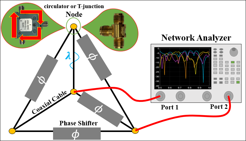
Figure 1: Schematic of an experimentally realized irregular $M=2$ tetrahedral graph. Four of the six bonds of the graph are comprised of phase shifters. Each node can be an SMA T-adapter/junction or microwave circulator.

More details on the specific experimental systems as well as the creation of statistical ensembles can be found in Supp. Mat. Sec. S1.

Discussion.—We present the probability distribution functions (PDFs) of the CTDs calculated using Eqs (1-3b) from the measured ensembles of $S$-matrix data that have been RCM-normalized to establish perfect coupling at all frequencies.

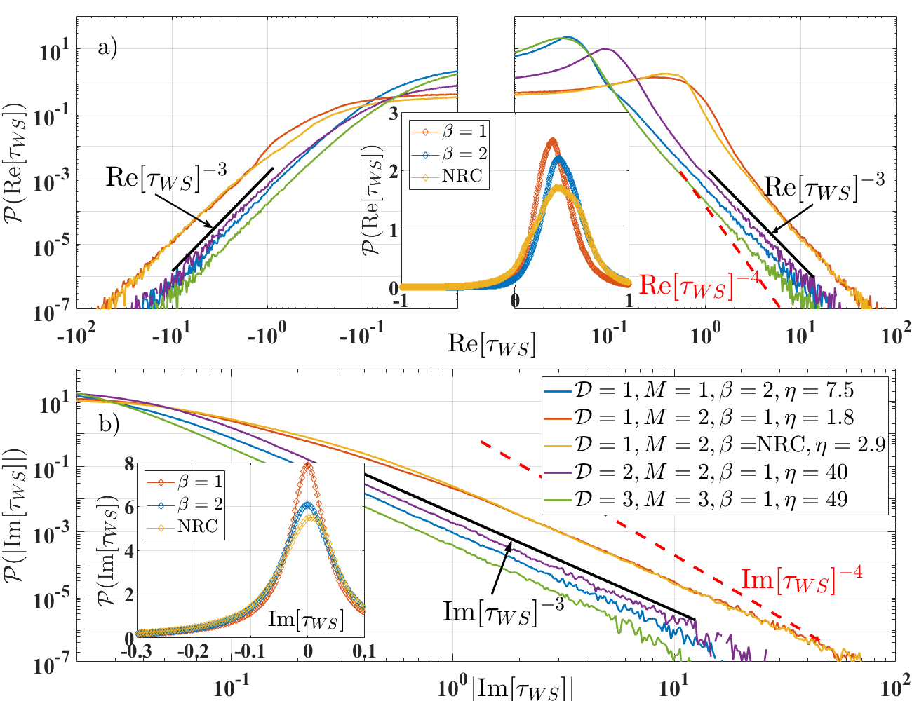
Figure 2: PDFs of (a) Re$[\tau_{WS}]$ and (b) $\lvert$Im$[\tau_{WS}]$$\rvert$ Wigner-Smith CTD from ensembles of experimental scattering systems with different values for the four parameters $\mathcal{D},M,\beta,\eta$. Black reference line characterizes asymptotic behavior as $\tau_{WS}^{-3}$ power-law for all distributions. Dashed red line depicts $-4$ power-law showing deviation from distributions. Insets depict representative distributions of a $\beta=1,\beta=2$ and NRC system on a linear scale, all with $\mathcal{D}=1,M=2$ and approximately equal $\eta$.

Figure 2(a) shows the distributions of Re$[\tau_{WS}]$ for five systems with different values for the four experimental parameters, $\mathcal{D},M,\beta,\eta$, and Fig. 2(b) shows the PDFs of $|$Im$[\tau_{WS}]|$. The black lines are not fits, but $-3$ power-laws placed nearby to characterize the large-delay tail behavior. For large values of $\tau_{WS}$, all of the distributions have parallel tails with the same slope as the black reference line. If the non-Hermitian time-delay distributions followed the Hermitian prediction, we would expect to see in Fig. 2 three different power-law tails of slope: $-3,-3.5,-4$. The dashed red line in Fig. 2 depicts a $-4$ power-law, which clearly deviates from the tail behavior of the distributions.

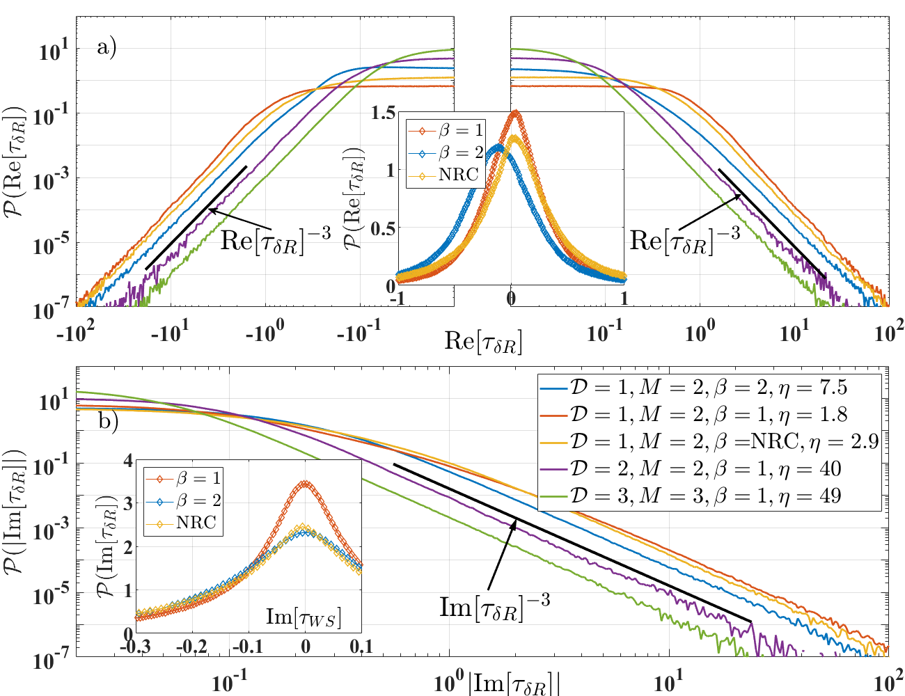
Figure 3: PDFs of (a) Re$[\tau_{\delta R}]$ and (b) $\lvert$Im$[\tau_{\delta R}]$$\rvert$ reflection time-delay difference from ensembles of experimental scattering systems with different values for the four parameters $\mathcal{D},M,\beta,\eta$. Insets and reference lines serve the same purpose as in Fig. 2.

Individual complex reflection and transmission time-delay distributions calculated from Eqs. 2a-2b are presented in Supplemental Material Sec. S3. The tails of these distributions, both real and imaginary, are also $-3$ power-law tails.

We also look at the distributions of the CTD differences, as defined in Eqs. 3a-3b. Fig. 3 shows $\mathcal{P}(\tau_{\delta R})$ of five systems with varying parameters. An $M$ channel system has $\frac{M(M-1)}{2}$ reflection time-delay differences. For the $M=3$ systems measured in the experiment it was found that the distributions of each pairwise difference have identical tails with only slight differences in the shape of the PDF at small values of $\tau_{\delta R}$. For that reason we only present the distribution of one difference for the $M=3$ system in Fig. 3, which is the green line.

In Figs. 2-3, S4-S5 the $-3$ power-law tails of distributions from large-$\eta$ systems onset at smaller values of the respective CTD. This suggest that the $-3$ power-law is indeed associated with finite loss, distinguishing non-Hermitian systems from flux-preserving ones. Note that prior work has characterized the mean of $\mathcal{P}(\text{Re}[\tau_{WS}])$ as a function of $\eta$ [89].

Fig. 4 shows the distributions of $\tau_{\delta T}$ for six systems with $\mathcal{D}=1$ and $\beta=2$, two of which have non-reciprocal coupling (NRC). For this work all measured broken-reciprocity systems were graphs.

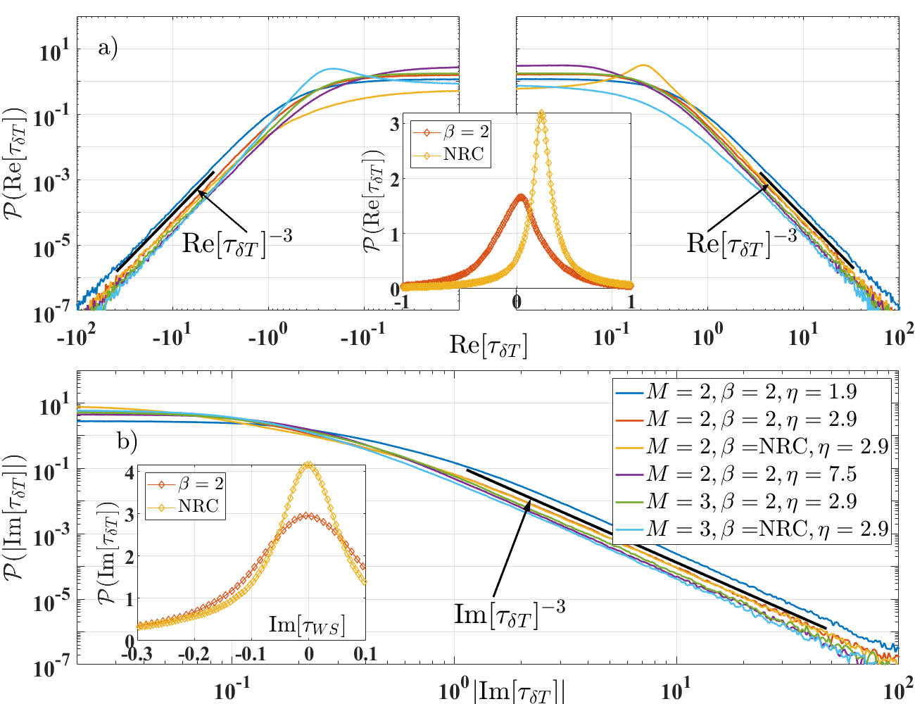
Figure 4: PDFs of (a) Re$[\tau_{\delta T}]$ and (b) $\lvert$Im$[\tau_{\delta T}]$$\rvert$ transmission time-delay difference from ensembles of experimental scattering systems with different values for $M$ and $\eta$, and two different non-reciprocal graphs. All distributions come from graphs ($\mathcal{D}=1$). Insets and reference lines serve the same purpose as in Fig. 2.

There are $\frac{{M\choose 2}\left({M\choose 2}-1\right)}{2}$ unique transmission time-delay differences that one can define, of five different types: (1) between the same two ports (e.g. $\tau_{12}-\tau_{21}$) as in Eq. 3b, (2) transmission to the same port (e.g. $\tau_{12}-\tau_{13}$), (3) transmission from the same port (e.g. $\tau_{21}-\tau_{31}$), (4) a travelling transmission (e.g. $\tau_{21}-\tau_{32}$), (5) and transmission across completely different ports (e.g. $\tau_{21}-\tau_{43}$). In Fig. 4 we show only the first kind of transmission time-delay difference, but types (1-4) all have the same $-3$ power-law tails. It should be noted that types (2-4) show $-3$ power-law tails even for reciprocal systems. The fifth kind of transmission difference requires $M\geq 4$, which we did not experimentally measure for this study.

Across Figs. 2-4 and Figs. S4-S5 we show empirical evidence for a superuniversal $-3$ power-law tail behavior for every CTD ($\tau_{WS},\tau_{xx},\tau_{xy},\tau_{\delta R},\tau_{\delta T}$) distribution of perfectly coupled non-Hermitian systems. This power-law is completely independent of system dimension $\mathcal{D}$, number of scattering channels $M$, Dyson symmetry class $\beta$, and absorption strength $\eta$. The heavy-tail on all these distributions implies that there is an abundance of long-time events (such as CPAs, RSMs, etc.) in arbitrary non-Hermitian scattering systems, and that no CTD quantity has a finite variance. Compare this to the established variance of the real $\tau_{WS}$ of Hermitian systems which has a diverging variance only for $M\beta=2$ [44, 168, 55].

In Supplemental Material Sec. S4 we demonstrate that the $-3$ power-law tail is also displayed in the distributions of CTD calculated from RMT numerical data, using the same set of parameters we used in the experiment. By comparing experiment and RMT numerics, it is evident that the behavior of the experimental distributions at small values of time-delay are clearly non-trivial and system dependent [111, 89], in contrast to the long-time tails. The statistics of time-delays derived from $S$-matrix data taken from systems with imperfect and frequency dependent coupling are shown in Supplemental Materials Section S5.2.

Concerning theory, it can be shown through resonance representation that $\mathcal{P}(\tau_{WS})$ of a perfectly coupled system is expected to have various regimes described by different algebraic forms [89]. For extreme values of $\text{Re}[\tau_{WS}]$ and $\text{Im}[\tau_{WS}]$, it is predicted that $\mathcal{P}(\text{Re}[\tau_{WS}])\propto\text{Re}[\tau_{WS}]^{-3}$ and $\mathcal{P}(\text{Im}[\tau_{WS}])\propto\text{Im}[\tau_{WS}]^{-3}$ for arbitrary systems, independent of all parameters. This asymptotic power-law tail is exactly that seen for all systems examined here (Fig. 2). Separately, it was also predicted that the distribution of the real component of the reflection time-delay difference also has a tail with an algebraic decay described by $\mathcal{P}(\text{Re}[\tau_{\delta R}])\propto\text{Re}[\tau_{\delta R}]^{-3}$ for both positive and negative values of $\text{Re}[\tau_{\delta R}]$, for all $\beta,M>0,\text{ and }\eta>0$ [24, 25]. Note that there isn’t a prediction for $\mathcal{P}(\text{Im}[\tau_{\delta R}])$, but Fig. 3(b) shows the same $-3$ power-law.

While predictions for the $\mathcal{P}(\tau_{xx})$, $\mathcal{P}(\tau_{xy})$, and $\mathcal{P}(\tau_{\delta T})$ do not exist to our knowledge, we can detail non-rigorous, plausibility arguments in the following ways. The complex reflection time-delay of an $M>1$ system is the same as $\tau_{WS}$ of an $M=1$ system with an additional $M-1$ parasitic channels, increasing the loss in a spatially non-uniform manner. As long as the lumped loss is not much greater than the uniform loss, the results in Supplemental Material Sec. S5.1 suggest that the power-law tails remain. A single hidden channel should not introduce significant loss. Having multiple hidden channels will spread this loss around the system, effectively increasing uniform absorption by way of parasitic channels. This is how uniform absorption is modeled in the Heidelberg formalism [169, 170, 103]. It then seems reasonable that $\mathcal{P}(\tau_{xx})$ will have the same superuniversal features as $\mathcal{P}(\tau_{WS})$. This can be generalized to any number $m<M$, meaning the CTD of the reflection sub-matrix $R$, which is a diagonal $m\crossproduct m$ block of the $S$-matrix [79], should have distributions with $-3$ power-law tails.

The argument laid out in the Appendix of [25] for the $-3$ power-law behavior of $\mathcal{P}[\tau_{\delta R}]$ can be repeated exactly for the transmission time-delay difference $\mathcal{P}[\tau_{\delta T}]$ by substituting Eqs. S1, S2 in place of their equation (10). This results in an analysis focused on the transmission zeros $t_{n}$ rather than the reflection zeros $r_{n}$. That leaves just the individual complex transmission time-delays as lacking a theoretical explanation for the power-law tail. The transmission sub-matrix zeros and scattering matrix poles, which the transmission time-delay depends on, do not have a simple relationship [80, 171], and we cannot infer the properties of the transmission time-delay from any other CTD quantities. Despite this, the fact that a $-3$ power-law tail was predicted for both $\tau_{WS}$ and $\text{Re}[\tau_{\delta R}]$ for different reasons, and the fact that we have experimentally found the same $-3$ power-law tail for the other time-delays ($\tau_{xx},\tau_{xy},\tau_{\delta T}$), suggest that there is a deeper underlying reason for the observed superuniversality.

Conclusion.—In this Letter, we have experimentally demonstrated that the ensemble distribution of every complex time-delay quantity ($\tau_{WS},\tau_{xx},\tau_{xy},\tau_{\delta R},\tau_{\delta T}$) of non-Hermitian complex scattering systems have simple asymptotic behavior with a $-3$ power-law tail, and that this feature is superuniversal regardless of (i) wave propagation dimension $\mathcal{D}$, (ii) number of scattering channels $M$, (iii) Dyson symmetry class $\beta$, and (iv) uniform absorption strength $\eta$, at least in the range that we have studied experimentally and through RMT numerics. This result is unexpected on the basis of theory for Hermitian scattering systems, and is in agreement with previously presented theory for complex $\tau_{WS}$ and the real component of $\tau_{\delta R}$. Further, we have introduced the transmission time-delay difference $\tau_{\delta T}$, appropriate for non-reciprocal systems. The simple form the distributions take implies an abundance of singular events in arbitrary non-Hermitian scattering systems such as acoustic/optical/microwave resonators. Extending the theory of non-Hermitian scattering to $\tau_{xx}$ and $\tau_{xy}$ is the logical next step and may help to understand the origins of this superuniversality.

Acknowledgements We acknowledge Dr. Lei Chen for foundational work and Prof. Yan Fyodorov for insightful discussions on complex time-delay. This work was supported by NSF/RINGS under grant No. ECCS-2148318, ONR under grant N000142312507, and DARPA WARDEN under grant HR00112120021.

Superuniversal Statistics of Complex Time-Delays in Non-Hermitian Scattering Systems

Here we provide the reader with additional details relevant to the superuniversal complex time-delay statistics. Section S1 has an explanation of the experimental systems and the methods used to create ensemble statistics. Section S2 has a more explicit discussion of the transmission time-delay difference. Section S3 has the experimental distributions of the individual complex reflection and transmission time-delays. In Section S4, we discuss the use of Random Matrix Theory numerics to examine generic CTD statistics, and the long-tail behavior. In Section S5, we discuss two avenues we explored to identify the limits of the superuniversal time-delay statistics.

S1 Experimental Considerations and Limitations

In this section, we provide details on the systems used in the experiment and the creation of statistical ensembles. We also discuss the limitations of the experiment, and point out possible pitfalls for others who might pursue similar experiments.

S1.1 One-Dimensional Graph

For $\mathcal{D}=1$, we measured a series of irregular microwave graph ensembles with $M=1,2,3$ ports connecting the system to the outside world. Microwave graphs experiments [147, 167, 129, 76, 149, 164, 150] have a number of advantages over other scattering systems. The mean mode spacing $\Delta=\frac{c}{2L_{e}}$ is energy independent and can be varied by changing the overall length $L_{e}$ of the network. One can also precisely vary the uniform absorption by measuring in different frequency bands, and by inclusion of microwave attenuators in the bonds of the graph. Both reciprocal ($\beta=1$) and non-reciprocal ($\beta=2$) regimes are accessible through the use of magnetized ferrite circulators [161, 162, 120, 121, 122, 163] which break reciprocity for microwave flow. Finally, graphs are remarkably stable and resistant to environmental perturbations allowing for large-scale data collection over a long period of time without the parameters of the system drifting from nominal values. Graphs have disadvantages for statistical studies, which higher dimensional systems such as billiards do not share, including significant reflection at the nodes, which causes trapped modes on bonds [148, 151], and persistent short orbits [135, 139]. These effects can cause statistical results from graphs to deviate from Random Matrix Theory (RMT) predictions [151, 108].

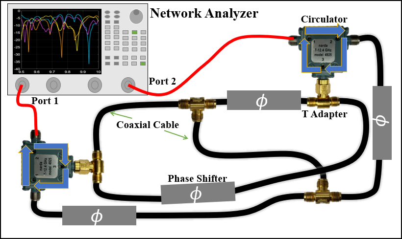
Fig. S1: Schematic of an experimentally realized irregular $M=2$ tetrahedral graph with two channels and non-reciprocal coupling “NRC”. Every node connected to a scattering channel is a circulator, and there are no circulators on internal nodes.

The microwave graphs used in this experiment are constructed with coaxial cables and microwave phase shifters connected to SMA T-type adapters in the topology of a tetrahedron, as shown in Fig 1. This is a standard graph employed in the wave chaos literature [146, 147, 75, 76, 149]. The T-adapters act as the $\nu=4$ nodes of the graph and are the only places where the waves interact. $M$ of the nodes are connected to a Network Analyzer for measurement of the scattering matrix. An ensemble is created through adjusting the setting of four NARDA-Miteq P1507D-SM24 phase shifters, which make up parts of the bonds of the graph, and can be digitally controlled simulatenously through the use of a Trinamic TMCM-6110 PCB. The PCB is connected to the measurement computer that writes the commands, and to a Keithley DC power supply to provide current to the phase shifter stepper motors. Changing the lengths of individual bonds of the graph under the constraints that all six lengths be incommensurate, and that the overall length $L_{e}$ (and hence $\Delta$) remain fixed between realizations, results in a high quality statistical ensemble [139, 143, 144, 145].

The number of scattering channels $M$, the amount of absorption $\eta$, and the presence/absence of reciprocity $\beta$ differentiate the ensembles, which are all made of the same set of $715$ unique phase shifter settings. We also consider a special case of non-reciprocity which we refer to as the “non-reciprocal coupling” (NRC) case, where every port node is a circulator, shown explicitly in Fig. S1. This means waves can only enter and leave the graph through particular paths, and leads to different statistics compared to a graph with circulators only on internal (non-port) nodes of the graph.

S1.2 Higher Dimensional Systems

In addition to the graphs, we also measured the scattering matrix of $\mathcal{D}=2$ a 1/4-bow-tie billiard [126, 153, 154, 131, 158] and $\mathcal{D}=3$ a ray-chaotic cavity (see Fig. S2)[155, 157, 159, 160, 16, 91]. An ensemble is created through adjustment of the voltage applied to varactor diode metasurfaces attached to the walls of the billiard/cavity. The metasurfaces were fabricated by the Johns Hopkins University Applied Physics Laboratory, and vary the reflection phase and amplitude of incident waves, thus altering the boundary conditions [90, 92, 93, 78].

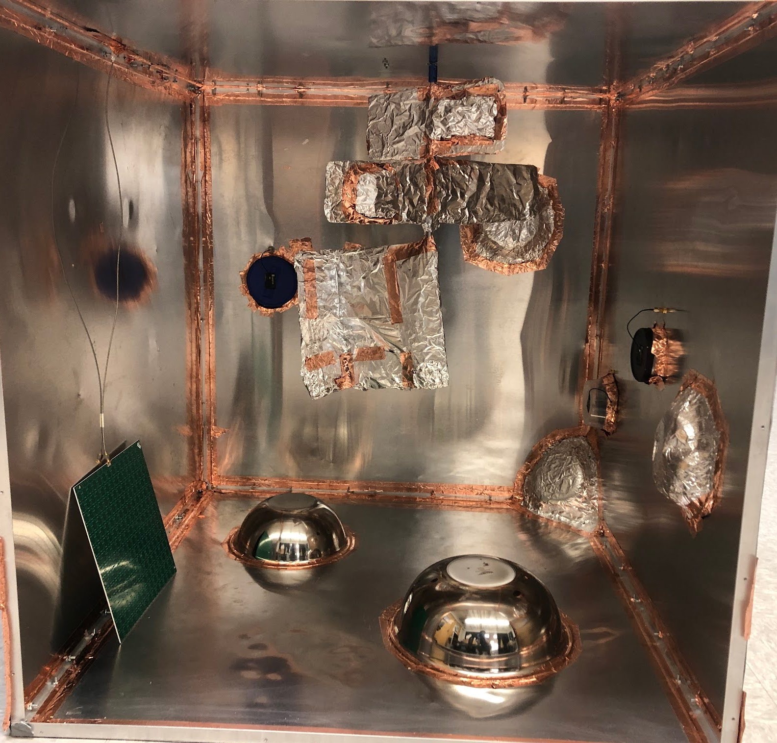
Fig. S2: Photograph of ray-chaotic $\mathcal{D}=3$ dimensional cavity with a tuneable metasurface (green rectangle leaning against the left wall). Line of sight between each port is broken by the use of sheets of Aluminum foil or metal bowls, which also increase the complexity of ray trajectories.

The mean mode spacing $\Delta$ has a more complicated form for higher-dimensional systems, and is no longer frequency independent as in the case of one-dimensional systems. For a two-dimensional billiard, the mean mode spacing can be written as $\Delta=\frac{c}{kA}$ in terms of area $A$ and wavenumber $k$, and for a three-dimensional cavity the mean mode spacing is $\Delta=\frac{\pi c}{2k^{2}V}$, where $V$ is the volume of the scattering system. This complication is off-set by the fact that two and three-dimensional ray-chaotic cavities have statistics that are well described by RMT, unlike graphs.

S1.3 Degree of Absorption

The absorption strength of the systems in this study were in the range of $1.76\leq\eta\leq 49.01$, which extends into what are considered the low- and high-loss regimes. In Fig. 2, it can be seen that the complex $\tau_{WS}$ distributions for systems with larger $\eta$ have the $-3$ power-law tail behavior start at smaller values of $|\text{Re}[\tau_{WS}]|$ and $|\text{Im}[\tau_{WS}]|$. This is similar to a prediction in Ref. [89], that in the ultra-low loss regime ($\eta\ll 1$), an intermediate regime $1\ll M\text{Re}[\tau_{WS}]\ll\frac{1}{\eta}$ exists where the distribution of the real part of the Wigner-Smith time-delay is described by $\mathcal{P}(\text{Re}[\tau_{WS}])\propto\text{Re}[\tau_{WS}]^{-(M\beta)/2-2}$. Notice that this is the exact same form as predicted for the tail of the distribution of the purely real Wigner-Smith time-delay in the Hermitian case.

From this theory, we can see that there should be a transition from Hermitian-like to non-Hermitian behavior for very small $\eta$ values. This may be explained as modes which have small scattering times experience small amounts of attenuation so the system is almost Hermitian. Those that experience large scattering times experience substantial attenuation, even if $\eta$ is small, and therefore we should expect the non-Hermitian $-3$ power-law behavior.

Experimentally, the lowest loss systems were $\mathcal{D}=1$ graphs measured at very low frequencies. The lowest loss ensemble measured has an estimated absorption of $\eta=1.76$ at $2$ GHz, suggesting that we are bounded by the dielectric loss of our coaxial components. Using RMT, the predicted transition is somewhat visible in Fig. S6 when comparing the green curve ($\eta=1.3$) to the blue curve ($\eta=0$) and the dashed red line. The two curves are degenerate for $0.1<\text{Re}[\tau_{WS}]<2$ and are parallel to the dashed red line which characterizes a $-4$ power-law. Note that the finite-loss green curve splits off and becomes parallel to the dashed black line characterizing a $-3$ power-law.

To experimentally observe the predicted transition would likely require a special cryogenic system. That is beyond the scope of this project, and remains an open problem for future research. At the other extreme, we cannot experimentally access the ultra-high loss regime for arbitrarily large $\eta$ values. The tails of the CTD distributions which we are interested in are due to the longest lingering waves. For systems with very large loss, waves that linger for long times are attenuated down into the noise floor of our microwave network analyzer. As a result, we are bounded both above and below on the values of $\eta$ for which we can gather high-quality time-delay statistics.

S1.4 Importance of Frequency Sampling

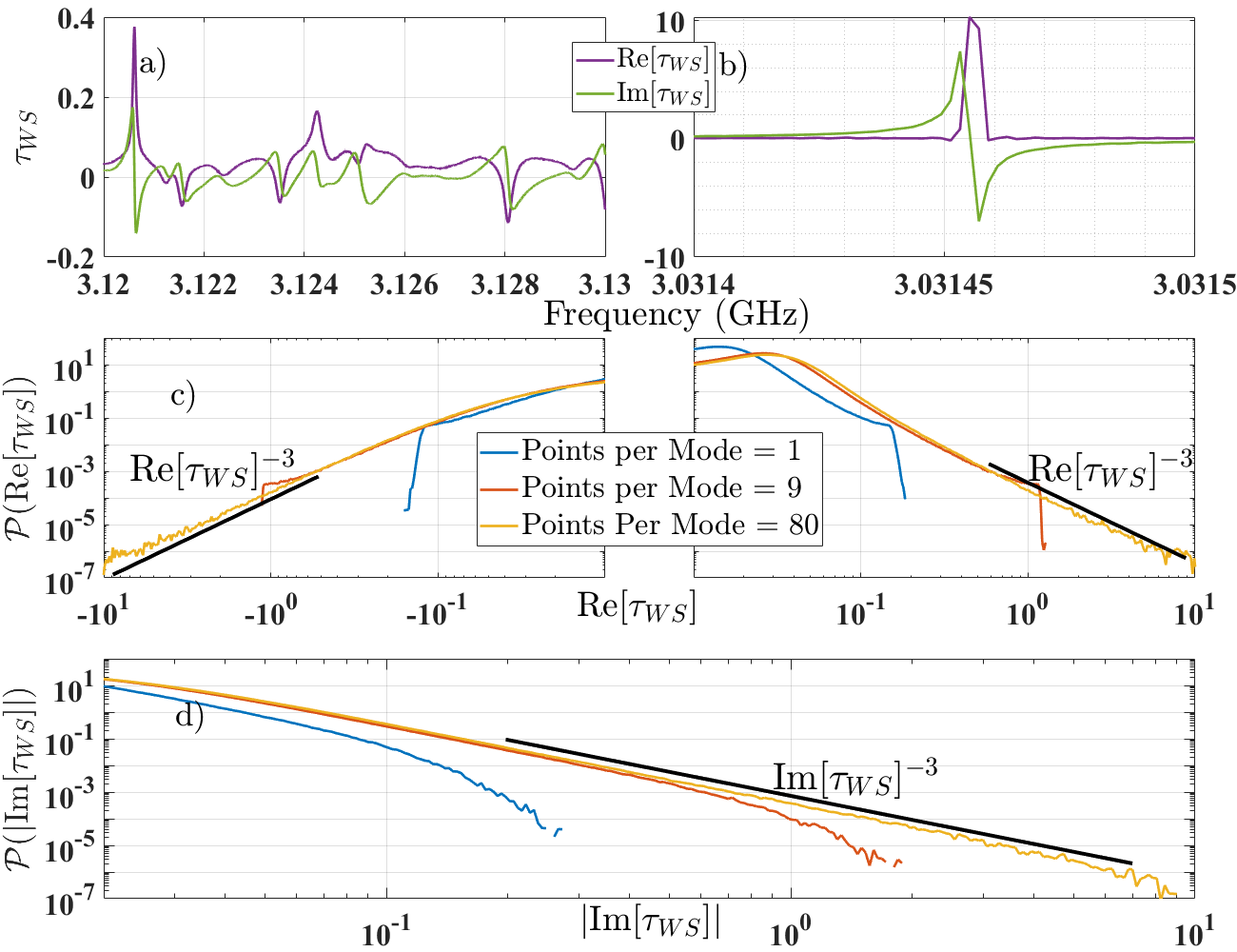
Fig. S3: Complex Wigner-Smith time-delay data from a $\mathcal{D}=3,M=2$ system. (a) $\tau_{WS}$ as a function of frequency. Both real (in purple) and imaginary (in green) components can be positive and negative, with complicated structure as a function of frequency. (b) Zoom in on a mode with large values for the real and imaginary parts of $\tau_{WS}$, showing how the extreme excursions can be very sharp and narrow, requiring high frequency sampling resolution. (c-d) PDFs of Re$[\tau_{WS}]$ and $\lvert$Im$[\tau_{WS}]$$\rvert$ using three different frequency sampling resolutions. The blue and orange curves show that when the sampling in frequency is not fine enough, the extreme time-delays are not represented in the distribution. Black reference line characterizes asymptotic behavior as power-law tail $\tau_{WS}^{-3}$ for the distribution with high sampling resolution.

In Fig. S3(a) we show an example of the complex $\tau_{WS}$ as a function of frequency for one realisation of a three-dimensional microwave cavity. In this frequency range ($3.12-3.13$ GHz), the value of the Wigner-Smith time-delay is small so that the complicated structure of all the modes is visible. The focus of this paper, however, is on the statistics of the tails of the time-delay distributions which correspond to the anomalously long time scattering events. An example of such an event is shown in Fig. S3(b). This extreme event (note the time-delay scale difference between Figs. S3(a) and (b)) takes place over a very small frequency range. Therefore to properly measure these events, it is necessary to measure with high resolution in frequency. This can also be seen from Eqs. 1-3b, which have time-delay as an energy (or equivalently, frequency) derivative of the scattering matrix. Because we are taking a frequency derivative, higher resolution data is needed for time-delay determination, as compared to simply resolving the modes of the system directly from the frequency-dependent $S$-matrix. The curve in Fig. S3(b) is not smooth, showing that this data was undersampled.

In Fig. S3(c-d) we show what the time-delay distributions look like when the frequency resolution is not sufficiently high. The blue curve corresponds to the distribution calculated from data which only has 1 frequency point per mean mode spacing $\Delta$, the orange curve corresponds to 9 points per mode spacing, and the yellow curve corresponds to 80 points per mode spacing. This approximate order of magnitude increase makes clear how important the frequency sampling is to seeing the time-delay distribution tails. It is important to note that $\Delta$ is not the only parameter which determines the density of sampling points. The degree of absorption $\eta$ and the number of scattering channels $M$ both affect how wide the modes are.

S2 Transmission time-delay difference

The transmission time-delay difference is a new quantity introduced for the first time in this paper.

The most basic way to define the transmission difference is with Eq. 3b, which is the difference of the transmission time of one path and its time reversed path. Based on the theory presented in Refs. [25, 27] we can write the complex transmission time-delay difference as a sum over complex transmission zeros $t_{n}$ for each mode of the closed system $n$:

$$\text{Re}[\tau_{\delta T}]=\sum_{n=1}^{N-M}[\frac{\text{Im}[t_{n}]-\eta}{(E-\text{Re}[t_{n}])^{2}+(\text{Im}[t_{n}]-\eta)^{2}}$$ (S1)

$$+\frac{\text{Im}[t_{n}]+\eta}{(E-\text{Re}[t_{n}])^{2}+(\text{Im}[t_{n}]+\eta)^{2}}]$$

$$\text{Im}[\tau_{\delta T}]=-\sum_{n=1}^{N-M}[\frac{E-\text{Re}[t_{n}]}{(E-\text{Re}[t_{n}])^{2}+(\text{Im}[t_{n}]-\eta)^{2}}$$ (S2)

$$-\frac{E-\text{Re}[t_{n}]}{(E-\text{Re}[t_{n}])^{2}+(\text{Im}[t_{n}]+\eta)^{2}}]$$

where $\eta$ is the uniform attenuation, $E$ is the energy, $N$ is the number of modes of the closed system, and $M$ is the number of scattering channels.

One thing that is immediately seen in Fig. 4 is that the peak of $\mathcal{P}(\text{Re}[\tau_{\delta T}])$ is moved away from zero for NRC systems. Whether the peak is moved to a positive or negative values is arbitrary and comes down to which transmission time-delay is subtracted from the other. There is no theory for this qualitatively different behavior, and without more investigation it can’t be said whether or not this is a universal feature; the shifted peak could depend on the structure of the graph, for example.

For a perfectly reciprocal system the PDF of the transmission time-delay difference $\tau_{\delta T}$ is identically a delta function at 0, for both the real and imaginary components. Random Matrix Theory numerics and circuit simulation results show this trivial result, but experimental data does not show this behavior as there are always small differences between measured transmission parameters (i.e. complex $S_{21}\neq S_{12}$ in detail, even for nominally reciprocal systems). Such differences could be caused by imperfect calibration, a bias in the measurement device, small magnetic inclusions in the system, etc and are impossible to fully eliminate. The relative differences between $S_{21}$ and $S_{12}$ are found to be enhanced when the transmission amplitudes are vanishingly small. The transmission zeros cause large spikes in both real and imaginary transmission time-delay difference, which can be seen by inspecting the logarithm in Eq. 3b. If the transmission amplitudes approach zero but one is slightly smaller due to experimental fluctuations, the logarithm can become arbitrarily large, leading to a finite imaginary transmission time-delay difference. The real part of the transmission time-delay difference comes from the phase difference of the transmission parameters, which becomes indeterminate when their magnitudes go to zero. In the case of systems with broken-reciprocity, the transmission time-delay differences are well-defined and non-zero for the vast majority of the data as it is highly unlikely for non-reciprocal transmission amplitudes to both be zero at the same frequency.

S3 Additional Experimental Complex Time-Delay Statistics Results

In this section we provide the distributions of the measured complex reflection and transmission time-delays, all of which also show the same $-3$ power-law tail behavior, independent of $\mathcal{D},M,\beta,\eta$. This is the first experimental demonstration of this superuniversal tail, and we are not aware of any theory which predicts or explains these observations.

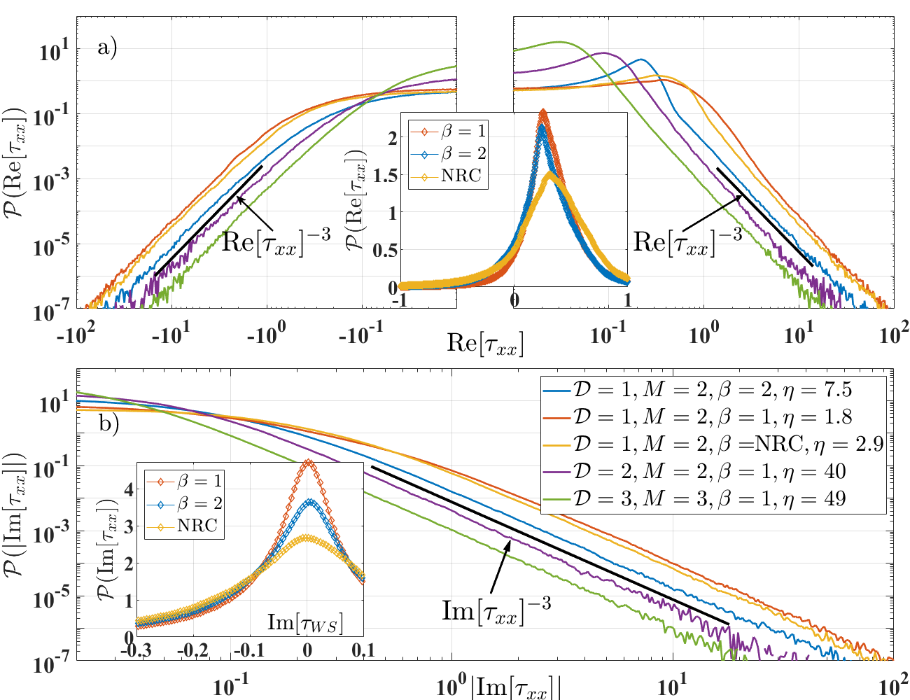
Fig. S4: PDFs of (a) Re$[\tau_{xx}]$ and (b) $\lvert$Im$[\tau_{xx}]$$\rvert$ reflection CTD from select ensembles of chaotic scattering systems with different values for the four parameters $\mathcal{D},M,\beta,\eta$. Insets and reference lines serve the same purpose as in Fig. 2.

Fig. S4 shows the distributions of the complex reflection time-delays $\tau_{xx}$ for five systems with different parameter values, including $M=2$ and $M=3$. As discussed in the main text, the distribution of the tails of the reflection time-delay can be explained by equating it to the Wigner-Smith time-delay of a $M=1$ system, but the distributions of the transmission time-delays $\tau_{xy}$ ($x\neq y$), shown in Fig. S5, require a different analysis to be understood.

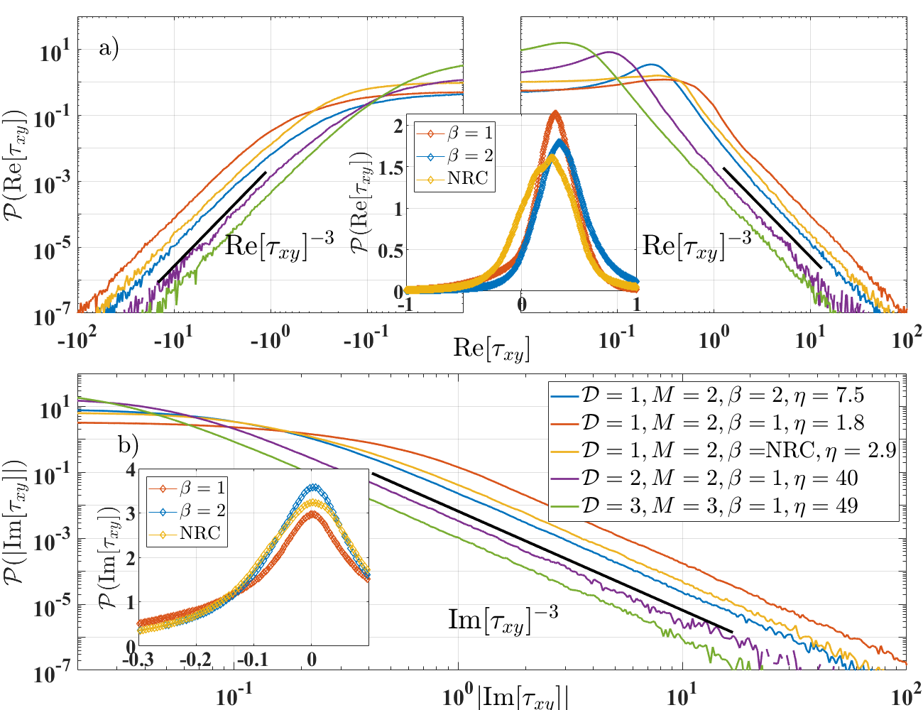
Fig. S5: PDFs of (a) Re$[\tau_{xy}]$ and (b) $\lvert$Im$[\tau_{xy}]$$\rvert$ transmission CTD from select ensembles of chaotic scattering systems with different values for the four parameters $\mathcal{D},M,\beta,\eta$. Insets and reference lines serve the same purpose as in Fig. 2.

S4 Random Matrix Theory Numerics with Loss and Gain

In this section, we demonstrate that numerical data from Random Matrix Theory numerical simulations displays the same superuniversal $-3$ power-law tails for all CTD distributions. The fact that scattering matrices created from random matrix ensembles show the same power-law behavior demonstrates that the power-law tails are generic. We use ensembles of $300$ Gaussian random matrices that are of dimension $10^{5}\crossproduct 10^{5}$. The process of creating the random matrices and using the eigenvalues to generate frequency dependent $S$-matrix data is detailed in Ref. [137], Appendix A of Ref. [136], and Appendix A of Ref. [172]. Accounting for the sampling requirement described in Section S1.4, we calculate the $S$-matrices very finely in the frequency domain, with 336 points per mean mode spacing.

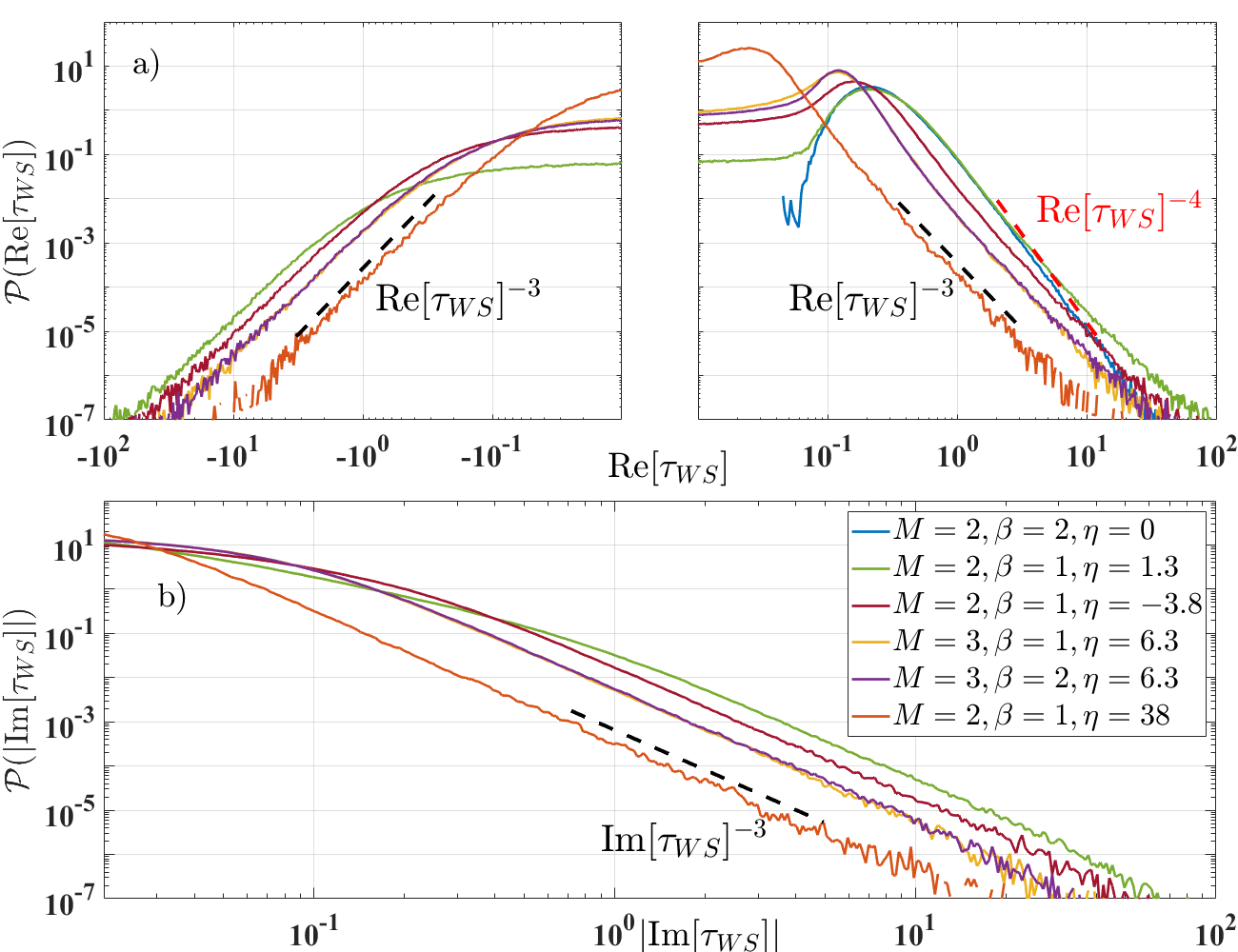
Fig. S6: PDFs of (a) Re$[\tau_{WS}]$ and (b) $\lvert$Im$[\tau_{WS}]$$\rvert$ Wigner-Smith CTD from RMT numerics with different values for $M,\beta,\eta$. Black reference line characterizes asymptotic behavior as power-law tail $\tau_{WS}^{-3}$ for distributions with $\eta>0$. Dashed red line characterizes zero loss asymptotic behavior as $\tau_{WS}^{-\frac{M\beta}{2}-2}$, where $-\frac{M\beta}{2}-2=-4$ for the blue line.

In Fig. S6 we show Wigner-Smith time-delay statistics based on RMT numerics, and the blue curve corresponds to a $M=2,\beta=2,\eta=0$ system, and has a $-4$ power-law tail as predicted for Hermitian scattering systems. The Wigner-Smith time-delay for this system is purely real and positive. The green curve corresponds to a $M=2,\beta=2,\eta=1.3$ system, and is very similar to the lossless case for a range of $\text{Re}[\tau_{WS}]$ before splitting off to have a $-3$ power-law tail. This plot displays the transition region in the distribution discussed in Sec. S1. We also see what was noted in the main text, that the distributions from systems with larger $\eta$ have the power-law tail onset at smaller values of time-delay. The yellow and purple lines both have $M=3,\eta=6.3$, but one corresponds to a reciprocal system and the other does not. The fact that they are essentially on top of each other throughout the entire range plotted shows that $\beta$ has no relevance to the CTD statistics of non-Hermitian systems, whereas it is explicitly dependent on this parameter for Hermitian ones.

With our microwave experiments we are limited to studying only passive lossy systems, but with RMT it is as simple as taking $\eta\rightarrow-\eta$ to simulate a system with gain instead of loss. We show in Supp. Mat. Sec. S4 that at least in the case of RMT numerics the distributions of the CTDs maintain the $-3$ power-law tails even in a system with gain. For the Wigner-Smith time-delay, it is not just the tail that remains the same upon going from loss to gain; in a system with no lumped loss the Wigner-Smith time-delay with uniform absorption $\eta$ is the complex conjugate of the time-delay with gain $-\eta$ ($\tau_{WS,\eta}^{{\dagger}}=\tau_{WS,-\eta}$). This can be seen immediately when writing the Wigner-Smith time-delay in the form of a sum over modes of Lorentzians terms involving the poles and zeros of the $S$-matrix [26]. Because we haven’t done any experimental work on systems with gain, we make no claims on the validity or implications of the distributions with negative $\eta$ values.

Fig. S7: PDFs of (a) Re$[\tau_{xx}]$ and (b) $\lvert$Im$[\tau_{xx}]$$\rvert$ reflection CTD from RMT numerics with different values for $M,\beta,\eta$. Black reference line characterizes asymptotic behavior as power-law tail $\tau_{xx}^{-3}$, common to all distributions.

Fig. S7 shows the complex reflection time-delay distributions calculated through RMT numerics. Even though the blue curve is for a lossless system ($\eta=0$), it still has a $-3$ power-law tail for both its real and imaginary components of $\tau_{xx}$. This follows from the previously stated idea that the reflection time-delay of an $M$ channel system is the same as the Wigner-Smith time-delay of that same system with 1 scattering channel and $M-1$ absorbing channels. Similarly, Fig. S8 shows the distributions for the complex transmission time-delay $\tau_{xy}$ ($x\neq y$), all of which have $-3$ power-law tails. Even for a Hermitian system with a unitary $S$-matrix, the reflection and transmission sub-matrices are generically subunitary and therefore the reflection and transmission time-delays are necessarily complex and display non-Hermitian statistics.

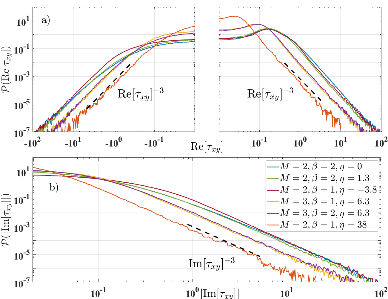
Fig. S8: PDFs of (a) Re$[\tau_{xy}]$ and (b) $\lvert$Im$[\tau_{xy}]$$\rvert$ transmission CTD from RMT numerics with different values for $M,\beta,\eta$. Black reference line characterizes asymptotic behavior as power-law tail $\tau_{xy}^{-3}$, common to all distributions.

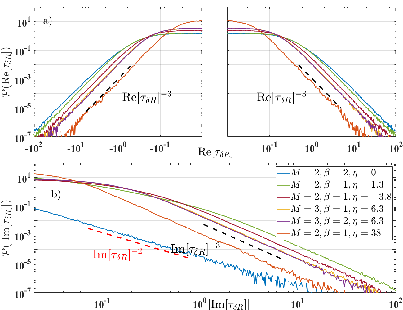
Fig. S9: PDFs of (a) Re$[\tau_{\delta R}]$ and (b) $\lvert$Im$[\tau_{\delta R}]$$\rvert$ reflection time-delay differences from RMT numerics with different values for $M,\beta,\eta$. Black reference line characterizes asymptotic behavior as power-law tail $\tau_{\delta R}^{-3}$, common to all distributions except $\mathcal{P}_{\eta=0}$(Im$[\tau_{\delta R}]$) (lossless case $\eta=0$) which has a $-2$ power-law characterized by the red reference line.

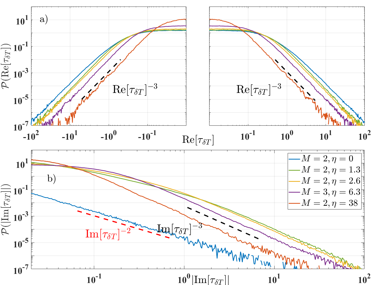
Fig. S10: PDFs of (a) Re$[\tau_{\delta T}]$ and (b) $\lvert$Im$[\tau_{\delta T}]$$\rvert$ transmission time-delay differences from RMT numerics with different values for $M$ and $\eta$. Black reference line characterizes asymptotic behavior as power-law tail $\tau_{\delta R}^{-3}$, common to all distributions except $\mathcal{P}_{\eta=0}($Im$[\tau_{\delta T}]$) (lossless case $\eta=0$) which has a $-2$ power-law characterized by the red reference line.

Figs. S9 and S10 show the distributions of the complex reflection and transmission time-delay differences based on RMT numerics. It is interesting to note the $-2$ power-law for the imaginary component of the reflection and transmission time-delay differences for $\eta=0$ (unitary scattering system) in the broken reciprocity case. For a lossless, and reciprocal $M=2$ system, it is necessary that $S_{11}=S_{22}$ up to a phase, so the reflection time-delay difference is purely real. So in this case we only see an imaginary component of the time-delay differences for $\beta=2$ at zero loss. When the same calculation is done using $M=3$, however, the distributions of the imaginary time differences show $-3$ tails for both $\beta=1$ and $\beta=2$. This is another clear case of how the statistics for a Hermitian system can have strong parameter dependence, but they become simpler in the non-Hermitian case.

S5 Limits of Superuniversal Statistics

In this section, we explore two ways to create deviations from the superuniversal tail behavior that we have discovered. The two effects arise from adding strong lumped loss to the system, and creating very weak coupling between the system and the scattering channels.

S5.1 Lumped Loss and the Disruption of Superuniversal Statistics

A question that might arise is how the CTD statistics are affected by lumped loss as opposed to uniform loss? The answer is rather nuanced, and depends on the relative strength of the two types of absorption. If the lumped attenuation is strong, it can disrupt the expected $-3$ tails for the distributions of the complex time-delays. This is because strong lumped attenuation can effectively deform the cavity and bias the wave propagation. The power-law tails depend on the system being ergodic, which won’t be the case with large lumped attenuation. However, if the system has some uniform attenuation in addition to the lumped loss, then the lumped attenuation won’t be as severe a perturbation, and the statistics reported in this paper can survive.

We attempted to demonstrate this effect experimentally using a graph with an attenuator attached to one internal node. The attenuator is followed by a short circuit, which reflects the wave back through the attenuator and into the graph. A graph with uniform attenuation $\eta=2.7$ thus had a short to ground through either a 4, 8, or 12 dB attenuator attached to one node. In all cases the $-3$ power-law tails survived in all all types of CTD. When the same system was simulated using a circuit model in CST Studio Suite to have uniform attenuation $\eta=0$, the $-3$ power-law tails were not reproduced, even with just a 4 dB load. Simulations with $\eta=2.7$ did produce the $-3$ power-law tails even with an 8 dB lumped attenuator; the threshold of uniform versus lumped attenuation required to maintain the -3 power-law tails is still an open question.

S5.2 Dependence of Statistics on Coupling

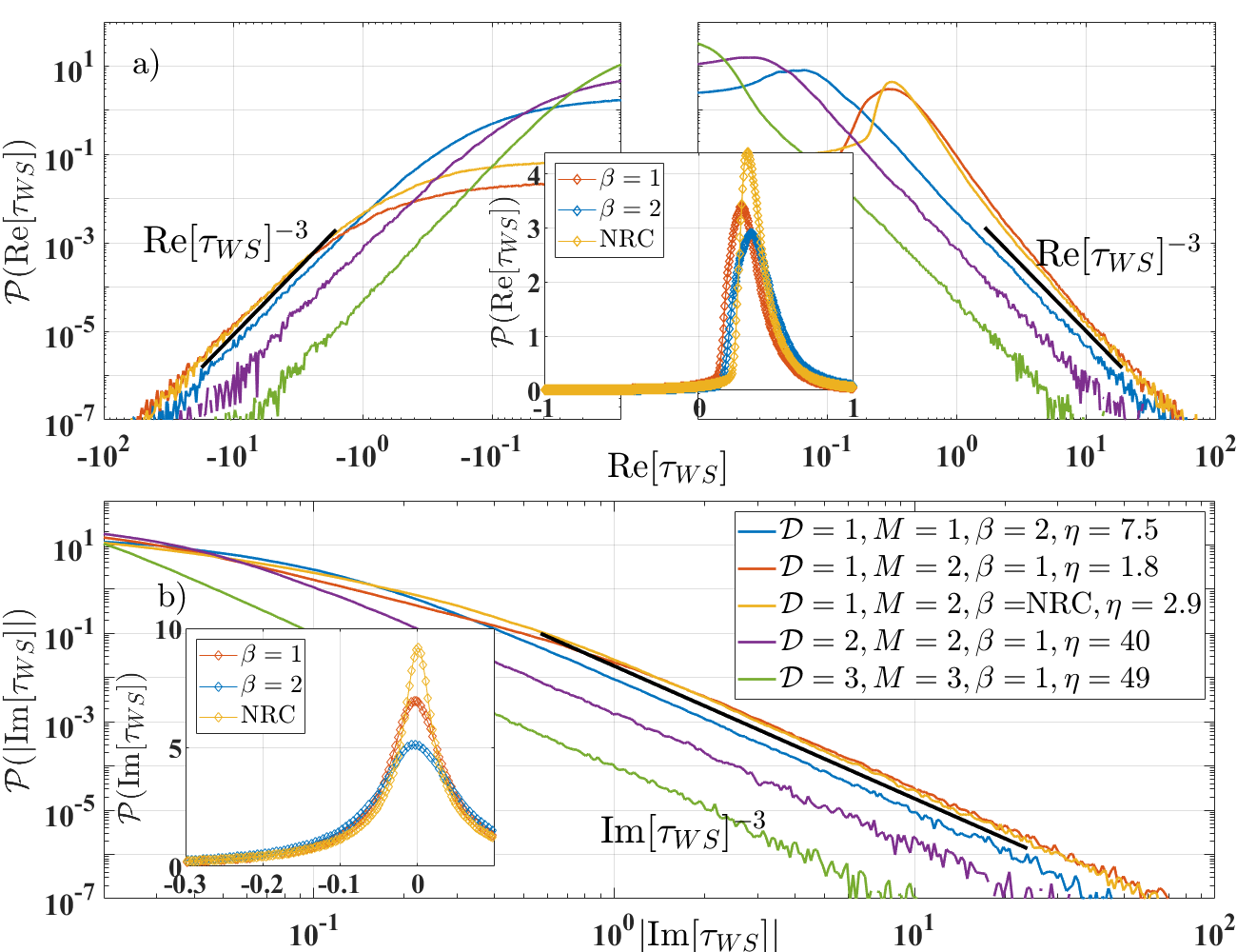
Fig. S11: PDFs of (a) Re$[\tau_{WS}]$ and (b) $\lvert$Im$[\tau_{WS}]$$\rvert$ Wigner-Smith CTD from select measured $S$-matrix ensembles of chaotic scattering systems with different values for the four parameters $\mathcal{D},M,\beta,\eta$, and imperfect coupling. Insets and reference lines serve the same purpose as in Fig. 2.

Here we show the distributions of the CTD calculated from $S$-matrix data with imperfect coupling. This is the same data as shown in the main text and in Sup. Mat. Sec. S3, but the time-delays are calculated using the raw $S$-matrix measured by the network analyzers before RCM-normalization. We find that perfect coupling is not required to observe the superuniversal $-3$ power-law tails, as can be seen in Figs. S11 (Wigner-Smith),  S14 (transmission), and S15 (reflection time-delay difference).

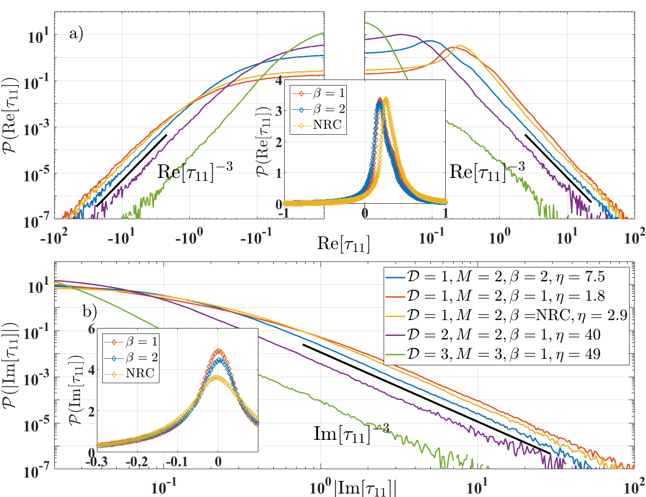
Fig. S12: PDFs of (a) Re$[\tau_{11}]$ and (b) $\lvert$Im$[\tau_{11}]$$\rvert$ port-1 reflection CTD from select ensembles of chaotic scattering systems with different values for the four parameters $\mathcal{D},M,\beta,\eta$, and imperfect coupling. Insets and reference lines serve the same purpose as in Fig. 2.

However, Figs. S12-S13 (reflection time-delays) shows why perfect coupling is important, nonetheless. If the scattering channels are poorly coupled to the cavity, there will be many so called “direct processes,” meaning the waves will immediately be reflected back, and thus not enter the system and suffer a non-zero reflection time-delay. This will cause the reflection time-delay distribution to be very peaked at small time values and not have enough events at large times to show the expected tail behavior. Each channel will have it’s own unique degree of coupling to the system, meaning that the reflection time delay distribution at one port might have the superuniversal $-3$ power-law tail (as seen in Fig. S12) while the distribution from a different channel of the same system might not (as seen in Fig. S12). It is no great surprise that by purposefully making the coupling at certain channels worse than at others, one can comparatively reduce the likelihood of having RSMs at those channels. However, it is still interesting to note that even a system with imperfect coupling may still show the $-3$ power-law tails in some if not all of its reflection time-delay distributions, and seemingly will always have the tail in the other CTD quantities.

We do not yet have a quantifiable measure of exactly how good the coupling must be before the $-3$ power-law tail is able to be seen in the reflection time-delay distribution, and it likely depends on the frequency sampling resolution (See Supp. Mat. Sec. S1.4).

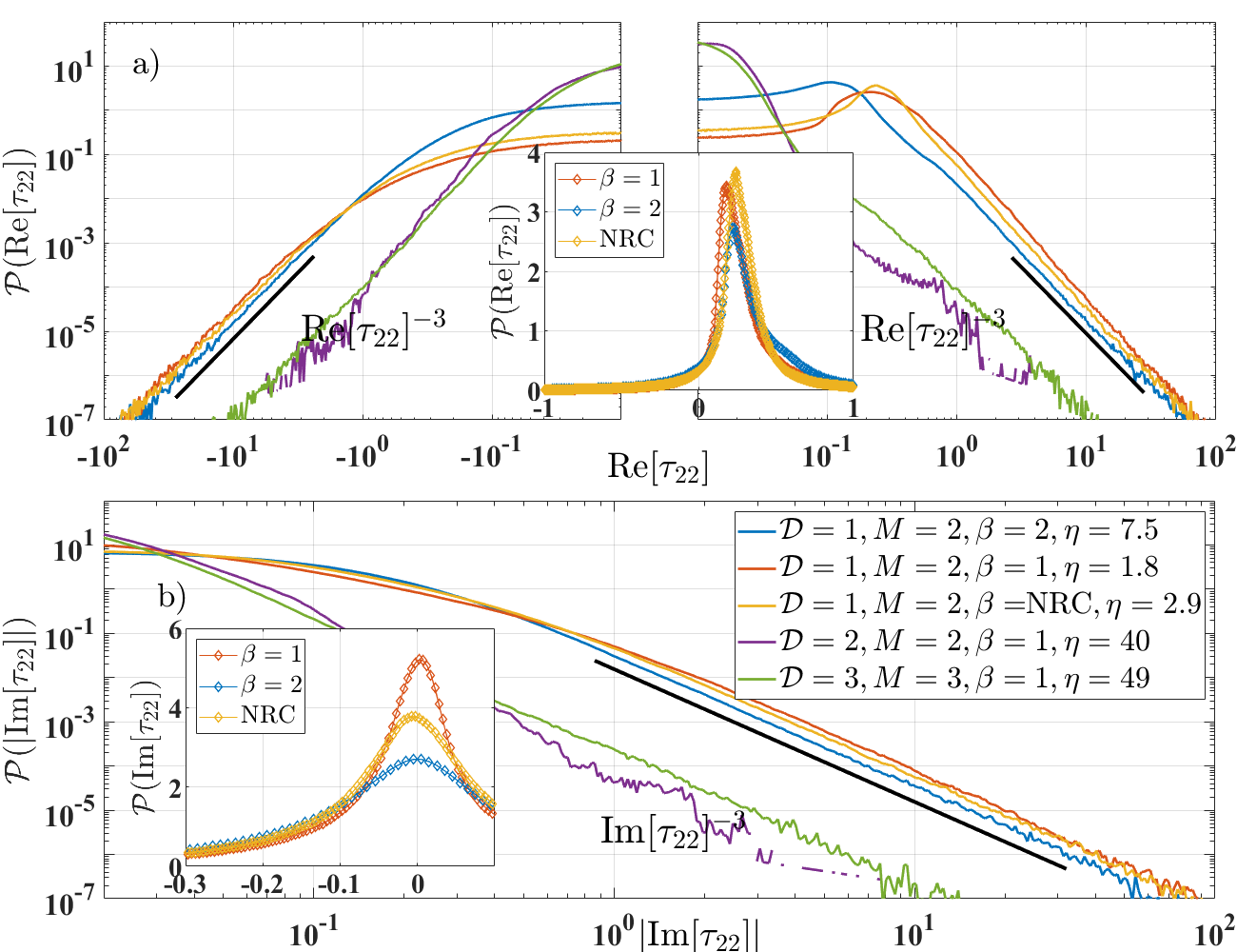
Fig. S13: PDFs of Re$[\tau_{22}]$ and (b) $\lvert$Im$[\tau_{22}]$$\rvert$ port-2 reflection CTD from select ensembles of chaotic scattering systems with different values for the four parameters $\mathcal{D},M,\beta,\eta$, and imperfect coupling. Insets and reference lines serve the same purpose as in Fig. 2.

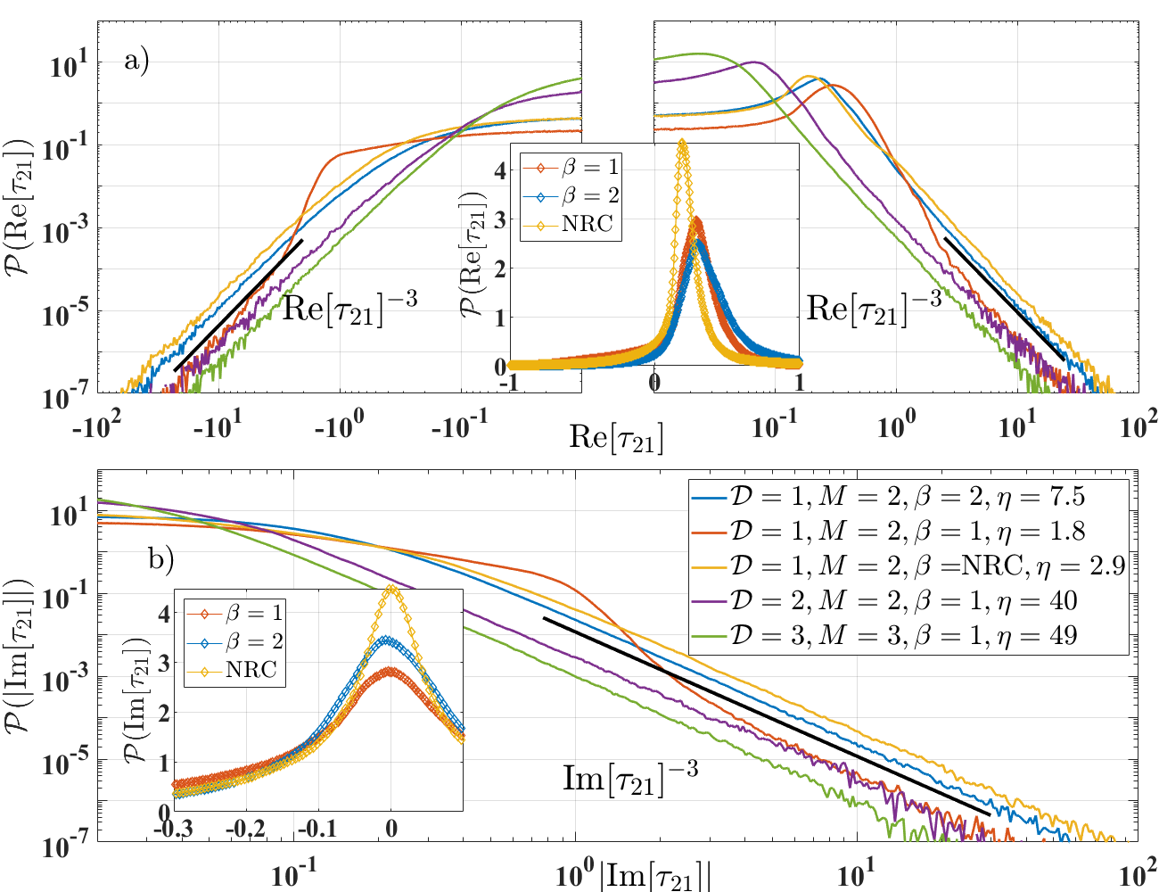
Fig. S14: PDFs of (a) Re$[\tau_{21}]$ and (b) $\lvert$Im$[\tau_{21}]$$\rvert$ transmission CTD from select ensembles of chaotic scattering systems with different values for the four parameters $\mathcal{D},M,\beta,\eta$, and imperfect coupling. Insets and reference lines serve the same purpose as in Fig. 2.

The $\mathcal{D}=1$ graphs have very good coupling even before RCM-normalization because the microwave signals are fed directly into the $M$ nodes using an SMA T-adapter. For the $\mathcal{D}=2$ billiard and $\mathcal{D}=3$ cavity, we have to use antennae which are only well-matched for a small window of the frequency band in which we measure. This is why the green and purple curves are so different from the rest in Figs. S12 and S13. We chose not to show the distributions of the transmission time-delay difference without perfect coupling because all the non-reciprocal systems in this study were graphs, which, as stated before, have very good coupling even before RCM-normalization.

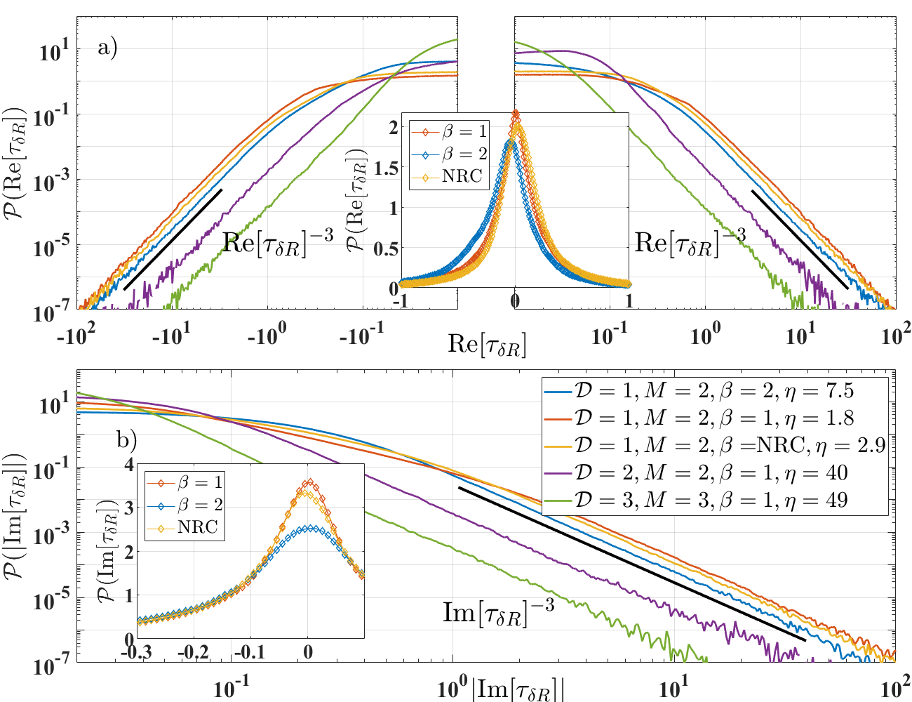
Fig. S15: PDFs of (a) Re$[\tau_{\delta R}]$ and (b) $\lvert$Im$[\tau_{\delta R}]$$\rvert$ reflection time-delay differences from select measured $S$-matrix ensembles of chaotic scattering systems with different values for the four parameters $\mathcal{D},M,\beta,\eta$, and imperfect coupling. Insets and reference lines serve the same purpose as in Fig. 2.

References

- Wigner [1955] E. P. Wigner, Lower limit for the energy derivative of the scattering phase shift, Phys. Rev. 98, 145 (1955).
- Smith [1960] F. T. Smith, Lifetime matrix in collision theory, Phys. Rev. 118, 349 (1960).
- Zhang and Thumm [2011] C.-H. Zhang and U. Thumm, Streaking and wigner time delays in photoemission from atoms and surfaces, Phys. Rev. A 84, 033401 (2011).
- Trabert et al. [2021] D. Trabert, S. Brennecke, K. Fehre, N. Anders, A. Geyer, S. Grundmann, M. S. Schöffler, L. P. H. Schmidt, T. Jahnke, R. Dörner, M. Kunitski, and S. Eckart, Angular dependence of the wigner time delay upon tunnel ionization of h2, Nature Communications 12, 1697 (2021).
- Asano et al. [2016] M. Asano, K. Y. Bliokh, Y. P. Bliokh, A. G. Kofman, R. Ikuta, T. Yamamoto, Y. S. Kivshar, L. Yang, N. Imoto, Ş. K. Özdemir, and F. Nori, Anomalous time delays and quantum weak measurements in optical micro-resonators, Nature Communications 7, 13488 (2016).
- Bourgain et al. [2013] R. Bourgain, J. Pellegrino, S. Jennewein, Y. R. P. Sortais, and A. Browaeys, Direct measurement of the wigner time delay for the scattering of light by a single atom, Opt. Lett. 38, 1963 (2013).
- Deshmukh et al. [2021] P. C. Deshmukh, S. Banerjee, A. Mandal, and S. T. Manson, Eisenbud–wigner–smith time delay in atom–laser interactions, The European Physical Journal Special Topics 230, 4151 (2021).
- Fan and Kahn [2005] S. Fan and J. M. Kahn, Principal modes in multimode waveguides, Opt. Lett. 30, 135 (2005).
- Carpenter et al. [2015] J. Carpenter, B. J. Eggleton, and J. Schröder, Observation of eisenbud–wigner–smith states as principal modes in multimode fibre, Nature Photonics 9, 751 (2015).
- Xiong et al. [2016] W. Xiong, P. Ambichl, Y. Bromberg, B. Redding, S. Rotter, and H. Cao, Spatiotemporal control of light transmission through a multimode fiber with strong mode coupling, Phys. Rev. Lett. 117, 053901 (2016).
- Patel and Michielssen [2021] U. R. Patel and E. Michielssen, Wigner–smith time-delay matrix for electromagnetics: Theory and phenomenology, IEEE Transactions on Antennas and Propagation 69, 902 (2021).
- Mao et al. [2023] Y. Mao, U. R. Patel, and E. Michielssen, Wigner–smith time delay matrix for electromagnetics: Systems with material dispersion and losses, IEEE Transactions on Antennas and Propagation 71, 5266 (2023).
- Rotter et al. [2011] S. Rotter, P. Ambichl, and F. Libisch, Generating particlelike scattering states in wave transport, Phys. Rev. Lett. 106, 120602 (2011).
- Gérardin et al. [2016] B. Gérardin, J. Laurent, P. Ambichl, C. Prada, S. Rotter, and A. Aubry, Particlelike wave packets in complex scattering systems, Phys. Rev. B 94, 014209 (2016).
- Horodynski et al. [2020] M. Horodynski, M. Kühmayer, A. Brandstötter, K. Pichler, Y. V. Fyodorov, U. Kuhl, and S. Rotter, Optimal wave fields for micromanipulation in complex scattering environments, Nature Photonics 14, 149 (2020).
- Frazier et al. [2020] B. W. Frazier, T. M. Antonsen, S. M. Anlage, and E. Ott, Wavefront shaping with a tunable metasurface: Creating cold spots and coherent perfect absorption at arbitrary frequencies, Phys. Rev. Res. 2, 043422 (2020).
- del Hougne et al. [2021a] P. del Hougne, K. B. Yeo, P. Besnier, and M. Davy, On-demand coherent perfect absorption in complex scattering systems: Time delay divergence and enhanced sensitivity to perturbations, Laser & Photonics Reviews 15, 2000471 (2021a).
- Smilansky [2017] U. Smilansky, Delay-time distribution in the scattering of time-narrow wave packets. (i), J. Phys. A: Math. Theor. 50, 215301 (2017).
- Smilansky and Schanze [2018] U. Smilansky and H. Schanze, Delay-time distribution in the scattering of time-narrow wave packets (ii)—quantum graphs, J. Phys. A: Math. Theor. 51, 075302 (2018).
- Brouwer [2003] P. W. Brouwer, Wave function statistics in open chaotic billiards, Phys. Rev. E 68, 046205 (2003).
- Fyodorov and Safonova [2023] Y. V. Fyodorov and E. Safonova, Intensity statistics inside an open wave-chaotic cavity with broken time-reversal invariance, Phys. Rev. E 108, 044206 (2023).
- Fyodorov and Sommers [1997] Y. V. Fyodorov and H.-J. Sommers, Statistics of resonance poles, phase shifts and time delays in quantum chaotic scattering: Random matrix approach for systems with broken time-reversal invariance, Journal of Mathematical Physics 38, 1918 (1997).
- Fyodorov et al. [2017] Y. V. Fyodorov, S. Suwunnarat, and T. Kottos, Distribution of zeros of the s-matrix of chaotic cavities with localized losses and coherent perfect absorption: non-perturbative results, Journal of Physics A: Mathematical and Theoretical 50, 30LT01 (2017).
- Fyodorov [2019] Y. Fyodorov, Reflection time difference as a probe of s-matrix zeroes in chaotic resonance scattering, Acta Physica Polonica A 136, 785 (2019).
- Osman and Fyodorov [2020] M. Osman and Y. V. Fyodorov, Chaotic scattering with localized losses: -matrix zeros and reflection time difference for systems with broken time-reversal invariance, Phys. Rev. E 102, 012202 (2020).
- Chen et al. [2021a] L. Chen, S. M. Anlage, and Y. V. Fyodorov, Generalization of wigner time delay to subunitary scattering systems, Phys. Rev. E 103, L050203 (2021a).
- Chen and Anlage [2022] L. Chen and S. M. Anlage, Use of transmission and reflection complex time delays to reveal scattering matrix poles and zeros: Example of the ring graph, Phys. Rev. E 105, 054210 (2022).
- Genack et al. [1999] A. Z. Genack, P. Sebbah, M. Stoytchev, and B. A. van Tiggelen, Statistics of wave dynamics in random media, Phys. Rev. Lett. 82, 715 (1999).
- Chabanov et al. [2003] A. A. Chabanov, Z. Q. Zhang, and A. Z. Genack, Breakdown of diffusion in dynamics of extended waves in mesoscopic media, Phys. Rev. Lett. 90, 203903 (2003).
- Ambichl et al. [2017] P. Ambichl, A. Brandstötter, J. Böhm, M. Kühmayer, U. Kuhl, and S. Rotter, Focusing inside disordered media with the generalized wigner-smith operator, Phys. Rev. Lett. 119, 033903 (2017).
- Pradhan et al. [2018] P. Pradhan, P. Sahay, and H. M. Almabadi, Derivation of statistics of real delay time from statistics of imaginary delay time using spectroscopic technique in weakly disordered optical media (2018), arXiv:1812.10892 [physics.optics] .
- Huang and Genack [2019] Y. Huang and A. Z. Genack, Delay time inside disordered 1d media, in 2019 Conference on Lasers and Electro-Optics (CLEO) (2019) pp. 1–2.
- del Hougne et al. [2021b] P. del Hougne, K. B. Yeo, P. Besnier, and M. Davy, Coherent wave control in complex media with arbitrary wavefronts, Phys. Rev. Lett. 126, 193903 (2021b).
- Patel et al. [2023] U. R. Patel, Y. Mao, and E. Michielssen, Wigner–Smith time delay matrix for acoustic scattering: Theory and phenomenology, The Journal of the Acoustical Society of America 153, 2769 (2023), https://pubs.aip.org/asa/jasa/article-pdf/153/5/2769/17310479/2769_1_10.0017826.pdf .
- Lehmann et al. [1995] N. Lehmann, D. Savin, V. Sokolov, and H.-J. Sommers, Time delay correlations in chaotic scattering: random matrix approach, Physica D: Nonlinear Phenomena 86, 572 (1995).
- Gopar et al. [1996] V. A. Gopar, P. A. Mello, and M. Büttiker, Mesoscopic capacitors: A statistical analysis, Phys. Rev. Lett. 77, 3005 (1996).
- Misirpashaev et al. [1997] T. S. Misirpashaev, P. W. Brouwer, and C. W. J. Beenakker, Spontaneous emission in chaotic cavities, Phys. Rev. Lett. 79, 1841 (1997).
- Fyodorov et al. [1997] Y. V. Fyodorov, D. V. Savin, and H.-J. Sommers, Parametric correlations of phase shifts and statistics of time delays in quantum chaotic scattering: Crossover between unitary and orthogonal symmetries, Phys. Rev. E 55, R4857 (1997).
- Fyodorov and Alhassid [1998] Y. V. Fyodorov and Y. Alhassid, Photodissociation in quantum chaotic systems: Random-matrix theory of cross-section fluctuations, Phys. Rev. A 58, R3375 (1998).
- van Tiggelen et al. [1999] B. A. van Tiggelen, P. Sebbah, M. Stoytchev, and A. Z. Genack, Delay-time statistics for diffuse waves, Phys. Rev. E 59, 7166 (1999).
- Brouwer et al. [1999] P. W. Brouwer, K. M. Frahm, and C. W. J. Beenakker, Distribution of the quantum mechanical time-delay matrix for a chaotic cavity, Waves in Random Media 9, 91 (1999).
- Savin et al. [2001] D. V. Savin, Y. V. Fyodorov, and H.-J. Sommers, Reducing nonideal to ideal coupling in random matrix description of chaotic scattering: Application to the time-delay problem, Phys. Rev. E 63, 035202 (2001).
- Kottos and Smilansky [2003] T. Kottos and U. Smilansky, Quantum graphs: a simple model for chaotic scattering, Journal of Physics A: Mathematical and General 36, 3501 (2003).
- Mezzadri and Simm [2013] F. Mezzadri and N. J. Simm, Tau-function theory of chaotic quantum transport with = 1, 2, 4, Communications in Mathematical Physics 324, 465 (2013).
- Texier and Majumdar [2013] C. Texier and S. N. Majumdar, Wigner time-delay distribution in chaotic cavities and freezing transition, Phys. Rev. Lett. 110, 250602 (2013).
- Novaes [2015] M. Novaes, Statistics of time delay and scattering correlation functions in chaotic systems. I. Random matrix theory, Journal of Mathematical Physics 56, 062110 (2015).
- Cunden [2015] F. D. Cunden, Statistical distribution of the wigner-smith time-delay matrix moments for chaotic cavities, Phys. Rev. E 91, 060102 (2015).
- Huang et al. [2020] Y. Huang, C. Tian, V. A. Gopar, P. Fang, and A. Z. Genack, Invariance principle for wave propagation inside inhomogeneously disordered materials, Phys. Rev. Lett. 124, 057401 (2020).
- Šeba et al. [1996] P. Šeba, K. Życzkowski, and J. Zakrzewski, Statistical properties of random scattering matrices, Physical Review E 54, 2438 (1996).
- Fyodorov and Sommers [1996] Y. V. Fyodorov and H.-J. Sommers, Parametric correlations of scattering phase shifts and fluctuations of delay times in few-channel chaotic scattering, Phys. Rev. Lett. 76, 4709 (1996).
- Brouwer et al. [1997] P. W. Brouwer, K. M. Frahm, and C. W. J. Beenakker, Quantum mechanical time-delay matrix in chaotic scattering, Phys. Rev. Lett. 78, 4737 (1997).
- Savin and Sommers [2003] D. V. Savin and H.-J. Sommers, Delay times and reflection in chaotic cavities with absorption, Phys. Rev. E 68, 036211 (2003).
- Ossipov and Fyodorov [2005] A. Ossipov and Y. V. Fyodorov, Statistics of delay times in mesoscopic systems as a manifestation of eigenfunction fluctuations, Phys. Rev. B 71, 125133 (2005).
- Kottos [2005] T. Kottos, Statistics of resonances and delay times in random media: beyond random matrix theory, Journal of Physics A: Mathematical and General 38, 10761 (2005).
- Grabsch et al. [2018] A. Grabsch, D. V. Savin, and C. Texier, Wigner–smith time-delay matrix in chaotic cavities with non-ideal contacts, Journal of Physics A: Mathematical and Theoretical 51, 404001 (2018).
- Grabsch [2019] A. Grabsch, Distribution of the wigner–smith time-delay matrix for chaotic cavities with absorption and coupled coulomb gases, Journal of Physics A: Mathematical and Theoretical 53, 025202 (2019).
- Dyson [1962] F. J. Dyson, The Threefold Way. Algebraic Structure of Symmetry Groups and Ensembles in Quantum Mechanics, Journal of Mathematical Physics 3, 1199 (1962).
- Texier [2016] C. Texier, Wigner time delay and related concepts: Application to transport in coherent conductors, Physica E: Low-dimensional Systems and Nanostructures 82, 16 (2016), frontiers in quantum electronic transport - In memory of Markus Büttiker.
- Fyodorov and Savin [2004] Y. V. Fyodorov and D. V. Savin, Statistics of impedance, local density of states, and reflection in quantum chaotic systems with absorption, Journal of Experimental and Theoretical Physics Letters 80, 725 (2004).
- Savin et al. [2005] D. V. Savin, H.-J. Sommers, and Y. V. Fyodorov, Universal statistics of the local green’s function in wave chaotic systems with absorption, Journal of Experimental and Theoretical Physics Letters 82, 544 (2005).
- Fyodorov et al. [2005] Y. V. Fyodorov, D. V. Savin, and H.-J. Sommers, Scattering, reflection and impedance of waves in chaotic and disordered systems with absorption, Journal of Physics A: Mathematical and General 38, 10731 (2005).
- Xing Zheng and Ott [2006a] T. M. A. Xing Zheng and E. Ott, Statistics of impedance and scattering matrices of chaotic microwave cavities with multiple ports, Electromagnetics 26, 37 (2006a).
- Xing Zheng and Ott [2006b] T. M. A. Xing Zheng and E. Ott, Statistics of impedance and scattering matrices in chaotic microwave cavities: Single channel case, Electromagnetics 26, 3 (2006b).
- Zheng et al. [2006] X. Zheng, S. Hemmady, T. M. Antonsen, S. M. Anlage, and E. Ott, Characterization of fluctuations of impedance and scattering matrices in wave chaotic scattering, Phys. Rev. E 73, 046208 (2006).
- Hemmady et al. [2006a] S. Hemmady, J. Hart, X. Zheng, T. M. Antonsen, E. Ott, and S. M. Anlage, Experimental test of universal conductance fluctuations by means of wave-chaotic microwave cavities, Phys. Rev. B 74, 195326 (2006a).
- Hemmady et al. [2006b] S. Hemmady, X. Zheng, T. M. Antonsen, E. Ott, and S. M. Anlage, Aspects of the scattering and impedance properties of chaotic microwave cavities, Acta Physica Polonica A 109, 65 (2006b).
- Hemmady et al. [2006c] S. Hemmady, X. Zheng, J. Hart, T. M. Antonsen, E. Ott, and S. M. Anlage, Universal properties of two-port scattering, impedance, and admittance matrices of wave-chaotic systems, Phys. Rev. E 74, 036213 (2006c).
- Yeh et al. [2013] J.-H. Yeh, Z. Drikas, J. G. Gil, S. Hong, B. Taddese, E. Ott, T. Antonsen, T. Andreadis, and S. Anlage, Impedance and scattering variance ratios of complicated wave scattering systems in the low loss regime, Acta Physica Polonica A 124, 1045 (2013).
- Beenakker and Brouwer [2001] C. Beenakker and P. Brouwer, Distribution of the reflection eigenvalues of a weakly absorbing chaotic cavity, Physica E: Low-dimensional Systems and Nanostructures 9, 463 (2001), proceedings of an International Workshop and Seminar on the Dynamics of Complex Systems.
- Fyodorov [2003] Y. V. Fyodorov, Induced vs. spontaneous breakdown of s-matrix unitarity: Probability of no return in quantum chaotic and disordered systems, Journal of Experimental and Theoretical Physics Letters 78, 250 (2003).
- Novaes and Kuipers [2023] M. Novaes and J. Kuipers, Effect of a tunnel barrier on time delay statistics, Phys. Rev. E 108, 034201 (2023).
- Novaes [2023] M. Novaes, Time delay statistics for chaotic cavities with absorption, Journal of Statistical Physics 190, 182 (2023).
- Böhm et al. [2018] J. Böhm, A. Brandstötter, P. Ambichl, S. Rotter, and U. Kuhl, In situ realization of particlelike scattering states in a microwave cavity, Phys. Rev. A 97, 021801 (2018).
- Bredol [2021] P. Bredol, Nonreciprocity of the wave-packet scattering delay in ballistic two-terminal devices, Phys. Rev. B 103, 035404 (2021).
- Li et al. [2017] H. Li, S. Suwunnarat, R. Fleischmann, H. Schanz, and T. Kottos, Random matrix theory approach to chaotic coherent perfect absorbers, Phys. Rev. Lett. 118, 044101 (2017).
- Chen et al. [2020] L. Chen, T. Kottos, and S. M. Anlage, Perfect absorption in complex scattering systems with or without hidden symmetries, Nature Communications 11, 5826 (2020).
- F. Imani et al. [2020] M. F. Imani, D. R. Smith, and P. del Hougne, Perfect absorption in a disordered medium with programmable meta-atom inclusions, Advanced Functional Materials 30, 2005310 (2020).
- Erb et al. [2024] J. Erb, D. Shrekenhamer, T. Sleasman, T. Antonsen, and S. Anlage, Control of the scattering properties of complex systems by means of tunable metasurfaces, Acta Physica Polonica A ISSN 1898-794X 144, 421 (2024).
- Faul et al. [2024] F. T. Faul, L. Cronier, A. Alhulaymi, A. D. Stone, and P. del Hougne, Agile free-form signal filtering with a chaotic-cavity-backed non-local programmable metasurface (2024), arXiv:2407.00054 [physics.app-ph] .
- Huang et al. [2022] Y. Huang, Y. Kang, and A. Z. Genack, Wave excitation and dynamics in non-hermitian disordered systems, Phys. Rev. Res. 4, 013102 (2022).
- Sol et al. [2023] J. Sol, A. Alhulaymi, A. D. Stone, and P. del Hougne, Reflectionless programmable signal routers, Science Advances 9, eadf0323 (2023), https://www.science.org/doi/pdf/10.1126/sciadv.adf0323 .
- Jiang et al. [2024] X. Jiang, S. Yin, H. Li, J. Quan, H. Goh, M. Cotrufo, J. Kullig, J. Wiersig, and A. Alù, Coherent control of chaotic optical microcavity with reflectionless scattering modes, Nature Physics 20, 109 (2024).
- Boyd and Gauthier [2002] R. Boyd and D. Gauthier, ”slow” and ”fast” light, Progress in Optics 43 (2002).
- Shi et al. [2007] Z. Shi, R. W. Boyd, D. J. Gauthier, and C. C. Dudley, Enhancing the spectral sensitivity of interferometers using slow-light media, Opt. Lett. 32, 915 (2007).
- Bhagat and Gaikwad [2021] D. Bhagat and M. Gaikwad, A review on production of slow light with material characterization, Materials Today: Proceedings 43, 1780 (2021), international Conference on Advanced Materials Behavior and Characterization (ICAMBC 2020).
- Lin et al. [2011] Z. Lin, H. Ramezani, T. Eichelkraut, T. Kottos, H. Cao, and D. N. Christodoulides, Unidirectional invisibility induced by -symmetric periodic structures, Phys. Rev. Lett. 106, 213901 (2011).
- Kurter et al. [2011] C. Kurter, P. Tassin, L. Zhang, T. Koschny, A. P. Zhuravel, A. V. Ustinov, S. M. Anlage, and C. M. Soukoulis, Classical analogue of electromagnetically induced transparency with a metal-superconductor hybrid metamaterial, Phys. Rev. Lett. 107, 043901 (2011).
- Peng et al. [2014] B. Peng, Ş. K. Özdemir, F. Lei, F. Monifi, M. Gianfreda, G. L. Long, S. Fan, F. Nori, C. M. Bender, and L. Yang, Parity–time-symmetric whispering-gallery microcavities, Nature Physics 10, 394 (2014).
- Chen et al. [2021b] L. Chen, S. M. Anlage, and Y. V. Fyodorov, Statistics of complex wigner time delays as a counter of -matrix poles: Theory and experiment, Phys. Rev. Lett. 127, 204101 (2021b).
- Chen et al. [2016] H.-T. Chen, A. J. Taylor, and N. Yu, A review of metasurfaces: physics and applications, Reports on Progress in Physics 79, 076401 (2016).
- Frazier et al. [2022] B. W. Frazier, T. M. Antonsen, S. M. Anlage, and E. Ott, Deep-learning estimation of complex reverberant wave fields with a programmable metasurface, Physical Review Applied 17, 024027 (2022).
- Elsawy et al. [2023] M. Elsawy, C. Kyrou, E. Mikheeva, R. Colom, J.-Y. Duboz, K. Z. Kamali, S. Lanteri, D. Neshev, and P. Genevet, Universal active metasurfaces for ultimate wavefront molding by manipulating the reflection singularities, Laser & Photonics Reviews 17, 2200880 (2023).
- Sleasman et al. [2023] T. Sleasman, R. Duggan, R. S. Awadallah, and D. Shrekenhamer, Dual-resonance dynamic metasurface for independent magnitude and phase modulation, Phys. Rev. Appl. 20, 014004 (2023).
- Stein et al. [2022] M. Stein, S. Keller, Y. Luo, and O. Ilic, Shaping contactless radiation forces through anomalous acoustic scattering, Nature Communications 13, 6533 (2022).
- Huang et al. [2024] L. Huang, S. Huang, C. Shen, S. Yves, A. S. Pilipchuk, X. Ni, S. Kim, Y. K. Chiang, D. A. Powell, J. Zhu, Y. Cheng, Y. Li, A. F. Sadreev, A. Alù, and A. E. Miroshnichenko, Acoustic resonances in non-hermitian open systems, Nature Reviews Physics 6, 11 (2024).
- Cummer et al. [2016] S. A. Cummer, J. Christensen, and A. Alù, Controlling sound with acoustic metamaterials, Nature Reviews Materials 1, 16001 (2016).
- Chong et al. [2010] Y. D. Chong, L. Ge, H. Cao, and A. D. Stone, Coherent perfect absorbers: Time-reversed lasers, Phys. Rev. Lett. 105, 053901 (2010).
- Wan et al. [2011] W. Wan, Y. Chong, L. Ge, H. Noh, A. D. Stone, and H. Cao, Time-reversed lasing and interferometric control of absorption, Science 331, 889 (2011), https://www.science.org/doi/pdf/10.1126/science.1200735 .
- Pichler et al. [2019] K. Pichler, M. Kühmayer, J. Böhm, A. Brandstötter, P. Ambichl, U. Kuhl, and S. Rotter, Random anti-lasing through coherent perfect absorption in a disordered medium, Nature 567, 351 (2019).
- Verbaarschot et al. [1985] J. Verbaarschot, H. Weidenmüller, and M. Zirnbauer, Grassmann integration in stochastic quantum physics: The case of compound-nucleus scattering, Physics Reports 129, 367 (1985).
- Sokolov and Zelevinsky [1989] V. Sokolov and V. Zelevinsky, Dynamics and statistics of unstable quantum states, Nuclear Physics A 504, 562 (1989).
- Fyodorov and Savin [2011] Y. V. Fyodorov and D. V. Savin, Resonance scattering of waves in chaotic systems, in The Oxford Handbook of Random Matrix Theory, edited by G. Akemann, J. Baik, and P. D. Francesco (Oxford University Press, 2011) pp. 703–722.
- Kuhl et al. [2013] U. Kuhl, O. Legrand, and F. Mortessagne, Microwave experiments using open chaotic cavities in the realm of the effective hamiltonian formalism, Fortschritte der Physik 61, 404 (2013).
- Schomerus [2017] H. Schomerus, Random matrix approaches to open quantum systems, in Stochastic Processes and Random Matrices: Lecture Notes of the Les Houches Summer School 2015, edited by G. Schehr, A. Altland, Y. V. Fyodorov, N. O’Connell, and L. F. Cugliandolo (Oxford University Press, 2017) pp. 409–473.
- Kang and Genack [2021a] Y. Kang and A. Z. Genack, Transmission zeros with topological symmetry in complex systems, Phys. Rev. B 103, L100201 (2021a).
- Fisher and Lee [1981] D. S. Fisher and P. A. Lee, Relation between conductivity and transmission matrix, Phys. Rev. B 23, 6851 (1981).
- Rotter and Gigan [2017] S. Rotter and S. Gigan, Light fields in complex media: Mesoscopic scattering meets wave control, Rev. Mod. Phys. 89, 015005 (2017).
- Ma and Anlage [2023] S. Ma and S. M. Anlage, Experimental realization of anti-unitary wave-chaotic photonic topological insulator graphs showing kramers degeneracy and symplectic ensemble statistics, Advanced Optical Materials n/a, 2301852 (2023).
- Sebbah et al. [1999] P. Sebbah, O. Legrand, and A. Z. Genack, Fluctuations in photon local delay time and their relation to phase spectra in random media, Phys. Rev. E 59, 2406 (1999).
- van Bemmel et al. [2001] K. J. H. van Bemmel, H. Schomerus, and C. W. J. Beenakker, Single-mode delay time statistics for scattering by a chaotic cavity, Physica Scripta 2001, 278 (2001).
- Białous et al. [2021] M. Białous, P. Dulian, A. Sawicki, and L. Sirko, Delay-time distribution in the scattering of short gaussian pulses in microwave networks, Phys. Rev. E 104, 024223 (2021).
- Genack et al. [2024] A. Z. Genack, Y. Huang, A. Maor, and Z. Shi, Velocities of transmission eigenchannels and diffusion, Nature Communications 15, 2606 (2024).
- Chen et al. [2024] L. Chen, I. L. Giovannelli, N. Shaibe, and S. M. Anlage, Asymmetric transmission through a classical analogue of the aharonov-bohm ring, Phys. Rev. B 110, 045103 (2024).
- Kang and Genack [2021b] Y. Kang and A. Z. Genack, Transmission zeros with topological symmetry in complex systems, Phys. Rev. B 103, L100201 (2021b).
- So et al. [1995] P. So, S. M. Anlage, E. Ott, and R. N. Oerter, Wave chaos experiments with and without time reversal symmetry: Gue and goe statistics, Phys. Rev. Lett. 74, 2662 (1995).
- Stoffregen et al. [1995] U. Stoffregen, J. Stein, H.-J. Stöckmann, M. Kuś, and F. Haake, Microwave billiards with broken time reversal symmetry, Phys. Rev. Lett. 74, 2666 (1995).
- Wu et al. [1998] D. H. Wu, J. S. A. Bridgewater, A. Gokirmak, and S. M. Anlage, Probability amplitude fluctuations in experimental wave chaotic eigenmodes with and without time-reversal symmetry, Physical Review Letters 81, 2890 (1998).
- Chung et al. [2000] S. H. Chung, A. Gokirmak, D. H. Wu, J. S. A. Bridgewater, E. Ott, T. M. Antonsen, and S. M. Anlage, Measurement of wave chaotic eigenfunctions in the time-reversal symmetry-breaking crossover regime, Physical Review Letters 85, 2482 (2000).
- Schanze et al. [2005] H. Schanze, H.-J. Stöckmann, M. Martínez-Mares, and C. H. Lewenkopf, Universal transport properties of open microwave cavities with and without time-reversal symmetry, Phys. Rev. E 71, 016223 (2005).
- Ławniczak et al. [2009] M. Ławniczak, S. Bauch, O. Hul, and L. Sirko, Experimental investigation of properties of hexagon networks with and without time reversal symmetry, Physica Scripta 2009, 014050 (2009).
- Ławniczak et al. [2010] M. Ławniczak, S. Bauch, O. Hul, and L. Sirko, Experimental investigation of the enhancement factor for microwave irregular networks with preserved and broken time reversal symmetry in the presence of absorption, Phys. Rev. E 81, 046204 (2010).
- Ławniczak et al. [2011] M. Ławniczak, S. Bauch, O. Hul, and L. Sirko, Experimental investigation of the enhancement factor and the cross-correlation function for graphs with and without time-reversal symmetry: the open system case, Physica Scripta 2011, 014014 (2011).
- Ławniczak and Sirko [2019] M. Ławniczak and L. Sirko, Investigation of the diagonal elements of the wigner’s reaction matrix for networks with violated time reversal invariance, Scientific Reports 9, 5630 (2019).
- Zhang et al. [2023] X. Zhang, W. Zhang, J. Che, and B. Dietz, Experimental test of the rosenzweig-porter model for the transition from poisson to gaussian unitary ensemble statistics, Phys. Rev. E 108, 044211 (2023).
- Doron et al. [1990] E. Doron, U. Smilansky, and A. Frenkel, Experimental demonstration of chaotic scattering of microwaves, Phys. Rev. Lett. 65, 3072 (1990).
- Stöckmann and Stein [1990] H.-J. Stöckmann and J. Stein, “quantum” chaos in billiards studied by microwave absorption, Phys. Rev. Lett. 64, 2215 (1990).
- Stöckmann [1999] H.-J. Stöckmann, Quantum Chaos An Introduction (Cambridge University Press, 1999).
- Richter [2001] A. Richter, Wave dynamical chaos: an experimental approach in billiards, Physica Scripta 2001, 212 (2001).
- Hul et al. [2012] O. Hul, M. Ławniczak, S. Bauch, A. Sawicki, M. Kuś, and L. Sirko, Are scattering properties of graphs uniquely connected to their shapes?, Phys. Rev. Lett. 109, 040402 (2012).
- Gradoni et al. [2014] G. Gradoni, J.-H. Yeh, B. Xiao, T. M. Antonsen, S. M. Anlage, and E. Ott, Predicting the statistics of wave transport through chaotic cavities by the random coupling model: A review and recent progress, Wave Motion 51, 606 (2014).
- Dietz and Richter [2015] B. Dietz and A. Richter, Quantum and wave dynamical chaos in superconducting microwave billiards, Chaos: An Interdisciplinary Journal of Nonlinear Science 25, 097601 (2015).
- Hemmady et al. [2005a] S. Hemmady, X. Zheng, E. Ott, T. M. Antonsen, and S. M. Anlage, Universal impedance fluctuations in wave chaotic systems, Phys. Rev. Lett. 94, 014102 (2005a).
- Hart et al. [2009] J. A. Hart, T. M. Antonsen, and E. Ott, Effect of short ray trajectories on the scattering statistics of wave chaotic systems, Phys. Rev. E 80, 041109 (2009).
- Yeh et al. [2010] J.-H. Yeh, J. A. Hart, E. Bradshaw, T. M. Antonsen, E. Ott, and S. M. Anlage, Experimental examination of the effect of short ray trajectories in two-port wave-chaotic scattering systems, Phys. Rev. E 82, 041114 (2010).
- Ławniczak et al. [2012] M. Ławniczak, S. Bauch, O. Hul, and L. Sirko, Experimental investigation of microwave networks simulating quantum chaotic systems: the role of direct processes, Physica Scripta 2012, 014018 (2012).
- Hemmady et al. [2012] S. Hemmady, T. M. Antonsen, E. Ott, and S. M. Anlage, Statistical prediction and measurement of induced voltages on components within complicated enclosures: A wave-chaotic approach, IEEE Transactions on Electromagnetic Compatibility 54, 758 (2012).
- Lee et al. [2013] M.-J. Lee, T. M. Antonsen, and E. Ott, Statistical model of short wavelength transport through cavities with coexisting chaotic and regular ray trajectories, Phys. Rev. E 87, 062906 (2013).
- Aurégan and Pagneux [2016] Y. Aurégan and V. Pagneux, Acoustic scattering in duct with a chaotic cavity, Acta Acustica united with Acustica 102, 869 (2016).
- Dietz et al. [2017] B. Dietz, V. Yunko, M. Białous, S. Bauch, M. Ławniczak, and L. Sirko, Nonuniversality in the spectral properties of time-reversal-invariant microwave networks and quantum graphs, Phys. Rev. E 95, 052202 (2017).
- Lyuboshitz [1977] V. L. Lyuboshitz, On collision duration in the presence of strong overlapping resonance levels, Phys. Lett. B 72, 41 (1977).
- Pierrat et al. [2014] R. Pierrat, P. Ambichl, S. Gigan, A. Haber, R. Carminati, and S. Rotter, Invariance property of wave scattering through disordered media, Proceedings of the National Academy of Sciences 111, 17765 (2014).
- Rehemanjiang et al. [2018] A. Rehemanjiang, M. Richter, U. Kuhl, and H.-J. Stöckmann, Spectra and spectral correlations of microwave graphs with symplectic symmetry, Phys. Rev. E 97, 022204 (2018).
- Che et al. [2021] J. Che, J. Lu, X. Zhang, B. Dietz, and G. Chai, Missing-level statistics in classically chaotic quantum systems with symplectic symmetry, Phys. Rev. E 103, 042212 (2021).
- Che et al. [2022] J. Che, X. Zhang, W. Zhang, B. Dietz, and G. Chai, Fluctuation properties of the eigenfrequencies and scattering matrix of closed and open unidirectional graphs with chaotic wave dynamics, Phys. Rev. E 106, 014211 (2022).
- Ławniczak et al. [2023] M. Ławniczak, A. Akhshani, O. Farooq, M. Białous, S. Bauch, B. Dietz, and L. Sirko, Distributions of the wigner reaction matrix for microwave networks with symplectic symmetry in the presence of absorption, Phys. Rev. E 107, 024203 (2023).
- Kottos and Smilansky [1997] T. Kottos and U. Smilansky, Quantum chaos on graphs, Phys. Rev. Lett. 79, 4794 (1997).
- Hul et al. [2004] O. Hul, S. Bauch, P. Pakoński, N. Savytskyy, K. Życzkowski, and L. Sirko, Experimental simulation of quantum graphs by microwave networks, Phys. Rev. E 69, 056205 (2004).
- Fu et al. [2017] Z. Fu, T. Koch, T. Antonsen, and S. Anlage, Experimental study of quantum graphs with simple microwave networks: Non-universal features, Acta Phys. Pol. A 132, 1655 (2017).
- Hofmann et al. [2021] T. Hofmann, J. Lu, U. Kuhl, and H.-J. Stöckmann, Spectral duality in graphs and microwave networks, Phys. Rev. E 104, 045211 (2021).
- Lu et al. [2023] J. Lu, T. Hofmann, U. Kuhl, and H.-J. Stöckmann, Implications of spectral interlacing for quantum graphs, Entropy 25, 109 (2023).
- Ghutishvili et al. [2023] T. Ghutishvili, L. Chen, S. M. Anlage, and T. M. Antonsen, Impedance statistics of cable networks that model quantum graphs, Phys. Rev. Res. 5, 033195 (2023).
- Dietz et al. [2024] B. Dietz, T. Klaus, M. Masi, M. Miski-Oglu, A. Richter, T. Skipa, and M. Wunderle, Closed and open superconducting microwave waveguide networks as a model for quantum graphs, Phys. Rev. E 109, 034201 (2024).
- Alt et al. [1998] H. Alt, C. I. Barbosa, H.-D. Gräf, T. Guhr, H. L. Harney, R. Hofferbert, H. Rehfeld, and A. Richter, Coupled microwave billiards as a model for symmetry breaking, Phys. Rev. Lett. 81, 4847 (1998).
- Dietz et al. [2006] B. Dietz, T. Guhr, H. L. Harney, and A. Richter, Strength distributions and symmetry breaking in coupled microwave billiards, Phys. Rev. Lett. 96, 254101 (2006).
- Deus et al. [1995] S. Deus, P. M. Koch, and L. Sirko, Statistical properties of the eigenfrequency distribution of three-dimensional microwave cavities, Phys. Rev. E 52, 1146 (1995).
- Alt et al. [1997] H. Alt, C. Dembowski, H. D. Graf, R. Hofferbert, H. Rehfeld, A. Richter, R. Schuhmann, and T. Weiland, Wave dynamical chaos in a superconducting three-dimensional sinai billiard, Physical Review Letters 79, 1026 (1997).
- Tait et al. [2011] G. B. Tait, R. E. Richardson, M. B. Slocum, and M. O. Hatfield, Time-dependent model of rf energy propagation in coupled reverberant cavities, IEEE Transactions on Electromagnetic Compatibility 53, 846 (2011).
- Xiao et al. [2018] B. Xiao, T. M. Antonsen, E. Ott, Z. B. Drikas, J. G. Gil, and S. M. Anlage, Revealing underlying universal wave fluctuations in a scaled ray-chaotic cavity with remote injection, Phys. Rev. E 97, 062220 (2018).
- del Hougne et al. [2020] P. del Hougne, M. Davy, and U. Kuhl, Optimal multiplexing of spatially encoded information across custom-tailored configurations of a metasurface-tunable chaotic cavity, Phys. Rev. Appl. 13, 041004 (2020).
- Gros et al. [2020] J.-B. Gros, P. del Hougne, and G. Lerosey, Tuning a regular cavity to wave chaos with metasurface-reconfigurable walls, Phys. Rev. A 101, 061801 (2020).
- Dietz et al. [2007] B. Dietz, T. Friedrich, H. L. Harney, M. Miski-Oglu, A. Richter, F. Schäfer, and H. A. Weidenmüller, Induced time-reversal symmetry breaking observed in microwave billiards, Phys. Rev. Lett. 98, 074103 (2007).
- Dietz et al. [2009] B. Dietz, T. Friedrich, H. L. Harney, M. Miski-Oglu, A. Richter, F. Schäfer, J. Verbaarschot, and H. A. Weidenmüller, Induced violation of time-reversal invariance in the regime of weakly overlapping resonances, Phys. Rev. Lett. 103, 064101 (2009).
- Bittner et al. [2014] S. Bittner, B. Dietz, H. L. Harney, M. Miski-Oglu, A. Richter, and F. Schäfer, Scattering experiments with microwave billiards at an exceptional point under broken time-reversal invariance, Phys. Rev. E 89, 032909 (2014).
- Castañeda Ramírez et al. [2022] F. Castañeda Ramírez, A. M. Martínez-Argüello, T. Hofmann, A. Rehemanjiang, M. Martínez-Mares, J. A. Méndez-Bermúdez, U. Kuhl, and H.-J. Stöckmann, Microwave graph analogs for the voltage drop in three-terminal devices with orthogonal, unitary, and symplectic symmetry, Phys. Rev. E 105, 014202 (2022).
- Hemmady et al. [2005b] S. Hemmady, X. Zheng, T. M. Antonsen, E. Ott, and S. M. Anlage, Universal statistics of the scattering coefficient of chaotic microwave cavities, Phys. Rev. E 71, 056215 (2005b).
- Méndez-Sánchez et al. [2003] R. A. Méndez-Sánchez, U. Kuhl, M. Barth, C. H. Lewenkopf, and H.-J. Stöckmann, Distribution of reflection coefficients in absorbing chaotic microwave cavities, Phys. Rev. Lett. 91, 174102 (2003).
- Ławniczak et al. [2008] M. Ławniczak, O. Hul, S. Bauch, P. Seba, and L. Sirko, Experimental and numerical investigation of the reflection coefficient and the distributions of wigner’s reaction matrix for irregular graphs with absorption, Phys. Rev. E 77, 056210 (2008).
- Kuipers et al. [2014] J. Kuipers, D. V. Savin, and M. Sieber, Efficient semiclassical approach for time delays, New Journal of Physics 16, 123018 (2014).
- Büttiker [1986] M. Büttiker, Role of quantum coherence in series resistors, Phys. Rev. B 33, 3020 (1986).
- Brouwer and Beenakker [1997] P. W. Brouwer and C. W. J. Beenakker, Voltage-probe and imaginary-potential models for dephasing in a chaotic quantum dot, Phys. Rev. B 55, 4695 (1997).
- [171] From Huang 2020 Phys. Rev. Res. 4 013102: “The distribution of transmission zeros is expected to differ from the distributions for zeros of the scattering and reflection matrices since the transmission zeros do not correspond to eigenvalues of an effective internal Hamiltonian”.
- Lee [2013] M.-J. Lee, Statistical Modeling of Wave Chaotic Transport and Tunneling, Phd thesis, University of Maryland, College Park, MD (2013), available at http://hdl.handle.net/1903/14524.